Joint Rate and SINR Coverage Analysis for Decoupled Uplink-Downlink Biased Cell Associations in HetNets

Abstract

Load balancing by proactively offloading users onto small and otherwise lightly-loaded cells is critical for tapping the potential of dense heterogeneous cellular networks (HCNs). Offloading has mostly been studied for the downlink, where it is generally assumed that a user offloaded to a small cell will communicate with it on the uplink as well. The impact of coupled downlink-uplink offloading is not well understood. Uplink power control and spatial interference correlation further complicate the mathematical analysis as compared to the downlink. We propose an accurate and tractable model to characterize the uplink $\mathtt{SINR}$ and rate distribution in a multi-tier HCN as a function of the association rules and power control parameters. Joint uplink-downlink rate coverage is also characterized. Using the developed analysis, it is shown that the optimal degree of channel inversion (for uplink power control) increases with load imbalance in the network. In sharp contrast to the downlink, minimum path loss association is shown to be optimal for uplink rate. Moreover, with minimum path loss association and full channel inversion, uplink $\mathtt{SIR}$ is shown to be invariant of infrastructure density. It is further shown that a decoupled association—employing differing association strategies for uplink and downlink—leads to significant improvement in joint uplink-downlink rate coverage over the standard coupled association in HCNs.

I Introduction

Supplementing existing cellular networks with low power access points (APs), generically referred to as small cells, leads to wireless networks that are highly heterogeneous in AP max transmit powers and deployment density [1, 2]. Although the mathematical modeling and performance analysis – particularly for downlink – for HCNs has received significant attention in recent years (see [3] for a survey), attempts to model and analyze the uplink have been limited. In popular uplink intensive services like cloud storage and video chat, uplink performance is as important (if not more) as that of the downlink. Moreover, in services like video chat, the traffic is symmetric and thus what really matters is the ability to achieve the required QoS both in uplink and downlink. The insights for downlink design cannot be directly extrapolated to the uplink setting in HCNs, as the latter is fundamentally different due to (i) the homogeneity of transmitters or user equipments (UEs), (ii) the use of uplink transmission power control to the desired AP, and (iii) the correlation of the interference power from a UE with its path loss to its own serving AP.

I-A Background and related work

Load balancing and power control. Due to the large AP transmission power disparity across different tiers in HCNs, the nominal UE load per AP (under downlink maximum power association) is highly imbalanced, with macrocells being significantly more congested than small cells. It is now well established (both empirically and theoretically) that biasing UEs towards small cells leads to significant improvement in downlink throughput (see [1, 4, 2] and references therein). In conventional homogeneous macrocellular networks, coupled associations are used, wherein the UE is paired with the same AP for both uplink and downlink transmission. Traditionally, this association has been based on the maximum downlink received power as measured at the UE, which also led to a max-uplink power association with the same AP, since the downlink and uplink channels are nearly reciprocal in terms of shadowing and path loss and all APs and UEs had essentially the same transmit powers, respectively. However, this is clearly not the case in HCNs with load balancing. Biasing UEs towards small cells with a coupled association not only improves the downlink rate (despite a lower SINR) due to the load balancing aspect, but it simultaneously improves the uplink signal–to–noise–ratio ($\mathtt{SNR}$). This is because the offloaded UEs now on average transmit to APs, which are closer, since they are more likely to transmit to a nearby small cell whose downlink power was not large enough to associate with in the absence of biasing. It is dubious, though, whether the bias designed to encourage downlink offloading would also be optimal for the uplink.

Since transmit power is a critical resource at a UE, power control is employed to conserve energy and also to reduce interference. 3GPP LTE networks support the use of fractional power control (FPC), which partially compensates for path loss [5]. In FPC, a UE with path loss $L$ to its serving AP transmits with power $L^{\epsilon}$, where $0\leq\epsilon\leq 1$ is the power control fraction (PCF). Thus, with $\epsilon=0$, each UE transmits with constant power, and with $\epsilon=1$, the path loss is fully compensated corresponding to channel inversion. From a network point of view, $\epsilon$ can be interpreted as a fairness parameter, where a higher PCF $\epsilon$ helps the cell edge users meet their $\mathtt{SINR}$ target but generates higher interference [6, 7, 8, 9, 10, 11]. Since the association strategy influences the statistics of path loss in HCNs, the aggressiveness of power control should be correlated with the association strategy. Therefore, it is important to develop an analytical model to capture the interplay between load balancing and power control on the uplink performance. This is one of the goals of this paper.

Uplink analysis. The use of spatial point processes, particularly the homogeneous Poisson point process (PPP), for modeling HCNs and derivation of the corresponding downlink coverage and rate under various association and interference coordination strategies has been extensively explored as of late (see [3] and references therein). The homogeneous PPP assumption for AP location not only greatly simplifies the downlink interference characterization, but also comes with empirical and theoretical support [12, 13, 14, 15]. However, analysis of the uplink in such a setting is highly non-trivial, as the uplink interference does not originate from Poisson distributed nodes (UEs here). This is because in orthogonal multiple access schemes, like OFDMA, there is one UE per AP located randomly in the AP’s association area that transmits on a given resource block. As a result, the uplink interference can be viewed as stemming from a Voronoi perturbed lattice process (see [16] for more discussion), for which an exact interference characterization is not available. Moreover, due to the uplink power control, the transmit power of an interfering UE is correlated with its path loss to the AP under consideration. Consequently, various generative models [10, 17, 18] have been proposed to approximate uplink performance in OFDMA Poisson cellular networks. Most of these models, however, only apply to certain special cases such as (macro-only) for single tier networks [10] or full channel inversion with truncation and nearest AP association [17]. They do not extend naturally to HCNs with flexible power control and association. The recent work in [18], however, adopts a similar approach to the one proposed in this paper for approximating the interfering UE process to derive the uplink $\mathtt{SIR}$ distribution in a two tier network with a (simpler) linear power control and biased association. All these generative models, however, ignore the aforementioned conditioning, which may yield unreliable performance estimates. Also, none of these prior works characterizes the impact of load balancing on the uplink rate distribution or the joint uplink-downlink rate coverage.

Joint uplink-downlink coverage. When UEs employ different association policies for uplink and downlink, called decoupled association [19, 20, 21]), it results in possibly different APs serving the user in the uplink and downlink. Characterizing the correlation between the respective uplink and downlink path losses is then vital for the joint coverage analysis. Such a correlation analysis was addressed in the recent work [20] for the special case of a two-tier scenario with max-received power association for downlink and nearest AP association for uplink. However, the uplink coverage in [20, 21] was derived assuming the interfering user process follows a homogeneous PPP, which is not accurate for uplink analysis (as discussed above). The analysis in this paper also addresses the joint uplink-downlink rate and $\mathtt{SINR}$ in greater generality with an arbitrary association and number of tiers. Traditional coupled association is a special case of this general setting.

I-B Contributions and outcomes

A novel generative model is proposed to analyze uplink performance, where the APs of each tier are assumed to be distributed as an independent homogeneous Poisson point process (PPP) and all UEs employ a weighted path loss based association and FPC. The interfering UE locations are approximated as an inhomogeneous PPP with intensity dependent on the association parameters. Further, the correlation between the uplink transmit power of each interfering UE and its path loss to the AP under consideration is captured. Based on this novel approach, the contributions of the paper are as follows:
Uplink $\mathtt{SINR}$ and rate distribution. The complementary cumulative distribution function (CCDF) of the uplink $\mathtt{SINR}$ and rate are derived for a $K$-tier HCN as a function of the association (tier specific) and power control parameters in Sec. III. The general expression is simplified for certain plausible scenarios. Simpler upper and lower bounds are also derived.
Joint uplink-downlink rate coverage. The joint rate/$\mathtt{SINR}$ coverage is defined as the joint probability of uplink and downlink rate/$\mathtt{SINR}$ exceeding their respective thresholds. The joint coverage is derived in Sec. IV by combining the derived analysis of uplink coverage with the characterization of joint distribution of uplink-downlink path losses for arbitrary uplink and downlink association weights. The uplink and downlink interference is, however, assumed independent for tractability.

The analysis of Sec. III and IV (and the involved assumptions) are validated by comparing with simulations in Sec. V for a wide range of parameter settings, which builds confidence in the following design insights.
Insights. Using the developed model, it is shown, in Sec. VI, that:

• the PCF maximizing uplink $\mathtt{SIR}$ coverage is inversely proportional to the $\mathtt{SIR}$ threshold. As a result, edge users prefer a higher PCF as compared to that of cell interior users. A similar result was shown in [10] for macrocellular networks.

• With increasing disparity in association weights across various tiers, the optimal PCF increases across all $\mathtt{SIR}$ thresholds.

• Minimum path loss association (i.e. same association weights for all tiers) leads to optimal uplink rate coverage. This is in contrast to the corresponding result for downlink [15, 22, 4].

• For minimum path loss association and full channel inversion based power control, the uplink $\mathtt{SIR}$ coverage is independent of infrastructure density in multi-tier networks. This trend is similar to that in downlink HCNs [23, 24]. However, the corresponding uplink $\mathtt{SIR}$ is shown to be stochastically dominated by that of downlink.

• With a static uplink-downlink resource allocation ratio, the uplink and downlink association weights that maximize their respective coverage also maximize the uplink-downlink joint coverage.

• As a result, a decoupled association—employing different association weights for uplink and downlink—maximizes joint uplink-downlink rate coverage.

II System Model

A co-channel deployment of a $K$-tier HCN is considered, where the locations of the APs of the $k^{\mathrm{th}}$ tier are modeled as a 2-D homogeneous PPP $\Phi_{k}\subset\real{2}$ of density ${\lambda_{k}}$. All APs of tier $k$ are assumed to transmit with power $\mathrm{P}_{k}$. Further, the UEs in the network are assumed to be distributed according to an independent homogeneous PPP $\Phi_{u}$ with density $\lambda_{u}$. The signals are assumed to experience path loss with a path loss exponent (PLE) $\alpha$ and the power received from a node at $X\in\real{2}$ transmitting with power $\mathrm{P}_{X}$ at $Y\in\real{2}$ is $\mathrm{P}_{X}H_{X,Y}L(X,Y)^{-1}$, where $H\in\real{+}$ is the fast fading power gain and $L$ is the path loss. The random channel gains are assumed to be Rayleigh distributed with unit average power, i.e., $H\sim\exp(1)$, and $L(X,Y)\triangleq S_{X,Y}\|X-Y\|^{\alpha}$, where $S\in\real{+}$ denotes the large scale fading (or shadowing) and is assumed i.i.d across all UE-AP pairs but the same for uplink and downlink. The small scale fading gain $H$ is assumed i.i.d across all links. WLOG, the analysis in this paper is done for a typical UE located at the origin $O$. The AP serving this typical UE is referred to as the tagged AP.

II-A Uplink power control

Let $\mathcal{B}_{X}\in\Phi{}$ denote the AP serving the UE at $X\in\real{2}$ and define $L_{X}\triangleq L(X,\mathcal{B}_{X})$ to be the path loss between the UE and its serving AP. A fractional pathloss-inversion based power control is assumed for uplink transmission, where a UE at $X$ transmits with a power spectral density (dBm/Hz) $\mathrm{P}_{X}=\mathrm{P}_{u}L_{X}^{\epsilon}$, where $0\leq\epsilon\leq 1$ is the power control fraction (PCF) and $\mathrm{P}_{u}$ is the open loop power spectral density [5]. Thus, the total transmit power of a user depends on the spectral resources allocated to the user and it’s path loss. For tractability, the per user maximum power constraint is ignored in this paper. However, if the dependence of transmit power on load (or resources) is ignored, the analysis in this paper can be extended to incorporate a maximum power constraint similar to [17].

Orthogonal access is assumed in the uplink without multi-user transmission, i.e., there is only one UE transmitting in any given resource block. Let $\Phi_{u}^{b}$ be the point process denoting the location of UEs transmitting on the same resource as the typical UE. Therefore, $\Phi_{u}^{b}$ is not a PPP but a Poisson-Voronoi perturbed lattice (per [16]). The uplink $\mathtt{SINR}$ of the typical UE (at $O$) on a given resource block is

$$\mathtt{SINR}=\frac{H_{O,\mathcal{B}_{O}}L_{O}^{\epsilon-1}}{\mathtt{SNR}^{-1}+\sum_{X\in\Phi_{u}^{b}}L_{X}^{\epsilon}H_{X,\mathcal{B}_{O}}L(X,\mathcal{B}_{O})^{-1}},$$ (1)

where $\mathtt{SNR}\triangleq\frac{\mathrm{P}_{u}G\mathrm{L_{0}}}{{\mathrm{N}_{0}}}$ with $\mathrm{N}_{0}$ being the thermal noise spectral density, $G$ being the antenna gain at the tagged AP, and $\mathrm{L_{0}}$ is the free space path loss at a reference distance. Henceforth channel power gain between interfering UEs and the tagged AP $\{H_{X,\mathcal{B}_{O}}\}$ are simply denoted by $\{H_{X}\}$. The index ‘$O$’ of the typical user is dropped wherever implicitly clear.

II-B Weighted path loss association

Every UE is assumed to be using weighted path loss for both uplink and downlink association in which a UE at $X$ associates to an AP of tier $\mathcal{K}_{X}$ in the uplink, where

$$\mathcal{K}_{X} =\arg\max_{k\in\left\{1,\ldots,K\right\}}\mathrm{T}_{k}L_{\mathrm{min},k}(X)^{-1},$$ (2)

with $L_{\mathrm{min},k}(X)=\min_{Y\in\Phi_{k}}L(X,Y)$ is the minimum path loss of the UE from $k^{\text{th}}$ tier and $\mathrm{T}_{k}$ is the uplink association weight for APs in the $k^{\text{th}}$ tier. The downlink association is similar with possibly different per tier weights denoted by $\{\mathrm{T}_{k}^{{}^{\prime}}\}_{k=1}^{K}$ and the selected tier denoted by $\mathcal{K}_{X}^{{}^{\prime}}$.

The presented association encompasses biased cell association, where $\mathrm{T}_{k}=\mathrm{P}_{k}\mathrm{B}_{k}$ with $\mathrm{P}_{k}$ and $\mathrm{B}_{k}$ being the transmit power of APs of $k^{\text{th}}$ tier and the corresponding bias respectively. Note that if all the association weights are identical, it results in minimum path loss association. For ease of notation, we define $\hat{\mathrm{T}}_{k}\triangleq\frac{\mathrm{T}_{k}}{\mathrm{T}_{\mathcal{K}}},\hat{\mathrm{T}}_{k}^{{}^{\prime}}\triangleq\frac{\mathrm{T}_{k}^{{}^{\prime}}}{\mathrm{T}_{\mathcal{K}^{{}^{\prime}}}^{{}^{\prime}}}\,\,\forall k=1\ldots K$, as the ratio of the association weight of an arbitrary tier to that of the serving tier of the typical UE (defined in (2)) under association weights $\{\mathrm{T}_{k}\}$ and $\{\mathrm{T}_{k}^{{}^{\prime}}\}$.

As a result of the above association model, the uplink association cell of an AP of tier $k$ located at $X$ is

$$\mathcal{C}_{X}=\{Y\in\real{2}:\mathrm{T}_{k}L(X,Y)^{-1}\geq\mathrm{T}_{j}L_{\mathrm{min},j}(Y)^{-1},\,\,\forall j=1\ldots K.\}$$

The downlink association cell can be similarly defined. Note that the described association strategy (both for uplink and downlink) is stationary [25] and hence the resulting association cells are also stationary. The uplink association cells in a two tier setting with $\frac{\mathrm{P}_{1}}{\mathrm{P}_{2}}=20$ dB resulting from downlink max power association and minimum path loss association are contrasted in Fig. 1.

It is assumed that each AP has at least one user in its association region with data to transmit in uplink. Further, the AP queues for downlink transmission are assumed to be saturated implying that each AP always has data to transmit in downlink. The fraction of resources reserved for the uplink at each AP is denoted by $\eta$. Assuming an equal partitioning of the total uplink (downlink) resources among the associated uplink (downlink) users (as accomplished by proportional fair or round robin scheduling), the rate of the typical user is

$$\mathtt{Rate}=\frac{\mathrm{W}}{{N}}\gamma\log\left(1+\mathtt{SINR}\right),$$ (3)

where $\mathrm{W}$ is the bandwidth, ${N}$ denotes the total number of uplink or downlink users sharing the $\gamma$ fraction of resources, $\gamma=\eta$ for uplink and $1-\eta$ for downlink. The notation used in this paper is summarized in Table I.

TABLE I: Notation and simulation parameters

Notation	Parameter	Value (if applicable)
$\Phi_{k}$, ${\lambda_{k}}$, $\mathrm{P}_{k}$	PPP of tier $k$ APs, the corresponding density, and the corresponding power
$\Phi_{u}$, $\lambda_{u}$	user PPP and density	$\lambda_{u}=200$ per sq. km
$\alpha$, $\delta$	path loss exponent; $2/\alpha$
$\mathrm{W}$	bandwidth	$10$ MHz
$\mathrm{T}_{k},\mathrm{T}_{k}^{{}^{\prime}}$	uplink and downlink association weight for tier $k$
$\epsilon$, $\mathrm{P}_{u}$	power control fraction, open loop power spectral density	$0\leq\epsilon\leq 1$, $\mathrm{P}_{u}=-80$ dBm/Hz
$\mathrm{N}_{0}$	thermal noise spectral density	$-174$ dBm/Hz
$H$	small scale fading gain	Exponential with unit mean $\sim\exp(1)$
$S$	large scale fading	Lognormal with $8$ dB standard deviation
$\mathcal{K}_{X}$, $\mathcal{K}_{X}^{{}^{\prime}}$	uplink and downlink serving tier of user at $X$
$\mathcal{B}_{X}$	serving AP of user at $X$ in uplink
${N}$	uplink or downlink load

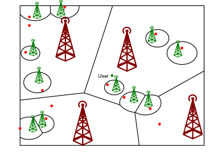
(a) Maximum downlink power association

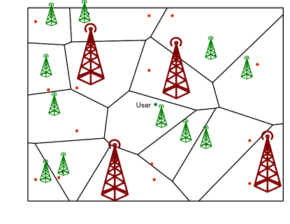
(b) Nearest AP association

Figure 1: Different association strategies and the corresponding association regions with one active UE per AP.

III Uplink $\mathtt{SINR}$ and Rate Coverage

This is the main technical section of the paper, where we detail the proposed uplink model and the corresponding analysis.

III-A General case

The uplink $\mathtt{SIR}$ CCDF of the typical UE is

$$\mathcal{P}(\tau)\triangleq{\mathbb{P}}(\mathtt{SIR}>\tau)=\sum_{k=1}^{K}{\mathbb{P}}(\mathcal{K}=k)\mathcal{P}_{k}(\tau),$$ (4)

where

$$\mathcal{P}_{k}(\tau) \triangleq{\mathbb{P}}(\mathtt{SIR}>\tau|\mathcal{K}=k)={\mathbb{P}}\left(\frac{HL{}^{\epsilon-1}}{\sum_{X\in\Phi_{u}^{b}}L_{X}^{\epsilon}H_{X}L(X,\mathcal{B})^{-1}}>\tau|\mathcal{K}=k\right)$$

$$={\mathbb{E}\left[{\exp(-L^{1-\epsilon}\tau I)|\mathcal{K}=k}\right]}={\mathbb{E}\left[{\mathcal{L}_{I|\mathcal{K}=k}(L^{1-\epsilon}\tau)}\right]},$$

where $I=\sum_{X\in\Phi_{u}^{b}}L_{X}^{\epsilon}H_{X}L(X,\mathcal{B})^{-1}$ is the uplink interference at the tagged AP $\mathcal{B}$, and $\mathcal{L}_{I|\mathcal{K}=k}$ is the Laplace transform of interference conditional on $k^{\text{th}}$ tier being the serving tier.

The following Lemma characterizes the path loss distribution of a typical UE in the given system model.

Lemma 1.

Path loss distribution at the desired link. The probability distribution function (PDF) of the path loss of a typical UE to its serving AP is

$$f_{L}(l)=\delta l^{\delta-1}\sum_{j=1}^{K}a_{j}\exp(-G_{j}l^{\delta}),\,\,l\geq 0,$$

where $\delta\triangleq\frac{2}{\alpha}$, $a_{k}={\lambda_{k}}\pi{\mathbb{E}\left[{S^{\delta}}\right]}$, $G_{k}=\sum_{j=1}^{K}a_{j}(\mathrm{T}_{j}/\mathrm{T}_{k})^{\delta}$, and the PDF, conditioned on the serving the tier being $k$, is

$$f_{L|\mathcal{K}=k}(l)\triangleq f_{L}(l|\mathcal{K}=k)=\delta G_{k}l^{\delta-1}\exp(-G_{k}l^{\delta}),\,\,l\geq 0,$$

where $\mathcal{A}_{k}\triangleq{\mathbb{P}}(\mathcal{K}=k)=\frac{a_{k}}{G_{k}}$ is the probability of the typical UE associating with tier $k$.

Proof.

The proof follows by generalizing the results in [13, 26] to our setting. Define the propagation process (introduced in [13]) from APs of tier $j$ to the typical user as $\mathcal{N}_{j}\triangleq\{L(X,0)\}_{X\in\Phi_{j}}$. The process $\mathcal{N}_{j}$ is also Poisson with intensity $\Lambda_{j}(t)=a_{j}t^{\delta},t\in\real{+}$, with $a_{j}=\pi{\lambda_{j}}{\mathbb{E}\left[{S^{\delta}}\right]}$. Therefore ${\mathbb{P}}(L_{\mathrm{min},j}>t)=\exp(-\Lambda_{j}(t))$. Path loss to the tagged AP of tier $k$ has the CCDF

$${\mathbb{P}}(L>l|\mathcal{K}=k) =\frac{{\mathbb{P}}(L_{\mathrm{min},k}>l,\mathcal{K}=k)}{{\mathbb{P}}(\mathcal{K}=k)}$$

$$=\frac{{\mathbb{P}}\left(\cap_{j=1,\neq k}^{K}L_{\mathrm{min},k}^{-1}\mathrm{T}_{k}>L_{\mathrm{min},j}^{-1}\mathrm{T}_{j}\cap L_{\mathrm{min},k}>l\right)}{\mathcal{A}_{k}}$$

$$=\frac{{\mathbb{E}_{L_{\mathrm{min},k}>l}\left[{\prod_{j=1,\neq k}^{K}\exp(-\Lambda_{j}(\hat{\mathrm{T}}_{j}L_{\mathrm{min},k}))}\right]}}{\mathcal{A}_{k}}$$

$$=\frac{\delta a_{k}}{\mathcal{A}_{k}}\int_{l}^{\infty}y^{\delta-1}\exp\left(-y^{\delta}\sum_{j=1}^{K}a_{j}\hat{\mathrm{T}}_{j}^{\delta}\right)\mathrm{d}y$$

Therefore, $f_{L}(l|\mathcal{K}=k)=\delta\frac{{a_{k}}}{\mathcal{A}_{k}}l^{\delta-1}\exp(-G_{k}l^{\delta})$ and $f_{L}(l)=\sum_{j=1}^{K}\mathcal{A}_{j}f_{L}(l|\mathcal{K}=j)$. ∎

The above distribution is not, however, identical to the distribution of the path loss between an interfering UE and its serving AP, since the latter is the conditional distribution given that the interfering UE does not associate with the tagged AP. This correlation is formalized in the corollary below.

Corollary 1.

Path loss distribution at an interfering UE. The PDF of the path loss of a UE at $X$ associated with tier $j$, conditioned on it not lying in the association cell ($\mathcal{C}_{\mathcal{B}}$) of the tagged AP at $\mathcal{B}$ of tier $k$ and the corresponding path loss $L(X,\mathcal{B})=y$, is

$$f_{L_{X}}(l|\mathcal{K}_{X}=j,\mathcal{K}=k,X\notin\mathcal{C}_{\mathcal{B}},L(X,\mathcal{B})=y)\\ =\frac{\delta G_{j}}{1-\exp(-G_{k}y^{\delta})}l^{\delta-1}\exp(-G_{j}l^{\delta}),\,\,0\leq l\leq\frac{\mathrm{T}_{j}}{\mathrm{T}_{k}}y.$$

Proof.

An interfering UE at $X$ cannot associate with the tagged AP of tier $k$ which, given the association policy, implies that the corresponding path loss is bounded as $L_{X}\leq\frac{\mathrm{T}_{j}}{\mathrm{T}_{k}}L(X,\mathcal{B})$. Noting that $G_{j}\left(\frac{\mathrm{T}_{j}}{\mathrm{T}_{k}}\right)^{\delta}=G_{k}$ results in the above distribution. ∎

Due to uplink orthogonal access within each AP, only one UE per AP transmits on the typical resource block and hence contributes to interference at the tagged AP. Therefore, $\Phi_{u}^{b}$ is not a PPP but a Poisson-Voronoi perturbed lattice (per [16]) and hence the functional form of the interference (or the Laplace functional of $\Phi_{u}^{b}$) is not tractable. Based on the following remark, we propose an approximation to characterize the corresponding process as an inhomogeneous PPP.

Remark 1.

Thinning probability. Conditioned on an AP of tier $k$ being located at $V\in\real{2}$, a UE at $U\in\real{2}$ associates with $V$ with probability ${\mathbb{P}}(\mathcal{B}_{U}=V)=\exp(-G_{k}L(V,U)^{\delta})$.

Assumption 1.

Proposed interfering UE point process. Conditioned on the tagged AP being located at $\mathcal{B}$ and of tier $k$, the propagation process of interfering UEs from tier $j$ to $\mathcal{B}$, $\mathcal{N}_{u,j}\coloneqq\{L(X,\mathcal{B})\}_{X\in\Phi_{u,j}^{b}}$ is assumed to be Poisson with intensity measure function $\Lambda_{u,j}(dx)=\delta a_{j}x^{\delta-1}(1-\exp(-G_{k}x^{\delta}))(dx)$.

The basis of the above assumption is Remark 1 along with the fact that only one UE per AP can potentially interfere with the typical UE in the uplink. Thus, the maximum density of UEs that might potentially interfere in the uplink from tier $j$ is ${\lambda_{j}}$. Assuming this parent process to be a PPP with density ${\lambda_{j}}$, the propagation process of these UEs to the tagged AP has intensity measure function $\delta a_{j}x^{\delta-1}$. However, the intensity of this parent process has to be appropriately thinned as per Remark 1 to account for the fact that these UEs do not associate with the tagged AP. The resulting process $\mathcal{N}_{u,j}$ has an intensity that increases with increasing path loss from the tagged AP.

The methodology proposed in [18] for modeling non-uniform intensity of $\Phi_{u,b}$ was based on a curve-fitting based approach and hence may not be accurate for more diverse system parameters.

Assumption 2.

Tier-wise independence. The point process of interfering UEs from each tier are assumed to be independent, i.e., the intensity measure of the interfering UEs propagation process $\mathcal{N}_{u}$ is $\Lambda_{u}(x)\triangleq\sum_{j=1}^{K}\Lambda_{u,j}(x)$.

Assumption 3.

Independent path loss. The path losses $\{L_{X}\}_{X\in\Phi_{u}^{b}}$ are assumed to follow the Gamma distribution given by Corollary 1, assumed independent (but not identically distributed).

Lemma 2.

The Laplace transform of interference at the tagged AP of tier $k$ under the proposed model is

$$\mathcal{L}_{I_{k}}(s)\triangleq\mathcal{L}_{I|\mathcal{K}=k}(s)=\exp\left(-\frac{\delta}{1-\delta}s\sum_{j=1}^{K}\hat{\mathrm{T}}_{j}^{1-\delta}a_{j}{\mathbb{E}_{L|\mathcal{K}=j}\left[{L^{\delta-(1-\epsilon)}\mathrm{C}_{\delta}\left(\frac{s\hat{\mathrm{T}}_{j}}{L^{1-\epsilon}}\right)}\right]}\right),$$ (5)

where $\mathrm{C}_{\delta}(x)\triangleq\,_{2}\mathrm{F}_{1}(1,1-\delta,2-\delta,-x)$ and ${}_{2}\mathrm{F}_{1}$ is the Gauss-Hypergeometric function.

Proof.

See Appendix A. ∎

Using the above Lemma and (4), the uplink $\mathtt{SINR}$ coverage is given in the following Theorem.

Theorem 1.

The uplink $\mathtt{SINR}$ coverage probability for the proposed uplink generative model is

$$\sum_{k=1}^{K}\delta a_{k}\int_{l>0}l^{\delta-1}\exp\left(-G_{k}l^{\delta}-\frac{\delta}{1-\delta}\tau l^{1-\epsilon}\sum_{j=1}^{K}\left(\frac{\mathrm{T}_{j}}{\mathrm{T}_{k}}\right)^{1-\delta}a_{j}{\mathbb{E}_{L|\mathcal{K}={j}}\left[{L^{\delta-(1-\epsilon)}\mathrm{C}_{\delta}\left(\frac{\tau\mathrm{T}_{j}l^{1-\epsilon}}{\mathrm{T}_{k}L^{1-\epsilon}}\right)}\right]}-\frac{\tau}{\mathtt{SNR}}l^{1-\epsilon}\right)\mathrm{d}l.$$

The $\mathtt{SIR}$ coverage can be derived by letting $\mathtt{SNR}\to\infty$ in the above theorem.

Corollary 2.

The uplink $\mathtt{SIR}$ coverage probability for the proposed uplink generative model is

$$\mathcal{P}(\tau)=\sum_{k=1}^{K}\delta a_{k}\int_{l>0}l^{\delta-1}\exp\left(-G_{k}l^{\delta}-\frac{\delta}{1-\delta}\tau l^{1-\epsilon}\sum_{j=1}^{K}\left(\frac{\mathrm{T}_{j}}{\mathrm{T}_{k}}\right)^{1-\delta}a_{j}{\mathbb{E}_{L|\mathcal{K}={j}}\left[{L^{\delta-(1-\epsilon)}\mathrm{C}_{\delta}\left(\frac{\tau\mathrm{T}_{j}l^{1-\epsilon}}{\mathrm{T}_{k}L^{1-\epsilon}}\right)}\right]}\right)\mathrm{d}l.$$

The coverage expression for the most general case involves two folds of integrals and a lookup table for the Hypergeometric function. The expression is, however, further simplified for the special cases in the next section. Useful bounds can hence be obtained in single integral-form (Corollary 3) and closed-form (Corollary 4) as below:

Corollary 3.

The uplink $\mathtt{SIR}$ coverage for the proposed generative model is upper bounded by

$$\mathcal{P}^{u}(\tau)=\sum_{k=1}^{K}\delta a_{k}\int_{l>0}l^{\delta-1}\exp\left(-G_{k}l^{\delta}-\frac{\delta\tau l^{1-\epsilon}}{(1-\delta)\Gamma(2+(1-\epsilon)/\delta)}\sum_{j=1}^{K}\left(\frac{\mathrm{T}_{j}}{\mathrm{T}_{k}}\right)^{1-\delta}a_{j}G_{j}^{(1-\epsilon)/\delta-1}\mathrm{C}_{\delta}\left(\frac{\tau\mathrm{T}_{j}l^{1-\epsilon}G_{j}^{(1-\epsilon)/\delta}}{\mathrm{T}_{k}\Gamma(2+(1-\epsilon)/\delta)}\right)\right)\mathrm{d}l.$$

Proof:

See Appendix B. ∎

Remark 2.

It can be noted from the above proof that the coverage upper bound is, in fact, exact for full channel inversion, i.e., $\epsilon=1$.

Corollary 4.

The uplink $\mathtt{SIR}$ coverage is lower bounded by

$$\mathcal{P}^{l}(\tau)=\exp\left(-\tau^{\delta}\frac{\pi^{2}\delta\epsilon(1-\epsilon)}{\sin(\pi\delta)\sin(\pi\epsilon)}\left(\sum_{k=1}^{K}\frac{{a_{k}}}{G_{k}^{2-\epsilon}}\right)\left(\sum_{k=1}^{K}\frac{{a_{k}}}{G_{k}^{\epsilon}}\right)\right).$$

Proof.

See Appendix C. ∎

III-B Special cases

For the following plausible special cases, the uplink $\mathtt{SIR}$ coverage expression is further simplified.

Corollary 5.

($K=1$) The uplink $\mathtt{SIR}$ coverage in a single tier network with density ${\lambda_{1}}$ is

$$\mathcal{P}(\tau)=\delta{a_{1}}\int_{l>0}l^{\delta-1}\exp\left(-{a_{1}}l^{\delta}-\frac{\delta}{1-\delta}\tau l^{1-\epsilon}{a_{1}}{\mathbb{E}_{L}\left[{L^{\delta-(1-\epsilon)}\mathrm{C}_{\delta}\left(\frac{\tau l^{1-\epsilon}}{L^{1-\epsilon}}\right)}\right]}\right)\mathrm{d}l,$$

where ${a_{1}}={\lambda_{1}}\pi{\mathbb{E}\left[{S^{\delta}}\right]}$.

The above expression differs from the one in [10] due to the proposed interference characterization. In [10], the distribution of path loss of each interfering UE to its serving AP was assumed i.i.d.

Corollary 6.

($\mathrm{T}_{j}=\mathrm{T}_{k}\forall j,k$) The uplink $\mathtt{SIR}$ coverage in a $K$-tier network with min-path loss association is the same as the coverage of a single tier network with density ${\lambda}=\sum_{k=1}^{K}{\lambda_{k}}$.

Corollary 7.

($\epsilon=0$) Without uplink power control, the uplink $\mathtt{SIR}$ coverage is

$$\mathcal{P}(\tau)=\sum_{k=1}^{K}\delta a_{k}\int_{l>0}l^{\delta-1}\exp\left(-G_{k}l^{\delta}-{a}\int_{0}^{\infty}\frac{1-\exp(-G_{k}x)}{1+(\tau l)^{-1}x^{-1/\delta}}\mathrm{d}x\right)\mathrm{d}l,$$

where $a=\sum_{j=1}^{K}a_{j}$.

Corollary 8.

($\epsilon=1$) With full channel inversion, the coverage is

$$\mathcal{P}(\tau)=\sum_{k=1}^{K}\frac{{a_{k}}}{G_{k}}\exp\left(-\frac{\delta}{\delta-1}\tau\sum_{j=1}^{K}\left(\frac{\mathrm{T}_{j}}{\mathrm{T}_{k}}\right)^{1-\delta}\frac{{a_{j}}}{G_{j}}\mathrm{C}_{\delta}\left(\tau\frac{\mathrm{T}_{j}}{\mathrm{T}_{k}}\right)\right).$$

Corollary 9.

($\epsilon=0,\mathrm{T}_{j}=\mathrm{T}_{k}\forall j,k$) Without power control and with min path loss association, the uplink $\mathtt{SIR}$ coverage is

$$\mathcal{P}(\tau)=\delta{a}\int_{l>0}l^{\delta-1}\exp\left(-{a}l^{\delta}-{a}\frac{\delta}{1-\delta}\tau l{\mathbb{E}_{L}\left[{L^{\delta-1}\mathrm{C}_{\delta}\left(\frac{\tau l}{L}\right)}\right]}\right)\mathrm{d}l.$$

Corollary 10.

($\epsilon=1,\mathrm{T}_{j}=\mathrm{T}_{k}\forall j,k$) With full channel inversion based power control and with min path loss association, the uplink $\mathtt{SIR}$ coverage is

$$\mathcal{P}(\tau)=\exp\left(-\frac{\delta\tau}{1-\delta}\mathrm{C}_{\delta}(\tau)\right).$$

Remark 3.

Comparison with downlink. The downlink $\mathtt{SIR}$ coverage derived in [23] for max downlink received power association, when adapted to the current setting, is $\frac{1}{1+\frac{\delta\tau}{1-\delta}\mathrm{C}_{\delta}(\tau)}$. Since ${1+x}<\exp(x),\,\,\forall x>0$, downlink $\mathtt{SIR}$ stochastically dominates the uplink $\mathtt{SIR}$ of Corollary 10.

Remark 4.

Density invariance. Corollary 10 highlights the independence of uplink $\mathtt{SIR}$ coverage on infrastructure density in HCNs with minimum path loss association and full channel inversion. This trend is similar to the result proved for downlink $\mathtt{SIR}$ in macrocellular networks [12] and HCNs [24, 23].

III-C Uplink rate distribution

The rate of a user depends on both the $\mathtt{SINR}$ and load at the tagged AP (as per (3)), which in turn depends on the corresponding association area $|\mathcal{C}_{\mathcal{B}}|$. The weighted path loss association and PPP placement of APs leads to complex association cells (see Fig. 1) whose area distribution is not known. However, the association policy is stationary [25] and hence the mean uplink association area of a typical AP of tier $k$ is $\frac{\mathcal{A}_{k}}{{\lambda_{k}}}$. The association area approximation proposed in [15] is used to quantify the uplink load distribution at the tagged AP as

$$\mathsf{K}_{t}(\lambda_{u}\mathcal{A}_{k},{\lambda_{k}},n)\triangleq{\mathbb{P}}(N=n|\mathcal{K}=k)=\frac{3.5^{3.5}}{(n-1)!}\frac{\Gamma(n+3.5)}{\Gamma(3.5)}\left(\frac{\lambda_{u}\mathcal{A}_{k}}{{\lambda_{k}}}\right)^{n-1}\left(3.5+\frac{\lambda_{u}\mathcal{A}_{k}}{{\lambda_{k}}}\right)^{-(n+3.5)}\,\,,n\geq 1.$$

Using Corollary 2 and (3), and assuming the independence between $\mathtt{SINR}$ and load, the uplink rate coverage is given in the following Theorem.

Theorem 2.

Under the presented system model and assumptions, the uplink rate coverage is given by

$$\mathcal{R}(\rho)=\sum_{k=1}^{K}\mathcal{A}_{k}\sum_{n>0}\mathsf{K}_{t}(\lambda_{u}\mathcal{A}_{k},{\lambda_{k}},n)\mathcal{P}_{k}(2^{\hat{\rho}n}-1),$$

where $\mathcal{P}_{k}$ is given in Corollary 2 and $\hat{\rho}\triangleq\rho(\eta\mathrm{W})^{-1}$.

Proof.

Using the rate expression in (3)

$${\mathbb{P}}(\mathtt{Rate}>\rho) ={\mathbb{P}}(\mathtt{SINR}>2^{\hat{\rho}{N}}-1)=\sum_{k=1}^{K}\mathcal{A}_{k}{\mathbb{P}}(\mathtt{SINR}>2^{\hat{\rho}{N}}-1|\mathcal{K}=k)$$

$$=\sum_{k=1}^{K}\mathcal{A}_{k}\sum_{n>0}\mathsf{K}_{t}(\lambda_{u}\mathcal{A}_{k},{\lambda_{k}},n){\mathbb{P}}\left(\mathtt{SINR}>2^{\hat{\rho}n}-1|\mathcal{K}=k,{N}=n\right),$$

where $\hat{\rho}=\rho(\eta\mathrm{W})^{-1}$ is the normalized rate threshold. Since APs with larger association regions have higher load and larger user to AP distance, therefore the load and $\mathtt{SINR}$ are correlated. For tractability, this dependence and thermal noise are ignored, as in [15], to yield

$${\mathbb{P}}\left(\mathtt{SINR}>2^{\hat{\rho}n}-1|\mathcal{K}=k,{N}=n\right)\approx\mathcal{P}_{k}(2^{\hat{\rho}n}-1).$$

∎

Corollary 11.

If the load at each AP is approximated by its respective mean, $\bar{N}_{k}\triangleq{\mathbb{E}\left[{N|\mathcal{K}=k}\right]}=1+1.28\frac{\mathcal{A}_{k}{\lambda_{u}}}{{\lambda_{k}}}$ [15], the uplink rate coverage is

$$\bar{\mathcal{R}}(\rho)=\sum_{k=1}^{K}\mathcal{A}_{k}\mathcal{P}_{k}(2^{\hat{\rho}\bar{N}_{k}}-1).$$

The corollary above simplifies the rate coverage expression of Theorem 2 by eliminating a sum and sacrificing a bit of accuracy.

IV Joint uplink-downlink rate coverage

The joint uplink-downlink rate coverage is defined formally below.

Definition 1.

The uplink-downlink joint rate coverage is the probability that the rate on both links exceed their respective thresholds, i.e.,

$$\mathcal{R}^{J}(\rho_{u},\rho_{d}) \triangleq{\mathbb{P}}(\text{Uplink rate }>\rho_{u},\text{ Downlink rate }>\rho_{d}).$$

It can be equivalently interpreted as the fraction of users in the network whose both uplink and downlink rate exceed their respective thresholds.

For deriving the joint coverage, the joint path loss distribution needs to be characterized. For the special case of coupled association, the path losses are identical, however, for the general case they are correlated. The following Lemma characterizes the joint distribution of path losses for arbitrary downlink and uplink association weights.

Lemma 3.

Joint path loss distribution. The joint PDF of uplink path loss ($L$) and downlink path loss ($L^{{}^{\prime}}$) for the typical user under the given setting is

$$f_{L,L^{{}^{\prime}}}(x,y,\mathcal{K}=k,\mathcal{K}^{{}^{\prime}}=j)\\ =\begin{cases}{a_{j}}{a_{k}}\delta^{2}x^{\delta-1}y^{\delta-1}\exp\left(-\sum_{i=1}^{K}{a_{i}}\max\left(\frac{\mathrm{T}_{i}^{{}^{\prime}}}{\mathrm{T}_{j}^{{}^{\prime}}}y,\frac{\mathrm{T}_{i}}{\mathrm{T}_{k}}x\right)^{\delta}\right),&k\neq j,\,\,\frac{\mathrm{T}_{j}}{\mathrm{T}_{k}}\leq\frac{\mathrm{T}_{j}^{{}^{\prime}}}{\mathrm{T}_{k}^{{}^{\prime}}},\,\,\,x\geq 0,\,\,\frac{\mathrm{T}_{j}}{\mathrm{T}_{k}}\leq\frac{y}{x}\leq\frac{\mathrm{T}_{j}^{{}^{\prime}}}{\mathrm{T}_{k}^{{}^{\prime}}}\\ {a_{k}}\delta x^{\delta-1}\exp\left(-x^{\delta}\sum_{i=1}^{K}{a_{i}}\max\left(\frac{\mathrm{T}_{i}^{{}^{\prime}}}{\mathrm{T}_{k}^{{}^{\prime}}},\frac{\mathrm{T}_{i}}{\mathrm{T}_{k}}\right)^{\delta}\right),&k=j,\,\,x\geq 0,\,\,y=x\\ 0&\text{ otherwise.}\end{cases}\normalsize$$

Proof.

For $\mathcal{K}=\mathcal{K}^{{}^{\prime}}=k$,

$${\mathbb{P}}(L=L^{{}^{\prime}}>x,\mathcal{K}=\mathcal{K}^{{}^{\prime}}=k) ={\mathbb{P}}\left(\bigcap_{i=1,\neq k}^{K}L_{\mathrm{min},i}>L_{\mathrm{min},k}\max\left(\frac{\mathrm{T}_{i}^{{}^{\prime}}}{\mathrm{T}_{k}^{{}^{\prime}}},\frac{\mathrm{T}_{i}}{\mathrm{T}_{k}}\right)\bigcap L_{\mathrm{min},k}>x\right)$$

$$=\delta{a_{k}}\int_{x}^{\infty}l^{\delta-1}\exp\left(-l^{\delta}\sum_{i=1}^{K}{a_{i}}\max\left(\frac{\mathrm{T}_{i}^{{}^{\prime}}}{\mathrm{T}_{k}^{{}^{\prime}}},\frac{\mathrm{T}_{i}}{\mathrm{T}_{k}}\right)^{\delta}\right)\mathrm{d}l.$$

And for $\mathcal{K}=k,\mathcal{K}^{{}^{\prime}}=j$ with $k\neq j$ and $\frac{\mathrm{T}_{j}^{{}^{\prime}}}{\mathrm{T}_{k}^{{}^{\prime}}}>\frac{\mathrm{T}_{j}}{\mathrm{T}_{k}}$

$${\mathbb{P}}(L>x,L^{{}^{\prime}}>y,\mathcal{K}=k,\mathcal{K}^{{}^{\prime}}=j)\\ ={\mathbb{P}}\left(\bigcap_{i=1,\neq k,j}^{K}L_{\mathrm{min},i}>\max\left(\frac{\mathrm{T}_{i}^{{}^{\prime}}}{\mathrm{T}_{j}^{{}^{\prime}}}L_{\mathrm{min},j},\frac{\mathrm{T}_{i}}{\mathrm{T}_{k}}L_{\mathrm{min},k}\right)\bigcap\left\{\frac{\mathrm{T}_{j}}{\mathrm{T}_{k}}L_{\mathrm{min},k}\leq L_{\mathrm{min},j}\leq\frac{\mathrm{T}_{j}^{{}^{\prime}}}{\mathrm{T}_{k}^{{}^{\prime}}}L_{\mathrm{min},k}\right\}\bigcap\{L_{\mathrm{min},k}>x\},\bigcap\{L_{\mathrm{min},j}>y\}\right)\\ =\delta^{2}{a_{j}}{a_{k}}\int_{x}^{\infty}\int_{\max(\mathrm{T}_{j}/\mathrm{T}_{k}t,y)}^{\mathrm{T}_{j}^{{}^{\prime}}/\mathrm{T}_{k}^{{}^{\prime}}t}t^{\delta-1}u^{\delta-1}\exp\left(-\sum_{i=1}^{K}{a_{i}}\max\left(\frac{\mathrm{T}_{i}^{{}^{\prime}}}{\mathrm{T}_{j}^{{}^{\prime}}}t,\frac{\mathrm{T}_{i}}{\mathrm{T}_{k}}u\right)^{\delta}\right)\mathrm{d}u\mathrm{d}t$$

Differentiating the above CCDFs leads to the corresponding PDFs. ∎

The downlink $\mathtt{SIR}$ analysis in [23] ignored shadowing. However the analysis can be adapted to the presented setting to give the Laplace transform of the downlink interference in the following Lemma (presented without proof).

Lemma 4.

The Laplace transform of downlink interference ($I^{{}^{\prime}}$) when the serving (downlink) AP belongs to tier $j$ and the corresponding path loss is $l$, i.e. $L^{{}^{\prime}}=l$, is

$$\mathcal{L}_{I^{{}^{\prime}}_{j}}(s|L^{{}^{\prime}}=l)=\exp\left\{-\frac{\delta}{1-\delta}sl^{\delta-1}\sum_{i=1}^{K}{a_{i}}\mathrm{P}_{i}\hat{\mathrm{T}}_{i}^{{}^{\prime}(\delta-1)}\mathrm{C}_{\delta}(s\mathrm{P}_{i}/l\hat{\mathrm{T}}_{i}^{{}^{\prime}})\right\}.$$

Theorem 3.

Using the mean load approximation for uplink and downlink, and assuming the uplink and downlink interference to be independent, the joint uplink-downlink rate coverage is

$$\mathcal{R}^{J}(\rho_{u},\rho_{d})=\sum_{k=1}^{K}\sum_{j=1}^{J}\int_{0}^{\infty}\int_{0}^{\infty}\mathcal{L}_{I_{k}}\left(x^{1-\epsilon}v(\hat{\rho}_{u}\bar{N}_{k})\right)\mathcal{L}_{I^{\prime}_{j}}\left(y\mathrm{P}_{j}v(\hat{\rho}_{d}\bar{N}_{k}^{{}^{\prime}})\right)f_{L,L^{{}^{\prime}}}(x,y,\mathcal{K}=k,\mathcal{K}^{{}^{\prime}}=j)\mathrm{d}x\mathrm{d}y,$$

where $\bar{N}_{k}=1+1.28\frac{{\lambda_{u}}}{{\lambda_{k}}}\frac{{a_{k}}}{\sum_{j=1}^{K}a_{j}\hat{\mathrm{T}}_{j}^{\delta}}$ is the average uplink load at the AP serving in the uplink, $\bar{N}_{k}^{{}^{\prime}}=1+1.28\frac{{\lambda_{u}}}{{\lambda_{k}}}\frac{{a_{k}}}{\sum_{j=1}^{K}a_{j}\hat{\mathrm{T}}_{j}^{{{}^{\prime}}\delta}}$ is the average downlink load at the AP serving in the downlink, $\hat{\rho}_{u}=\rho(\mathrm{W}\eta)^{-1}$, $\hat{\rho}_{d}=\rho(\mathrm{W}(1-\eta))^{-1}$, and $\mathcal{L}_{I_{k}},\mathcal{L}_{I^{\prime}_{j}}$ are as defined in Lemma 2 and 4 respectively.

Proof.

The proof follows by noting that the joint rate coverage can be written in terms of joint $\mathtt{SIR}$ coverage as in Theorem 2. Assuming independence of uplink and downlink interference, the joint $\mathtt{SIR}$ coverage is

$${\mathbb{P}}(\text{ Uplink }\mathtt{SIR}>\tau_{u},\text{Downlink }\mathtt{SIR}>\tau_{d})=\sum_{k=1}^{K}\sum_{j=1}^{J}{\mathbb{E}\left[{\mathbbm{1}(\mathcal{K}=k)\mathbbm{1}(\mathcal{K}^{{}^{\prime}}=j)\mathcal{L}_{I_{k}}\left(L^{1-\epsilon}\tau_{u}\right)\mathcal{L}_{I^{\prime}_{j}}\left(L^{{}^{\prime}}\mathrm{P}_{j}\tau_{d}\right)}\right]}.$$

The final expression is then obtained by using the rate model of (3) along with Lemma 3. ∎

V Validation through simulations

The proposed model and the corresponding analytical results are validated by simulations (based on the model of Sec. II) in a two tier setting with ${\lambda_{1}}=5$ BS per sq. km, $\alpha=3.5$, $S$ assumed Lognormal with $8$ dB standard deviation, open loop power spectral density $\mathrm{P}_{u}=-80$ dBm/Hz, and free space path loss $\mathrm{L_{0}}=-40$ dB is assumed at reference distance of $1$ m at carrier frequency of $2$ GHz (the same parameters are used in the later sections unless otherwise specified). Fig. 2 shows the uplink $\mathtt{SINR}$ distribution obtained from simulations along with the $\mathtt{SIR}$ distribution from analysis (Corollary 2) for different association weights and tier 2 densities. Two simplifications of the analysis A1, A2 are also shown for the $\epsilon=1$ case. A1 neglects the conditioning of the transmit power of an interfering user, i.e. Lemma 1 is used for path loss distribution of interfering UEs instead of Corollary 1. A2 additionally neglects the proposed modeling of interfering UE process as per Assumption 1 and instead models interfering UEs of each tier as an homogeneous PPP with density same as the corresponding tier density. The plots lead to the following takeaways: 1. the proposed analysis matches the simulations quite closely for a range of parameters, validating Assumptions 1, 2, and 3; 2. neglecting the proposed thinning and/or conditioning (as is done prior works) leads to significant diversion from actual coverage, and 3. thermal noise has a minimal impact on uplink $\mathtt{SINR}$ (this could also be due to the higher BS density). Note that a value of $\hat{\mathrm{T}}_{2}=-20$ dB corresponds to a typical power difference between small cells and macrocells and hence is equivalent to downlink maximum power association.

The rate coverage obtained from simulation and analysis (Corollary 11) is compared for a two-tier setting in Fig. 3a and for a three-tier setting in Fig. 3b. The user density used in these plots is ${\lambda_{u}}=200$ per sq. km. The joint rate distribution derived from analysis and simulation is shown in Fig. 4 for an uplink resource fraction $\eta=0.5$. The close match between analysis and simulations for a wide range of parameters in these plots validates the mean load assumption and the downlink-uplink interference independence assumption.

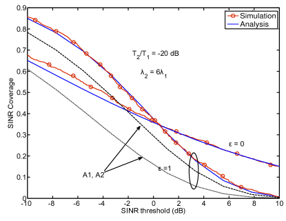
(a) ${\lambda_{2}}=6{\lambda_{1}}$, $\mathrm{T}_{2}/\mathrm{T}_{1}=-20$ dB

(b) ${\lambda_{2}}=4{\lambda_{1}}$, $\mathrm{T}_{2}/\mathrm{T}_{1}=0$ dB

Figure 2: Comparison of uplink $\mathtt{SINR}$ distribution from simulation with $\mathtt{SIR}$ distribution from analysis.

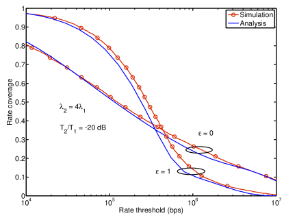
(a) ${\lambda_{2}}=6{\lambda_{1}}$, $\mathrm{T}_{2}/\mathrm{T}_{1}=-20$ dB

(b) ${\lambda_{3}}=7{\lambda_{1}}$, ${\lambda_{2}}=4{\lambda_{1}}$, $\mathrm{T}_{3}=\mathrm{T}_{2}=\mathrm{T}_{1}$

Figure 3: Comparison of uplink rate distribution from analysis and simulation.

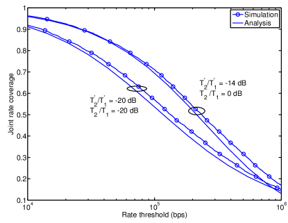
Figure 4: Comparison of joint rate coverage from analysis and simulation (with ${\lambda_{2}}=6{\lambda_{1}}$ and $\epsilon=0.5$).

VI Optimal power control and association

The uplink $\mathtt{SIR}$ and rate coverage probability expressions of Corollary 2, Theorem 2, and 3 can be used to numerically find the optimal power control and association weights. However, first we focus on the coverage lower bound $\mathcal{P}^{l}$ of Corollary 4 and obtain the following proposition.

Proposition 1.

Minimum path loss association maximizes $\mathcal{P}^{l}$ $\forall\epsilon\in[0,1]\,\,\forall\tau$. Further, $\epsilon=0.5$ maximizes the coverage lower bound $\mathcal{P}^{l}$.

Proof.

Using Corollary 4, $\mathcal{P}^{l}$ is maximized with $\{\mathrm{T}_{j}^{*}\}$ given by

$$\{\mathrm{T}_{j}^{*}\}_{j=1}^{K} =\operatorname*{arg\,min}\sum_{k=1}^{K}\frac{{a_{k}}}{G_{k}^{2-\epsilon}}\sum_{k=1}^{K}\frac{{a_{k}}}{G_{k}^{\epsilon}}=\operatorname*{arg\,min}\frac{(\sum_{k=1}^{K}{a_{k}}\mathrm{T}_{k}^{2-\epsilon})(\sum_{k=1}^{K}{a_{k}}\mathrm{T}_{k}^{\epsilon})}{(\sum_{j=1}^{K}{a_{j}}\mathrm{T}_{j})^{2}}$$

$$=1+\operatorname*{arg\,min}\frac{\sum_{i\neq j}{a_{i}}{a_{j}}(\mathrm{T}_{i}^{2-\epsilon}\mathrm{T}_{j}^{\epsilon}-\mathrm{T}_{i}\mathrm{T}_{j})}{(\sum_{j=1}^{K}{a_{j}}\mathrm{T}_{j})^{2}},$$

where the last equation is minimized with $\mathrm{T}_{j}=\mathrm{T}_{k}$ $\forall j,k$. Moreover, for such a case

$$\mathcal{P}^{l}(\tau)=\exp\left(-\tau^{\delta}\frac{\pi^{2}\delta\epsilon}{\sin(\pi\delta)\sin(\pi\epsilon)}\right),$$

which is maximized for $\epsilon=0.5$. ∎

Remark 5.

Since the lower bound overestimates the uplink interference by neglecting the correlation of the transmit power of an interfering user with its path loss to the tagged AP (and hence treating it as if originating from an ad-hoc network), the result of optimal PCF of $0.5$ is in agreement with results for ad hoc wireless networks [27, 28] (derived under quite different modeling assumptions, though).

Power control. Since the power control impacts only uplink $\mathtt{SIR}$ and not load (unlike association), the optimal PCF is obtained using the $\mathtt{SIR}$ coverage of Corollary 2. The $\mathtt{SIR}$ threshold plays a vital role in determining the optimal PCF. More channel inversion is more beneficial for cell edge UEs, as they suffer from higher path loss and as a result the optimal PCF decreases with $\mathtt{SIR}$ threshold, as shown in Fig. 5. This is similar to the insight obtained for single-tier networks in [10]. It is interesting to note that the result on optimal PCF of Proposition 1 applies only to moderate $\mathtt{SIR}$ thresholds. Further, as can be observed a higher association weight imbalance leads to a uniform (across all thresholds) increase in the optimal PCF, as the path losses in the network increase. It can also be observed that the optimal PCF is relatively insensitive to different densities in the two tier network, with no dependence seen in the case of minimum path loss association. A similar trend translates to uplink rate distribution too. The variation of uplink fifth percentile rate (or edge rate, $\rho|\mathcal{R}(\rho)=0.95$) and median rate ($\rho|\mathcal{R}(\rho)=0.50$) with PCF is shown in Fig. 6. A higher PCF maximizes fifth percentile rate than that for median rate, since former represents users with lower uplink $\mathtt{SIR}$.

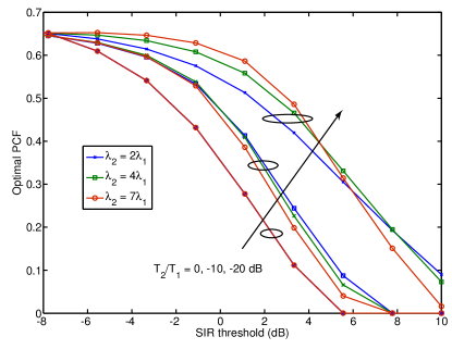
Figure 5: Variation of the optimal PCF with $\mathtt{SIR}$ threshold (obtained from Corollary 2) for various association weights and densities. The bottom ($0$ dB) curve is indistinguishable for all ${\lambda_{2}}$.

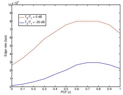
(a)

(b)

Figure 6: Variation of uplink edge and median rate with PCF (obtained from Corollary 11) for ${\lambda_{2}}=6{\lambda_{1}}$ per sq. km.

Figure 7: Uplink $\mathtt{SIR}$ variation with association weights (obtained from Corollary 2) with ${\lambda_{2}}=5{\lambda_{1}}$ for different thresholds and PCFs.

Uplink association weights. The variation of uplink $\mathtt{SIR}$ coverage with association weights is shown in Fig. 7 for different PCFs and $\mathtt{SIR}$ thresholds. Association weights are seen to affect the $\mathtt{SIR}$ coverage nominally, except for the no power control case (where the variation is in concurrence with the result of the Proposition 1). An intuitive explanation of this behavior is as follows: higher weight imbalance may lead a user to associate with a farther macrocell with a higher path loss, but it would also experience reduced uplink interference due to the larger association area of the corresponding AP. So these two contrary effects compensate for each other leading to the observed phenomenon.

It is worth noting here that minimum path loss association leads to identical load distribution across all APs and hence balances the load. Moreover due to no adverse effect on uplink $\mathtt{SIR}$, minimum path loss association is also seen to be optimal from rate perspective too. The trend of uplink edge (fifth percentile) and median rate with association weights is shown in Fig. 8. As can be seen, irrespective of the PCF and density, minimum path loss association is optimal for uplink rate. Note that these results and insights for uplink are in contrast with the corresponding result for downlink, where maximum $\mathtt{SIR}$ association (equivalent to maximum downlink received power association) is optimal for downlink $\mathtt{SIR}$ coverage [23], and hence a conservative association bias was shown to be optimal for rate coverage [22, 29].

(a) Edge rate, $\epsilon=1$

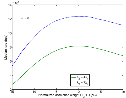
(b) Median rate, $\epsilon=0$

Figure 8: Variation of uplink edge and median rate with association weights (obtained from Corollary 11).

Uplink-downlink jointly optimal association. Considered separately, as discussed in the previous section, the association weights $\frac{\mathrm{T}_{2}}{\mathrm{T}_{1}}=0$ dB, $\frac{\mathrm{T}_{2}^{{}^{\prime}}}{\mathrm{T}_{1}^{{}^{\prime}}}=-14$ dB optimize the uplink and downlink rate respectively. However, what happens if the joint downlink and uplink association is considered? The variation of joint rate coverage as a function of downlink and uplink association weights is shown in Fig. 9 for three pairs of ($\epsilon,\eta$) with a rate threshold of $\rho_{u}=\rho_{d}=128$ Kbps and ${\lambda_{2}}=6{\lambda_{1}}$. As can be seen from the plots, the uplink and downlink association weights of $\frac{\mathrm{T}_{2}}{\mathrm{T}_{1}}=0$ dB, $\frac{\mathrm{T}_{2}^{{}^{\prime}}}{\mathrm{T}_{1}^{{}^{\prime}}}=-14$ dB ($\mathrm{T}_{1}=\mathrm{T}_{1}^{{}^{\prime}}=1$ in these plots) also maximize the joint uplink-downlink rate coverage irrespective of chosen $\eta$ and $\epsilon$. These leads to two key observations: (i) the uplink and downlink association weights that maximize the joint rate coverage are the same as the ones that maximize their individual link coverage, and as a result (ii) decoupled association, i.e. different association weights for the uplink and downlink, is optimal for joint coverage.

(a) $\epsilon=0$, $\eta=0.7$

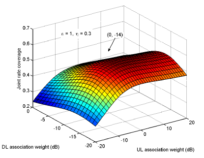
(b) $\epsilon=1$, $\eta=0.3$

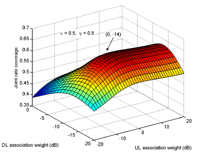
(c) $\epsilon=0.5$, $\eta=0.5$

Figure 9: Variation of joint rate coverage with uplink and downlink association weights (obtained from Theorem 3) for different ($\epsilon$, $\eta$) pairs.

Optimal coupled vs. decoupled association. In Fig. 10, the gains of optimal decoupled association over that of coupled are analytically assessed for edge rate and median rates for varying PCFs with ${\lambda_{2}}=6{\lambda_{1}}$ and $\eta=0.5$. Note that in these plots, the rates corresponds the minimum of uplink and downlink, i.e. edge rate $=\rho|\mathcal{R}^{J}(\rho,\rho)=0.95$ and median rate $=\rho|\mathcal{R}^{J}(\rho,\rho)=0.5$. As observed, across all PCFs, the decoupled association provides significant ($\sim 1.5$x) gain over coupled association. This shows that, in spite requiring certain architectural changes [20], decoupled association is beneficial for applications requiring similar QoS in both uplink and downlink.

(a) Joint edge rate

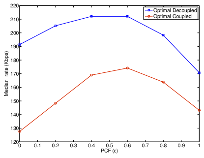
(b) Joint median rate

Figure 10: Variation of uplink-downlink joint edge and median rate with PCF (obtained from Theorem 3) for optimal coupled and decoupled association.

VII Conclusion

This paper proposes a novel model to analyze uplink $\mathtt{SINR}$ and rate coverage in $K$-tier HCNs with load balancing. To the best of the authors’ knowledge, this is the first work to derive and validate the uplink rate distribution in HCNs incorporating offloading and fractional power control. One of the key takeaways from this work is the contrasting behavior exhibited by the uplink and downlink rate distributions with respect to load balancing. The derivation of uplink $\mathtt{SINR}$ and rate distribution as a tractable functional form of system parameters opens various areas to gain further design insights. For example, optimal association weights were derived in this paper for both uplink and joint uplink-downlink coverage. We assumed parametric but fixed resource partitioning between uplink and downlink – and this might also be a more practical assumption – but analyzing the impact of more dynamic (possibly load-aware) partitioning on the presented insights could be considered in the future. The proposed uplink interference characterization can also be used to analyze systems like massive MIMO, where it plays a crucial role [30]. Performance analysis for decoupled association incorporating the cost of possible architectural changes [20] could also be one area of future investigation.

Appendix A

Derivation of Lemma 2.

Let $\mathcal{L}_{I_{kj}}(s)$ denote the Laplace transform of the interference from tier $j$ UEs, then $\mathcal{L}_{I_{k}}=\prod_{j=1}^{K}\mathcal{L}_{I_{kj}}$ (from Assumption 2). Now,

$$\mathcal{L}_{I_{kj}}(s) ={\mathbb{E}\left[{\exp\left(-s\sum_{X\in\Phi_{u,j}^{b}}L_{X}^{\epsilon}H_{X}L(X,\mathcal{B})^{-1}\right)}\right]}$$

$$\overset{(a)}{=} {\mathbb{E}\left[{\prod_{X\in\Phi_{u,j}^{b}}\frac{1}{1+sL_{X}^{\epsilon}L(X,\mathcal{B})^{-1}}}\right]}$$

$$= {\mathbb{E}\left[{\prod_{X\in\mathcal{N}_{u,j}}{\mathbb{E}_{L_{X}}\left[{\frac{1}{1+sL_{X}^{\epsilon}X^{-1}}}\right]}}\right]}$$

$$\overset{(b)}{=} \exp\left(-\int_{x>0}\left(1-{\mathbb{E}_{L_{x}}\left[{\frac{1}{1+sL_{x}^{\epsilon}x^{-1}}}\right]}\right)\Lambda_{u,j}(\mathrm{d}x)\right)$$

$$\overset{(c)}{=} \exp\left(-\int_{x>0}\left(1-{\mathbb{E}_{L}\left[{\frac{1}{1+sL^{\epsilon}x^{-1}}\mid L<\hat{\mathrm{T}}_{j}x,\mathcal{K}_{x}=j}\right]}\right)\Lambda_{u,j}(\mathrm{d}x)\right)$$

$$= \exp\left(-\int_{x>0}{\mathbb{E}_{L}\left[{\frac{1}{1+(sL^{\epsilon})^{-1}x}\mid L<\hat{\mathrm{T}}_{j}x,\mathcal{K}_{x}=j}\right]}\Lambda_{u,j}(\mathrm{d}x)\right)$$

$$= \exp\left(-{\mathbb{E}_{L|\mathcal{K}=j}\left[{a_{j}L^{\delta}\hat{\mathrm{T}}_{j}^{-\delta}\int_{1}^{\infty}\frac{\mathrm{d}t}{1+(s\hat{\mathrm{T}}_{j})^{-1}L^{1-\epsilon}t^{1/\delta}}}\right]}\right),$$

where (a) follows from the i.i.d. nature of $\{H_{X}\}$, (b) follows from the Laplace functional (also known as probability generating functional) of the assumed PPP $\mathcal{N}_{u,j}$, (c) follows from Corollary 1, and the last equality follows with change of variables $t=(x\hat{\mathrm{T}}_{j}/L)^{\delta}$ and algebraic manipulation. The final result is then obtained by using the definition of Gauss-Hypergeometric function, yielding

$$\int_{1}^{\infty}\frac{\mathrm{d}t}{1+t^{1/\delta}L^{1-\epsilon}(s\hat{\mathrm{T}}_{j})^{-1}}\\ =\frac{\delta}{1-\delta}\frac{s\hat{\mathrm{T}}_{j}}{L^{1-\epsilon}}\,_{2}\mathrm{F}_{1}\left(1,1-\delta,2-\delta,-\frac{s\hat{\mathrm{T}}_{j}}{L^{1-\epsilon}}\right).$$

∎

Appendix B •

Derivation of Corollary 3.

The proof of Lemma 2 gives

$$\mathcal{L}_{I_{kj}}(s) =\exp\left(-a_{j}\hat{\mathrm{T}}_{j}^{-\delta}\int_{l>0}l^{\delta}\int_{1}^{\infty}\frac{\mathrm{d}t}{1+(s\hat{\mathrm{T}}_{j})^{-1}l^{1-\epsilon}t^{1/\delta}}f_{L|\mathcal{K}=j}(l)\mathrm{d}l\right)$$

$$=\exp\left(-\frac{a_{j}\hat{\mathrm{T}}_{j}^{-\delta}}{G_{j}}\int_{1}^{\infty}\int_{l>0}\frac{1}{1+(s\hat{\mathrm{T}}_{j})^{-1}l^{1-\epsilon}t^{1/\delta}}f_{L^{\prime}|\mathcal{K}=j}(l)\mathrm{d}l\mathrm{d}t\right),$$

where the inner integral (w.r.t $l$) can be viewed as an expectation of $1/(1+t^{1/\delta}L^{\prime 1-\epsilon}(s\hat{\mathrm{T}}_{j})^{-1})$, where $L_{j}^{\prime}$ is a random variable with pdf $f_{L^{\prime}|\mathcal{K}=j}(l)=\delta G_{j}^{2}l^{2\delta-1}\exp(-G_{j}l^{\delta})$ for $l>0$. Since $1/(1+t^{1/\delta}x(s\hat{\mathrm{T}}_{j})^{-1})$ is a convex function of $x$, we can apply Jensen’s inequality (using ${\mathbb{E}\left[{L^{{}^{\prime}(1-\epsilon)}|\mathcal{K}=j}\right]}=\frac{\Gamma(2+(1-\epsilon)/\delta)}{G_{j}^{(1-\epsilon)/\delta}}$) and obtain a lower bound on the inner integral, which leads to an upper bound on the coverage probability in a form similar to the one in Corollary 2. ∎

Appendix C •

Derivation of Corollary 4.

Neglecting the conditioning in (c) of the proof of Lemma 2, we have

$$\mathcal{L}_{I_{k}}(s)\geq\exp\left(-\sum_{j=1}^{K}\int_{x>0}{\mathbb{E}_{L|\mathcal{K}=j}\left[{\frac{1}{1+(sL^{\epsilon})^{-1}x}}\right]}\Lambda_{u,j}(\mathrm{d}x)\right)$$

$$\geq\exp\left(-\sum_{j=1}^{K}{\mathbb{E}_{L|\mathcal{K}=j}\left[{\int_{x>0}\frac{1}{1+(sL^{\epsilon})^{-1}x}\delta{a_{j}}x^{\delta-1}\mathrm{d}x}\right]}\right)$$

$$\overset{(a)}{=}\exp\left(-s^{\delta}\frac{\pi\delta}{\sin(\pi\delta)}\sum_{j=1}^{K}{a_{j}}{\mathbb{E}_{L|\mathcal{K}=j}\left[{L^{\delta\epsilon}}\right]}\right),$$

where (a) follows by the change of variables $t=x^{\delta}(sL^{\epsilon})^{-2/\alpha}$ and noting that $\int_{0}^{\infty}\frac{\mathrm{d}t}{1+t^{\alpha/2}}=\frac{2\pi}{\alpha\sin(2\pi/\alpha)}$. Now using the coverage expression

$$\mathcal{P}(\tau) \geq{\mathbb{E}\left[{\exp\left(-\frac{\pi\delta}{\sin(\pi\delta)}\tau^{\delta}L^{\delta(1-\epsilon)}\sum_{j=1}^{K}{a_{j}}{\mathbb{E}_{L|\mathcal{K}=j}\left[{L^{\delta\epsilon}}\right]}\right)}\right]}$$

$$\geq\exp\left(-\frac{\pi\delta}{\sin(\pi\delta)}\tau^{\delta}{\mathbb{E}\left[{L^{\delta(1-\epsilon)}}\right]}\sum_{j=1}^{K}{a_{j}}{\mathbb{E}_{L|\mathcal{K}=j}\left[{L^{\delta\epsilon}}\right]}\right),$$

where the last inequality follows from Jensen’s inequality. Noting that ${\mathbb{E}_{L|\mathcal{K}=j}\left[{L^{\delta\epsilon}}\right]}=\frac{\Gamma(1+\epsilon)}{G_{j}^{\epsilon}}$ and ${\mathbb{E}\left[{L^{\delta(1-\epsilon)}}\right]}=\sum_{j=1}^{K}{a_{j}}\frac{\Gamma(2-\epsilon)}{G_{j}^{2-\epsilon}}$ and $\Gamma(1+\epsilon)\Gamma(2-\epsilon)=\frac{\pi\epsilon(1-\epsilon)}{\sin(\pi\epsilon)}$ leads to the final result. ∎

References

• [1] A. Ghosh et al., “Heterogeneous cellular networks: From theory to practice,” IEEE Commun. Mag., vol. 50, pp. 54–64, June 2012.
• [2] A. Damnjanovic et al., “A survey on 3GPP heterogeneous networks,” IEEE Wireless Commun. Mag., vol. 18, pp. 10–21, June 2011.
• [3] H. ElSawy, E. Hossain, and M. Haenggi, “Stochastic Geometry for Modeling, Analysis, and Design of Multi-tier and Cognitive Cellular Wireless Networks: A Survey,” IEEE Communications Surveys & Tutorials, vol. 15, pp. 996–1019, July 2013.
• [4] J. G. Andrews, S. Singh, Q. Ye, X. Lin, and H. S. Dhillon, “An overview of load balancing in HetNets: Old myths and open problems,” IEEE Wireless Commun. Mag., vol. 21, pp. 18–25, Apr. 2014.
• [5] W. Xiao et al., “Uplink power control, interference coordination and resource allocation for 3GPP E-UTRA,” in IEEE Vehicular Technology Conference, Sept. 2006.
• [6] R. Müllner et al., “Contrasting open-loop and closed-loop power control performance in UTRAN LTE uplink by UE trace analysis,” in IEEE ICC, pp. 1–6, June 2009.
• [7] B. Muhammad and A. Mohammed, “Performance evaluation of uplink closed loop power control for LTE system,” in IEEE VTC, pp. 1–5, Sept. 2009.
• [8] C. Castellanos et al., “Performance of uplink fractional power control in UTRAN LTE,” in IEEE VTC, pp. 2517–2521, May 2008.
• [9] A. Simonsson and A. Furuskar, “Uplink power control in LTE - overview and performance,” in IEEE VTC, pp. 1–5, Sept. 2008.
• [10] T. Novlan, H. Dhillon, and J. Andrews, “Analytical modeling of uplink cellular networks,” IEEE Trans. Wireless Commun., vol. 12, pp. 2669–2679, June 2013.
• [11] M. Coupechoux and J.-M. Kelif, “How to set the fractional power control compensation factor in LTE ?,” in Proc. IEEE Sarnoff Symposium, pp. 1–5, May 2011.
• [12] J. G. Andrews, F. Baccelli, and R. K. Ganti, “A tractable approach to coverage and rate in cellular networks,” IEEE Trans. Commun., vol. 59, pp. 3122–3134, Nov. 2011.
• [13] B. Blaszczyszyn, M. K. Karray, and H.-P. Keeler, “Using Poisson processes to model lattice cellular networks,” in Proc. IEEE Intl. Conf. on Comp. Comm. (INFOCOM), pp. 773–781, Apr. 2013.
• [14] A. Guo and M. Haenggi, “Asymptotic deployment gain: A simple approach to characterize the $\mathtt{SINR}$ distribution in general cellular networks,” IEEE Trans. Commun., 2014. Submitted, available at: http://arxiv.org/abs/1404.6556.
• [15] S. Singh, H. S. Dhillon, and J. G. Andrews, “Offloading in heterogeneous networks: Modeling, analysis, and design insights,” IEEE Trans. Wireless Commun., vol. 12, pp. 2484–2497, May 2013.
• [16] B. Błaszczyszyn and D. Yogeshwaran, “Clustering comparison of point processes with applications to random geometric models,” 2012. accepted for Stochastic Geometry, Spatial Statistics and Random Fields: Analysis, Modeling and Simulation of Complex Structures, (V. Schmidt, ed.) Lecture Notes in Mathematics Springer. Available at http://arxiv.org/abs/1212.5285.
• [17] H. ElSawy and E. Hossain, “On stochastic geometry modeling of cellular uplink transmission with truncated channel inversion power control,” IEEE Trans. Wireless Commun., vol. 13, pp. 4454–4469, Aug. 2014.
• [18] H. Lee, Y. Sang, and K. Kim, “On the uplink SIR distributions in heterogeneous cellular networks,” IEEE Commun. Let., vol. to appear, Oct. 2014.
• [19] H. Elshaer, F. Boccardi, M. Dohler, and R. Irmer, “Downlink and uplink decoupling: a disruptive architectural design for 5G networks,” in IEEE Global Commun. Conf. (GLOBECOM), Dec. 2014.
• [20] K. Smiljkovikj, H. Elshaer, P. Popovski, F. Boccardi, M. Dohler, L. Gavrilovska, and R. Irmer, “Capacity analysis of decoupled downlink and uplink access in 5G heterogeneous systems,” IEEE Trans. Wireless Commun., 2014. Submitted. Available at: http://arxiv.org/abs/1410.7270.
• [21] K. Smiljkovikj, P. Popovski, and L. Gavrilovska, “Analysis of the decoupled access for downlink and uplink in wireless heterogeneous networks,” IEEE Wireless Comm. Lett., 2014. Submitted. Avaialble at: arxiv.org/abs/1407.0536.
• [22] S. Singh and J. G. Andrews, “Joint resource partitioning and offloading in heterogeneous cellular networks,” IEEE Trans. Wireless Commun., vol. 13, pp. 888–901, Feb. 2014.
• [23] H.-S. Jo, Y. J. Sang, P. Xia, and J. G. Andrews, “Heterogeneous cellular networks with flexible cell association: A comprehensive downlink $\mathtt{SINR}$ analysis,” IEEE Trans. Wireless Commun., vol. 11, pp. 3484–3495, Oct. 2012.
• [24] H. S. Dhillon, R. K. Ganti, F. Baccelli, and J. G. Andrews, “Modeling and analysis of $K$-tier downlink heterogeneous cellular networks,” IEEE J. Sel. Areas Commun., vol. 30, pp. 550–560, Apr. 2012.
• [25] S. Singh, F. Baccelli, and J. G. Andrews, “On association cells in random heterogeneous networks,” IEEE Wireless Commun. Lett., vol. 3, pp. 70–73, Feb. 2014.
• [26] P. Madhusudhanan, J. Restrepo, Y. Liu, and T. Brown, “Downlink coverage analysis in a heterogeneous cellular network,” in IEEE Global Commun. Conf. (GLOBECOM), pp. 4170–4175, Dec. 2012.
• [27] N. Jindal, S. Weber, and J. Andrews, “Fractional power control for decentralized wireless networks,” IEEE Trans. Wireless Commun., vol. 7, no. 12, pp. 5482–5492, 2008.
• [28] F. Baccelli, J. Li, T. Richardson, S. Shakkottai, S. Subramanian, and X. Wu, “On optimizing CSMA for wide area ad-hoc networks,” in Intl. Symp. on Modeling and Optimization in Mobile, Ad Hoc and Wireless Networks (WiOpt), pp. 354–359, May 2011.
• [29] Q. Ye, B. Rong, Y. Chen, M. Al-Shalash, C. Caramanis, and J. G. Andrews, “User association for load balancing in heterogeneous cellular networks,” IEEE Trans. Wireless Commun., vol. 12, pp. 2706–2716, June 2013.
• [30] T. Marzetta, “Noncooperative cellular wireless with unlimited numbers of base station antennas,” IEEE Trans. Wireless Commun., vol. 9, pp. 3590–3600, Nov. 2010.