Terminal retrograde turn of rolling rings

Abstract

We report an unexpected reverse spiral turn in the final stage of the motion of rolling rings. It is well known that spinning disks rotate in the same direction of their initial spin until they stop. While a spinning ring starts its motion with a kinematics similar to disks, i.e. moving along a cycloidal path prograde with the direction of its rigid body rotation, the mean trajectory of its center of mass later develops an inflection point so that the ring makes a spiral turn and revolves in a retrograde direction around a new center. Using high speed imaging and numerical simulations of models featuring a rolling rigid body, we show that the hollow geometry of a ring tunes the rotational air drag resistance so that the frictional force at the contact point with the ground changes its direction at the inflection point and puts the ring on a retrograde spiral trajectory. Our findings have potential applications in designing topologically new surface-effect flying objects capable of performing complex reorientation and translational maneuvers.

I Introduction

It is a common experience to spin a coin or a thin disk on a table and observe its rolling motion. As the coin keeps rolling, its inclination angle with respect to the table decreases while it generates a sound of higher and higher frequency before stopping. According to the equations of motion of a rolling rigid body with non-holonomic constraints Borisov and Mamaev (2002); Borisov et al. (2002, 2013); Kessler and O’Reilly (2002); Ma (2014); Le Saux et al. (2005), the spin rate must diverge to infinity when the disk rests on the table. In real world experiments, however, the spin of the disk vanishes within a finite duration of time. Both theoretical and experimental studies Moffatt (2000); Easwar et al. (2002); Caps et al. (2004); Leine (2009); Bildsten (2002) suggest that the finite life-time of this process is due to a combination of air drag and slippage that drain the disk’s kinetic energy, but an accurate model of dissipative mechanisms is still unknown.

Increasing the thickness of the disk changes the dynamics because of the existence of an unstable, inverted-pendulum-like, static equilibrium Kessler and O’Reilly (2002); Batista (2006); Shegelski et al. (2009). Nevertheless, the center of mass of the disk with the global position vector $\textit{{r}}_{C}$ always moves on a spiral trajectory Le Saux et al. (2005); Ma (2014) for low inclination angles, while the orbital angular momentum vector $\textit{{L}}=\textit{{r}}_{G}\times\dot{\textit{{r}}}_{C}$ per unit mass is almost aligned with the angular velocity $\bm{\omega}$ of the disk and we have $\textit{{L}}\cdot\bm{\omega}>0$. Here $\textit{{r}}_{G}$ is the position vector of the center of mass with respect to the contact point of the body with the surface. We call this spiraling motion a prograde turn. One expects a similar behavior for a ring, but experiments reveal a new type of motion, with a retrograde turning phase, which we investigate in this paper.

We present the governing dynamical equations of rolling rings in §II, and report experimental and simulation results in §III where we modify the equations of motion for the effect of air drag, and show how the rolling dynamics of rings is distinct from disks. The physical origin of retrograde turn is explained in §IV. We conclude the paper by remarks on the significance of the retrograde turn in rigid-body dynamics, and its analogy with other observed phenomena.

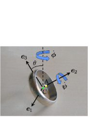
Figure 1: (Color online) (a) The geometry of a ring spun on a horizontal table. The dashed line is perpendicular to the surface of the table. The origin of the coordinate frame defined by $(\textit{{e}}_{1},\textit{{e}}_{2},\textit{{e}}_{3})$ coincides with the center of mass of the ring, point $C$. The point $A$ is the center of the upper circular edge. (b) The quasi-periodic trajectory of $\textit{{r}}_{A}(t)$ projected on the surface of the table, and in the absence of dissipative effects. We have set the initial conditions to $\theta_{0}=0.55$ rad, $\dot{\phi}_{0}=4.5$ and $\dot{\psi}_{0}=0$. All other conditions have been set to zero.

II Dynamics of rolling rings

We describe the rotation of a ring of the outer radius $R$, width $h$, thickness $w$, and mass $m$ by a set of 3-1-2 Euler angles $(\phi,\theta,\psi)$ as shown in Figure 1(a). The unit vectors $(\textit{{e}}_{1},\textit{{e}}_{2},\textit{{e}}_{3})$ are along the principal axes of the ring, $\textit{{e}}_{1}$ is always parallel to the surface of the table, and $\textit{{e}}_{2}$ is along the symmetry axis of the ring. It is remarked that the ring in Figure 1(a) has not been used to quantitatively study the kinematics and dynamics of motion. It is used only for the definition of ring geometry, and in supplementary video 1. The angular velocity of the ring thus becomes $\bm{\omega}=\dot{\theta}\textit{{e}}_{1}+(\dot{\phi}\sin\theta+\dot{\psi})\textit{{e}}_{2}+\dot{\phi}\cos\theta\textit{{e}}_{3}$. We denote the inertia tensor of the ring by I and its angular momentum with respect to the center of mass by $\textit{{L}}_{G}=\textsf{{I}}\cdot{\bm{\omega}}$. The equations of the coupled roto-translatory motion thus read

$$\textsf{{I}}\cdot\dot{\bm{\omega}}+\bm{\Omega}\times\textit{{L}}_{G} = -\textit{{r}}_{G}\times\textit{{F}},~{}~{}\textit{{r}}_{G}=(h/2)\textit{{e}}_{2}+R\textit{{e}}_{3},$$ (1)

$$m\ddot{\textit{{r}}}_{C} = \textit{{F}}-mg\left(\sin\theta\textit{{e}}_{2}+\cos\theta\textit{{e}}_{3}\right),$$ (2)

where $g$ is the gravitational acceleration, $\textit{{r}}_{C}$ is the global position vector of the center of mass, F is the boundary force at the contact point of the ring and the table, and $\bm{\Omega}=\bm{\omega}-\dot{\psi}\textit{{e}}_{2}$. Throughout our study we assume that the ring is in pure rolling condition and the constraint $\textit{{v}}_{C}=\dot{\textit{{r}}}_{C}=\bm{\omega}\times\textit{{r}}_{G}$ holds. Equations (1) and (2) can therefore be combined to obtain the evolutionary equations of angular velocities:

$$\textsf{{I}}\cdot\dot{\bm{\omega}}-m\textit{{r}}_{G}\times\left(\textit{{r}}_{G}\times\dot{\bm{\omega}}\right)=-\bm{\Omega}\times\textit{{L}}_{G}$$

$$-m\textit{{r}}_{G}\times\left(\bm{\Omega}\times\textit{{v}}_{C}\right)+mg\left[R\sin\theta-(h/2)\cos\theta\right]\textit{{e}}_{1}.$$ (3)

It is almost impossible to track the motion of the center of mass experimentally. We therefore use the center of the top circular edge of the ring (point $A$ in Fig. 1(a)), with the position vector $\textit{{r}}_{A}=\textit{{r}}_{C}+(h/2)\textit{{e}}_{2}$, for measuring the position and velocity of the ring. The velocity of point $A$ is related to the speed of the center of mass through $\dot{\textit{{r}}}_{A}=\dot{\textit{{r}}}_{C}+\bm{\Omega}\times(h/2)\textit{{e}}_{2}$. We normalize all lengths and position vectors to the mean radius $R-w/2$. Accelerations have been normalized so that the initial value of $R\dot{\phi}^{2}$ at $t=0$ equals the experimental value $\approx 20.2g$.

Integration of equation (3) for initial conditions $\dot{\theta}_{0}=0$ and $\theta_{0}>\arctan[h/(2R)]$ show that the center of mass of the ring moves on a generally quasi-periodic cycloidal orbit. A typical quasi-periodic orbit is shown in Fig. 1(b) for $R=1.025$, $h=0.88$ and $w=0.05$, which correspond to the ring in our experiments discussed below. The size of the inner turning loop of cycloids is a function of $\dot{\psi}_{0}/\dot{\phi}_{0}$ and $\theta_{0}$. Such orbits, however, are not observed in real world experiments. Spinning a wedding ring on a glass or wooden table shows that the motion is composed of two prominent phases. In the first phase, the ring spins and travels similar to the prograde turn of a coin/disk, but in contrast with a disk that continues prograde spiraling until its resting position, it abruptly makes a retrograde spiral turn before stopping (supplementary video 1). The retrograde turn does not belong to the phase space structure of equation (3), nor is it observed in spinning disks.

III Experimental results and theoretical simulations

To understand the ring dynamics, we prepared a high-speed imaging set-up and spun a ring of $R=20.66\,{\rm mm}$, $w=1\,{\rm mm}$ and $h=18\,{\rm mm}$ on a polished and waxed wooden table. The ring has been cut from a steel tube with circular cross section. We rotated and released the ring by hand, but assured that the initial conditions satisfy $\dot{\theta}_{0}\approx 0$ and $\theta_{0}>\arctan[h/(2R)]$. To trace the translational and rotational motions, we put four marks in a cross configuration at the top circular edge of the ring, and stored their coordinates (in pixels) while filming the motion (Fig. 2(a)). The centroid of these marks has the position vector $\textit{{r}}_{A}$. Figs 2a,b and supplementary video 2 show the projection of the trajectory of $\textit{{r}}_{A}(t)$ on the surface of the table for one of our experiments. The Euler angles $\theta$ and $\psi$ can be computed from the formulae $1+\sin^{2}(\theta)$=$\left(L_{13}^{2}+L_{24}^{2}\right)/D^{2}$ and $1+\sin^{2}(\psi)\left[\sin^{2}(\theta)-1\right]$=$L_{13}^{2}/D^{2}$ where $L_{13}$ and $L_{24}$ are the apparent distances between the points 1 and 3, and 2 and 4, respectively, and $D=2R-w$ is the mean diameter of the ring. Our experimental error level in computing $\textit{{r}}_{A}(t)$ has been $\approx 5\%$ because of image distortions. There are two reasons behind image distortions: perspective effects and barrel distortions (the field of view of the lens is bigger than the CCD size). Perspective distortions are functions of (i) the distance of the ring from the line of sight of the camera, and (ii) the Euler angles. The mean error threshold due to all these effects is roughly the measured value of $1-(L_{13}+L_{24})/(2D)$ after the stopping of the ring.

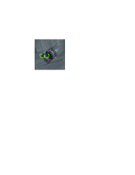
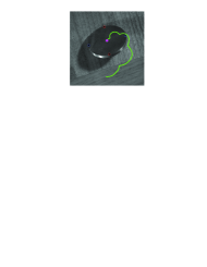
Figure 2: (Color online) (a) The first cycloidal turn of the ring. The four marks for motion tracking have been labeled by numbers 1, 2, 3 and 4. (b) The full trajectory of the center of the top circular edge, point $A$, of the ring. The ring undergoes a directional walk along the arrow. (c) The first few prograde turns of the rolling disk. (d) The trajectory of the center of mass of the disk until it reaches a small inclination angle.

The trajectories of point $A$ displayed in Figs 2(a,b) and supplementary video 2 unveil unique features of the ring’s motion. An initial prograde turning phase occurs along cycloidal curves similar to what we observe in Fig. 1(b). As time elapses, the inner turning loops of cycloids shrink and evolve to cuspy turning points that connect half-circle-shape arcs. The radii of half-circle steps decrease and the motion becomes directional along the arrow until a retrograde spiral turn begins at an inflection point.

To better distinguish the differences between the trajectories of rings and disks, we repeated our experiment for an aluminum disk of diameter $D=63.5$ mm and width $h=6.14$ mm, and recorded its trajectory. Figs 2(c,d) and the supplementary video 3 show the inspiraling motion of the disk’s center of mass. This is a generic behavior of rolling disks, regardless of their thickness Ma (2014).

Using the coordinates of the four markers on the ring, we have computed the magnitude of the velocity $\textit{{v}}_{p}=\textit{{v}}_{A}-(\textit{{v}}_{A}\cdot\textit{{e}}_{\perp})\textit{{e}}_{\perp}$, which is parallel to the surface of the table, and plotted it in Fig. 3 versus the frame number $n$. Here $\textit{{e}}_{\perp}=\sin(\theta)\textit{{e}}_{2}+\cos(\theta)\textit{{e}}_{3}$ is the unit vector normal to the surface. At the highest ($\theta=\theta_{\rm min}$) and lowest ($\theta=\theta_{\rm max}$) vertical positions of the center of mass, $\textit{{v}}_{p}$ becomes identical to $\textit{{v}}_{A}$. The envelope of the velocity profile has a shallow decline up to and after the retrograde turn, followed by a steep fall and termination of the motion.

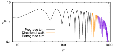
Figure 3: (Color online) The experimentally computed velocity of the ring parallel to the surface of the table. The magnitude of $\textit{{v}}_{p}$ in units of pixel/frame versus the frame number $n$. The imaging speed has been 300 frames per second, and approximately $135.6$ pixels correspond to $40.3$ mm.

We have repeated our experiments with rings of different $h/R$ ratios and observed the retrograde turn in all cases. The spiral turn is more prominent for $h/R\approx 1$ as in the ring of Fig. 2. Several mechanisms like rolling friction, slippage Kessler and O’Reilly (2002), air drag Moffatt (2000), and even elastic vibrations Villanueva (2005) can be held responsible for the phenomenon. Our numerical calculations in §IV show that the normal contact force multiplied by the coefficient of friction never exceeds the lateral frictional force, and therefore, slippage does not play any role in the occurrence of the retrograde spiral turn. Moreover, elastic vibrations may change the course of motion only if their frequencies resonate with the precession frequency $\dot{\phi}$ of the ring. We have not observed any signs of resonances in the signals of $v_{p}$ and $\dot{\phi}$. It is shown that including only the air drag fully captures the physics of the retrograde turn. In the presence of external drag torques, equation (3) takes the form

$$\textsf{{J}}\cdot\dot{\bm{\omega}} = \textit{{f}}\left(\bm{\omega},\theta\right)+\textit{{T}}_{\rm drag},$$ (4)

f $$= -\bm{\Omega}\times\textit{{L}}_{G}-m\textit{{r}}_{G}\times\left(\bm{\Omega}\times\textit{{v}}_{C}\right)$$

$$+mg\left[R\sin\theta-(h/2)\cos\theta\right]\textit{{e}}_{1},$$

J $$= \textsf{{I}}+m\left[\begin{array}[]{ccc}h^{2}/4+R^{2}&0&0\\ 0&R^{2}&-hR/2\\ 0&-hR/2&h^{2}/4\end{array}\right].$$ (8)

where J is a constant matrix, f is a vector function of the angular velocity $\bm{\omega}=\bm{\Omega}+\dot{\psi}\textit{{e}}_{2}$ and the Euler angle $\theta$, and $\textit{{T}}_{\rm drag}$ is the resultant drag-induced torque. The exact value of drag force on a general bluff body undergoing a three dimensional motion is very difficult to calculate, and is not available. In fact, the behavior of the viscous drag is so complicated that even for basic symmetric two dimensional objects under uniform transnational motion we need to entirely rely on empirical formulae Schlichting & Gersten (2000). If the bluff body in rotation is symmetric, then in order to estimate the drag moment the best approximation is to use the rotational drag coefficient and implement it on the net angular velocity vector Inarrea et al. (2003). This gives a drag moment vector in the same direction as of the angular velocity vector.

If the bluff object is not symmetric, then it is clearly not possible to define a single rotational drag coefficient for the general three-axes rotations. For a general three dimensional object, every direction of the angular velocity corresponds to a different rotational drag coefficient that needs to be found empirically. Here and as an approximation, we assume that the vector $\textsf{{J}}^{-1}\cdot\textit{{T}}_{\rm drag}$ is proportional to $\bm{\omega}$. This means rotation about a given axis does not induce angular acceleration about other axes. The rational comes from the observation that releasing the ring from a stationary initial condition with $\theta>0$ and $\bm{\omega}=\textbf{0}$ yields a simple accelerating rotation about the unit vector $\textit{{e}}_{1}$ until the ring hits the ground. Therefore, the air drag does not couple $\omega_{2}$ and $\omega_{3}$ to $\omega_{1}$. Moreover, the drag force corresponding to a pure rotation about $\textit{{e}}_{3}$ does not affect $\omega_{2}$ and $\omega_{1}$ when $\theta\rightarrow\pi/2$. The main approximation made here is for rotation about $\textit{{e}}_{2}$: as the ring rotates about $\textit{{e}}_{2}$ and undergoes a translational motion along $\textit{{e}}_{1}$ due to rolling constraint, even a small-amplitude rotation about $\textit{{e}}_{3}$ couples drag force components. Finding a more accurate model for $\textsf{{J}}^{-1}\cdot\textit{{T}}_{\rm drag}$ is beyond the scope of this study. We are not aware of any systematic method to experimentally determine drag force components near a boundary. The only reliable way is to use computational fluid dynamics (CFD) methods, which can be considered as potentially interesting problems for future works. Below it is shown that even our approximate model captures the physics of the problem very well.

We define the three rotational drag coefficients $C_{i}$ ($1,2,3$) corresponding to the three major axes of the ring and write:

$$\bm{\tau}\equiv\textsf{{J}}^{-1}\cdot\textit{{T}}_{\rm drag}=-\sum_{i=1}^{3}C_{i}\,|\omega_{i}|\,\omega_{i}\textit{{e}}_{i},~{}~{}\omega_{i}=\bm{\omega}\cdot\textit{{e}}_{i}.$$ (9)

Variants of this approach are used in naval hydrodynamics Refsnes & Sørensen (2012), flight dynamics Chudoba (2002) and low Reynolds number swimming Chattopadhyay (2008). The rotational drag coefficients $C_{i}$ implicitly depend on the Reynolds number $Re$ and the reference area of the ring exposed to airflow. If the ring was far from any wall/surface, the rotational symmetry about the $\textit{{e}}_{2}$-axis would imply $C_{1}=C_{3}$, but for rolling rings this identity does not necessarily hold. Let us define the Reynolds number as $Re=2|\dot{\textit{{r}}}_{C}|R/\nu_{a}$ where $\nu_{a}$ in the kinematic viscosity of the air. According to the velocity data of Fig. 3, the Reynolds number satisfies $Re\lesssim 800$.

Equations (4) and (9) yield $\dot{\bm{\omega}}=\textsf{{J}}^{-1}\cdot\textit{{f}}\left(\bm{\omega},\theta\right)+\bm{\tau}$. We numerically integrate this equation using the initial conditions that we measure at the first inner turning point of Fig. 2(b). In that specific position, the angular velocity $\dot{\theta}$ vanishes, and we find $\theta_{\rm min}\approx 0.55$ rad, $\phi\approx-0.38$ rad, $\dot{\psi}\approx 0$, and $\dot{\phi}=v_{A}/[R\sin(\theta_{\rm min})-(h/2)\cos(\theta_{\rm min})]\approx 4.5$. The computed initial angular velocities are dimensionless. Without loss of generality, we assume $\psi(0)=0$. The initial velocity of the center of mass is calculated using the rolling condition. To the best of our knowledge, the drag coefficients of a ring have not been measured or tabulated so far. Therefore, we constrain the parameter space $(C_{1},C_{2},C_{3})$ by generating all orbits that resemble the experimental trajectory displayed in Fig. 2(b). We find the best match between theoretical and experimental trajectories by setting $C_{1}\approx 0.03$, $C_{2}\approx 0.063$, and $C_{3}\approx 0.085$. The projection of the simulated trajectory of $\textit{{r}}_{A}(t)$ on the surface has been demonstrated in Fig. 4(a) together with the experimental trajectory. According to our computations, the topology of the trajectory is not sensitive to the variations of $C_{1}$ over the range $0.01\lesssim C_{1}\lesssim 0.1$ when the quotients $C_{1}/C_{2}$ and $C_{1}/C_{3}$ are kept constant. By varying $C_{1}$ We observe only minor differences in the location and size of the terminal spiral feature.

The actual and simulated trajectories are similar in many aspects, including 9 and 15 cycles that they make, respectively, before the directional walk and retrograde turn phases. Their major differences are the long-lived last spiral stage of the simulated trajectory, and a drift. We suspect that the observed drift has been due to (i) uncertainties in calculating the initial angular velocities through the de-projection of the images and (ii) slippage at some cuspy turning points that has slightly changed the direction of $\textit{{v}}_{A}$. For the existing discrepancy in the final spiral path we have the following explanation: as the motion of the ring slows down, $Re$ decreases and the drag coefficients increase. Consequently, the life-time of the spiral turn is shorter in reality. We would expect a better match with the experiment if the accurate profiles of the drag coefficients were known in terms of $Re$. We have repeated our experiments on glass sheets and polished steel plates, and obtained similar results. Therefore, deformation of the surface does not play a decisive role in the onset of retrograde turn.

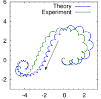
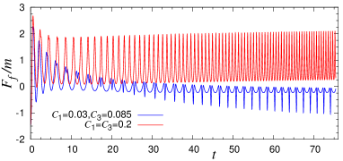
Figure 4: (Color online) (a) The projection of the simulated trajectory of $\textit{{r}}_{A}(t)$ on the surface for the same ring of Figs 1(a,b) and with $(C_{1},C_{2},C_{3})=(0.03,0.063,0.085)$. We have also reproduced the experimental trajectory of Fig. 2(b) for comparison. The motion between the initial prograde and final retrograde turning phases is directional along the arrow. (b) Same as panel (a) but for $(C_{1},C_{2},C_{3})=(0.2,0.063,0.2)$. All lengths and position vectors have been normalized to the mean radius $R-w/2$ of the ring. (c) The variation of the friction force $F_{f}$ versus time for the models of panels (a) and (b). Variables are in dimensionless units.

IV Physical origin of retrograde turn

A fundamental question is why disks do not make a retrograde turn like rings? This returns to differences in their aerodynamic properties near the ground: air can always flow through the central hole of the ring, with the drag force components $C_{i}$ ($i=1,2,3$) in all directions coming mostly from the skin friction scaled by ${\cal O}(Re^{-1/2})$ in the laminar flow conditions (with $Re\lesssim 800$) of our experiments Shevell (1989). For disks, however, air is trapped and compressed between the disk and the ground, the contribution of the form drag to $C_{1}$ and $C_{3}$ is significant, and the drag coefficients $C_{1}$ and $C_{3}\sim{\cal O}(1)$ are (almost) independent of the Reynolds number when $Re>100$ Shevell (1989). Therefore, for rolling disks we expect $C_{1}/C_{2}\gg 1$ and $C_{3}/C_{2}\gg 1$. By taking the same initial conditions for the ring in our experiments, we used $C_{2}=0.063$ and $C_{1}=C_{3}=0.2$, and found that the corresponding simulated trajectory of $\textit{{r}}_{A}(t)$ (Fig. 4(b)) is a single prograde spiral analogous to the experimentally measured trajectory of Fig. 2(d). This shows the role of enhanced drag torque about the diameter in maintaining the prograde turn.

We have found that the evolution of the lateral component $F_{f}=\textit{{F}}\cdot[\cos(\theta)\textit{{e}}_{2}-\sin(\theta)\textit{{e}}_{3}]$ of the frictional force at the contact point is the dynamical origin of the retrograde turn. The ring maintains its motion on a trajectory as in Figs 1(b) and 2(d) if the lateral force satisfies $F_{f}>0$ and supports the centrifugal acceleration needed for the prograde turn, especially when the center of mass passes through its lowest vertical position (with $\theta=\theta_{\rm max}$ and $\dot{\theta}=0$) at each cycle. At this point, the kinetic energy of the center of mass is maximum and its potential energy takes a minimum. We remark that the component $F_{1}=\textit{{F}}\cdot\textit{{e}}_{1}$ of F is also caused by friction, but it helps the rolling and cannot balance the centrifugal acceleration at turning points. Our computations (Fig. 4(c)) show that because of drag torques, a local minimum that develops on the profile of $F_{f}$ at $\theta_{\rm max}$ gradually becomes spiky and flips sign from positive to negative. As the ring experiences the strong negative kicks of $F_{f}$, the centrifugal acceleration switches sign as well, and the ring starts to revolve around a new point by retrograde turning. This process does not happen for disks, for $\omega_{1}$ and $\omega_{3}$ decay quickly due to a large $C_{1}$ and $C_{3}$, and the orbital angular momentum $\textit{{r}}_{G}\times\dot{\textit{{r}}}_{C}$ is dominated by the $\textit{{e}}_{2}$-component. Consequently, $F_{f}$ that supports the centrifugal acceleration remains positive as $\theta\rightarrow\pi/2$ (Fig. 4(c)). The coefficient of static friction for the surface on which we had spun our ring was $\mu\approx 0.4$. We computed the normal component of the contact force $F_{N}=\textit{{F}}\cdot\textit{{e}}_{\perp}$ over the entire motion of the ring and found that the inequality $\mu F_{N}>[F_{1}^{2}+F_{f}^{2}]^{1/2}$ holds at all turning points with $\theta=\theta_{\rm max}$. Therefore, slippage is not expected to play any major role in the qualitative features of the motion.

In summary, the aerodynamic interactions of spinning bodies can lead to complex, and sometimes unpredictable, results depending on the shape of the object and the initial conditions of its motion. Three well-known examples of spinning objects that significantly change their course of motion are the returning boomerang, soccer balls, and frisbees that fly along curved paths. Neither a boomerang nor a frisbee can move on curved trajectories without aerodynamic effects. Our finding for spinning rings is a new case where the frictional force and aerodynamic forces near the surface collaborate to change the course of motion.

References

- Borisov and Mamaev (2002) A. V. Borisov and I. S. Mamaev, Regular and Chaotic Dynamics 7, 177 (2002).
- Borisov et al. (2002) A. V. Borisov, I. S. Mamaev, and A. A. Kilin, Regular and Chaotic Dynamics 8, 201 (2003).
- Borisov et al. (2013) A. V. Borisov, I. S. Mamaev, and I. A. Bizyaev, Regular and Chaotic Dynamics 18, 277 (2013).
- Kessler and O’Reilly (2002) P. Kessler and O. M. O’Reilly, Regular and Chaotic Dynamics 7, 49 (2002).
- Le Saux et al. (2005) C. Le Saux, R. I. Leine, and C. Glocker, J. Nonlinear Sci. 15, 27 (2005).
- Ma (2014) D. Ma, C. Liu, Z. Zhao, and H. Zhang, Proc. R. Soc. A 470, 20140191 (2014).
- Moffatt (2000) H. K. Moffatt, Nature 404, 833 (2000).
- Easwar et al. (2002) K. Easwar, F. Rouyer, and N. Menon, Phys. Rev. E 66, 045102(R) (2002).
- Caps et al. (2004) H. Caps, S. Dorbolo, S. Ponte, H. Croisier, and N. Vandewalle, Phys. Rev. E 69, 056610 (2004).
- Leine (2009) R. I. Leine, Arch. Appl. Mech. 79, 1063 (2009).
- Bildsten (2002) L. Bildsten, Phys. Rev. E 66, 056309 (2002).
- Batista (2006) M. Batista, Int. J. Non-Linear Mech. 41, 605 (2006).
- Shegelski et al. (2009) M. R. A. Shegelski, I. Kellett, H. Friesen, and C. Lind, Can. J. Phys. 87, 607 (2009).
- Villanueva (2005) R. Villanueva and M. Epstein, Phys. Rev. E 71, 066609 (2005).
- Schlichting & Gersten (2000) H. Schlichting, and K. Gersten, Boundary-Layer Theory, Springer Science & Business Media (2000).
- Inarrea et al. (2003) M. Inarrea, V. Lanchares, V. M. Rothos, and J. P. Salas, International Journal of Bifurcation and Chaos 13(02), 393 (2003).
- Refsnes & Sørensen (2012) J. Refsnes, and A. J. Sørensen, ASME 31st International Conference on Ocean, Offshore and Arctic Engineering, paper: OMAE2012-83948 (2012).
- Chudoba (2002) B. Chudoba, Stability and Control of Conventional and Unconventional Aircraft Configurations, BoD Books on Demand (2002).
- Chattopadhyay (2008) S. Chattopadhyay, Study of Bacterial Motility using Optical Tweezers, ProQuest (2008).
- Shevell (1989) R. S. Shevell, Fundamentals of Flight, Vol. 2, Englewood Cliffs, New Jersey: Prentice Hall (1989).
- (21) See Supplemental Material at [URL will be inserted by publisher] for the real-time rolling motion of a wedding ring, which makes a terminal retrograde turn.
- (22) See Supplemental Material at [URL will be inserted by publisher] for the rolling motion of a cylindrical ring, and the trajectory of the center of its top circular face.
- (23) See Supplemental Material at [URL will be inserted by publisher] for the spin of an aluminum disk that makes a prograde spiral orbit until it stops.