GREAT3 results I: systematic errors in shear estimation and the impact of real galaxy morphology

Abstract

We present first results from the third GRavitational lEnsing Accuracy Testing (GREAT3) challenge, the third in a sequence of challenges for testing methods of inferring weak gravitational lensing shear distortions from simulated galaxy images. GREAT3 was divided into experiments to test three specific questions, and included simulated space- and ground-based data with constant or cosmologically-varying shear fields. The simplest (control) experiment included parametric galaxies with a realistic distribution of signal-to-noise, size, and ellipticity, and a complex point spread function (PSF). The other experiments tested the additional impact of realistic galaxy morphology, multiple exposure imaging, and the uncertainty about a spatially-varying PSF; the last two questions will be explored in Paper II. The 24 participating teams competed to estimate lensing shears to within systematic error tolerances for upcoming Stage-IV dark energy surveys, making 1525 submissions overall. GREAT3 saw considerable variety and innovation in the types of methods applied. Several teams now meet or exceed the targets in many of the tests conducted (to within the statistical errors). We conclude that the presence of realistic galaxy morphology in simulations changes shear calibration biases by $\sim 1$ per cent for a wide range of methods. Other effects such as truncation biases due to finite galaxy postage stamps, and the impact of galaxy type as measured by the Sérsic index, are quantified for the first time. Our results generalize previous studies regarding sensitivities to galaxy size and signal-to-noise, and to PSF properties such as seeing and defocus. Almost all methods’ results support the simple model in which additive shear biases depend linearly on PSF ellipticity.

1 Introduction

Weak gravitational lensing, the small but coherent deflections of light from distant objects due to the gravitational field of more nearby matter (for a review, see Bartelmann & Schneider, 2001; Refregier, 2003; Schneider, 2006; Hoekstra & Jain, 2008; Massey, Kitching & Richard, 2010), has emerged in the past two decades as a promising way to constrain cosmological models, to study the relationship between visible and dark matter, and even to constrain the theory of gravity on cosmological scales (e.g., Hu, 2002; Huterer, 2002; Abazajian & Dodelson, 2003; Zhang et al., 2007). Because of this promise, gravitational lensing has already been measured in many datasets, and there are several large surveys planned for the next few decades to measure weak lensing even more precisely, including Euclid (Laureijs et al., 2011), LSST (LSST Science Collaborations & LSST Project, 2009), and WFIRST-AFTA (Spergel et al., 2013), all of which are Stage IV dark energy experiments according to the Dark Energy Task Force (Albrecht et al., 2006) definitions.

The most common type of weak lensing measurement involves measuring coherent distortions (“shear”) in the shapes of galaxies. In order for the aforementioned surveys to make the most of their ability to measure these distortions with sub-per cent statistical errors, they must ensure adequate control of systematic errors. While a full systematic error budget for weak lensing includes both astrophysical and instrumental systematic errors, a problem that has occupied much attention in the community for over a decade is ensuring accurate measurements of the shear distortions of galaxies given that they have been convolved with a point spread function (PSF) and rendered into noisy images.

With the rapid proliferation of shear estimation methods, the weak lensing community began a series of blind community challenges, with simulations that included a lensing shear (known only to the organizers) that participants must measure. This served as a way to benchmark different shear estimation methods. The earliest of these challenges were the first Shear TEsting Programme (STEP1: Heymans et al., 2006) and its successor (STEP2: Massey et al., 2007a). Then it became apparent that many complex aspects of the process of shear estimation would benefit from simpler and more controlled simulations, which led to the GRavitational lEnsing Accuracy Testing (GREAT08) challenge (Bridle et al., 2009, 2010), followed by the GREAT10 challenge (Kitching et al., 2010, 2012, 2013).

Each of these challenges has been informative in its own way, illuminating important issues in shear estimation while also generating significant improvement in the accuracy of weak lensing shear estimation. For example, both the GREAT08 and GREAT10 challenges highlighted the role played by pixel noise in biasing shear estimates. While this $S/N$- and resolution-dependent “noise bias” was studied in specific contexts before GREAT08 and GREAT10 (e.g., Bernstein & Jarvis, 2002; Hirata et al., 2004), the landscape changed after GREAT08, with several more general studies (Kacprzak et al., 2012; Melchior & Viola, 2012; Refregier et al., 2012), some of which used the GREAT10 simulations as a test for calibration schemes. However, despite the progress encouraged by these challenges, there remained a number of outstanding issues in shear estimation that needed to be addressed for the community to ensure its ability to measure weak lensing in near-term and future surveys. These issues include the impact of realistic galaxy morphology: a number of studies have convincingly demonstrated that when estimating shears in a way that assumes a particular galaxy model, the shears can be biased if the galaxy light profiles are not correctly described by that model (termed “model bias”: Voigt & Bridle, 2010; Melchior et al., 2010). More generally, any method based on the use of second moments to estimate shears cannot be completely independent of the details of the galaxy light profiles, such as the overall galaxy morphology and presence of detailed substructure (Massey et al., 2007b; Bernstein, 2010; Zhang & Komatsu, 2011). Thus, the question of the impact of realistic galaxy morphology (and the way that galaxies deviate from simple parametric models) on shear estimation is important to address in a community-wide challenge. This is one of the key questions of the GREAT3 challenge.

The GREAT3 challenge was also designed to address two additional questions. One of these is the combination of multiple exposures, which is necessary to analyze the data from nearly any current or upcoming weak lensing survey. For Nyquist-sampled data this is relatively straightforward, but for data that are not Nyquist-sampled (such as some images from space telescopes), the problem is more challenging (e.g. Lauer, 1999; Rowe, Hirata & Rhodes, 2011; Fruchter, 2011). The final problem addressed in GREAT3 is the impact of PSF estimation from stars and interpolation to the positions of the galaxies. However, this paper will focus predominantly on the question of shear estimation in general and realistic galaxy morphology in particular, leaving the other questions for Paper II.

In Sec. 2, we describe how the challenge was designed and run, how submissions were evaluated, and a basic summary of the submissions that were made. We discuss the methods used by participants to analyze the simulated data in Sec. 3. For certain methods for which the teams made many submissions, we derive lessons related to those methods in Sec. 4. We then present the overall results for all teams in Sec. 5. Sec. 6 describes some lessons learned about shear estimation from GREAT3, and we conclude in Sec. 7. Finally, there are appendices with some further technical details related to the challenge simulations, and lengthier descriptions of the methods used by each team.

2 The challenge

2.1 Theoretical background

Gravitational lensing distorts the images of distant galaxies. When this distortion can be described as a locally linear transformation, then the lensing effect is described as “weak”. In this case, it relates unlensed coordinates ($x_{u}$, $y_{u}$; with the origin at the center of the distant light source) and the observed, lensed coordinates ($x_{l}$, $y_{l}$; with the origin at the center of the observed image), via

$$\left(\begin{array}[]{c}x_{u}\\ y_{u}\end{array}\right)=\left(\begin{array}[]{cc}1-\gamma_{1}-\kappa&-\gamma_{2}\\ -\gamma_{2}&1+\gamma_{1}-\kappa\end{array}\right)\left(\begin{array}[]{c}x_{l}\\ y_{l}\end{array}\right).$$ (1)

The two components of the lensing shear $(\gamma_{1},\gamma_{2})$ describe the stretching of galaxy images due to lensing, whereas the convergence $\kappa$ describes a change in apparent size and brightness for lensed objects. This transformation is often recast as

$$\left(\begin{array}[]{c}x_{u}\\ y_{u}\end{array}\right)=(1-\kappa)\left(\begin{array}[]{cc}1-g_{1}&-g_{2}\\ -g_{2}&1+g_{1}\end{array}\right)\left(\begin{array}[]{c}x_{l}\\ y_{l}\end{array}\right),$$ (2)

in terms of the reduced shear, $g_{i}=\gamma_{i}/(1-\kappa)\simeq\gamma_{i}$ in most cosmological applications. Typically it is the stretching described by the reduced shear that is actually observed. We often encode the two components of shear (reduced shear) as a single complex number, $\gamma=\gamma_{1}+{\rm i}\gamma_{2}$ ($g=g_{1}+{\rm i}g_{2}$).

The lensing shear causes a change in estimates of the ellipticity of distant galaxies. In practice, the effect is estimated statistically by measuring galaxy properties that transform in simple ways under a shear. One method is to model the galaxy image using a profile with a well-defined ellipticity, written as $\varepsilon=\varepsilon_{1}+{\rm i}\varepsilon_{2}$, with magnitude

$$|\varepsilon|=\frac{1-b/a}{1+b/a}$$ (3)

for semi-minor and semi-major axis lengths $b$ and $a$, and orientation angle determined by the major axis direction. For a population of randomly-oriented source intrinsic ellipticities, the ensemble average ellipticity after lensing gives an unbiased estimate of the shear: $\langle\varepsilon\rangle\simeq g$.

Another common choice of shape parametrization is based on second brightness moments of the galaxy image,

$$Q_{ij}=\frac{\int{\rm d}^{2}xI({\bf x})W({\bf x})x_{i}x_{j}}{\int{\rm d}^{2}xI({\bf x})W({\bf x})},$$ (4)

where ($x_{1}$, $x_{2}$) correspond to the ($x$, $y$) directions, $I({\bf x})$ denotes the galaxy image light profile, $W({\bf x})$ is an optional weight function (see, e.g., Schneider, 2006), and the coordinate origin is placed at the galaxy image center. A second ellipticity definition (sometimes called the distortion to distinguish it from the ellipticity that satisfies Eq. 3) can be written as

$$e=e_{1}+{\rm i}e_{2}=\frac{Q_{11}-Q_{22}+2{\rm i}Q_{12}}{Q_{11}+Q_{22}}.$$ (5)

The ellipticity $\varepsilon$ can also be related to the moments by replacing the denominator in Eq. (5) with $Q_{11}+Q_{22}+2(Q_{11}Q_{22}-Q_{12}^{2})^{1/2}$.

If the weight function $W$ is constant or brightness-dependent, an image with elliptical isophotes has

$$|e|=\frac{1-b^{2}/a^{2}}{1+b^{2}/a^{2}}.$$ (6)

For a randomly-oriented population of source distortions, the ensemble average $e$ after lensing gives an unbiased estimate of shear that depends on the population root mean square (RMS) distortion $\langle(e^{(s)})^{2}\rangle$ as $\langle e\rangle\simeq 2[1-\langle(e^{(s)})^{2}\rangle]g$.

See e.g. Bernstein & Jarvis (2002) for further details on commonly-used shear and ellipticity definitions.

2.2 Summary of challenge structure

Here we describe how the GREAT3 challenge was structured; more details are given in the handbook, Mandelbaum et al. (2014).

The GREAT3 challenge was designed to address how three issues affect shear estimation: (a) the impact of realistic galaxy morphology, (b) the impact of the image combination process, and (c) the effect of errors due to estimation and interpolation of the PSF. To this end, the challenge consisted of five experiments:

1. Control: Parametric (single or double Sérsic) galaxy models based on fits (Lackner & Gunn, 2012) to HST data from the COSMOS (Koekemoer et al., 2007; Scoville et al., 2007b, a) survey, meant to represent the galaxy population in a typical weak lensing survey, including appropriate size vs. galaxy flux signal-to-noise ($S/N$) relations, morphology distributions, and so on. In each image, the non-trivially complex PSF was provided for the participants as a set of nine images with different centroid offsets.

2. Real galaxy: Differed from the control experiment only in the use of the actual images from the HST COSMOS dataset instead of the best-fitting parametric models.

3. Multiepoch: Differed from the control experiment only in that each field contained six images (representing observations that must be combined) instead of one. For the space branches, the six images were not Nyquist sampled.

4. Variable PSF: Differed from the control experiment only in that the PSF varied across the image in a realistic way, and had to be estimated from star images.

5. Full: Included the complications of the real galaxy, multiepoch, and variable PSF experiments all together.

In all cases, the goal was to estimate the lensing shear. For each experiment, there were four branches, which came from the combination of two types of simulated data (ground, space) and two types of shear fields (constant, variable). For convenience, we will refer to branches by their combinations of {experiment}-{observation type}-{shear type}, e.g., control-ground-constant, and will use the unique abbreviations CGC, CGV, and so on. Of the 20 branches (five experiments $\times$ two data types $\times$ two shear types), participants could submit results for as many or few as they chose (see Mandelbaum et al., 2014, figure 5). A given branch included 200 subfields, each with $10^{4}$ galaxies on grids. To reduce statistical errors on the shear biases, galaxies were arranged such that the intrinsic noise due to non-circular galaxy shapes (‘shape noise’) was nearly cancelled out.

Submissions to the challenge were evaluated according to metrics described in Sec. 2.3. Within a branch, teams were ranked based on their best submission in that branch. Per-branch rankings were used to award teams points, which were then added up across multiple branches to give an overall leaderboard ranking. While the leaderboard ranking was necessary for the purpose of carrying out a challenge, the goal of this work is to study how teams performed and derive lessons for the future based on analysis that goes far beyond a simple ranking scheme.

There are a number of online resources related to the challenge and the simulations. The main challenge website contains overall information. The leaderboard website, linked from the main challenge website, contains the archived challenge leaderboards, and additional post-challenge boards to which submissions were made after the end of the challenge. It also links to download the GREAT3 simulations and truth tables. The GitHub site contains software to reproduce the simulated data and to analyze it using simple methods, and a wiki with information for the participants. Finally, GalSim is the simulation software that was used to make the GREAT3 simulations, and its algorithms, design, and functionality are described in Rowe et al. (2014).

Some physical effects that are not tested in the challenge include object detection, selection, and deblending, because the galaxies are located on grids; wavelength-dependent effects; instrumental and detector defects or non-linearities; star/galaxy separation; background estimation; complex pixel noise models; cosmic rays and other image artifacts; redshift-dependent shear calibration; shear estimation for galaxies with sizes comparable to the PSF; non-weak shear signals (e.g. cluster lensing); and flexion.

Appendix A contains more detailed information about some aspects of the challenge that were not in the handbook. These include Appendix A.1, on the intrinsic ellipticity distribution ($p(\varepsilon)$) of the galaxies; Appendix A.2, which describes the distributions from which the lensing shears were drawn; Appendix A.3, which presents distributions of optical and atmospheric PSF properties; and Appendix A.4, which shows the actual $S/N$ distributions for galaxies in GREAT3. The last point is particularly relevant for how pixel noise should affect shear estimates in the challenge.

Finally, the GREAT3 Executive Committee (EC) distributed example scripts to automatically process the challenge data, including shear estimation, coaddition of multi-epoch data, and variable PSF estimation. While the latter two will be discussed in Paper II, we describe the algorithms in the shear estimation example script in Appendix B.

2.3 Diagnostics

Here we describe the diagnostics used to quantify the performance of each submission to the challenge. The metrics for constant- and variable-shear branches, discussed in detail in Mandelbaum et al. (2014), were used to rank submissions. Here we briefly define the equations used.

2.3.1 Constant shear

For constant-shear simulations, each field has a particular value of shear applied to all galaxies (App. A.2). Participants submitted estimated (“observed”) shears for each constant shear value in the branch. We relate biases in observed shears $g^{\rm obs}$ to the true shear $g^{\rm true}$ using a linear model in each component:

$$g^{\rm obs}_{i}-g^{\rm true}_{i}=m_{i}g^{\rm true}_{i}+c_{i}$$ (7)

where $i$ denotes the shear component, and $m_{i}$ and $c_{i}$ are the multiplicative and additive biases, respectively. From user-submitted estimates of all $g^{\rm obs}_{i}$ in a branch, the metric calculation begins with an unweighted least-squares linear regression to provide estimates of $m_{i}$, $c_{i}$ given the true shears (in Sec. 4.8 we discuss the role of outliers in affecting the $m_{i}$ and $c_{i}$ estimates). The regression is done in a coordinate frame rotated to be aligned with the mean PSF ellipticity in each field, so that $c$ values will properly reflect the contamination of galaxy shapes by the PSF anisotropy.

Having estimated $m_{i}$ and $c_{i}$, we constructed the metric, $Q_{\rm c}$, by comparison with ‘target’ values $m_{\rm target}$, $c_{\rm target}$. These come from requirements for upcoming weak lensing experiments; we use $m_{\rm target}=2\times 10^{-3}$ and $c_{\rm target}=2\times 10^{-4}$, motivated by a recent estimate of requirements (Cropper et al., 2013; Massey et al., 2013) for the Euclid space mission. The constant-shear metric is then defined as

$$Q_{\rm c}=\frac{2000\times\eta_{\rm c}}{\sqrt{\sigma^{2}_{\text{min},{\rm c}}+\displaystyle\sum_{i=+,\times}\left[\left(\frac{m_{i}}{m_{\rm target}}\right)^{2}+\left(\frac{c_{i}}{c_{\rm target}}\right)^{2}\right]}}.$$ (8)

The indices $+$, $\times$ refer to the two shear components in the rotated reference frame described above. We adopt $\sigma_{\text{min},{\rm c}}^{2}=1~{}(4)$ for space (ground) branches, corresponding to the typical dispersion in the quadrature sum of $m_{i}/m_{\rm target}$ and $c_{i}/c_{\rm target}$ due to pixel noise. This metric is normalized by $\eta_{\rm c}$ such that methods that meet our chosen targets on $m_{i}$ and $c_{i}$ in space-based data should achieve $Q_{\rm c}\simeq 1000$. In the ground branches $Q_{\rm c}$ is slightly lower for submissions reaching target bias levels, reflecting their larger $\sigma^{2}_{\text{min},{\rm c}}$ due to greater uncertainty in individual shear estimates for ground data. However, $Q_{\rm c}$ scores are consistent between space and ground branches where biases are significant.

Given the nature of this metric definition, the uncertainty in $Q_{\rm c}$ is larger at high $Q_{\rm c}$ than at small $Q_{\rm c}$. For the level of pixel noise in the simulations from ground (space), the effective uncertainty on $Q_{\rm c}$ for $Q_{\rm c}$ values of $[100,300,500,1000]$ is $[3,28,80,328]$ ($[2,19,55,229]$).

2.3.2 Variable shear

For variable-shear simulations, the key test is the reconstruction of the shear correlation function. Submission of results for these branches begins with calculation of correlation functions by the participant. The submission consists of estimates of the aperture mass dispersion (e.g., Schneider, 2006; Schneider et al., 1998), which are constructed from two-point correlation function estimates, and allows a separation into contributions from $E$ and $B$ modes. We label these $E$ and $B$ mode aperture mass dispersions $M_{E}$ and $M_{B}$.

The submissions were estimates of $M_{E,j}$ for each of ten fields labelled by index $j$; this estimate is constructed using twenty subfields in a given field. This choice provides a large dynamic range of spatial scales in the correlation function, and thereby probes a greater range of shear signals. The $M_{E,j}$ are estimated in $N_{\rm bins}$ logarithmically spaced annular bins of galaxy pair separation $\theta_{k}$, from the smallest available angular scales in the field to the largest.

The metric $Q_{\rm v}$ for the variable-shear branches was constructed by comparison to the known, true value of the aperture mass dispersion for the realization of $E$-mode shears in each field. These we label $M_{E,{\rm true},j}(\theta_{k})$. The variable-shear branch metric is then calculated as

$$Q_{\rm v}=\frac{1000\times\eta_{\rm v}}{\sigma_{\text{min},{\rm v}}^{2}+\frac{1}{N_{\rm norm}}\displaystyle\sum_{k=1}^{N_{\rm bins}}\left|\displaystyle\sum_{j=1}^{N_{\rm fields}}\left[M_{E,j}(\theta_{k})-M_{E,{\rm true},j}(\theta_{k})\right]\right|}$$ (9)

where $N_{\rm norm}=N_{\rm fields}N_{\rm bins}$, $\sigma_{\text{min},{\rm v}}^{2}=4~{}(9)\times 10^{-8}$ for space (ground) branches, and $\eta_{\rm v}$ is a normalization factor designed to yield $Q_{\rm v}\simeq 1000$ for a method achieving $m_{1}=m_{2}=m_{\rm target}$ and $c_{1}=c_{2}=c_{\rm target}$.

The primary source of noise in the $M_{E,j}(\theta_{k})$ is pixel noise, with some residual shape noise playing a role despite the shape noise cancellation scheme. After the end of the challenge we found that a small additional source of noise comes from the interplay between the $\theta_{k}$ bin size, the galaxy grid configuration, and approximations used in the calculation of the correlation function and aperture mass dispersion in corr2. While this is a subdominant source of noise ($\sim 1/4$ of that due to measurement error), it does mean that participants will find that their $Q_{\rm v}$ results depend slightly on the ordering of galaxies in their catalog.

For the level of pixel noise in the simulations from ground (space), the effective uncertainty on $Q_{\rm v}$ for $Q_{\rm v}$ values of $[100,300,500,1000]$ is $[6,47,118,418]$ ($[5,36,91,326]$).

2.3.3 Other diagnostics

For the constant-shear branches, we have a clean way to directly study additive and multiplicative biases in the form of $m_{i}$ and $c_{i}$, where $i=+,\times$ (defined in the frame aligned with the PSF ellipticity, and at 45 degree angles with respect to that direction). However, also of interest are the $m_{i}$ and $c_{i}$ defined in the frame defined by the pixel coordinates, for $i=1,2$. In the STEP2 challenge (Massey et al., 2007a), many methods exhibited coherent differences in shear systematics along the pixel axes and at 45 degrees with respect to them, presumably due to the different effective sampling of the galaxy and PSF profiles. Since the PSF ellipticity direction has a random orientation with respect to the pixel axes, differences between $m_{1}$ and $m_{2}$ will average out, giving $m_{+}\approx m_{\times}$. Since differences between $m_{1}$ and $m_{2}$ may be interesting in understanding the performance of a method, we will use $m_{1}$ and $m_{2}$ for some of our plots.

In addition, $c_{1}$ and $c_{2}$ may be of interest. While $c_{+}$ shows the influence of PSF anisotropy, additive systematics due to PSF anisotropy will have a random sign and direction for each subfield in the pixel coordinate frame, so $c_{1}$ and $c_{2}$ have an expectation value of zero. Nonzero values may indicate selection biases with respect to the pixel direction, or asymmetric numerical artifacts.

Given the more fundamental nature of $m_{1}$ and $m_{2}$, and the need to use $c_{+}$ to identify additive PSF systematics, we also consider what we will call a “mixed metric”, $Q_{\rm mix}$, defined in analogy to $Q_{\rm c}$ (Eq. 8) as

$$Q_{\rm mix}=\frac{2000\times\eta_{\rm c}}{\sqrt{\sigma^{2}_{\text{min},{\rm c}}+\displaystyle\sum_{i=1,2}\left(\frac{m_{i}}{m_{\rm target}}\right)^{2}+\displaystyle\sum_{i=+,\times}\left(\frac{c_{i}}{c_{\rm target}}\right)^{2}}}.$$ (10)

2.4 Challenge process

During the challenge period, there were 1525 submissions with nonzero score, from 24 distinct teams. Of these, two teams were actually members of the GREAT3 EC making submissions based on simple test scripts to validate the simulations or submission process; sixteen were teams of participants; and six were teams that included at least one member of the GREAT3 EC, and were thus excluded from winning any points or the challenge itself.

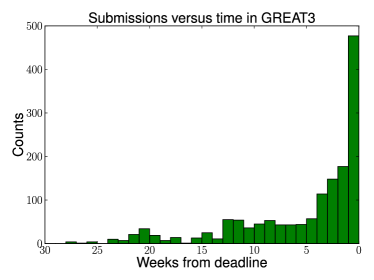
Fig. 1 shows the number of submissions to the challenge as a function of time, expressed in terms of weeks until the deadline. The first entries were submitted near the beginning of the challenge period, which ran from mid-October 2013 until April 30 2014. The submission rate was an increasing function of time particularly in the last month; the spike in entries in the last week was partly due to a relaxation of the rules on the number of entries per team per day.

Two teams entered all twenty branches, and 7/24 (30%) of the teams entered more than half the branches. Not surprisingly, many teams chose to focus on the control and realistic galaxy branches, which required the least amount of software infrastructure to participate.

Table 1 shows the results for each branch, including the winning team, the winning score (defined in Sec. 2.3), the number of participating teams, and the number of entries. As shown, a variety of teams with different methods won individual branches, rather than one team dominating everything. For all but two branches, VGV and FGV, the winning scores were $\gtrsim 800$, meaning that within the ability of the simulations to determine shear systematic errors, the winning submissions were effectively unbiased. Not only the winning team but also typically several other teams had scores in this range, representing an unprecedented quality of submissions in a weak lensing community challenge. We will discuss why the combination of variable PSF and variable shear was more difficult in Paper II.

Branch	Winning	Winning	# of	# of
	team	score	teams	entries
CGC	CEA-EPFL	1211	22 (4)	250
CGV	CEA-EPFL	1068	16 (5)	160
CSC	Amalgam@IAP	1516	16 (3)	110
CSV	Amalgam@IAP	1199	11 (4)	96
RGC	Amalgam@IAP	1121	20 (4)	195
RGV	CEA-EPFL	791	14 (4)	93
RSC	Fourier_Quad	1919	12 (3)	92
RSV	MegaLUT	1667	9 (4)	83
MGC	sFIT	1017	9 (3)	71
MGV	MegaLUT	1131	7 (2)	53
MSC	sFIT	841	6 (1)	48
MSV	CEA-EPFL	1605	6 (5)	45
VGC	sFIT	884	7 (1)	60
VGV	Amalgam@IAP	230	6 (0)	60
VSC	Amalgam@IAP	1183	4 (1)	25
VSV	sFIT	1276	4 (2)	17
FGC	sFIT	800	2 (1)	11
FGV	sFIT	379	2 (0)	17
FSC	sFIT	1184	2 (2)	17
FSV	sFIT	856	2 (2)	25

Table 1: For each branch, this table shows the winning team and its score, the number of teams that submitted to that branch (with the number having scores above 500 for the submissions analyzed in Sec. 5 shown in parenthesis), and the total number of entries in the branch.

Figure 1: Number of submissions to the GREAT3 challenge as a function of time, expressed in terms of weeks until the deadline. The rules for the number of submissions per team per day were relaxed in the final week of the challenge.

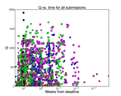
To motivate the approach we take for the analysis, Fig. 2 shows a scatter plot of metric $Q$ (either $Q_{\rm c}$ or $Q_{\rm v}$ as appropriate) as a function of time, for all submissions across all branches. Point styles indicate the team; the legend has been suppressed because our purpose is only to show that (1) there are a huge number of submissions with a wide range of performance, and (2) sometimes even within a given team, the results varied a great deal. We thus approach the analysis in two stages. Our first step, in Sec. 4, is to analyze the results for specific teams that made many submissions, to understand the trends for that method and identify a fair subset of their submissions (one per branch) to compare with those from other teams. Then, in Sec. 5, we use this fair subsample of submissions, one per team per branch, to learn lessons from the overall challenge results.

Figure 2: $Q$ for all submissions as a function of time, expressed in terms of weeks until the deadline. Later submissions by the same team that appear to perform worse than earlier submissions typically went to more challenging branches.

3 Shear estimation methods

Team	Class	Weighting	Calibration	Limitations	$N_{\rm branch}\!\!\!\!$	Rank	Exact	New	Time per
		scheme	philosophy				PSF?	software	galaxy
Amalgam@IAP	Maximum	Inverse	Ellipticity	None	16	2	Yes	Some	0.1–1 s
	likelihood	variance	penalty
BAMPenn	Bayesian	Implicit	$p(\varepsilon)$ from	Variable	2	-	Yes	Yes	$<1$ s
	Fourier		deep data	shear
EPFL_gfit	Maximum	Constant $+$	None	None	8	6	Yes	Yes	1–3 s
	likelihood	rejection
CEA-EPFL	Maximum	Various	None	None	20	3	Yes	Yes	1–3 s
	likelihood
CEA_denoise	Moments	Constant	None	None	8	-	Yes	No	0.03 s
CMU	Stacking	Constant	External	Variable	2	N/A	Yes	Some	0.03 s
experimenters			simulations	shear
COGS	Maximum	Constant	External	None	12	N/A	Yes	Yes	1 s
(im3shape)	likelihood		simulations
E-HOLICS	Moments	Constant $+$	External	None	12	8	Yes	No	1–3 s
		rejection	simulations
EPFL_HNN	Neural	Constant	None	None	7	-	Yes	Yes	2-3 s
	network
EPFL_KSB	Moments	Inverse	None	None	4	-	Yes	No	0.001-0.002 s
		variance
EPFL_MLP /	Neural	Constant	None	None	5	-	Yes	Yes	2-3 s
EPFL_MLP_FIT	network
FDNT	Fourier	Inverse	External	None	12	N/A	Yes	Some	$\sim 1$ s
	moments	variance	simulations
Fourier_Quad	Fourier	Various	None	None	6	5	Yes	No	0.001-0.002 s
	moments
HSC/LSST-HSM	Moments	Inverse	External	None	4	N/A	Yes	Some	0.05 s
		variance	simulations
MBI	Bayesian	Implicit	Inferred	Variable	4	9	No	Some	10 s
	hierarchical		$p(\varepsilon)$	shear, PSF
MaltaOx	Partially	Inverse	Self-	None	3	7	Yes	Some	0.05 s
(LensFit)	Bayesian	variance	calibration
MegaLUT	Supervised	Constant $+$	External	None	16	4	Yes	Some	0.02 s
	ML	rejection	simulations
MetaCalibration	Moments $+$	Inverse	Self-	Variable	1	N/A	Yes	Yes	0.3 s
	self-calibration	variance	calibration	shear
Wentao_Luo	Moments	Inverse	None	None	4	-	Yes	Yes	1-2 s
		variance
ess	Bayesian	Implicit	$p(\varepsilon)$ from	Variable	2	-	No	Yes	1 s
	model-fitting		deep data	shear
sFIT	Maximum	Inverse	External	None	20	1	Yes	Yes	0.8 s
	likelihood	variance	simulations
			(iterative)

Table 2: Table summarizing the methods used by teams that participated in the challenge, including basic information such as team name; class (overall type of method); weighting scheme; calibration philosophy (discussed in the text); and number of branches entered in the challenge ($N_{\rm branch}$). “Limitations” refers to types of data to which the implementation used here is not applicable without significant further development. “Rank” is the leaderboard ranking for those that received points (“-” for those that did not, and “N/A” for those that were ineligible due to participation of a GREAT3 EC member). “exact PSF?” indicates whether they used the exact PSF or an approximation to it (e.g., sums of Gaussians). “New software” indicates whether the software used to analyze the GREAT3 simulations was newly developed (“yes”), included some existing infrastructure with new software of non-trivial complexity (“some”), or was entirely pre-existing (“no”). Finally, we show the approximate processing time per galaxy per exposure (on a single core) for science-quality shear estimates. Several fields are discussed in detail in Sec. 3.

In this section, we broadly categorize and describe the methods used to analyze the GREAT3 data. Appendix C contains a more detailed description of all methods. The main aspects of the methods used by the teams in GREAT3 are summarized in Table 2, which forms the basis for the discussion in this section.

We have assigned each of the 21 teams to a “class” (listed in Table 2) that describes how the method essentially works. There are several options for the class:

1. Maximum likelihood: maximum-likelihood model-fitting methods, of which there are five.

2. Bayesian methods: there are four of these, each with different labels (e.g., “Bayesian hierarchical”, “Bayesian Fourier”, etc.) indicating differences in how they work. The “Partially Bayesian” label for MaltaOx is meant to indicate a Bayesian marginalization over nuisance parameters combined with mean likelihood estimation, rather than a fully Bayesian approach.

3. Moments: there are eight methods that work by combining estimates of galaxy and PSF moments in some way. Of these, six are real-space moments methods (called “Moments”) and two are Fourier-space moments methods (“Fourier moments”). Of the six real-space moments methods, one involves as a key aspect of the method a self-calibration scheme (“Moments $+$ self-calibration”), and that self-calibration could be extended to non-moments-based methods.

4. Stacking: a single team used image stacking.

5. Neural network and supervised machine learning (ML): three methods rely heavily on machine learning.

The table also lists the weighting scheme that was used. Here there are a few options. Several teams used constant (equal) weighting, in some cases allowing optional rejection using certain selection criteria (“Constant $+$ rejection”). Many teams used inverse variance weighting, where the variance is a combination of shape noise and measurement error due to pixel noise. In the Bayesian methods, the weights are often implicit rather than explicitly assigned. Some teams experimented with multiple weighting schemes, in which case their entry in the table is “Various”, and details are in the Appendix.

Another important entry in Table 2 is “Calibration philosophy”, which relates to how or whether a team tries to calibrate out systematic errors, versus attempting to be unbiased a priori. Here there are a few options:

1. None: These teams apply no calibration corrections.

2. External simulations: These teams generate their own simulations in order to calibrate their shears. In one case (sFIT), these are produced iteratively until they are found to sufficiently match the data that are being analyzed (“External simulations (iterative)”).

3. Ellipticity penalty term: One team, rather than applying calibrations after the fact, uses a penalty term on high ellipticity to reduce certain calibration biases. This penalty term must be calibrated in some way, making it somewhat different in nature from the next option.

4. $p(\varepsilon)$ from deep data: Some methods require an input intrinsic ellipticity distribution from deep data (or more precisely, for BAMPenn, the full distribution of unnormalized moments). This is qualitatively different from requiring external simulations, since many surveys will have a deeper subset of the data that could be used to derive this prior.

5. Inferred $p(\varepsilon)$: One team tried to hierarchically infer the $p(\varepsilon)$ and the shear from the data itself.

6. Self-calibration: Finally, two teams (MetaCalibration and MaltaOx) implemented a self-calibration scheme to derive calibration corrections from the data itself.

Table 2 also lists other useful pieces of information about these methods, as described in the caption.

4 Informative results for specific methods

Before exploring the overall results of the challenge, we first consider several methods in detail. For methods with many submissions, it is important to understand overall behavior of the method before comparing with others. For this reason, we carry out two types of tests:

1. Controlled tests of the performance of the method as a function of the various initial settings and parameter values that determine its performance, for multiple submissions in a given branch.

2. A comparison of submissions for that method across multiple branches, while holding its initial settings and parameters fixed (instead of using those that happened to give the best metric score in each branch).

These results then serve as a basis for the fair comparison between methods and across branches, which will be performed later in the paper. For all the methods discussed, see Appendix C for a more detailed description.

4.1 gfit

4.1.1 Controlled tests of variation in gfit parameters

In this section, we show results of a more detailed exploration of the gfit software used by the EPFL_gfit and CEA-EPFL teams (see method descriptions in Appendices C.3 and C.4). In particular, we investigate the dependence of the results on choices made in the course of estimating the per-object shears, or the weighting used to estimate an average shear for the entire field). Our comparison focuses on the constant-shear branches, where we have additional diagnostics such as the multiplicative and additive biases (see Sec. 2.3 for definitions).

This comparison uses the submissions from EPFL_gfit, but the results are also applicable to CEA-EPFL submissions. The factors that were considered in the comparison are the galaxy model, the postage stamp size, precision on the total flux and centroid, maximum half-light radii of the bulge and disk, filtering of the galaxy catalog, constraints on positivity of bulge and disk flux, and occasional other experiments, such as stacking the 9 PSFs in the starfield images, or running a denoising scheme.

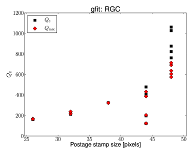
We begin by analyzing the fourteen submissions in RGC. Correlating the $Q_{\rm c}$ values with the settings that vary for these submissions, we find that the parameter that most directly predicts $Q_{\rm c}$ is the postage stamp size used for the model fitting (see top panel of Fig. 3). As shown, using the full $48\times 48$ postage stamp maximizes the $Q_{\rm c}$ score.

Figure 3: $Q_{\rm c}$ and $Q_{\rm mix}$ (top), and the bias components $m_{i}$ (middle) and $c_{i}$ (bottom), for the gfit method as a function of the postage stamp size used for modeling the galaxy images in the RGC branch. The target regions are shown as a grey shaded region, within which the vertical axis has a linear scaling; outside of the shaded region, the scaling is logarithmic. Multiple submissions with the same stamp size have slight horizontal offsets for clarity. The errorbars are correlated between the submissions, so the figure cannot be used to assess statistical significance of differences between them. See the discussion in the text for quantitative calculations of statistical significance. The $m_{i}$ and $c_{i}$ panels only show errors on a single quantity ($i=+$), for clarity.

Figure 4: $Q_{\rm c}$ and $Q_{\rm mix}$ for gfit as a function of the postage stamp size used for modeling the galaxy images in the CSC branch.

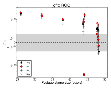
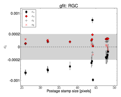
To understand this correlation, we consider the multiplicative bias as a function of postage stamp size (middle panel of Fig. 3). As shown, except for a few outliers, the multiplicative biases $m_{+}$ and $m_{\times}$ that contribute to $Q_{\rm c}$ increase from being consistent with zero to $2.0\pm 0.4$ and $2.2\pm 0.5$ per cent, respectively, as the postage stamp is reduced to half of its (linear) size. The statistical significance of the difference between the results with the maximum and minimum stamp size is more than the $3\sigma$ that it appears to be in Fig. 3; given the high ($\sim 0.75$) correlation coefficient between the submissions, the change in $m$ is detected at approximately $8\sigma$ significance.

For maximum-likelihood fitting methods, we expect a calibration bias due to the effects of noise (“noise bias”). One interpretation of the RGC results at the maximal postage stamp size is therefore a (cancelling) combination of noise bias with other potential biases, such as those expected due to an imperfect galaxy model.

As the postage stamp size is reduced, the likelihood surface for the shear estimate changes due to reduced information about the light profile, and this change will generally depend on the galaxy size and shape, postage stamp size, and the noise level. This change in the likelihood surface will in general change the location of the maximum likelihood, causing a potential bias for such methods. We refer to the resulting bias on ensemble shear estimates as “truncation bias”. For this method, the sign of the effect is apparently increasingly positive as stamp sizes decrease, though that does not necessarily have to be the case for all methods.

We can also see signs that $m_{1}$ and $m_{2}$, the calibration biases defined in the pixel coordinate system, may be related as $m_{2}\approx m_{1}+0.007$ ($1.5\sigma$ significance). A difference between the calibration bias along the pixel directions ($m_{1}$) and along the diagonals ($m_{2}$) would be consistent with the results of previous work (Massey et al., 2007a; High et al., 2007), and could plausibly be explained either by the different effective sampling of the galaxy and PSF profile along those directions, or by the fact that postage stamp itself extends further in the diagonal directions. For the maximal postage stamp size, $m_{1}$ and $m_{2}$ have opposite signs, which yields $m_{+}$ and $m_{\times}$ near zero. For this reason, $Q_{\rm c}>Q_{\rm mix}$ for the maximal postage stamp; in this case, $Q_{\rm mix}$ is a better estimator of the level of systematics in gfit.

We also investigated the additive bias and its variation with postage stamp size in the bottom panel of Fig. 3. Results consistent with zero, $c_{+}=(-1\pm 1)\times 10^{-4}$, are achieved at the maximal postage stamp size, but additive bias becomes steadily more negative until it exceeds our target value for the smallest postage stamp sizes, where $c_{+}=(-5\pm 1)\times 10^{-4}$. This result suggests that additive systematics also exhibit truncation bias (with $7\sigma$ significance after accounting for the correlation between submissions). However, the best-fitting values of $c_{1}$, $c_{2}$, and $c_{\times}$ are within the target region and statistically consistent with zero.

Fig. 3 also shows that a few submissions with large postage stamp sizes had worse than typical results. For the largest postage stamp size, these variations in $Q_{\rm c}$ are due to variations in the amount of filtering imposed on the output catalog before averaging to get a mean shear for the field. The filtering typically involves the value of the best-fit radii, the sum of the fit residuals (related to fit quality), and the $S/N$, and usually involves removing several per cent of the galaxies in each field. For the next-largest stamp size (44), the submissions with worse results involved experimenting with fit settings (e.g., allowing components with negative flux), with use of denoised images, and with stacking the nine provided PSF images instead of using just one.

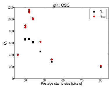
Among the space branches, CSC has many gfit entries with different postage stamp sizes, though the maximum is $80\times 80$ (out of a possible $96\times 96$). As for the ground, postage stamp size is the most important factor, with $Q_{\rm c}$ as a function of this parameter in Fig. 4. In this case, the best postage stamp size of $40\times 40$ does non-negligibly truncate the light profiles of a fair fraction of the galaxies, whereas the largest postage stamp size used ($80\times 80$) has a substantially lower $Q_{\rm c}$ due to its multiplicative calibration bias of $m_{+}=-2.0\pm 0.3$ per cent and $m_{\times}=-1.3\pm 0.3$ per cent. These biases are reduced to $m_{+}=-0.3\pm 0.3$ per cent and $m_{\times}=+0.5\pm 0.3$ per cent for the best stamp size, an $>11\sigma$ change when accounting for the strong correlation between the submissions.

The natural interpretation is that the various sources of bias in the space simulations for the largest stamp size result in a negative multiplicative bias of $\langle m\rangle\simeq-1.7\pm 0.3$% (where $\langle m\rangle=[m_{+}+m_{\times}]/2$), but a positive truncation bias cancels this out for smaller postage stamp sizes. The fact that the bias becomes more positive for smaller stamp sizes is consistent across ground and space simulations.

The potential sources of bias in the $80\times 80$ case include noise bias, some truncation bias compared to the full $96\times 96$ case, and model bias due to an inexact match between the parametric model in the simulations versus those used by gfit. In all cases, there is a detection of additive systematics, with $c_{+}$ ranging from $(7\pm 1)\times 10^{-4}$for the $80\times 80$ stamp size, to $(3\pm 1)\times 10^{-4}$ for stamps smaller than $60\times 60$. The decrease in $c_{+}$ due to truncation bias is significant at the $9\sigma$ level.

4.1.2 Fair cross-branch comparison

The best results from the gfit team used quite different postage stamp sizes for each branch. Since the galaxy populations are, in a statistical sense, consistent when comparing across all ground branches and all space branches, a fair cross-branch comparison would use consistent settings for all ground branches and for all space branches. Here we present the results of this comparison.

For ground branches, all branches except for CGC had a submission with stamp size of $32\times 32$, and CGC has one with $30\times 30$, which is close enough for this comparison. Fig. 5 shows the $Q$ values for all gfit submissions in all ground branches, particularly indicating those submissions that are part of the fair cross-branch comparison. Note that the $Q_{\rm c}$ and $Q_{\rm v}$ values do not relate to shear systematics in quite the same way, so we cannot directly compare across constant and variable shear branches. However, it is clear in general that the submissions in this fair comparison sample perform respectably ($200\lesssim Q\lesssim 600$) but do not typically include the best submission in each branch. The results for the mixed metric $Q_{\rm mix}$ in that figure (top right) for constant-shear branches actually shows consistency across branches for the selected submissions, with $250\lesssim Q_{\rm mix}\lesssim 350$.

Figure 5: Top left: Histogram of $Q$ value (either $Q_{\rm c}$ or $Q_{\rm v}$ depending on the branch) for the gfit method for all submissions in ground branches from CEA-EPFL and EPFL_gfit teams. The large dots located on the histograms indicate the submissions that are part of the fair cross-branch comparison, with the same choice of postage stamp size. Top right, bottom left, bottom right: The same, but for $Q_{\rm mix}$, $\langle m\rangle$, and $c_{+}$ (respectively), for constant-shear branches. In the bottom plots, the points have horizontal errorbars indicating their statistical uncertainty, and the shaded regions indicate the target values of $\langle m\rangle$ and $c_{+}$. Outliers have been removed from the bottom two panels so that the main part of the distribution can be clearly seen.

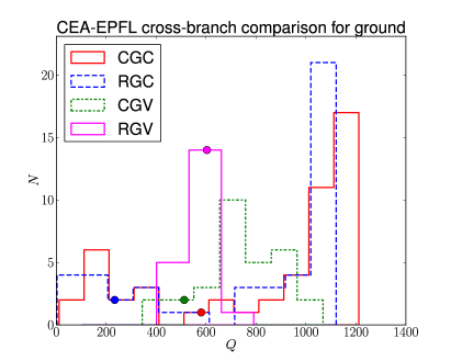
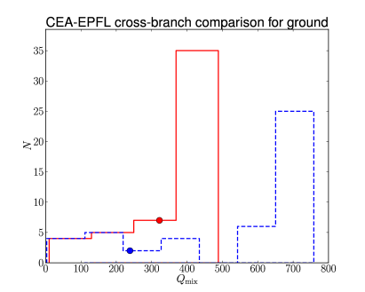
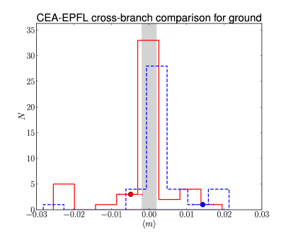
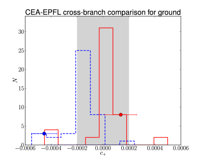
The bottom row of Fig. 5 shows the distribution of multiplicative biases averaged over both components, $\langle m\rangle=(m_{+}+m_{\times})/2$, and additive biases aligned with the PSF ($c_{+}$; no significant $c_{\times}$ was detected for this or any method) for all submissions in CGC and RGC. For $\langle m\rangle$, given the fixed gfit analysis settings, the differences between the red points in CGC and RGC indicate additional multiplicative model bias due to real galaxy morphology of $\langle m\rangle_{\rm RGC}-\langle m\rangle_{\rm CGC}=1.9\pm 0.4$ per cent. There may also be model bias in CGC due to the parametric models used by gfit not precisely matching the ones in the GREAT3 simulations. The CGC vs. RGC comparison therefore reflects only additional model bias due to real galaxy morphology, rather than all sources of model bias.

When considering the points that indicate the submissions in the fair comparison sample, the additive biases are consistent with zero for CGC but a significant detection for RGC is seen, suggestive that model bias due to realistic morphology can result in additive errors from imperfect PSF deconvolution. However, it is worth bearing in mind that the postage stamps used in this cross-branch comparison are significantly truncated. In all these ground branch submissions there will thus be some truncation bias that might interact with other biases such as model biases. The individual effects cannot be wholly isolated, but the compound effects are clear.

For space branches, the “fair comparison” submissions had postage stamp sizes of $44\times 44$, representing significant truncation compared to the full size of $96\times 96$. The fair comparison results do not exhibit the very high $Q$ values of the best submissions ($>1000$) but are, however, in the range $500<Q<800$. Comparing CSC and RSC suggests a multiplicative model bias due to realistic galaxy morphology of $\langle m\rangle_{\rm RSC}-\langle m\rangle_{\rm CSC}=0.7\pm 0.2$ per cent, but no additive model bias.

4.1.3 Summary

In summary, gfit results are significantly affected by the postage stamp size used for modeling, with small stamp sizes resulting in what we call truncation bias. This (generally positive) truncation bias can offset the negative noise bias that is a natural consequence of using a maximum-likelihood fitting method. The next most interesting factor is the filtering of the catalog to exclude galaxies on the basis of fit quality or fit parameters, with typically a few per cent of galaxies being excluded.

Results for a consistent choice of stamp size suggest differences in $\langle m\rangle$ between the control and realistic galaxy experiments of order $\Delta\langle m\rangle\simeq 1$–$2$% (greater for ground than for space) due to model bias from realistic galaxy morphology. This conclusion is based on the fact that the galaxy and data properties in these branches are the same, except for the way of representing the light profiles (parametric models vs. HST images). Thus truncation, noise, and other biases should be consistent between the two sets of results. Differences in $c_{+}$ for the control and realistic galaxy experiments depend on whether the simulated data represents a space survey or a ground survey.

We note the general point that, using this dataset, we cannot cleanly separate model bias in true isolation, as compounding interplays may exist between model bias, truncation bias, noise bias and other biases. This would be an interesting subject for future study. For the purpose of controlling for the effects found in this analysis of gfit results, in the general analysis in Sec. 5, we will use a set of gfit submissions with consistent postage stamp sizes (one set for ground, and another for space). These will be the same submissions used in Sec. 4.1.2.

4.2 Amalgam@IAP

4.2.1 Controlled tests of variation in Amalgam@IAP options

The Amalgam@IAP analysis pipeline (see Appendix C.1) has a significant number of parameters that can change. These include the postage stamp size, subpixel resolution, and order of interpolation used to combine star images for PSF estimation; the type of filtering of the galaxy catalogs; the modeling window (the maximum allowed region to use for modeling, which was either fixed to the postage stamp size or was permitted to vary with a maximum value equal to the postage stamp size); the use of regular vs. modified $\chi^{2}$ to mitigate the effects of galaxy blends (see Appendix C.1); the use of an additional penalty term on Sérsic index and/or aspect ratio, see Eq. (14); and the choice of effective shape noise $\sigma_{s}$ in the weighting used to combine individual galaxy shape estimates (see Appendix C.1.3).

Early in the challenge it was found that increasing the sampling density of both the PSF and the galaxy models ($\approx 2.5\times$ on each axis compared to the values that would automatically be set by the regular versions of PSFEx and SExtractor) significantly improved the scores, at the price of increasing computing time by an order of magnitude.

In RGC, we carried out multi-factor ANOVA to understand the most important factors determining the performance of the Amalgam@IAP team. Unfortunately, even with nearly 40 submissions, the 8-dimensional parameter space was not sampled well enough to get a clear answer. The results suggest that $\sigma_{s}$ was the most important factor determining performance, with choice of form for the $\chi^{2}$ (regular preferred over modified) and use of penalty term (penalty on aspect ratio preferred over not) being important with marginal significance.

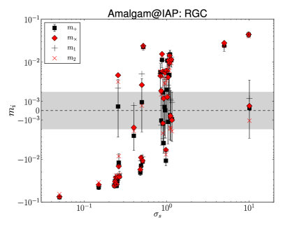
Given the importance of $\sigma_{s}$, Fig. 6 shows the variation of our metrics with this parameter.

Figure 6: From top to bottom, we show $Q_{\rm c}$, $m_{i}$, and $c_{i}$ for the Amalgam@IAP team submissions as a function of the $\sigma_{s}$ used in the weighting scheme, for all submissions in RGC. The target regions are shown as a grey shaded region, within which the vertical axis has a linear scaling; outside of the shaded region, the scaling is logarithmic. Note that the entries shown at $\sigma_{s}=10$ actually had $\sigma_{s}=\infty$, i.e., completely equal weighting for all galaxies. Multiple submissions with the same $\sigma_{s}$ have slight horizontal offsets for clarity. The $m_{i}$ and $c_{i}$ panels only show errors on a single quantity, for clarity.

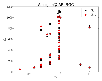
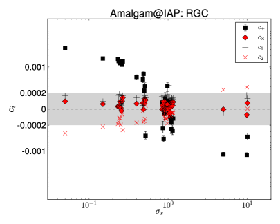
As shown in the top panel, $Q_{\rm c}$ sharply decreases for very small $\sigma_{s}$, and reaches a maximum for $\sigma_{s}\approx 1$. For infinite $\sigma_{s}$ (constant weighting), there are two submissions with quite different $Q_{\rm c}$ values, $849$ and $78$, which we discuss in more detail below.

The decrease in $Q_{\rm c}$ for very low $\sigma_{s}$ is quite interesting. As $\sigma_{s}$ approaches zero, the weighting scheme gives a strong preference to very high $S/N$ galaxies. In real data, there is no advantage to giving such a preference because of shape noise. However, in GREAT3, we have canceled out the shape noise by including 90^∘ rotated pairs, so in principle, a perfect shear estimate for just the two highest $S/N$ galaxies would perfectly determine the shear for the whole field. The low $Q_{\rm c}$ in this case implies that either the covariance matrix used for the weighting is poorly determined or has some correlation with shear direction, or that the shear estimates for high-$S/N$ galaxies are poor. The high-$S/N$ galaxies should have little noise bias, but may have model bias due to a mismatch between the input parametric models and the ones fitted by the Amalgam@IAP team. Another possible explanation relates to the adaptive selection of modeling window size (up to but not beyond the size of the input postage stamps). If the algorithm chooses too-small postage stamps for the highest-$S/N$ galaxies, it could introduce truncation biases as seen in gfit results (see Sec. 4.1). Since a similar trend in $Q_{\rm c}$ was seen in CGC, the problem is not plausibly due solely to realistic galaxy morphology. Unfortunately given the data that we have, we are unable to tease apart these effects.

The other panels in Fig. 6 show the $m_{i}$ and $c_{i}$ values as a function of $\sigma_{s}$, to explain the trends in the $Q_{\rm c}$ plot. For very low $\sigma_{s}$ (upweighting the high $S/N$ galaxies), the multiplicative biases can be as bad as $-7.6\pm 0.5$ per cent, with a very high detection significance for the trends in $m_{i}$. For constant weighting, the submission with near-zero $m_{i}$ and $c_{i}$ includes a penalty term on the aspect ratio, whereas the poorly-performing submission does not (giving a $10\sigma$ change in $m_{i}$). In the bottom panel, as $\sigma_{s}$ goes from 0.05 up to 1 and finally to $\infty$ (corresponding to strong $S/N$ upweighting, weighting with a substantial shape noise term, and constant weighting, respectively), $c_{+}$ goes from $(3.2\pm 0.2)\times 10^{-3}$, to consistent with zero, to negative values, $(-4\pm 1)\times 10^{-4}$. The statistical significance of these changes is $>10\sigma$. This suggests that $c_{+}$ for this method is positive (negative) for the high- (low-) $S/N$ galaxies.

We now address the issue of the penalty term on aspect ratio, another parameter of interest that causes highly significant changes in multiplicative and additive biases as discussed above. The idea of the penalty term is that for galaxies that have low $S/N$ and poor resolution, the ellipticity is so poorly determined that there is a very large tail to high ellipticity (which is a manifestation of noise bias). Hence the idea is to penalize high ellipticity values by adding a term to the $\chi^{2}$, which will have little effect on high-ellipticity objects with high $S/N$. This was important particularly for fields with poor seeing and/or substantial defocus that enlarged the PSF. An example is shown in Fig. 7. The top panel shows the fitted ellipticity distribution in a good-seeing (blue) and poor-seeing (red) field in GREAT3 without the penalty term, and the bottom panel shows the same when using the penalty term on aspect ratio. The distribution for the poor-seeing image has a pronounced high-ellipticity tail that is nearly removed by the penalty term, yet the shape of the distribution in the good-seeing image is less altered by the addition of this term.

Figure 7: Fitted ellipticity distributions for the Amalgam@IAP team for a good-seeing (blue) and poor-seeing (red) subfield in GREAT3, in the CGC branch. The top (bottom) panel shows the results without (with) a penalty term on aspect ratio.

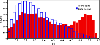
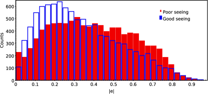
In some sense, the addition to the term in the $\chi^{2}$ is equivalent to multiplying the likelihood, i.e., imposing a prior on the ellipticity. It seems that this is a way to remove or reduce noise bias in all fields (with stronger impact on those that have poor seeing), eliminating the need for explicit calibration factors. For GREAT3, the best value of shape noise $\sigma_{s}$ to use in the weighting scheme and the form of the penalty term to use in the $\chi^{2}$ was clearly shown to do an excellent job at shear estimation for the particular $p(\varepsilon)$ and galaxy property distributions used here. However, it is unclear whether these results would necessarily be consistently reproducible for other datasets with different intrinsic $p(\varepsilon)$, or those with a $p(\varepsilon)$ that correlates with other galaxy properties in a way that is not reproduced here. For this reason, further simulations would be needed to evaluate the generality of this procedure for real data with a variety of properties, and confirm that the exact $\sigma_{s}$ and form of the penalty term gives similar results in cancelling out noise bias.

4.2.2 Fair cross-branch comparison

For the Amalgam@IAP team, it was difficult to identify a single group of settings used for all branches. Instead, four groups of settings with submissions in a few branches were identified:

1. $\chi^{2}$ penalty term on aspect ratio $\theta_{\rm aspect}$; $\sigma_{s}=0.5$ for weighting.

2. $\chi^{2}$ penalty term on $\theta_{\rm aspect}$; uniform weighting ($\sigma_{s}=\infty$).

3. $\chi^{2}$ penalty term on $\theta_{\rm aspect}$ and Sérsic index $n_{s}$; $\sigma_{s}=0.5$.

4. No priors on model parameters; $\sigma_{s}=0.5$.

The settings also differed in minor ways that have little impact on performance.

Fig. 8 shows histograms of $Q_{\rm c}$, $\langle m\rangle$, and $c_{+}$ values for all Amalgam@IAP submissions in all constant shear branches, also indicating those submissions with the aforementioned consistent settings with points. As shown, for branches that include submissions with setting 1, that submission is typically among the best in the branch, with RSC being the exception to this rule. This is consistent with our previous results indicating that $\sigma_{s}\sim 0.5$ and the $\chi^{2}$ penalty term on aspect ratio were important factors affecting the results.

Comparing the results for setting 1 and 2 in RGC, the only constant shear branch to include submissions with both settings, their performance seems quite consistent with each other. However, in variable shear branches (not shown), setting 1 leads to better performance, confirming the importance of the weight including both shape and measurement noise rather than using equal weighting.

Comparing settings 1 and 3, we see that for CGC, setting 1 leads to better performance due to a substantially smaller calibration bias. This suggests that use of a Sérsic $n$ penalty term is unimportant or perhaps even harmful, though its impact is somewhat less on variable shear branches (not shown). This finding may simply reflect the fact that the variable shear metric is less sensitive to multiplicative bias $m$.

Finally, settings 1 and 4 gave similar results, with comparable $m_{i}$ and $c_{i}$. While the use of penalty terms on $\theta_{\rm aspect}$ is helpful, that is especially true for higher $\sigma_{s}$ than the value used here.

Figure 8: Top: Histogram of $Q_{\rm c}$ values for all submissions from the Amalgam@IAP team for constant shear branches. The colored points indicate submissions that are part of the fair cross-branch comparisons with consistent settings, with the four settings described in the text indicated with different shaped points. Middle, bottom: The same, but for $\langle m\rangle$ and $c_{+}$. The points have horizontal errorbars indicating their statistical uncertainty, and the shaded regions indicate the target values of $\langle m\rangle$ and $c_{+}$. Outliers have been removed from the bottom two panels so that the main part of the distribution can be clearly seen.

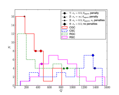
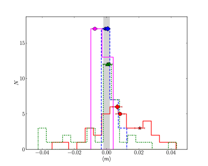
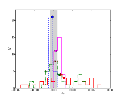
In general, the results for these fairly chosen sets of submissions are worse in CGC than in RGC. The primary reason is an average multiplicative bias of $\langle m\rangle=0.8\pm 0.2$ per cent in CGC, while $\langle m\rangle$ is consistent with zero in RGC. Since the simulation designs in the control and realistic galaxy experiments correspond apart from galaxy morphology, this difference between CGC and RGC suggests a model bias due to realistic galaxy morphology that is of that order. This bias may be canceled out by some other bias in RGC (perhaps noise bias, truncation bias, or residual model bias due to mismatch between input and output parametric models). In contrast, the additive systematics for CGC vs. RGC (setting 1) are consistent within the errors. For space branches, the multiplicative biases differ for RSC and CSC by $\langle m\rangle_{\rm RSC}-\langle m\rangle_{\rm CSC}=0.80\pm 0.15$ per cent, suggesting that model bias due to realistic galaxy morphology has a similar magnitude for both space and ground data.

4.2.3 Summary

Here we summarize the key lessons from analysis of the Amalgam@IAP results. First, the main factors that determine performance are the magnitude of shape noise used in the weighting scheme ($\sigma_{s}$) and the use of a penalty term on the aspect ratio to reduce the incidence of spurious highly elliptical, lower $S/N$ and resolution objects. Using the best choices for these parameters in all branches resulted in overall good performance, though with hints of a model bias for ground and space data due to realistic galaxy morphology that is slightly below a per cent. Also, strong variation in $c_{+}$ with the weighting scheme suggests that the additive systematics are a strong function of the galaxy $S/N$.

Because of the importance of $\sigma_{s}$ and penalty terms in determining performance, for the overall analysis and comparison with other methods, we use a set of submissions with the same value of $\sigma_{s}=0.5$ and a penalty term on the aspect ratio, with small variations in other less important parameters.

4.3 MegaLUT

4.3.1 Controlled tests of variation of parameters

The MegaLUT team (see Appendix C.17) made many submissions with varying choices related to the learning sample generation, shape measurement, input parameters for the artificial neural network (ANN), architecture of the ANN, and finally the rejection of faint or unresolved galaxies. Here we will explore the dependence of their results on these choices.

First, we consider the filtering of the catalogs, comparing four submissions to CGC that used the same settings for all parameters except the filtering. The $m_{i}$ and $c_{i}$ values for these four submissions are shown in Fig. 9, with the $Q_{\rm c}$ values indicated in the legend.

Figure 9: Top: $m_{i}$ values for four MegaLUT submissions in CGC with different choices for how catalogs were filtered, but otherwise the same settings. Bottom: $c_{i}$ values.

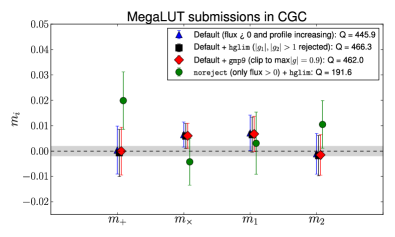
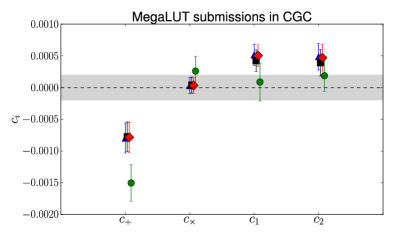
As shown, the results for the top three options (all with default filtering for positive flux and profile increasing) give very similar results, regardless of other choices like rejection based on maximum shear values, or clipping large shears (setting them to a maximum value of $0.9$). However, removing the default filtering and only rejecting based on $|g_{1}|$ or $|g_{2}|>1$ gives significantly worse $Q_{\rm c}$. This is due to both $m_{i}$ and $c_{+}$ increasing in magnitude. This submission is only mildly correlated with the others, and the $m_{i}$ and $c_{i}$ changes are only marginally significant ($2\sigma$). On a minor note, there is a $2$–$3\sigma$ hint of non-zero $c_{1}$ and $c_{2}$, which (if real) may reflect asymmetry in selection criteria. Note that the default filtering option removes typically $<1$ per cent of the galaxies.

The next test was on CSC, comparing two otherwise similar submissions with different choices at the training stage. The training sample shears were uniformly distributed with $|g|<1$ and with $|g|<0.7$. The $Q_{\rm c}$ values were $289$ and $228$ respectively, primarily because of a larger magnitude of the (negative) calibration bias in the latter case. This change in $m$ is not very statistically significant ($<2\sigma$), which is interesting because it suggests a lack of sensitivity to this aspect of the training.

Also in CSC, we compare two submission that used different statistics of the image to describe the shape. In one submission, the adaptive moments routines in GalSim were used, effectively fitting the image to an elliptical Gaussian; the other submission used the moments of the autocorrelation function (ACF, van Waerbeke et al., 1997) of the image. The results are shown in Fig. 10.

Figure 10: Top: $m_{i}$ values for two MegaLUT submissions in CSC with different methods of measuring galaxy shapes, but otherwise the same settings. Bottom: $c_{i}$ values.

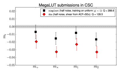
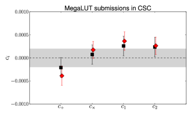
The $Q_{\rm c}$ values are $289$ and $129$, respectively, due to a $3\sigma$ difference in $m_{i}$ values (the significance is larger than it appears on the plot due to correlations between the submissions). Use of the ACF gives a more negative calibration bias of $\langle m\rangle=-2.5\pm 0.5$ per cent, compared to $\langle m\rangle=-1.1\pm 0.5$ per cent without its use. Apparently the ACF is not an unbiased way of compressing the information in the image, consistent with what was seen for two methods using the ACF in GREAT10 (Kitching et al., 2012).

A final study performed in CSC relates to other ways of filtering the catalogs after shear estimates have been made, comparing the results of the default filtering with two other options: excluding small objects, and using convex hull peeling (Eddy, 1982). The exclusion of small objects changes $m_{i}$ and $c_{i}$ only slightly. However, convex hull peeling gives substantially worse results that are also noisier, with $Q_{\rm c}$ reduced from around $300$ to $113$, and $\langle m\rangle$ going from $-1.1\pm 0.5$ to $3\pm 1$ per cent ($4\sigma$ significance).

For RSC, we compared two submissions with different training options. In one case (“half noise”), the training set images had noise that was half the level in the GREAT3 images; in the other case, it was “low noise”, $1/10$ the level in the GREAT3 images. Fig. 11 shows that the latter gives significantly better performance, $Q_{\rm c}=221$ instead of $139$.

Figure 11: Top: $m_{i}$ values for two MegaLUT submissions in RSC with different choices for how much noise to include in the training sample. Bottom: $c_{i}$ values.

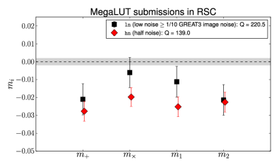
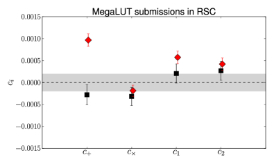
The “half noise” case has slightly worse $m_{i}$ values, and substantially worse additive systematics of $c_{+}=(10\pm 1)\times 10^{-4}$ vs. $c_{+}=(-3\pm 2)\times 10^{-4}$ in the low noise case, a $5\sigma$ difference given the correlations between the submissions). The increase in $m_{i}$ with increasing noise in the training sample images could be due to the resulting noisiness in the input features of the ANN training. This noisiness smears out any sharp structures that the ANN regression should fit, leading to biased ANN predictions. We speculate that the effects on $c_{+}$ may relate to errors in centroiding that are larger along the PSF direction somehow being amplified if the training sample is also noisy, but this effect requires further study to fully understand.

The final test in RSC relates to the use of clipping the shears, meaning setting those galaxies with estimated $|g|>g_{\rm clip}$ to $|g|=g_{\rm clip}$ instead of using the estimated value. We compare two submissions with $g_{\rm clip}=0.6$ and $0.9$ and otherwise similar settings, and find $Q_{\rm c}$ values of 76 and 105, respectively. While the additive systematics are virtually identical, the submission with stronger clipping has worse calibration bias ($\langle m\rangle$ is more negative: $-4.5\pm 0.5$ per cent instead of $-3.0\pm 0.5$ per cent, significant at more than $20\sigma$ given the high correlation between the submissions). Not surprisingly, aggressive clipping of shear magnitudes biases the estimated cosmological shear low.

4.3.2 Fair cross-branch comparison

We also show results for a fair cross-branch comparison using similar settings for the training set, filtering, and other parameters of interest. In this case, $|g|$ in the simulations was uniformly distributed in a unit disk of radius $0.7$; the simulations had half the noise of the GREAT3 simulations; galaxies with estimated $g_{1}$ or $g_{2}$ with magnitude larger than $1$ were rejected, but no other rejection scheme was used; and shears were clipped to a maximum of $0.8$. As for the other cross-branch comparisons, we show histograms of all submissions and points indicating the ones in the fair comparison set, in Fig. 12.

Figure 12: Top: Histograms of $Q$ values (either $Q_{\rm c}$ or $Q_{\rm v}$ depending on the branch) for the MegaLUT team. The colored points indicate the submissions that are part of the fair cross-branch comparison with consistent settings. Middle, bottom: The same, but for $\langle m\rangle$ and $c_{+}$ (respectively), which involves using constant-shear branches only. The points have horizontal errorbars indicating their statistical uncertainty, and the shaded regions indicate the target values of $\langle m\rangle$ and $c_{+}$. Outliers have been removed from the bottom two panels so that the main part of the distribution can be clearly seen.

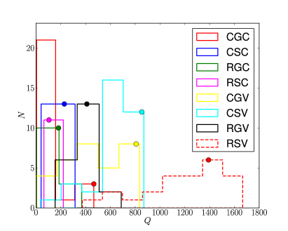
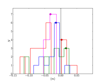
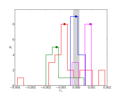
As shown in the top panel of Fig. 12, the MegaLUT submissions in the cross-branch comparison set are typically among their top submissions. The top values of $Q_{\rm c}$ are in the range $200$–$700$, whereas the top values of $Q_{\rm v}$ are in a higher range, $400$–$1400$. For all combinations of (experiment, observation type) to which this team submitted, the results for variable shear were better than for constant shear. This may reflect the fact that the best results typically had $\sim 1$–$2$% multiplicative calibration biases, to which $Q_{\rm c}$ is substantially more sensitive than $Q_{\rm v}$. For constant-shear branches, the results for the mixed metric $Q_{\rm mix}$ were very similar to those for the standard $Q_{\rm c}$. Another interesting trend across branches is that, with the exception of RSV, MegaLUT did better in the control experiment than in the realistic galaxy experiment, perhaps reflecting a preference for the parametric models used to generate the training sample (which we explore in detail in Sec. 5.3).

The middle panel of Fig. 12 shows $\langle m\rangle$ averaged over components. As shown, for both control and realistic galaxy experiments, the multiplicative bias $\langle m\rangle$ is typically positive for ground-based data (around $1$%) and negative for space-based data ($-1.5$% to $-3$%). The magnitude of the bias is slightly larger for the realistic galaxy experiment than for the control experiment. The differences are of $\langle m\rangle_{\rm RGC}-\langle m\rangle_{\rm CGC}=1.4\pm 0.4$ per cent for ground and $\langle m\rangle_{\rm RSC}-\langle m\rangle_{\rm CSC}=-1.7\pm 0.3$ per cent for space. This may reflect differences in model bias from realistic galaxy morphology.

Finally, the bottom panel of Fig. 12 shows the additive bias $c_{+}$. We see a statistically significant difference in additive biases for the control and realistic galaxy experiments, which is partly responsible for the worse performance in realistic galaxy branches compared to control branches. This is a manifestation of model bias due to realistic galaxy morphology.

4.3.3 Summary

To summarize the MegaLUT results, we find that good results required identification and rejection of a small fraction of problematic galaxies. Use of the image autocorrelation function led to substantially worse performance than use of the adaptive moments (from a fit to an elliptical Gaussian, using code in GalSim). An attempt to use convex hull peeling led to substantial calibration biases and overall noisiness. Use of training images with $1/10$ (rather than $1/2$) the noise level of GREAT3 reduced the additive systematic errors. Finally, clipping the shears substantially (to a maximum value of $|g|=0.6$) led to negative calibration biases and overall worse performance. The MegaLUT method had overall better performance in variable-shear branches due to the pervasive $\sim 1$ per cent calibration biases, which hurt their performance preferentially on the constant-shear branches. This multiplicative calibration bias has opposite signs for ground and space data (but similar magnitude). We saw hints of additive and multiplicative model bias due to realistic galaxy morphology, which we will explore in more detail in Sec. 5.3.

While using low noise training data led to improved performance, there was not a fair set of submissions across all branches that used low noise. Thus, for the overall analysis in Sec. 5, we will use a set of submissions with half noise. However, it is important to bear in mind that this degrades the performance of the method.

4.4 Fourier_Quad

For Fourier_Quad (see Appendix C.13), the key difference between submissions relates to the weighting scheme used when combining per-galaxy shear estimates. Three options were used for GREAT3:

• No explicit weighting: Since the galaxy light profile amplitudes scale with the flux, if this is not divided out, a lack of explicit weighting corresponds to implicit weighting by $(S/N)^{2}$. In GREAT3 this improves performance given our use of shape noise cancellation, in a way that is not viable in real data where shape noise does not cancel.

• Identifying the pairs of 90^∘-degree rotated galaxies and dividing the $G_{1}$, $G_{2}$ and $N$ for each object (see Appendix C.13) in the pair by the squared galaxy flux. This weighting scheme is also not viable for real data.

• Dividing the power spectrum of the galaxy image by the square of the galaxy flux, which corresponds to effectively unweighted per-galaxy shear estimates.

For the constant-shear branches, higher scores were achieved using the first weighting scheme, followed closely by the second. For example, in CGC, the top $Q_{\rm c}$ scores using the first two weighting schemes were 1202 and 1122, respectively; in RGC, 888 and 764; in CSC, 1318 and 1245; in RSC, 1919 and 1726. Clearly the performance was excellent with both weighting schemes, with $m_{i}$ and $c_{i}$ values at or near the target range. However, since these are not a viable approach in real data, all comparisons with other methods (in Sec. 5) will use the third weighting scheme.

For two reasons, Fourier_Quad did not get high scores in variable-shear branches. First, unlike most of the other methods, the shear estimators of Fourier_Quad do not directly correspond to galaxy ellipticities, so the method does not get the full advantage of having zero intrinsic $E$-mode correlation in variable-shear branches. Second, the way of calculating shear correlation functions in Fourier_Quad is still sub-optimal, as described in App. C.13. Since we wish to use results that correspond to what would be used in real data, we do not use their variable-shear submissions for our overall analysis.

4.5 sFIT

For the sFIT team (see Appendix C.21), multiple submissions in each branch reflect more complete or sophisticated sets of simulations from which to derive multiplicative and additive calibration factors to apply to per-galaxy shear estimates. Thus, it is generally the case that the most fair submission to use in each branch is the one that was submitted last, except in a few branches with some experimental submissions at the end.

However, comparing the results for individual submissions within a branch provides information about the sizes of various biases. For example, in CGC, the $Q_{\rm c}$ value changed from 579 to 974 from the first to the last submission. The initial attempt came from applying calibration based on simulations that approximately matched distributions in size, Sérsic index, and noise level, but with Gaussian PSFs rather than the real PSFs. Despite the simplifications in the initial simulations used to derive the calibration factors, the best-fitting $m_{i}$ values were $\sim 0.5\pm 0.5$ per cent in each component, and $c_{+}$ was consistent with zero. It is likely that the calibration correction in this branch is dominated by noise bias corrections. Later improvements involved oversampling the Sérsic profiles, a better PSF model (double Gaussian, which is still not as complex as the real PSF model), and improved Sérsic $n$ distribution based on CSC, which primarily improved the score by reducing the multiplicative bias to $0.3\pm 0.5$ per cent. For the final submission, the average multiplicative calibration factor over all the subfields (with a different value of calibration depending on the PSF FWHM) was approximately $1.06$, and the magnitude of the typical additive bias correction (which depends on the PSF FWHM and its ellipticity) was of order $5\times 10^{-4}$. The final results in CGV, with $Q_{\rm v}=841.4$, resulted from directly applying the calibration factors from the final submissions to CGC, as is appropriate given the similarities in branch design.

In CSC, the initial basic calibration (derived in a rough way as for CGC) led to $Q_{\rm c}=698$. Further iterations involved narrowing distributions of Sérsic $n$ and $S/N$ (because the original ones from fits to the GREAT3 data had an unphysical tail due to noise), and ultimately achieved $Q_{\rm c}=920$. The processing used a $45\times 45$ postage stamp, not the full $96\times 96$, which should result in truncation bias as in Sec. 4.1. However, since the calibration simulations also use small postage stamps, the truncation bias should be automatically corrected. The magnitude of the total multiplicative bias correction for this final submission was approximately 1.02, with an additive bias correction of order $-2\times 10^{-4}$.

In the realistic galaxy experiment, we first consider RGC. Interestingly, the first submission (with $Q_{\rm c}=305.4$) used calibrations derived from simulations with real galaxy images in GalSim. However, the next attempt directly used the calibrations from CGC, which do not include realistic galaxy morphology, and achieved $Q_{\rm c}=806.9$. This change tells us that for the sFIT method of fitting Sérsic profiles, the model bias due to realistic galaxy morphology is not very large in ground-based data, because it is in principle uncorrected in these results. After modifying the simulation inputs to better match the $p(\varepsilon)$ and size distribution in RGC, the results were as high as $1003$, with $\langle m\rangle=0.2\pm 0.5$ per cent, and $c_{+}=(1\pm 1)\times 10^{-4}$. This suggests that residual model bias due to realistic galaxy morphology is only important at the $10^{-3}$ level for this method, compared to $10^{-2}$ for the methods discussed previously. The best-scoring submissions in RGV used the calibration from RGC.

In RSC, interestingly, simulations based on real galaxy images were necessary to improve $Q_{\rm c}$ above $\sim 350$. Use of COSMOS images led to an immediate boost of $Q_{\rm c}$ to $759$ in the first attempt, which is a statistically significant change arising from $\langle m\rangle$ changing from $-0.9\pm 0.3$ per cent to $-0.2\pm 0.3$ per cent, with nearly the same additive bias, $c_{+}=(5.2\pm 0.8)\times 10^{-4}$. The significance of the change in $\langle m\rangle$ is $>20\sigma$ due to the very high correlation between the submissions. This suggests a statistically significant, sub-percent model bias due to realistic galaxy morphology for this method in space data. Further attempts to improve the simulated $p(\varepsilon)$ to match the GREAT3 simulations led to additional improvements to $Q_{\rm c}=825$, with the additive bias remaining unchanged. One possible cause for this residual bias is that the calibration simulations did not use a fully realistic PSF, which could result in slightly incorrect additive bias corrections.

4.6 MBI

As described in Appendix C.15, the MBI team made submissions using a few variations of their method.

For the Optimal Tractor and Sample Tractor, they used the maximum-likelihood estimate of the lensed ellipticity and the average of samples from the posterior PDFs (respectively) to derive the mean shear for the field, typically with similar performance. For example, in CGC, the scores for the Optimal Tractor submissions were 15 and 53, reflecting multiplicative biases of $24$ and $8$ per cent, and non-negligible additive systematics. The results for the Sample Tractor submissions were in the same range. The results in RGC for these two cases were worse than in CGC.

However, hierarchically inferring the intrinsic ellipticity distribution using importance sampling from the posterior PDF for the mean shear, with a Gaussian $p(\varepsilon)$ in each component, improved scores by factors of $\sim$ 3-10 in the ground branches. These score improvements come from a decrease in multiplicative biases to the range $1$–$3$%, and a reduction in additive systematics to within the target range. The exception to this trend is CSC, where the use of hierarchical inference did not yield significant improvement ($Q_{\rm c}$ scores were typically in the range 90–200 regardless of method). However, there the assumption that the PSF can be described as a sum of three Gaussian components is more dubious than in the ground branches, so PSF modeling may be the key limitation in that branch.

The results in the ground branches for the Important Tractor (hierarchical inference) submissions suggest that this new method may indeed be able to reduce some intrinsic limitations of maximum-likelihood fitting methods (e.g., noise bias). Noise bias primarily arises when transforming a probability distribution for a galaxy shape estimate into a single point estimator. Combining the probability distributions for all galaxies (resulting in increased $S/N$) and applying a hierarchically inferred prior $p(\varepsilon)$ yields improved results.

The submissions from MBI included several variants of the hierarchical inference. The first, called “multi-baling” (hierarchically inferring the $p(\varepsilon)$ common to five subfields), led to some improvements in scores, up to a factor of two. In contrast, using the deep fields to infer the $p(\varepsilon)$ did not result in an improvement in $Q_{\rm c}$ over hierarchical inference assuming an uninformative hyper-prior. Finally, the MBI team made submissions with informative prior PDFs on the lensing shear, with four different values that seem to bracket a peak in $Q_{\rm c}$ in the CGC branch. The highest $Q_{\rm c}$-scores obtained this way (in CGC and MGC) were around a factor of four higher than that for an asserted uniform prior PDF for the shear components. For example, with their wide, default, narrow, and narrower assumed values for $\sigma_{g}$, the $Q_{\rm c}$ values were $94$, $146$, $301$, and $24$, corresponding to multiplicative biases in the range $4$%, $3$%, $-0.4$%, and $-14$%, respectively. In GREAT3 constant-shear simulations, the true $p_{\text{true}}(|g|)\propto|g|$ (see App. A.2), whereas the MBI team used Rayleigh distributions. Their “wide” and “narrower” distributions are particularly mismatched in shape to the true one, so the poor $Q_{\rm c}$ scores are not surprising.

After the challenge, the MBI team investigated inferring the optimal value of $\sigma_{g}$ from the data directly (as opposed to from $Q_{\rm c}$). This yields a factor of two improvement over an asserted uniform prior PSF for the shear components. It is unclear how much better one can do in this way on GREAT3 simulations because of the unusual $p(|g|)$, which differs from the functional form chosen by the MBI team (and makes sense for real data).

For the overall analysis in Sec. 5, we use the MBI results with hierarchical inference. While multi-baling and using deep fields to get the $p(\varepsilon)$ may become helpful in future, they were not fully explored in GREAT3, so we do not use them for the overall comparison.

4.7 COGS

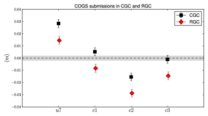
The COGS team made a number of submissions, using the im3shape algorithm (Zuntz et al., 2013), that are described in Appendix C.7. The submissions that used input settings and methodology suitable for scientific analysis are labelled u7, c1, c2, and c3. The labels c1 – c3 denote three different schemes used to calibrate for multiplicative biases that are expected in Maximum-Likelihood shape estimation. No correction was applied for additive bias.

In Sec. 5, and thereafter, where we wish to draw fair comparisons between branches and between methods, only COGS submissions that used the c3 calibration are used. This choice is made as c3 comes closest to the approach that would be adopted when applying im3shape to real data (see Appendix C.7).

The different submissions make it possible to test for the effect of different choices made in the noise bias calibrations, and to test for model bias due to realistic galaxy morphology by comparing CGC and RGC. Fig. 13 shows the significant impact of noise bias calibrations on $\langle m\rangle=(m_{+}+m_{\times})/2$ for COGS submissions to CGC and RGC. The c3 calibration, derived from the deep data in CGV but with some outlier rejection in deep field fits (see Appendix C.7), controls multiplicative biases in CGC to within statistical uncertainties. For u7, i.e. without any attempt to calibrate multiplicative bias, we find $\langle m\rangle=2.8\pm 0.3$ per cent for CGC and $\langle m\rangle=1.4\pm 0.3$ per cent for RGC. These results represent a combination of noise, model, and other biases in the uncalibrated COGS submissions.

For each pair of submissions grouped by calibration strategy, we also find a consistent difference in the level of multiplicative bias between CGC and RGC results: $\langle m\rangle_{\rm RGC}-\langle m\rangle_{\rm CGC}=-1.4\pm 0.5$ per cent. This difference in $\langle m\rangle$ can be interpreted as a difference in model bias due to realistic galaxy morphology, for the im3shape galaxy model chosen by the COGS team. It is similar in magnitude to the effect found in other model-fitting methods.

Figure 13: Averaged multiplicative bias $\langle m\rangle=(m_{+}+m_{\times})/2$ for COGS submissions to CGC and RGC, under differing schemes for the removal of noise bias (see Sec. 4.7).

4.8 The role played by outliers

Several teams identified images with particularly challenging PSFs. Here we consider the role played by outliers in the challenge results, given that our metrics $Q_{\rm c}$ and $Q_{\rm v}$ (Sec. 2.3) allow teams to weight galaxies within subfields, but not to assign weights to the per-field shears before construction of the metric. The rationale behind this choice was that, with each subfield having fairly similar pixel noise and the same number of galaxies, the shear statistics should be determined equally well for each subfield. However, if a method has a systematic problem with a subfield, they cannot indicate this by giving a low (or zero) weight, unlike in real data where they could choose to discard a subset of the data.

Figure 14: Top: The difference between submitted and true shears vs. the true shears for each subfield in RGC, for both shear components. The best-fit line is also shown on the plot, along with the $m$, $c$, and $Q_{\rm c}$ values. These results are for the best submission from the “ess” team. Middle: The same, for the best submission in that branch from Amalgam@IAP. Bottom: Images of the PSFs for the 11 subfields for which the “ess” results are discrepant at the level of $|\Delta\gamma|\geq 0.01$ in at least one shear components in $\geq 75$ per cent of their submissions. Subfield indices are shown on the plot. The images are shown with a self-consistent linear flux scaling and with the total PSF flux normalized to 1, so subfields with worse seeing will generally have a lower peak flux value.

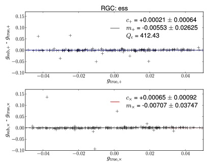
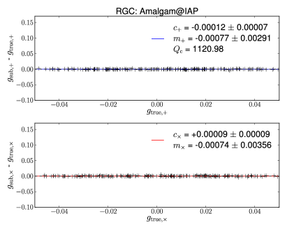
As an example, the top panel of Fig. 14 shows the per-subfield submitted shear from RGC for the “ess” team. The plotted quantities are used to derive $m_{i}$ and $c_{i}$ for the $Q_{\rm c}$ metric. This team has several subfields with highly discrepant submitted shears, well beyond the expected standard deviation of $\lesssim 0.001$ per subfield. This branch is the worst case for this team, which had fewer outliers in CGC.

To explore the effect of outliers, we did a systematic test for outliers in the submitted shears, identifying (for each branch and team) those fields for which the submitted shears were discrepant by more than $|\Delta g|=0.01$ in more than 75 per cent of submissions. In general, these subfields were consistent across methods; that is, if two teams had a certain number of outlier fields in a given branch, they were almost always the same set of subfields. Those subfields were commonly ones with higher values for the PSF defocus (or, for the “ess” team, higher values of trefoil); we defer a more detailed exploration of the impact of defocus on shear systematics to Sec. 5.5. For the “ess” team, the reason for the outliers shown in Fig. 14 is fairly clear: they used a sum of three Gaussian components to describe the PSF, which makes it particularly difficult to model PSFs with defocus or trefoil. In contrast, the middle panel of that figure shows a comparable plot for the Amalgam@IAP team, which modeled the full PSF, and does not show significant outliers. Finally, the bottom panel shows images of the PSF for the eleven subfields in RGC for which the “ess” results were seriously discrepant. As shown, in about three cases the PSF has the characteristic “donut” shape of highly out-of-focus images; such data would likely be eliminated from a shear analysis in a real dataset. These subfields were problematic for several other methods. In other subfields, there is a triangular shape characteristic of trefoil, which seems to have been less problematic for other methods that have a more flexible representation of the PSF.

For those teams and branches for which outlier fields were identified, we recalculated the $m_{i}$, $c_{i}$, and $Q_{\rm c}$ values after excluding the outlier fields. We found that while errors from the linear regression on $m_{i}$ and $c_{i}$ decreased substantially (sometimes tens of percent after excluding only a few percent of the subfields), the changes in $m_{i}$, $c_{i}$, and $Q_{i}$ were in general not coherent. In many cases, results for different submissions from the same team in the same branch would change in different directions. There were three combinations of branch and team with coherent changes in results after excluding outliers (in two cases the results were almost always worse, and in one case they were almost always better).

Several other teams had problems with outliers that were not identified in the previous test. (Identifying them as outliers would require a smaller threshold on $|\Delta g|$ and on the number of times the field has a discrepancy for it to officially be called an outlier.) These include MBI, which (like ess) used a sum of Gaussians to describe the PSF; and MegaLUT. We recalculated the results for these teams after excluding the fields with the 10 per cent worst defocus in CGC. For MBI, the results of excluding the subfields with the worst defocus did have a coherent effect, but with opposite signs in the control and realistic galaxy experiments, increasing $Q_{\rm c}$ in the former by as much as a factor of two and lowering it in the latter by a similar amount. We speculate that the difficulty in modeling these PSFs may not lead to some systematic overall effect because the hierarchical inference of $p(\varepsilon)$ might be partially compensating for imperfect PSF model fits by adjusting the galaxy model fits accordingly. For MegaLUT, the changes in results after excluding the high-defocus subfields were substantially smaller than for MBI.

Due to the generally inconclusive results of excluding outliers, with no team showing a strong trend towards improved overall results, for the rest of this paper we do not exclude outlier fields. However, in in Appendix D we also tabulate the outlier-rejected estimates of $\langle m\rangle$ and $c_{+}$ for the ess, MBI and MegaLUT submissions, these being the teams most affected by outliers.

We note that in future challenges it may be a good idea to permit participants to assign weights to their submitted per-subfield shears, so they can indicate regimes in which their PSF modeling or shear estimation does not work. Our results also suggest that PSF modeling with a low-order decomposition into sums of Gaussians may be inadequate to describe realistic PSFs, and can significantly affect the shear estimates.

5 Overall results

In this section, we present results for the control and realistic galaxy experiments for all teams.

5.1 What results are shown

Figure 15: $Q_{\rm c}$ (top) and $Q_{\rm v}$ (bottom) for constant- and variable-shear branches in the control and realistic galaxy experiments. The errorbars show the possible range of $Q$ values for a submission with shear calibration biases that would nominally give a particular $Q$ value. As shown, the sizes of these ranges depend strongly on $Q$, and are smaller for space than for ground branches.

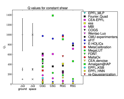
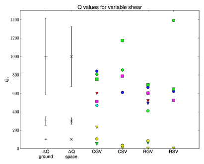
To avoid showing many submissions from each team in each branch, we adopt a fair and consistent way to select a single submission per branch from each team. For the teams discussed in Sec. 4, we have already stated what submissions will be used here. For the remaining teams, the selection was done as follows:

• FDNT: We use FDNT v1.3, with a self-consistent set of resolution and SNR cuts (submissions with names that include “r12_sn15”).

• E-HOLICs: We use their “snfixed200” submission, which have a self-consistent set of noise bias corrections.

• MaltaOx: We use the best results for LensFit with oversampled PSFs and self-calibration included.

• ess: We only use their RGC results, with the priors on $p(\varepsilon)$ derived from the deep fields (submission name “nfit-rgc-06-nfit-flags-02”).

• CMU experimenters: Only one submission per branch.

• CEA_denoise, MetaCalibration, EPFL_MLP / EPFL_MLP_FIT, EPFL_KSB, EPFL_HNN, Wentao Luo: Best submission in each branch.

• GREAT3-EC (or re-Gaussianization): These results used the shear estimation example script described in Appendix B. As noted there, for several reasons the results are not science-quality shear estimates and therefore the results have no reflection on science papers that use this algorithm. However, since it is a stable algorithm in the public domain, and one of the few moments-based methods, we include it in this section to provide a basic point of comparison.

Results for the following teams are not shown in this section: miyatake-test (for reasons described in Sec. 3), BAMPenn, and HSC/LSST-HSM. The BAMPenn results included some bugs that mean the results do not correctly reflect the real performance of the method. The HSC/LSST-HSM submissions used the HSC/LSST software pipeline with the same shear estimation method as in the GREAT3 example scripts purely as a sanity check of the pipeline.

5.2 Basic $Q$ results

Figure 16: Comparison between the $Q_{\rm v}$ predicted from the constant-shear branch results (CGC), and the actual $Q_{\rm v}$ results for variable shear (CGV).

Figure 17: Multiplicative and additive biases for constant-shear branches in the control (left) and realistic galaxy (right) experiments, for ground (top) and space (bottom) branches. For each branch, we show the averaged (over components) multiplicative bias $\langle m\rangle$ vs. $c_{+}$, the additive bias term defined in the coordinate system defined by the PSF anisotropy. The axes are linear within the target region ($|m|<2\times 10^{-3}$ and $|c|<2\times 10^{-4}$, shaded grey) and logarithmic outside that region.

Figure 18: Left and right columns show results for $\langle m\rangle$ (top; averaged over components) and $c_{+}$ (bottom) for ground and space branches, respectively. Each panel compares results for control vs. realistic galaxy experiments. The axes are linear within the target region ($|m|<2\times 10^{-3}$ and $|c|<2\times 10^{-4}$, shaded grey) and logarithmic outside that region. The black dashed line is the 1:1 line.

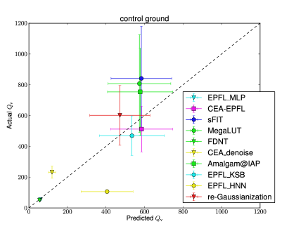
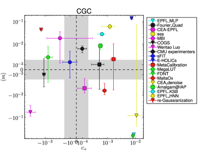
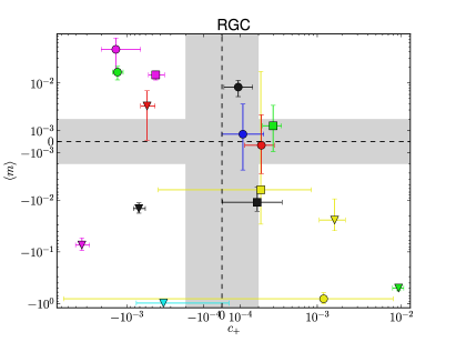
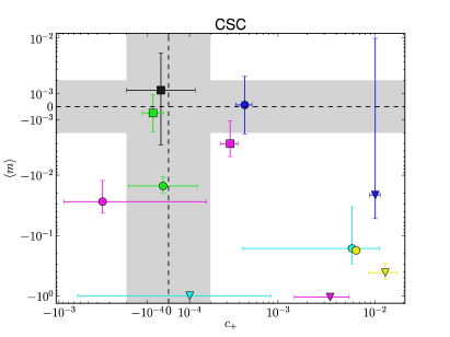
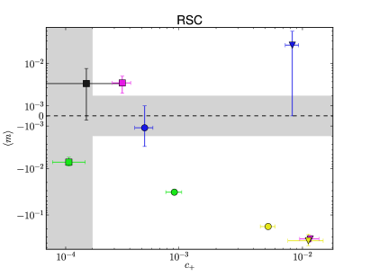
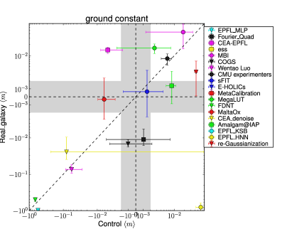
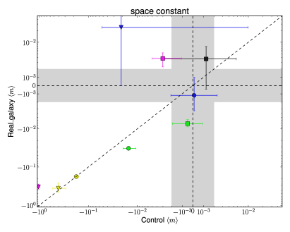
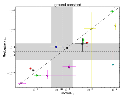
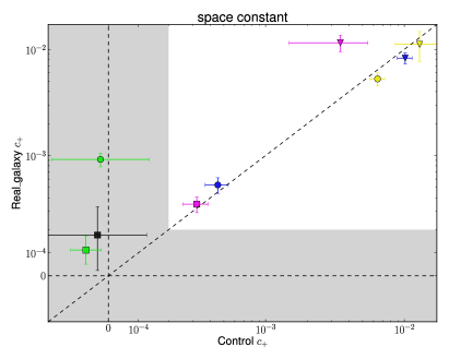
In this subsection, we present the $Q$ results for all teams. Fig. 15 shows $Q_{\rm c}$ and $Q_{\rm v}$ for the control and realistic galaxy experiments.

Several trends from Sec. 4 are evident here. For example, the results for sFIT are quite consistent across all branches shown here. The MegaLUT results are consistently better for variable shear than for constant shear, presumably because of a low-level $m$-type bias, to which $Q_{\rm c}$ is more sensitive than $Q_{\rm v}$. The results for Amalgam@IAP and CEA-EPFL are good in many branches, but exhibit significant fluctuations due to partial cancellations of biases. The results for Fourier_Quad with a realistic weighting scheme are quite good, but degraded compared to the results with the unrealistic weighting schemes.

The errorbars in Fig. 15 show that for lower $Q$ values, the uncertainty in $Q$ is very small. However, near the target $Q$ values, small uncertainties in $m$ and $c$ become large uncertainties in $Q$. These errorbars are quite non-Gaussian, so for example the difference between $Q=500$ and $1000$ for control space branches is significantly more than the $2\sigma$ suggested by the plot. It is apparent that in many branches, 2–3 teams performed well enough that the differences between their $Q$ values (and between the target of $\sim 1000$) are not statistically significant.

One basic question is whether the results in the constant and variable shear branches are consistent. We cannot directly compare $Q_{\rm c}$ and $Q_{\rm v}$, because they respond to systematic errors in different ways. However, for a given constant-shear submission, we can use the recovered $m$ and $c$ values to predict $Q_{\rm v}$ by simulating variable shear submissions with those $m$ and $c$, and then checking their $Q_{\rm v}$. Comparing the predicted $Q_{\rm v}$ with the actual one (for the same experiment and observation type) is a valid consistency check. We show this comparison for CGC and CGV in Fig. 16, with a reasonable level of consistency within the relatively large errors on the $Q_{\rm v}$, and at most a $2\sigma$ discrepancy for one team. The plots for the other experiments and observation types show similar constant vs. variable shear consistency.

5.3 Multiplicative and additive shear biases

This section will focus on Fig. 17, which shows the multiplicative and additive shear biases ($m$ and $c$) for the constant-shear branches in the control and realistic galaxy experiment. All $m$ and $c$ values are also tabulated in Appendix D. Unlike $Q_{\rm c}$, $m$ and $c$ have well-understood errorbars. On these plots, the errorbars are different sizes for different methods. In some cases, it is only an apparent difference (due to the mixed linear and logarithmic axes), but there is some variation in the scatter in shears that we will explore in Sec. 5.6.

Figure 19: Shear biases for CGC, similar to Fig. 17 but using $m_{1}$ and $m_{2}$ (defined using the pixel coordinate system).

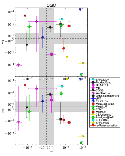
We begin by discussing the top left panel of Fig. 17, which shows $\langle m\rangle$ (averaged over components) vs. $c_{+}$ for CGC. Not surprisingly, the teams that are located near the center of this plot (small $|m|$ and $|c|$) are the ones with high $Q_{\rm c}$ factors for this branch (Fig. 15).

A few methods (COGS, MegaLUT, MetaCalibration) are notable in having multiplicative biases consistent with being in the target region, but highly significant detections of additive bias. Both COGS and MetaCalibration include multiplicative bias corrections, but no additive bias corrections were implemented by the end of the challenge period.

5.3.1 Impact of morphology

Comparing the left and right sides of Fig. 17 would reveal the impact of realistic galaxy morphology. However, to facilitate an easier comparison, Fig. 18 explicitly compares $\langle m\rangle$ (averaged over components) and $c_{+}$ values for control vs. realistic galaxy experiments, with results tabulated in Table 5. For ground-based simulations, the $\langle m\rangle$ comparison is in the top left panel. Many methods are consistent with the 1:1 line, meaning that the calibration bias does not show any detectable impact from realistic galaxy morphology. Moderate differences in model bias due to realistic galaxy morphology can be seen for many teams, with typically a $\sim$ per cent level impact of realistic galaxy morphology on multiplicative calibration biases, although the sign of the change in $\langle m\rangle$ depended on method.

The top right panel of Fig. 18 shows how $\langle m\rangle$ changes from control to realistic galaxy experiment for space-based simulations. Again, some methods exhibit no significant model bias due to realistic galaxy morphology (but note that sFIT included this effect in their simulations, and explicitly calibrated it out), while others have typically $\sim 1$ per cent level calibration changes.

The bottom left panel of Fig. 18 shows $c_{+}$ for CGC vs. RGC, with everything from complete consistency to strong differences in $c_{+}$ in these branches, implying that realistic galaxy morphology can in some cases cause additive biases.

Finally, in the bottom right panel of Fig. 18, the $c_{+}$ are consistent between control and realistic galaxy experiments for space-based simulations for most methods. It seems that for space simulations, removing the PSF anisotropy is similarly difficult for both parametric and realistic galaxy models.

5.3.2 Impact of ground- vs. space-based PSF

Comparing the top and bottom rows of Fig. 17 reveals the effects of using a space-based PSF rather than a ground-based PSF. Note that the numerical values of the $c_{+}$ and $\langle m\rangle$ changes are shown in Table 5. Focusing first on the control experiment (left side), the $c_{+}$ values shifted to the right (more positive) in space data for the majority of the methods. Note that if $c_{+}$ scales linearly with PSF ellipticity (a model that we will validate in Sec. 5.4), then $c_{+}$ for the space branches should be larger than in the ground branches by a factor of $\sim 2$. This may explain the changes in $c_{+}$ for several teams, but not all, implying that in some cases the additive systematics have some additional dependence on the form of the PSF beyond its ellipticity.

Comparing multiplicative biases for CGC and CSC, they are either statistically consistent between space and ground or more negative for space branches; curiously, they did not become more positive for any teams. Given the wide diversity of methods and the apparent lack of commonality between many that exhibit similar behavior between ground and space data, it is difficult to draw conclusions, but the pattern is indeed interesting.

These results were for the control experiment. If we compare RGC vs. RSC (right panels), we see that the differences in $c_{+}$ and $\langle m\rangle$ between space and ground simulations in the realistic galaxy experiment are similar to what was seen for the control experiment for all teams except CEA_denoise. This finding suggests that the effect of the type of PSF (space vs. ground) on additive and multiplicative biases does not typically depend on whether the galaxies have realistic morphology or are simple parametric models.

5.3.3 Use of pixel coordinate system

The top left panel of Fig. 17 shows $m$ vs. $c$ for CGC in the coordinate system defined by the PSF anisotropy, whereas Fig. 19 shows the same in the pixel coordinate system. In a few cases (e.g., CEA-EPFL, Fourier_Quad, and MetaCalibration to some degree though it is noisier), $m_{1}$ and $m_{2}$ have opposite signs, and thus average out to something closer to zero (after rotating to the PSF anisotropy coordinate frame) for $m_{+}$ and $m_{\times}$, resulting in $Q_{\rm mix}<Q_{\rm c}$.

5.4 Understanding the linear model

In this section, we explore the linear model for shear systematics, Eq. (7), by considering some alternative models of shear measurement bias.

It is commonly assumed that the main source of $c$-type biases is leakage from PSF anisotropy into galaxy shear estimates, which should be proportional to the amplitude of the PSF ellipticity. (However, there are physical models that violate this assumption, nor is this assumption completely obvious for all methods.) If the assumption is correct, we can write an alternative model:

$$g^{\rm obs}_{i}-g^{\rm true}_{i}=m_{i}g^{\rm true}_{i}+a_{i}g^{\rm PSF}_{i}$$ (11)

Here, the $a_{i}$ prefactors are average values across an entire galaxy population that likely depend on the distribution of SNR, resolution, morphology, and PSF type. In the coordinate system defined by the PSF anisotropy, $g^{\rm PSF}_{+}=|g^{\rm PSF}|$ and $g^{\rm PSF}_{\times}=0$. We can therefore fit to this new model, and if the additive errors are proportional to the PSF anisotropy, then we should find $c_{+}\propto a_{+}$, where the constant of proportionality is an effective mean $|g^{\rm PSF}|$ for that branch.

Fig. 20 compares $c_{+}$ and $a_{+}$ for CGC (top) and RSC (bottom), though the results are quite similar for CSC and RGC as well. The best-fit line relating $c_{+}$ and $a_{+}$ goes through nearly all the points, indicating that the linear model works well (except for EPFL_HNN) for a wide variety of shear estimation methods. The slopes of the best-fitting lines for CGC, RGC, CSC, and RSC are 0.025, 0.016, 0.039, and 0.037, respectively, corresponding to the effective mean per-branch $|g^{\rm PSF}|$.

$a_{+}$ is essentially the fraction of PSF anisotropy that leaks into galaxy shear estimates. For the methods that have $c_{+}$ within the target region, the $a_{+}$ values indicate that typically $<1$ per cent of the PSF shear contaminates the galaxy shears. Several methods are in the range of 1–10 per cent leakage, and the worst case scenarios involve leakage of tens of per cent. For data with a narrower (wider) range of PSF anisotropies but otherwise similar properties (so that $a_{+}$ is the same), the additive bias $c_{+}$ will be better (worse) than is shown here. (Note that the histogram of PSF shears in GREAT3 is in Appendix A.3.)

In real data, selection biases that correlate with PSF direction also induce additive systematics. While these operate at some level in GREAT3 due to different weights being assigned to galaxies depending on their direction with respect to the PSF, in real data selection biases should be more important given the need to identify galaxies. In that case, this simple linear model may no longer be valid. It seems reasonable that selection biases will cause $c_{+}$ to scale with $|g^{\rm PSF}|$, but it is not obvious that the scaling should be linear.

The success of the simple linear PSF contamination model of Eq. (11) in describing additive bias in GREAT3, evidenced by Fig. 20, is striking. However, we note that the GREAT3 simulations were designed without many effects found in real data that potentially cause additive bias (see Sec. 2.2 for a list) but are not directly related to the PSF. These may cause additive biases to show more complex dependencies in real data.

Another question about the linear model for shear calibration biases is whether these methods have a nonlinear response to shear. This question was already addressed in the STEP2 challenge (Massey et al., 2007a). In that case, the shears were positive in the CCD coordinate system, and the nonlinearity test involved a term proportional to $g_{\rm true}^{2}$. In GREAT3, the per-component shears can be positive or negative, so the simplest low order nonlinear terms are proportional to $g_{\rm true}^{3}$ or ${\rm sign}(g_{\rm true})g_{\rm true}^{2}$. We can think of these as being the next order beyond linear of a series expansion of some unknown function representing the shear response.

We carried out fits with an additional term defined in either of these two ways, and checked for nonzero prefactors for the nonlinear terms. In general, the results for all methods are consistent with zero. When considering constant shear branches in the control and realistic galaxy experiments, there are 81 submissions (across all branches and teams) that we use in this section, and therefore 162 fits when we use both shear components. Regardless of which form we use for the nonlinear term, its prefactor differs from zero at $>2\sigma$ for nine of the 162 fits, or 5.6 per cent, which is consistent with what we expect if no methods have nonlinear response. Moreover, these $>2\sigma$ deviations are not consistently found in any particular team, but are for a range of teams. We conclude that the GREAT3 results show no sign of a nonlinear shear response for any method. However, with a maximum value of $|g_{\rm true}|\leq 0.05$, we are not very sensitive to nonlinear shear response, and studies that go into the cluster shear regime may need to redo this test.

Figure 20: For CGC (top) and RSC (bottom), we compare the additive bias $c_{+}$ in the standard linear bias model, Eq. (7), against $a_{+}$ for the alternative model in Eq. (11). $a_{+}$ is a constant of proportionality relating additive shear systematics to the PSF ellipticity. The axes are linear for $|a_{+}|<2\times 10^{-3}$ and $|c_{+}|<2\times 10^{-4}$ (where the latter is our target region for additive systematics, shown in grey) and logarithmic outside that region; we use vertical lines to indicate the linear-logarithmic boundary in $a_{+}$. The best-fit slope relating $c_{+}$ and $a_{+}$ is shown as a dashed magenta line. It only appears curved because we show combined log and linear axes with an unequal aspect ratio.

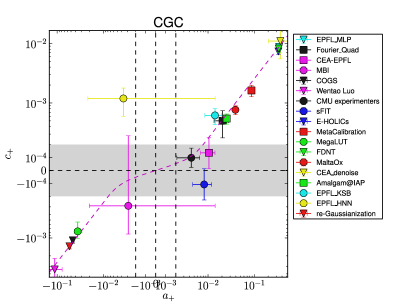
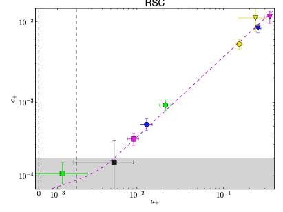
5.5 Dependence of results on detailed PSF properties

In this section, we check how results for each method depend on the PSF properties within the branch. Note that the PSF properties in the control and realistic galaxy experiments are discussed and shown in Appendix A.3 and Fig. 27.

For this test, we split the subfields within a branch into those with atmospheric PSF FWHM, defocus, or $|g^{\text{PSF}}|$ above and below the median values. Then we refit the submitted shears for those subsets to estimate $m_{i}$ and $c_{i}$ values. We can compare the $m_{i}$ and $c_{i}$ for those with better vs. worse values of seeing, defocus, and PSF shear, and compare with the overall $m_{i}$ and $c_{i}$ for the branch.

5.5.1 Atmospheric PSF FWHM

We begin in CGC, splitting into samples with better or worse atmospheric PSF FWHM (seeing). The results are in Fig. 21, in which the top panel compares the $\langle m\rangle$ values for the better and worse seeing half of the subfields (with numerical values tabulated in Table 6).

Figure 21: For CGC, we show how $\langle m\rangle$ (top) and $c_{+}$ (bottom) change when we split the subfields in the branch into 50 per cent above and below the median atmospheric PSF FWHM. The axes are linear within the target regions for $m$ and $c$, and logarithmic outside them, with the target regions shaded in grey. The thick blue arrows point towards the direction of reducing shear systematics, i.e., towards the center. In all panels, any points that represent a significant change in the plotted quantity for better or worse seeing subfields also have an arrow showing how the results have changed compared to using the whole field. The legend gives the $Q_{\rm c}$ value for the original submission from each team.

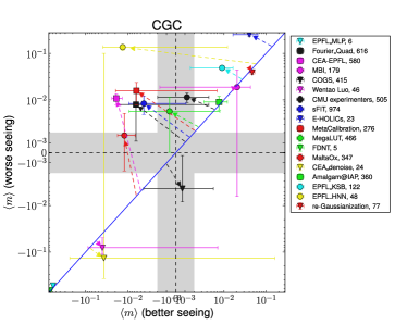
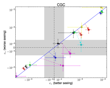
The teams for which $\langle m\rangle$ differs for better vs. worse seeing have a more negative (positive) calibration bias for better (worse) seeing.

The bottom panel of Fig. 21 shows that many teams have consistent $c_{+}$ for better and worse seeing, with the rest having a more strongly positive $c_{+}$ for the better seeing subfields. The worse $c_{+}$ values for better seeing subfields may come from the fact that the optical PSF (which is often more elongated than the atmospheric component) dominates. Indeed, the correlation coefficient between PSF FWHM and $|g^{\rm PSF}|$ in CGC (RGC) is -0.23 (-0.25), with a significance of $p=0.001$ ($3\times 10^{-4}$). Thus, the worse seeing subfields have a consistently rounder PSF, which can reduce additive systematics.

The results for both the $\langle m\rangle$ and $c_{+}$ trends were similar in RGC to what we have shown here for CGC, which is a point that we will revisit in some of our later tests.

5.5.2 Defocus

In Fig. 22, we show how $c_{+}$ in CGC changes when we split at the median absolute value of defocus (with results tabulated in Table 6). The results for many methods exhibit a more strongly nonzero $c_{+}$ for stronger defocus. It is not surprising that additive systematic errors are worse when out of focus, because defocus amplifies the effect of other aberrations like coma and astigmatism on the PSF (Schechter & Levinson, 2011), giving a noticably more elliptical PSF. Appendix A.3 shows that we allowed a relatively wide range of defocus values in the ground branches, which explains why its effects are noticeable despite the fact that the atmospheric PSF is normally thought of as being dominant.

The multiplicative biases $m_{+}$ and $m_{\times}$ (not shown) do not typically change when splitting by defocus, except for sFIT and MetaCalibration, with smaller changes for MBI and Amalgam@IAP. For MBI, the representation of the PSF as the sum of three Gaussians may be the limiting factor in describing out-of-focus PSFs. For sFIT, the problem may arise from the use of simple PSFs (rather than a range of complex PSF with varying defocus) for the simulations used to calibrate the shears. Explicitly deriving calibrations for different PSFs may ameliorate this problem. A similar issue is likely at play for MetaCalibration, which derived an average shear response using all subfields, rather than one for each PSF. It is unclear why the calibration changes with defocus for Amalgam@IAP, but it may be because of difficulties in finding a well-defined maximum likelihood for many galaxies in the more strongly defocused cases.

Figure 22: For CGC, we compare additive biases $c_{+}$ when splitting the subfields into those with defocus above or below the median. The axes are linear within the target region (shaded grey), and logarithmic outside them. The thick blue arrows point in the direction of reduced shear systematics. Any points that represent a significant change compared to results for the entire branch have an arrow showing that change, as well.

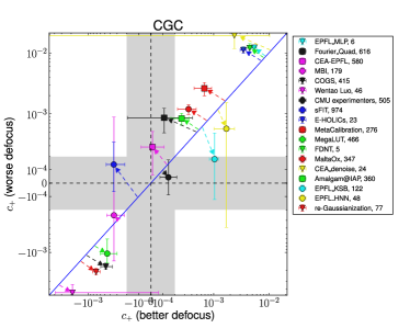
In space simulations (CSC), splitting by defocus had qualitatively similar effects on shear systematics as for CGC. However, the shifts are smaller in magnitude for space simulations, likely because the range of defocus is much smaller for space simulations than for ground ones (see App. A.3).

Our findings are similar in the realistic galaxy experiment, suggesting that the dependence of shear systematics on defocus is independent of realistic galaxy morphology.

5.5.3 PSF ellipticity

When splitting the subfields by $|g_{\rm PSF}|$, the results are consistent with those of Sec. 5.4, where additive systematics were shown to scale linearly with the PSF ellipticity.

5.6 Effective noise level of estimated shears

Here we explore the effective noise level of the estimated shears. In principle, galaxy shapes were arranged in a way that cancels out shape noise, so that the dominant source of error in the estimated shears is measurement error due to pixel noise. However, the shape noise cancellation is imperfect at low $S/N$, so that the submitted shears include some shape noise as well. Fig. 23 shows the per-galaxy and per-component scatter ($\sigma_{g}$) in the estimated shears for CGC, estimated from fitting the model of Eq. (7) and finding the scatter in the shear estimates for the subfields (then dividing by $\sqrt{10^{4}}$ to get a per-galaxy value). This scatter thus includes both the measurement error and any residual shape noise due to noise in the weights, which can be seen as an additional manifestation of susceptibility to pixel noise. There is a weak relationship between $\sigma_{g}$ and $Q_{\rm c}$, with all methods that have $Q_{\rm c}\gtrsim 300$ having $0.1\lesssim\sigma_{g}\lesssim 0.25$. Methods with lower $Q_{\rm c}$ scores have higher scatter by as much as a factor of 40; the exceptions to this rule are re-Gaussianization and EPFL_KSB, which notably are fairly simple moments-based methods. In a few cases, outliers are an issue, but even with $5\sigma$ clipping, the trend at low $Q_{\rm c}$ is quite evident. This figure for RGC looks very similar. For the space simulations, the effective per-galaxy $S/N$ was slightly higher, reducing the $\sigma_{g}$ values slightly, the overall trend is the same.

The straightforward interpretation of these results is that for methods with $Q_{\rm c}\gtrsim 300$, the per-object measurement error is typically subdominant to shape noise, whereas some methods with lower $Q_{\rm c}$ allow significant leakage of pixel noise into the estimated shears.

Figure 23: Scatter in the estimated shears (per galaxy and per component) vs. $Q_{\rm c}$ for each method in CGC. The horizontal line indicates a typical level of shape noise in realistic galaxy samples.

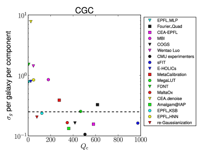
5.7 Catalog-level tests

For several teams, we carried out catalog-level tests that involve using subsets of the galaxies. For example, we split the galaxies into subsamples with $S/N$ above and below the median; and likewise for resolution factor defined as in Hirata & Seljak (2003) using the adaptive second moments, and Sérsic index $n$. These splits use the true (not estimated) values of these parameters, to preserve shape noise cancellation. The methods used for this test are CEA-EPFL, MegaLUT, Fourier_Quad, re-Gaussianization, and sFIT, which include a range of shear estimation methods. For Fourier_Quad, we re-estimated ensemble shears for the galaxy subsets as in Eq. (22).

In general, biases such as noise bias depend on both the flux-based $S/N$ and the resolution. Thus, a split by a single galaxy property may not isolate a particular bias. Instead, these splits are a way to estimate how much the shear systematics might change for a particular method when dividing the galaxy sample in a way that changes the mean $S/N$, resolution, or Sérsic $n$.

Fig. 24 shows the results for $\langle m\rangle$ (left) and $c_{+}$ (right) after dividing the galaxy sample in CGC in these three ways. In each case, we plot the results for subsamples against each other, so a method that is robust to changes in these quantities would be on the $1:1$ line. Methods that are not on that line must by definition move either to the upper left or lower right. We consider each method in turn.

The $\langle m\rangle$ and $c_{+}$ results for CEA-EPFL show only a mild dependence on $S/N$, but a much greater dependence on resolution and on Sérsic n. MegaLUT has less statistically significant trends, with the most clear ones being the change $\langle m\rangle$ with $S/N$ and the change in $c_{+}$ with Sérsic $n$. The multiplicative bias $\langle m\rangle$ for Fourier_Quad is quite robust to splitting by any of the three parameters, but $c_{+}$ shows significant changes for $S/N$ splits, with the change for Sérsic $n$ being less significant. re-Gaussianization exhibits significant dependence on all of $S/N$, resolution, and Sérsic $n$, qualitatively consistent with the findings in Mandelbaum et al. (2012), but little change in $c_{+}$. Finally, for sFIT, both $\langle m\rangle$ and $c_{+}$ change when splitting by all three parameters, though the changes with $S/N$ are marginal in significance. Given that this team explicitly derived calibration factors to remove additive and multiplicative biases from the entire population (not as a function of galaxy properties), these trends are not surprising. There is no reason to expect the calibration factors to be valid for subsamples. This exercise merely emphasizes the necessity of rederiving them when using subsamples, or even changing weighting schemes.

If we check in RGC whether the changes in these methods are consistent across control and realistic galaxy experiments, then we cannot do the comparison for sFIT due to a lack of catalogs for that submission. However, of the remaining methods used, only the re-Gaussianization results when splitting the galaxy sample are the same in CGC and RGC, which is interesting given the significant model bias due to realistic galaxy morphology seen for this method in Sec. 5.3. The results for CEA-EPFL when splitting by resolution and Sérsic $n$ are the same in RGC as in CGC, but the change in $\langle m\rangle$ when splitting by $S/N$ has the opposite sign as in CGC. The MegaLUT method shows much stronger trends in both $\langle m\rangle$ and $c_{+}$ in RGC when splitting by all three parameters than in CGC. Finally, for Fourier_Quad, the sign of the $c_{+}$ changes when splitting by resolution and Sérsic $n$ is reversed in RGC compared to CGC.

In CSC, we can check how the use of space simulations changes the results when dividing the galaxy sample (for all but re-Gaussianization, which only has results on ground branches). The CEA-EPFL and sFIT team results show different signs and/or magnitudes of changes in shear systematics when splitting by galaxy properties in CSC vs. in CGC. For MegaLUT, the value of $c_{+}$ changes when splitting by $S/N$ and resolution more significantly in CSC than in CGC. For Fourier_Quad the difference in $c_{+}$ between subsamples in resolution and Sérsic $n$ changes in sign in CSC compared to CGC. These findings suggest that essentially all teams considered here have trends in shear systematics with galaxy properties that are different in space vs. in ground data.

Figure 24: For CGC, we compare the $\langle m\rangle$ (left) and $c_{+}$ (right) values that we get by splitting the galaxies at the median value of $S/N$ (top), resolution (middle), and Sérsic $n$. The legend indicates the team and the $Q_{\rm c}$ value for the original submission using all galaxies. Arrows on each plot are shown for those teams for which the results for the subsamples differ from the overall results by more than 10 per cent, and are drawn from the overall value to the results for the subsamples.

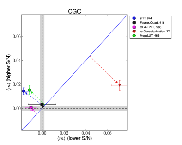
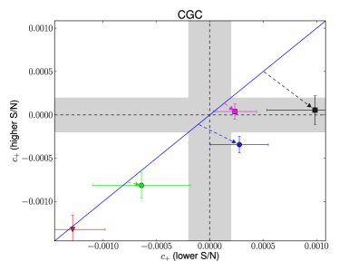
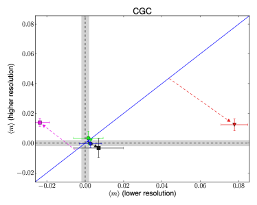
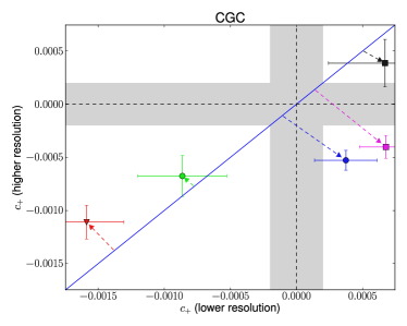
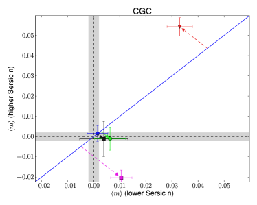
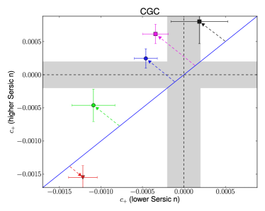
5.8 Comparison with GREAT08 and GREAT10 results

In this section we compare quantitatively with the results from GREAT08 (Bridle et al., 2010) and the GREAT10 galaxy challenge (Kitching et al., 2012), to the limited extent that is possible given the different challenge designs and the lack of error analysis in previous challenge results.

For GREAT08, the fairest comparison is between GREAT3 CGC and GREAT08 RealNoise_Blind bulge $+$ disk galaxy results. We cannot compare $Q$ values since they are defined in a different way, so instead we compare $\langle m\rangle$ and $c_{+}$, bearing in mind that even this comparison is complicated by the broader, more realistic distributions of galaxy properties in GREAT3. In the left column, middle row of figure C3 in Bridle et al. (2010), the number of methods that have $|\langle m\rangle|<0.05$, $0.02$, and $0.005$ is $7$, $2$, and $0$. In GREAT3, these numbers are 12, 10, and 6, using only the fair comparison sample results used throughout Sec. 5 rather than the best submission per team for this branch. We are also ignoring the uncertainty on these $\langle m\rangle$ values for consistency with how we did the calculation for GREAT08 given its lack of error estimates. The upper left panel of figure C4 (b$+$d) in Bridle et al. (2010) suggests that $8$ ($4$) methods have $|c_{+}|<1\times 10^{-3}$ ($2\times 10^{-4}$), whereas in GREAT3 CGC these numbers are 9 (3). The latter comparison is particularly complicated by different choices for the PSF ellipticity distribution in these challenges, since we showed in Sec. 5.4 that for essentially all methods, $c_{+}$ is linearly proportional to PSF ellipticity.

For GREAT10, the simplest comparison is with the inferred $m$ and $c$ values in table 3 of Kitching et al. (2012), again ignoring noise due to the fact that no uncertainties are quoted. However, two of the better-performing submissions in that table have no $m$ or $c$ estimates, since they used a power spectrum analysis. In the absence of more information we will include them in the best category that we consider, $|\langle m\rangle|<0.005$ and $c_{+}<2\times 10^{-4}$. Given this choice, the number of methods in GREAT10 with $|\langle m\rangle|<0.05$, $0.02$, and $0.005$ is $7$, $5$, and $2$, which should again be compared with 12, 10, and 6 in GREAT3. All 12 methods in table 3 of Kitching et al. (2012) had $c$ values within $2\times 10^{-4}$, with the range of PSF ellipticities being different from that in GREAT3, but not to a very large extent.

The GREAT3 results show that significant progress has been made in controlling multiplicative biases since GREAT08 and GREAT10, with the situation for additive biases being less clear. However, additive biases are easier to identify in real data (for example, using star-galaxy cross-correlations), so this situation fairly reflects the community’s focus on the more pernicious multiplicative biases. Given that, as discussed in Appendix A.4, the GREAT3 simulations have a realistic $S/N$ distribution with an effective cutoff of $12$, this improvement in control of multiplicative biases is a significant achievement reflecting tremendous progress in the weak lensing community as a whole.

6 Lessons learned about shear estimation

In this section, we discuss lessons learned about shear estimation based on the analyses in Sections 4 and 5. Our focus is on results that are more general than just a single method; conclusions for individual methods can be drawn from earlier plots and discussion.

6.1 What do we learn about shear estimation in general?

Many teams that participated in GREAT3 used model-fitting methods, which must make choices about which pixels to use for the fitting. The results in Sec. 4.1 highlight the importance of truncation bias due to use of overly-small modeling windows. Truncation bias can potentially be several per cent (multiplicative bias), and also is a source of additive bias; its magnitude makes it relevant for present-day surveys, and could potentially be worse in the case of blends (which might lead to the choice of a more restricted modeling window). These model-fitting methods make choices about which models to use, with two popular options being a single Sérsic model (Amalgam@IAP, sFIT, MBI) and a sum of a bulge and disk Sérsic models with fixed $n$ (COGS, gfit). The good performance of these methods suggests that use of Sérsic profiles can reduce model bias that is observed with, e.g., shapelets or other models that do not describe galaxy light profiles as well as Sérsic profiles.

Several methods of calibration were successful for model-fitting methods: external simulations for which the inputs were iteratively updated until the output galaxy properties match those in the GREAT3 data (sFIT), derivation of calibration corrections from a deep subset of the same data (COGS), and addition of a penalty term to the $\chi^{2}$ to reduce noise bias (Amalgam@IAP). External simulations are always limited by their realism, though use of iterative methods seems to be helpful. Calibration corrections from deep data do not, in principle, require external validation. Addition of a penalty term to the $\chi^{2}$ does require external simulations to check that the penalty term really removes the noise bias.

Our results in Sec. 5.4 confirm the applicability of the linear model for shear calibration biases in the $|g|\lesssim 0.05$ regime for all methods that participated in GREAT3. Several methods showed tendencies for multiplicative biases defined in the pixel coordinate system to differ between the component along the pixel axes and along their diagonals, similar to what was seen in e.g. Massey et al. (2007a). In all cases, the additive biases $c_{+}$ were linearly proportional to the amplitude of the PSF ellipticity (of order 0.1 per cent of the PSF ellipticity for the best methods, and more typically 1–5 per cent). It is possible that some biases in real surveys but not GREAT3 would violate this pattern (e.g., selection biases that depend on the PSF anisotropy).

The results for many methods show a dependence on PSF properties like the FWHM, defocus, and ellipticity. In some cases, the results seem to have been calibrated to work on average, so that they are worse for better or worse quality data than for the challenge overall. Defocus tends to result primarily in additive (not multiplicative) systematics. Some methods are particularly sensitive to outliers in defocus, which results in more complicated-looking PSFs; it is difficult to assess to what extent that sensitivity is intrinsic to the PSF correction method (because those PSFs violate one of its assumptions) vs. arising from how the PSFs are modeled (because of limitations of the PSF modeling software). Some future surveys will have additional diagnostic data regarding PSFs; these results suggest that it may be helpful to incorporate this information in the PSF modeling and shear estimation process.

When splitting galaxy samples by $S/N$, resolution, or Sérsic $n$, we observe statistically significant trends for the five methods that were considered; these trends are sensitive to real galaxy morphology (control vs. realistic galaxy experiment) and the type of data (space vs. ground). In contrast, the variation in shear systematic errors due to data properties like atmospheric PSF FWHM or defocus was fairly robust to realistic galaxy morphology.

Comparing ground vs. space data, additive systematics seem to be more important for the latter. In space branches, several teams saw their $c_{+}$ become significantly more positive, which contributed towards there being almost entirely positive $c_{+}$ submissions in space branches. However, not all the teams with negative $c_{+}$ in the ground branches submitted to the space branches.

Finally, the effective noise level of the shear estimates (measurement error due to pixel noise) showed a weak inverse relationship with $Q$. For the majority of the methods (especially those with $Q_{\rm c}\gtrsim 200$), the values of $\sigma_{g}$ per component were fairly consistent across methods. This confirms the general tendency to select shear estimation methods based on their multiplicative and additive biases, rather than separately considering their measurement errors.

6.2 The impact of realistic galaxy morphology

Many methods, including some that performed extremely well, show a small but statistically significant change in model bias due to realistic galaxy morphology, with order of magnitude 1 per cent. Realistic galaxy morphology can also result in additive systematics. Our findings for the order of magnitude of this effect for multiple methods is consistent with the finding for the im3shape software (Kacprzak et al., 2014). For some methods, realistic galaxy morphology was more important for space branches than for ground (e.g., the sFIT team had to explicitly calibrate out the bias due to realistic galaxy morphology only for space).

One key limitation in lessons learned about realistic galaxy morphology in GREAT3 is that, since its impact is relatively small (typically detected at $\sim 3\sigma$), it is hard to distinguish between space and ground results or clearly identify trends with other data properties. However, this in itself is good news for future surveys, since it provides an indication that model bias due to realistic galaxy morphology may rank behind other effects, such as noise bias, in terms of its direct impact on shear measurements.

In real data with a substantially deeper source population than is represented in the sample of galaxies from COSMOS used as the basis for the GREAT3 simulations, these results will have to be revisited due to the larger fraction of irregular galaxies at higher redshift (e.g., Bundy, Ellis & Conselice, 2005).

7 Conclusions

We have presented results for the control and realistic galaxy experiments of the GREAT3 challenge, the goal of which was to test ensemble shear estimation given a galaxy population with a realistic distribution of size, $S/N$, ellipticity, and morphology, and with a (known) fairly complicated PSF. A key result is that, within the ability of the simulations to determine systematics at this level and bearing in mind that some effects are not included in them, a range of methods can now carry out shear estimation with systematics errors around the level required by Stage IV dark energy surveys.

We have explored how the results for each team depend on the galaxy and PSF properties; and explored the impact of realistic galaxy morphology by comparing the control and realistic galaxy branches. Our conclusions on these points are summarized in Sec. 6, with the main one being that shear systematic errors due to realistic galaxy morphology are, for those methods for which we have a clear detection, typically of order $\sim 1$ per cent. While significant enough that future surveys must take these effects into account, this source of model bias error is subdominant when compared to the level of noise bias expected for similar galaxy populations to those in GREAT3 (e.g., Kacprzak et al., 2012; Melchior & Viola, 2012; Refregier et al., 2012). In Paper II, we will use the other branches of the challenge to explore whether these overall results from Sec. 6 carry over to the case where the PSF is not known.

Treating the participants as a fair subset of the community, it seems that model-fitting methods now dominate the field in both popularity and (broadly) performance. Some differences between methods may relate to implementation details rather than true issues with a method. Unlike a decade ago, moments methods are now a minority. However there are some highly interesting alternative methods, for which we have seen the introduction and/or evident maturity in GREAT3 (some based on Bernstein & Armstrong (2014); MetaCalibration; self-calibration for LensFit as carried out by the MaltaOx team; hierarchical inference as done by the MBI team; machine learning based methods like MegaLUT; and Fourier_Quad), adding variety and quality to the field. This includes the introduction of some teams that just infer ensemble shears (MBI, BAMPenn, ess, Fourier_Quad) rather than per-object shears; however, a demonstration of these methods on variable shear data will be crucial for their more general acceptance.

Choices related to calibration of shears were quite varied, with some teams that aim for an unbiased measurement (e.g. BAMPenn, ess, MBI) and others that apply calibrations in a variety of ways. Aside from external simulation-based calibrations, which are subject to the limitation that the calibrations are only as good as the simulations, a few more sophisticated options were tried. These include iterative external simulations that get updated until the outputs match those in the dataset that is being analyzed (sFIT), analysis of a deep subset of the same data (COGS), and self-calibration using manipulations of the images themselves (MaltaOx, MetaCalibration). These alternatives appear promising, and avoid some of the objections to the most basic brute-force calibration. The utility of the deeper data to several teams, either for calibrations or deriving galaxy property distributions, suggests that future surveys may find it useful to have a deeper subsurvey, as indeed many already intend to do. Several teams used self-calibration methods (MetaCalibration and MaltaOx) and hierarchical-inference (MBI) methods that in principle could be used to remove the biases in many other shear estimation methods. These newer methods were not among the very top performers, but did impressively well for new implementations, so it will be interesting to follow their future development.

We also have a number of conclusions about GREAT-type challenges based on the GREAT3 challenge process. Unfortunately, the variable shear simulations were less powerful than originally intended at detecting systematic biases in the shear fields. Despite our best efforts in attempting to define a metric with a reasonably small variance, $Q_{\rm v}$ was noisier than $Q_{\rm c}$, the constant-shear metric. However, for the methods that submitted results to constant and variable shear branches, the results were consistent with the estimated shears having the same underlying biases (within the errors), as we would expect. Future challenges that want to determine biases with variable shear fields may require substantially larger data volumes than in GREAT3. Future challenges may also want to allow participants to assign weights to downweight data that they do not want to use, rather than requiring shear estimates for all fields.

After the end of the challenge, we found that use of a metric based on systematics in the coordinate system defined by the PSF anisotropy resulted in accidental preference for methods with calibration biases in the coordinate system defined by the pixel frame that were related as $m_{1}\approx-m_{2}$. While this had little effect on the challenge itself, it highlights the fact that a challenge with a public leaderboard including $Q$ values (even without any multiplicative and additive biases) cannot be considered truly blind. Participants sometimes made choices based on feedback from the leaderboard, which at times was useful in helping them avoid completely futile pathways, but at times may have involved tuning to low levels of noise rather than making real conclusions. Thus, if the goal is a truly blind challenge (which helps evaluate existing methods rather than assisting the development of new ones), then we recommend that future challenges consider some change in the public leaderboard. For example, the public leaderboard could use a subset of the data, with the real leaderboard that uses all the data being released only after the end of the challenge. An alternative would be to tell participants a range in which their $Q$ values fall (e.g., $0<Q<200$, $200<Q<400$, and so on). Both options would give participants a basic idea of their results (allowing them to check, e.g., shear conventions and avoid submitting junk by accident) while not encouraging them to potentially tune to the noise.

A final point for future challenges and even planning for future surveys relates to the importance of the $S/N$ definition. It is quite common to use galaxies above some $S/N$ limit, but in GREAT3, we found that depending on the $S/N$ definition, the effective $S/N$ can vary by nearly a factor of two. For example, as stated in the handbook, we initially set a $S/N>20$ limit to ensure that most teams would be able to compute shears for all galaxies, with shape noise effectively canceled. The disadvantage of this limit was that we would not dig too deeply into the noise bias-dominated regime. However, we found in practice (see Appendix A.4) that our $S/N$ estimator was so optimal as to be completely unachievable in practice, given that it assumes perfect knowledge of the light profile. Our tests showed that the lower $S/N$ limit using more practical estimators is around $12$. On the positive side, this meant that the results have a more realistic level of noise bias, but on the negative side, it meant that the simulations were less powerful in constraining shear systematics. This finding highlights the importance of how $S/N$ is defined both for future challenges and for parameter forecasts and mission specifications for future lensing surveys.

In conclusion, GREAT3 has led to substantial progress in quantifying shear systematics for a wide range of methods, including traditionally recognized effects like noise and model bias due to mismatch between assumed and real galaxy light profiles in the control branch, but also newer effects like truncation bias and model bias due to realistic morphology, the latter of which was enabled by the use of HST data for the simulations. The results show that the field has made significant advances in the years since the end of the GREAT10 challenge, particularly in controlling multiplicative biases, and that community challenges can be beneficial by inspiring the creation or development of new shear estimation methods. Within this field, there are both new and established methods that are now capable of handling weak lensing data from upcoming Stage III surveys, provided adequate care is taken over identified sources of bias. Although development will be needed in many areas, the GREAT3 results provide new reasons to be optimistic about delivering reliably accurate shear estimates at Stage IV survey accuracy.

Appendix A GREAT3 challenge details

In this appendix, we summarize some details of the GREAT3 challenge that were not included in the handbook.

A.1 Galaxy intrinsic ellipticity distribution

The galaxy intrinsic ellipticity distribution, or $p(\varepsilon)$, is important, since many methods make assumptions about or try to infer it. We measure this distribution for the GREAT3 galaxy samples using parametric fits to COSMOS galaxies.

The galaxy selection in each subfield has three goals: first, it should roughly preserve the joint size, $S/N$, morphology, and ellipticity distributions of real galaxy samples; second, each subfield should have a similar $S/N$ cutoff (which depends on the PSF as well as the pixel noise); and finally, the galaxies should be sufficiently resolved that essentially all methods can measure them. In ground branches, where the PSF size varies substantially from subfield to subfield, it is not obvious that the galaxy population will have the same $p(\varepsilon)$ in each subfield after these cuts.

In Fig. 25, we show the $p(\varepsilon)$ for several subfields in CGC and CSC, with several apparent trends.

Figure 25: The intrinsic ellipticity distribution $p(\varepsilon)$ for CGC (top) and CSC (bottom), for three subfields. For CGC, the legend shows the subfield index and atmospheric PSF FWHM. Both panels show intrinsic ellipticity distributions for disk and bulge galaxies from Miller et al. (2013).

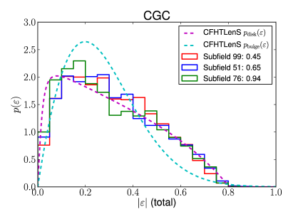
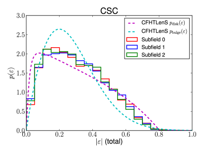
First, the $p(\varepsilon)$ are similar for space and ground branches. Second, within different subfields in CSC, there are small fluctuations in the $p(\varepsilon)$, but these appear consistent with noise. For ground branches, the PSF FWHM results in quite different populations being represented in each subfield. For this figure, we deliberately show one subfield with atmospheric PSF FWHM around the median, along with the subfields with the minimum and maximum values of PSF FWHM. Thus, we have maximized population differences due to our FWHM-dependent galaxy selection process. However, $\langle\varepsilon\rangle$ is only slightly smaller in the worst seeing subfield than for the more typical and best subfields, and part of the difference here is due to statistical fluctuations. The results are similar for the realistic galaxy experiment, and for variable shear branches. Thus, the $p(\varepsilon)$ are largely stable within and across branches. Moreover, they are reasonably consistent with a linear combination of observationally-motivated distributions for bulges and disks derived in a completely different way and used in Miller et al. (2013), as shown on the plot.

The resolution cut is slightly ellipticity-dependent for the smallest galaxies, as shown in Fig. 26 (the 2D distribution of half-light radius and ellipticity). In general, $\lesssim 5$ per cent of the galaxies are small enough to be affected by this problem. Also, this effect is irrelevant in space branches, where the cuts remove very few galaxies.

Figure 26: The 2D histogram of galaxy half-light radius $r_{1/2}$ and ellipticity magnitude $|\varepsilon|$ for subfield 51 in CGC, which has atmospheric PSF FWHM around the median value.

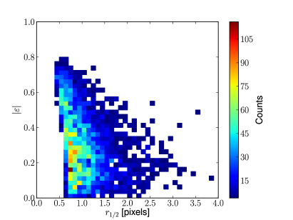
A.2 Lensing shears

Here we describe the distributions from which the lensing shears were drawn.

In constant-shear branches, the lensing shears had random orientations, with magnitudes between $0.01\leq|g|\leq 0.05$. The distribution of magnitudes within this range is $p(|g|)\propto|g|$, which emphasizes higher shear values and thus increases our sensitivity to systematic errors in the shear.

In variable shear branches, each galaxy had an applied shear and magnification according to a shear power spectrum. The shear power spectrum came from interpolation between tabulated ones for a particular cosmological model with three median redshifts $z_{\text{med}}=0.75$, $1.0$, and $1.25$. However, the power spectrum was altered in two ways. First, the amplitude was doubled, to increase our sensitivity to multiplicative biases. Second, to make the power spectrum one that cannot be guessed by participants, we added a term corresponding to a sum of shapelets with randomly chosen amplitudes (of order 10 per cent of the original power spectrum amplitude). For more details, see the publicly available simulation scripts on the GREAT3 GitHub page.

A.3 Atmospheric and optical PSF properties

While the handbook contained details on many inputs to the PSF models, here we show the outputs that are relevant for tests carried out in this paper, especially in Sec. 5.5.

Fig. 27 shows the distributions of the seeing (atmospheric PSF FWHM) in two branches; the defocus for ground and space-based simulations; and finally the effective PSF ellipticities including all components. As shown (top left), the seeing distributions in CGC and RGC are consistent, modulo small noise fluctuations. This consistency is important for the comparison between control and realistic galaxy experiments, since consistency in PSF properties leads to consistency in the simulated galaxy populations.

The top right panel of Fig. 27 shows the distribution of defocus values for the optical PSF in the ground-based simulations. CGC and RGC are again consistent, with most subfields have a maximum defocus of $1/2$ wave, but with a tail to higher values. The subfields that seemed most problematic in Sec. 4.8 are those with higher defocus values, which suggests that identifying and removing such data could be advantageous. The bottom left panel shows the defocus distribution for simulated space-based data, and as expected, the simulated distribution is roughly a factor of ten narrower than for ground data. Moreover, CSC and RSC are consistent, which facilitates comparison between control and realistic galaxy experiments.

Finally, Fig. 27 (bottom right) shows the distributions of effective PSF shear for four branches. Typically this quantity is $\lesssim 0.05$, consistent with real data; two-sided KS tests show that the PSF shears are consistent between pairs of branches that are meant to represent the same data type (e.g., CSC and RSC, CGC and RGC).

Figure 27: Distributions of PSF properties across all subfields in various branches. Top: Seeing (left) and defocus distributions (right) for CGC and RGC. Bottom left: Defocus distributions for CSC and RSC; note the smaller dynamic range compared to the ground branches. Bottom right: Distribution of PSF shear in the four constant-shear branches in the control and realistic galaxy experiments.

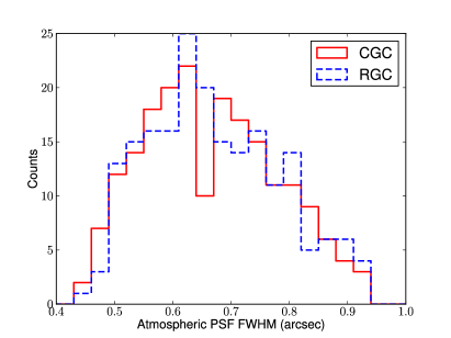
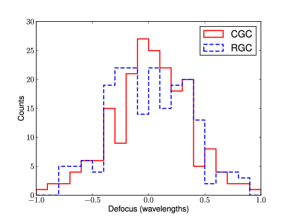
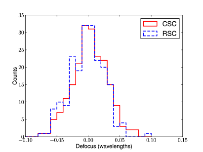
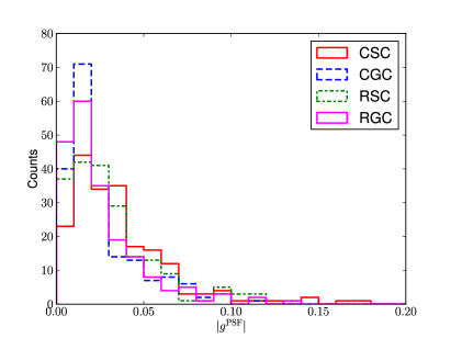
In both ground and space simulations, there is a positive correlation between the absolute value of defocus and $g^{\rm PSF}$, $\sim 0.33$ in both cases (with a $p$-value of order $10^{-7}$).

A.4 Galaxy $S/N$ distributions

The galaxy $S/N$ distribution in the GREAT3 simulations is important because it determines the level of noise bias, an important systematic error for shear estimation. The handbook states that the galaxies have $S/N\geq 20$, which is higher than the cutoff that is used by many methods in real data. However, the $S/N$ estimator used to impose that cutoff is an optimal one that assumes perfect knowledge of the galaxy profile (which is unachievable in real data). Thus, to relate the quoted $S/N$ cutoff to what is used in real data, we must use a more realistic $S/N$ estimator.

For this purpose, we considered two $S/N$ estimators. One is the $S/N$ within an elliptical Gaussian aperture determined using the best-fitting elliptical Gaussian model for the PSF-convolved galaxy. Another is the ratio of sextractor outputs FLUX_AUTO$/$FLUXERR_AUTO. Fig. 28 shows $S/N$ distributions using the second definition for several subfields in ground (top) and space (bottom) branches.

Figure 28: The distribution of galaxy $S/N$ using the second $S/N$ estimator described in the text, for three subfields in CGC (top) and CSC (bottom).

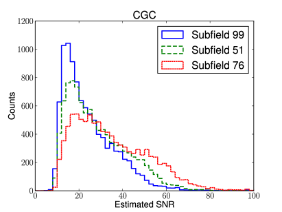
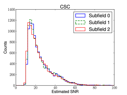
As shown, the $S/N$ distribution is quite uniform across subfields in space branches. The 5th percentile for $S/N$ is $\sim 12$. In contrast, the $S/N$ distribution for ground branches varies with the subfield; the ones shown here are the same as in Fig. 25, with maximal variation in the atmospheric PSF FWHM. Subfields with worse seeing typically have higher average galaxy $S/N$. The 5th percentile $S/N$ value is 11.3, 12.0, and 13.5 for subfields with the best, median, and worst atmospheric PSF FWHM. If we use the elliptical Gaussian-based $S/N$ estimate, then the plots shift slightly to the right (higher $S/N$), with a lower limit of $\sim 14$ instead of 12 for space branches. This is still a far cry from the nominal $S/N>20$ limit using the optimal estimator, which highlights the need for care in comparing predictions with different estimators.

Appendix B Example scripts

The GREAT3 Executive Committee distributed a shear estimation example script (called simple_shear.py) on the GREAT3 GitHub page. This example script estimates per-galaxy shears for all galaxies and outputs them as catalogs in the format expected by the publicly available presubmission scripts. Teams could take this code to do the bookkeeping while substituting their per-galaxy shear estimation routine in place of the one in the example script.

The example script uses the GalSim (Rowe et al., 2014) implementation of the re-Gaussianization (Hirata & Seljak, 2003) PSF correction method; see those papers for more details of the algorithm and implementation. Because the script is a simple and fast example (not meant to get a science-quality shear estimate), it applies only a simply-derived calibration correction that does not include all known systematics. For the “shear responsivity” (Bernstein & Jarvis, 2002) describing how galaxies with a particular distortion respond to a lensing shear, the script uses an overly-simplistic expression rather than a more accurate one (both available in the above reference). It also uses a simple but inaccurate way of estimating the RMS distortion of the galaxy population, rather than more accurated but more complicated methods that are available in the literature (e.g., Reyes et al., 2012) as an input to the responsivity calculation. Finally, the default settings for initial guess of object size lead to convergence to a local minimum for the space branches that cuts out the outer parts of the PSF, resulting in very wrong shear estimates (but accurate centroid estimates). Fine-tuning the initial guesses is necessary for this script to give reasonable results on space simulations.

Appendix C Shear estimation methods

C.1 Amalgam@IAP

C.1.1 PSF modelling

The PSF modeling was performed using the PSFEx package (Bertin, 2011) to compute the PSF model for the star postage stamps. The PSF modeling procedure starts by normalising and re-centering point-source images to a common “PSF grid” using a regular image resampling technique. The coefficients of a set of basis functions of point-source coordinates $X_{c}(\boldsymbol{\theta})$ (simple polynomials) are adjusted in the $\chi^{2}$ sense to every PSF “pixel” to compute a coarse PSF model and its spatial variation, in the form of a set of tabulated PSF components $\boldsymbol{\phi}_{c}$.

The model is further refined by adding corrections $\Delta\boldsymbol{\phi}_{c}$ by minimising the following cost function over all pixels $i\in{\cal D}_{s}$ from all point sources $s$:

$$\begin{split}E(\Delta\boldsymbol{\phi}_{1,2,...})&=\\ &\!\!\!\!\!\!\!\!\sum_{s}\sum_{i\in{\cal D}_{s}}\frac{\left(p_{i}-f_{s}\sum_{c}X_{c}(\boldsymbol{\theta})\left[\phi_{c\,i}^{\prime}(\boldsymbol{x}_{s})+\Delta\phi_{c\,i}^{\prime}(\boldsymbol{x}_{s})\right]\right)^{2}}{\sigma_{i}^{2}}\\ &+\sum_{c}\frac{\|\Delta\boldsymbol{\phi}_{c}\|^{2}}{\sigma_{\phi}^{2}},\end{split}$$ (12)

where $p_{i}$ is the value of pixel $i$, with uncertainty $\sigma_{i}$, and $f_{s}$ the flux of point source $s$. $\sigma_{\phi}$ sets the amplitude of the regularisation term. In practice, $\sigma_{\phi}\approx 10^{-2}$ represents a good compromise between fidelity and robustness of the solution.

The prime indicates a resampled version of the PSF components; e.g., the value of pixel $i$ with coordinates $\boldsymbol{x}_{i}$ in the image of PSF $\boldsymbol{\phi}$ resampled at the point-source position $\boldsymbol{x}_{s}$ with PSF sampling step $\eta$:

$$\phi_{i}^{\prime}(\boldsymbol{x}_{s})=\sum_{j}h_{s}\left(\boldsymbol{x}_{j}-\eta(\boldsymbol{x}_{i}-\boldsymbol{x}_{s})\right)\phi_{j},$$

where $h_{s}(\boldsymbol{x})$ is the interpolation function.

The version of PSFEx used for the GREAT3 challenge is identical to v3.17.1 except for the interpolation function, which is either a Lanczos-4 or Lanczos-5 kernel instead of the default Lanczos-3. Support for measurement vectors as PSF dependency parameters (PSFVAR_KEYS) was added early in the challenge to allow PSFEx to map PSF variations as a function of any set of columns in an ASCII list, through SExtractor’s ASSOC mechanism.

The PSFEx configuration used for GREAT3 differs from the default one in a few minor ways. The first difference is in the use of super-resolution, adopting a constant sampling step $\eta$ of 0.6 image pixels for all branches. This sampling step offers the best compromise between robustness and accuracy given the limited number of PSF images for branches with a constant PSF. Also, the full star postage stamp size is used for each branch. PSF variations are modelled using 0th and 5th degree polynomials of star coordinates for constant and variable PSF branches, respectively. Finally, the noise on point source images is assumed to be purely additive, setting PSF_ACCURACY to 0.

C.1.2 Galaxy shape measurement

Galaxy shapes are measured using SExtractor v2.19.15 (Bertin & Arnouts, 1996; Bertin, 2011). The measurement process involves independently fitting each galaxy image with a Sérsic model convolved with the local PSF model from PSFEx. To avoid galaxy detection problems, the Amalgam@IAP team used a detection image to explicitly tell SExtractor about the gridded galaxy positions.

The vector of Sérsic model parameters $\boldsymbol{\theta}$ includes the $(x,y)$ centroid position, amplitude, effective radius, aspect ratio, position angle and Sérsic index. Physically meaningful constraints (e.g., amplitude $>0$) are imposed on all parameters except position angle through a change of variables $\boldsymbol{\theta}\rightarrow\boldsymbol{\theta}^{\prime}$. For instance, for the aspect ratio (parameter $\theta_{\rm aspect}$) the Amalgam@IAP team instead constrain the transformed parameter $\theta_{\rm aspect}^{\prime}$ defined as

$$\theta_{\rm aspect}^{\prime}=\ln\frac{\ln\theta_{\rm aspect}-\ln 0.01}{\ln 100-\ln\theta_{\rm aspect}}.$$ (13)

Individual ellipticities from the aspect ratio and position angle of the best-fitting galaxy model are used directly. SExtractor also extracts the associated uncertainties and their correlation coefficient from the covariance matrix of the fitted parameters.

The fit itself is achieved by minimising a quadratic cost function with the Levenberg-Marquardt algorithm using the LevMar library. The cost function is the weighted sum of squared residuals plus a quadratic penalty term

$$E(\boldsymbol{\theta})=\chi^{2}(\boldsymbol{\theta}^{\prime})+\sum_{i}\frac{(\theta_{i}^{\prime}-\mu_{\theta_{i}})^{2}}{\sigma^{2}_{\theta_{i}}}.$$ (14)

where the sum is over galaxy model parameters $i$. The version of SExtractor used by default has $\sigma_{\theta_{i}}\equiv\infty$ for all parameters (no penalty).

The fitting process typically converges in 50-100 iterations. Compared to the latest publicly available version of the package, the following changes were made to the SExtractor code for GREAT3:

• Fitting area (normally set automatically) is limited to the size of the GREAT3 galaxy images to avoid overlapping with neighbouring galaxies.

• Sampling of the model is forced to 0.3 image pixel, instead of the default which depends on the input PSF model.

• The step used in difference approximation to the Jacobian in LevMar is set to $10^{-4}$.

• Penalty parameters for the aspect ratio are set to $\mu_{\theta_{\rm aspect}}=0$ and $\sigma_{\theta_{\rm aspect}}=1$ to disfavour very large ellipticities for the most poorly resolved objects, without significantly affecting the results for more resolved galaxies.

• The default, modified $\chi^{2}$ (which is more robust for partially overlapping objects) is replaced with a regular $\chi^{2}$.

Finally, the SExtractor configuration used by the Amalgam@IAP team reflects the details of the GREAT3 simulations: the background is set to 0 ADU; the GAIN is set to 0 (equivalent to infinite); and the MASK_TYPE detection masking parameter is usually NONE.

C.1.3 Galaxy weighting

The Amalgam@IAP team used a modified inverse-variance weighting scheme based on the full covariance matrix from SExtractor (approximated by the Hessian calculated by the LevMar minimization engine) to account for possible covariance between parameters and for differences in the recovery of $e_{1}$ and $e_{2}$ components. This covariance matrix forms the basis for the per-galaxy shear covariance matrix. To avoid giving too much weight to high $S/N$ objects, the Amalgam@IAP team added a constant $\sigma_{s}^{2}$ to the diagonal entries. For constant-shear branches, they used the full per-object covariance $\mn@boldsymbol{C}_{i}$ to estimate the shear as

$$\hat{\gamma}=\left(\sum_{k}C^{-1}_{k}\right)^{-1}\sum_{j}C^{-1}_{j}\boldsymbol{e_{j}},$$

using the 2-vector $\boldsymbol{e_{j}}$ and $2\times 2$ matrix $\mn@boldsymbol{C}^{-1}$. In practice, the difference between using the full covariance matrix and its isotropic approximation was small.

For variable shear branches, the Amalgam@IAP team used the provided corr2 code with isotropized scalar weights defined as

$$w_{i}=\frac{2}{\sigma_{i,1}^{2}+\sigma_{i,2}^{2}+2\sigma_{s}^{2}},$$

where the denominator represents the quadrature sum of measurement error and shape noise.

C.2 BAMPenn

This team used the Bayesian Fourier Domain (BFD) method from Bernstein & Armstrong (2014), which relies on weighted moments calculated in Fourier space and a prior for the noiseless distribution of galaxy moments (e.g., from deep data). Weighting is implicit rather than explicit in this Bayesian calculation. The ensemble shear from the mean of the Bayesian posterior should be unbiased in the limit that many galaxies are used for shear estimation, potentially avoiding noise biases that can plague maximum-likelihood methods. It does not result in a per-object shear estimate.

The submissions made during the challenge period came from an immature software pipeline and had errors that were identified after the fact. Currently, the machinery is in place only for a constant-shear analysis, not variable shear.

C.3 EPFL_gfit

All submissions by the EPFL_gfit team used the gfit method. A few submissions also used a wavelet-based DWTWiener denoising code from Nurbaeva et al. (2011), integrated into gfit. The gfit method uses a maximum-likelihood, forward model-fitting algorithm to measure galaxy shapes. An earlier version of gfit, used in the GREAT10 galaxy challenge (Kitching et al., 2010, 2012), was described in Gentile, Courbin & Meylan (2012). The version used in GREAT3 is completely new, written in Python and relies on the NumPy, SciPy and PyFits libraries. The software has a modular design, so that additional galaxy models and minimizers can be plugged in fairly easily. The behavior of gfit is controlled though configuration files.

gfit requires catalogs generated via an automated process from input galaxy and PSF mosaic images by SExtractor (Bertin & Arnouts, 1996). The following galaxy models, for which images are generated using GalSim, are currently supported:

1. A pure disk Sérsic model.

2. A sum of an exponential Sérsic profile (Sérsic $n=1$) to model the disk and a de Vaucouleurs Sérsic profile ($n=4$) to model the bulge. The disk and bulge share the same centroid and ellipticity.

3. A model similar to the previous but with a varying disk Sérsic index.

Almost all GREAT3 submissions used the second galaxy model, with the following eight parameters: galaxy centroid, total flux, flux fraction of the disk, bulge and disk radii, and ellipticity.

Fitting can be performed with two minimizers, using input SExtractor catalogs to get initial guesses for galaxy centroids, fluxes and sizes. The first minimizer is the SciPy Levenberg-Marquardt non-linear least-squares implementation. The second is a simple coordinate descent minimizer (SCDM), a loose implementation of the Coordinate Descent algorithm. In the SCDM, the model parameters are sequentially varied in a cycle, to explore all directions in parameter space. After each cycle, the change in the objective function is measured and the sense of variation maintained or reversed. The step size for each parameter is dynamically adjusted based on previous iterations. The algorithm is, by nature, slow but quite robust, with a failure rate below 1/1000 on GREAT3 images. Several stopping conditions are available and can be combined.

The EPFL_gfit submissions used a simple weighting scheme that was one of the options used by CEA-EPFL (below), involving constant weighting for all galaxies except those that have unusually large fit residuals, which are rejected entirely (typically $<1$ per cent of the galaxies).

C.4 CEA-EPFL

The CEA-EPFL team used an object-oriented framework written in Python and usable in other contexts than GREAT3 with minimal changes, including:

• Galaxy shape measurement (gfit from Sec. C.3).

• Weight calculation (sfilter).

• PSF estimation (star shape measurement, PSF interpolation, PCA decomposition and reconstruction).

• Image coaddition routines.

• Wavelet-based tools for deconvolution, denoising, coaddition, and super-resolution.

gfit was described in Sec. C.3, but the remaining pipeline elements used in GREAT3 are described below.

C.4.1 Weighting scheme

The sfilter tool uses catalogs produced by gfit to assign a weight to each galaxy.

In GREAT3, two weighting schemes were used. The simpler scheme involved eliminating entries with large fit residuals by giving them weights of zero. The more complex scheme involved assigning weights based on PCA analysis of the RMS between ellipticities fitted by gfit on GREAT3 data and those obtained after running gfit on GREAT3-like simulated data. The galaxy simulations were created using GalSim with GREAT3-like PSF, noise and $S/N$; the galaxy parameters were motivated by the outputs from a gfit analysis of the RSV branch. A PCA decomposition was then performed on a vector with first component $|\Delta e|=\sqrt{(e_{1,\text{out}}-e_{1,\text{in}})^{2}+(e_{2,\text{out}}-e_{2,\text{in}})^{2}}$. The other PCA components were either (a) flux, disk and bulge radii, disk fraction, gfit output parameters or (b) SExtractor FWHM, size, $S/N$, flux, and gfit disk and bulge radii.

The first component, $|\Delta e|$, was plotted against various PCA components to select a cut-off value $v_{0}$ that separated regions of low and high $|\Delta e|$. A weight $w_{\text{low}}$ was assigned to all galaxies with $v<v_{0}$, with $w_{\text{low}}=0.6$ for choice (b), and $w_{\text{low}}=0.2$ for choice (a).

C.4.2 PSF estimation

For the three experiments with constant PSFs that were provided for the participants, the CEA-EPFL team used the provided PSFs directly. The spredict tool was used to estimate the PSF at the positions of galaxies in the variable PSF and full experiments. The version of spredict used in GREAT3 supports two PSF models:

• An elliptical Moffat profile, based on maximum-likelihood fitting using GalSim to generate images. This was used in a few submissions to the ground branches.

• A data-driven model based on PCA decomposition of selected PSF images (with sufficiently high $S/N$, either $>20$ or $>30$) into either 10, 15, or 20 PCA components.

More details of these algorithms will appear in Paper II.

C.4.3 Differences between GREAT3 submissions

The differences between submissions in a given branch arose mainly from the size of the postage stamps used for the fits; constraints placed on galaxy model parameters; minimizer options; weight functions; choice of galaxy models (though most used the second one in Sec. C.3); and occasionally attempts to include wavelet-based denoising.

C.5 CEA_denoise

The CEA_denoise team denoised the GREAT3 galaxy images using a publicly available, multi-scale wavelet-based code mr_filter, based on Starck, Pires & Réfrégier (2006). They then measured unweighted second moments of the denoised galaxy images and noiseless PSF images using SExtractor. Finally, they corrected for PSF convolution by subtracting the PSF moments from the galaxy moments, as proposed by Rhodes, Refregier & Groth (2000) and Melchior et al. (2011).

The CEA_denoise team varied the denoising options (such as using 2 vs. 3 wavelet scales), and selected the denoising methods by comparing the original and filtered galaxies by eye. Strong denoising often resulted in blurry galaxies with correlated noise features around the galaxies.

No weighting was applied to the measured shears.

C.6 CMU_experimenters

The stacking method used by CMU_experimenters was a simple modification of the example script described in App. B. The basic steps were galaxy registration, stacking, and PSF correction of the stacked image.

First, CMU_experimenters measured the weighted first moments (centroids) for all galaxy images. They used the default GalSim interpolation routines to shift each galaxy so the centroid would be at the exact center of the postage stamp. Next, they stacked all $10^{4}$ galaxies in a single GREAT3 image using a simple unweighted average. Finally they used GalSim routines for PSF correction (re-Gaussianization) to estimate the PSF-corrected distortion $\hat{e}$. The shear estimate for the field is simply $\hat{g}=\hat{e}/2$, since the stacked object is effectively round in the absence of a shear. There is a calibration factor of 1.02 for the intrinsic limitations of re-Gaussianization (Mandelbaum et al., 2012).

C.7 COGS

All submissions from the COGS team used the im3shape galaxy model fitting code described in Zuntz et al. (2013).

C.7.1 Galaxy model fitting

The COGS team used a two component galaxy model, with a de Vaucouleurs bulge (Sérsic $n=4$) and an exponential disk ($n=1$). The two components were constrained to have the same half-light radius, centroid, and ellipticity. The seven free parameters in the fit were therefore total flux, bulge-to-total flux ratio, radius, centroid ($x,y$), and ellipticity.

The best-fitting model was identified by minimizing the squared residual between data and model image, using the LevMar implementation of the Levenberg-Marquardt algorithm (see Zuntz et al. 2013 for details). The parameter settings and optimizer termination criteria are given in the im3shape initialization file used for GREAT3. The full galaxy postage stamps were used for all fits.

One important parameter for im3shape is the upsampling, the internal super-resolution at which profiles are drawn and FFT convolutions performed. For speed, early submissions used the native resolution, which causes artifacts in the modeling and increases biases. Later COGS submissions set upsampling = 7. These submissions required similarly upsampled PSF images, which were generated via bicubic interpolation across the noise free PSF images provided with the GREAT3 data. These entries with upsampling = 7 can be considered to be the baseline set of COGS submissions with high precision input settings. These submissions are referenced by their label u7 in this paper.

C.7.2 Noise bias calibration

Some im3shape submissions include a multiplicative calibration factor to correct for expected noise biases in Maximum-Likelihood shape estimation. These can be grouped under the following three labels:

• c1: A correction for an isotropic multiplicative bias $\langle m\rangle=0.0230$ is applied. This expected noise bias was estimated in simulations performed by Kacprzak et al. (2014, table 2) using a galaxy population that differs somewhat from that in GREAT3.

• c2: A correction for an isotropic multiplicative bias $\langle m\rangle=0.0330$ is applied. This bias was estimated using the CGV deep data. The ellipticity of galaxies in the CGV deep fields was measured using im3shape (with upsampling = 7). These images were then degraded by adding noise to match the regular (non-deep) GREAT3 images, and re-measuring the ellipticities. By fitting a polynomial including a constant, linear, and cubic term to $\varepsilon_{1,\text{deep}}$ vs. $\varepsilon_{1,\text{degraded}}$, the COGS team estimated a calibration factor $m(\varepsilon)$ and then calculated an expected calibration bias of $\langle m\rangle=0.033$ based on $p(\varepsilon_{\text{deep}})$. The CGV deep data was used since it exhibited less variation in the image properties than the deep CGC data. This possibly relates to the relatively strong seeing variation identified in the deep CGC data, discussed in Appendix C.20.

• c3: A correction for an isotropic multiplicative bias $\langle m\rangle=0.02943$ is applied. This factor was estimated using the CGV deep data in a similar manner to c2, but using only galaxy models with best-fitting $|\varepsilon_{\rm deep}|<0.9$ in the deep data to estimate $m(\varepsilon)$. This removal of outliers was found to provide a better fit to the (most numerous) galaxies with lower ellipticity values.

No calibration was made for additive biases due to noise, although these are expected where PSFs are anisotropic (Kacprzak et al., 2012).

C.7.3 Differences between GREAT3 submissions

The main differences between submissions were the correction of bugs in the interface between im3shape and the GREAT3 data format, the upsampling, and noise bias calibrations applied. Early submissions used low accuracy settings for rapid basic validation of the GREAT3 data, and are unsuitable as a basis for careful scientific analysis.

However the later set of submissions (with labels u7, c1, c2, and c3 as described above) can be used for fair scientific comparison, and to explore systematic errors in the im3shape approach more generally. All galaxies were given uniform statistical weights when generating submissions.

C.8 E-HOLICS

The E-HOLICs method (Okura & Futamase, 2011, 2012, 2013) is a moment-based method based on the KSB method (Kaiser, Squires & Broadhurst, 1995). One important improvement of the E-HOLICs method compared to KSB is its use of an elliptical (not circular) weight function.

In the E-HOLICs analysis of GREAT3 data, all galaxies that were used for the analysis were uniformly weighted. However, galaxies with estimated ellipticities $>1$ were rejected (i.e., given zero weight). The E-HOLICs team applied a correction for systematic error due to pixel noise as derived in the above references, with different submissions having different corrections.

C.9 EPFL_HNN

The EPFL_HNN method deconvolves the data by the given PSF, represented by linear algebra formalism as a Toeplitz matrix. This allows for solution of the convolution equation by applying the Hopfield Neural Network (HNN) forward recurrent algorithm. At each iteration, the selected neurons of the network (image pixels) are updated to minimize the energy function. To measure the ellipticity of galaxies in deconvolved images, the second order moments of the image autocorrelation function are used (Nurbaeva et al., 2014).

HNN is an unsupervised neural network, so input galaxy stamps could be initialized to zero. To reduce CPU time, the observed data was used as input. The output consists of reconstructed images of the deconvolved galaxies, their autocorrelation functions, and an ellipticity catalog. All galaxies received equal weighting when calculating the average shears, and no calibration correction was applied.

Differences between submissions in each branch include:

• the size of the effective galaxy postage stamp size;

• the pixel updating value (a smaller number gives finer reconstruction, while increasing the iteration number and CPU time); and

• filtering (removing the galaxies for which the HNN algorithm failed to converge).

C.10 EPFL_KSB

The EPFL_KSB team used an implementation of the KSB method (Kaiser, Squires & Broadhurst, 1995; Luppino & Kaiser, 1997; Hoekstra et al., 1998) based on the KSBf90 pipeline (Heymans et al., 2006). The KSB method parametrises galaxies and stars according to their weighted quadrupole moments. In the standard KSB method, a Gaussian filter of scale length $r_{g}$ is used, where $r_{g}$ is galaxy size. The EPFL_KSB team also tried other weighting functions.

The main assumption of the KSB method is that the PSF can be described as a small but highly anisotropic distortion convolved with a large circularly symmetric function. With that assumption, the shear can be recovered to first-order from the observed ellipticity of each galaxy via

$$\gamma=P_{\gamma}^{-1}\left(e^{\rm obs}-\frac{P^{\rm sm}}{P^{\rm sm*}}e^{*}\right),$$ (15)

where asterisks indicate quantities that should be measured from the PSF model at that galaxy position, $P^{\rm sm}$ is the smear polarisability (see Heymans et al. 2006 for definitions) and $P_{\gamma}$ is the correction to the shear polarisability that includes the smearing with the isotropic component of the PSF. The ellipticities are constructed from weighted quadrupole moments, and the other quantities involve higher order moments. All definitions are taken from Luppino & Kaiser (1997). The shear contribution from each galaxy is weighted according to the quadrature sum of shape noise and measurement error, calculated as in appendix A of Hoekstra, Franx & Kuijken (2000).

Submissions from this team fall into two categories: those using the standard KSB Gaussian filter, and those using a combination of KSBf90 and a multiresolution wiener filter with bspline wavelet transform (mr_filter, Starck, Pires & Réfrégier, 2006). The latter submissions tended to perform better. Among the first type of submissions, the better-performing ones use a polynomial fitting formula for $P_{\gamma}$ based on the galaxy size and $S/N$, and rejection of galaxies with extremely large values of $P_{\gamma}$.

C.11 EPFL_MLP

The EPFL_MLP team’s method involved training a Multilayer Perceptron (MLP) Neural Network to measure galaxy shapes. The MLP is a feedforward neural network with one hidden layer (Haykin, 2009; Rojas, 1996). The arctangent function is used as an activation function. The input data are the set of neurons, represented by the galaxy image pixels. The output is the ellipticity catalog. The MLP is trained on simulated data with the standard back-propagation algorithm.

MLP works in two passes. During the forward pass, the weight matrix is applied to the training set, the output is compared to the desired result to obtain the error gradient and to average them over the batch set. During the backward pass, the weight updates $\Delta w$ are calculated from the gradient descent method using the learning rate.

This method uses a batch learning scheme, where the input data is a batch of galaxy stamps and the weights are updated based on the error rate averaged over the batch.

For each submission, the EPFL_MLP team varied the following parameters: the number of neurons in the hidden level, the learning rate, the epoch number (an epoch corresponds to one forward pass and a backward pass), the batch number (batch learning improves stability by averaging), the momentum rate ($\mu$ indicates the relative importance of the previous weight change on the new weight increment).

The training set consists of galaxy images, simulated using GalSim with the following parameters: disk and bulge half-light radii, ellipticity modulus $|e|$, orientation angle, galaxy total flux, bulge ratio, and signal-to-noise ratio.

Both bulge and disk have the same centroid and ellipticity. No weighting was applied to shear estimators, and no calibration factors were applied.

C.12 FDNT

This team used an implementation of the Fourier-domain nulling technique (FDNT, Bernstein 2010). This method estimates a per-galaxy shear in the Fourier domain after PSF effects have been removed by Fourier division (equivalent to deconvolution in real space). This team’s approach was to then apply bias corrections based on image simulations. The bias is a function of (1) $S/N$, (2) resolution, (3) PSF shape, (4) radial flux distribution of the galaxy, and (5) radial flux distribution of the PSF. Additive bias was found to be directly proportional to the PSF shape.

In some cases, galaxies were weighted according to the combination of shape noise (determined from the deep data) and shape measurement uncertainty. All FDNT submissions (v0.1 through v1.3) have the wrong bias corrections applied, and hence all results submitted during the challenge period are not indicative of the real performance of this method once this error is corrected.

C.13 Fourier_Quad

This team used Fourier-space methods described in a sequence of papers (Zhang, 2008, 2010; Zhang & Komatsu, 2011; Zhang, 2011; Zhang, Luo & Foucaud, 2013). The shear estimators for the two components of the reduced shear $g_{1}$ and $g_{2}$ are defined based on the Fourier transform of the galaxy image. There are three quantities: $G_{1}$, $G_{2}$, and $N$, based on multipole moments of the spectral density distribution of the galaxy image in Fourier space:

$$G_{1} = -\frac{1}{2}\int\mathrm{d}^{2}\mathbf{k}\,(k_{x}^{2}-k_{y}^{2})T(\mathbf{k})M(\mathbf{k})$$ (16)

$$G_{2} = -\int\mathrm{d}^{2}\mathbf{k}\,k_{x}k_{y}T(\mathbf{k})M(\mathbf{k})$$

$$N = \int\mathrm{d}^{2}\mathbf{k}\,\left[k^{2}-\frac{\beta^{2}}{2}k^{4}\right]T(\mathbf{k})M(\mathbf{k})$$

where

$$T(\mathbf{k}) = \left|\tilde{W}_{\beta}(\mathbf{k})\right|^{2}/\left|\tilde{W}_{\text{PSF}}(\mathbf{k})\right|^{2}$$ (17)

$$M(\mathbf{k}) = \left|\tilde{f}^{S}(\mathbf{k})\right|^{2}-\left|\tilde{f}^{B}(\mathbf{k})\right|^{2}$$

and $\tilde{f}^{S}(\mathbf{k})$, $\tilde{f}^{B}(\mathbf{k})$, $\tilde{W}_{\text{PSF}}(\mathbf{k})$, and $\tilde{W}_{\beta}(\mathbf{k})$ are the Fourier transforms of the galaxy image, an image of background noise, the PSF image, and an isotropic Gaussian function of scale radius $\beta$, respectively. The latter is defined as

$$W_{\beta}(\mathbf{x})=\frac{1}{2\pi\beta^{2}}\exp\left(-\frac{\left|\mathbf{x}\right|^{2}}{2\beta^{2}}\right).$$ (18)

The factor $T(\mathbf{k})$ is used to convert the form of the PSF to an isotropic Gaussian function. The value of $\beta$ should be at least slightly larger than the original PSF $W_{\text{PSF}}$ to avoid singularities in the conversion. If the intrinsic galaxy images are statistically isotropic, the ensemble averages of the shear estimators defined above recover the shear to second order in accuracy, i.e.,

$$\frac{\left\langle G_{j}\right\rangle}{\left\langle N\right\rangle}=g_{j}+O(g_{1,2}^{3})$$ (19)

for $j=1,2$. Note that ensemble averages are taken for $G_{1}$, $G_{2}$, and $N$ separately; these should be weighted averages, as we will discuss in Sec. C.13.1. In practice, $G_{1}$, $G_{2}$, and $N$ are calculated using discrete Fourier transforms.

In the presence of source Poisson noise, the method is modified/extended by adding more terms into the shear estimators to keep them unbiased. Statistically, the Poisson noise has a scale-independent spectral density in Fourier space. Its amplitude can be estimated at the large wave-number limit, at which the source spectrum is subdominant due to filtering by the PSF. The estimated Poisson noise spectrum can then be subtracted from the spectral density of the image on all scales. This operation is particularly suitable for these shear estimators, as the ensemble averages are taken directly on the spectral density. Finally, the same procedure should be repeated in the neighboring image of background noise, as the Poisson noise in the source image is partly due to the background photons. Removing the source Poisson noise effect requires modification of the definition of $M(\mathbf{k})$ in Eq. (C.13) to

$$M(\mathbf{k})=\left|\tilde{f}^{S}(\mathbf{k})\right|^{2}-F^{S}-\left|\tilde{f}^{B}(\mathbf{k})\right|^{2}+F^{B}$$ (20)

with

$$F^{S,B}=\frac{\sum_{|\mathbf{k}_{j}|>k_{c}}\left|\tilde{f}^{S,B}(\mathbf{k}_{j})\right|^{2}}{\sum_{|\mathbf{k}_{j}|>k_{c}}1}$$ (21)

where $k_{c}$ is a value at which the Poisson noise amplitude dominates over the source signal, typically $\sim 3/4$ of the Nyquist wavenumber.

C.13.1 GREAT3 Experience

In GREAT3, the PSF for constant-shear branches was determined by stacking the spectral densities of the nine provided PSF images. Several different weighting schemes were used, for each of which the weight is a function of the total source flux $F$ (rather than the shape parameters) to avoid introducing systematic biases. Shear estimation for the $j$th component was carried out via

$$\frac{\sum_{i}G_{j,i}W_{i}}{\sum_{i}N_{i}W_{i}}=g_{j}.$$ (22)

Since the background noise in GREAT3 images is uncorrelated, its power spectrum in Fourier space is scale-independent. Thus, its contamination can be directly removed using the source image itself, without using a neighboring background image, rewriting Eq. (20) as

$$M(\mathbf{k})=\left|\tilde{f}^{S}(\mathbf{k})\right|^{2}-F^{S}.$$ (23)

Three weighting options were tried:

1. $W=1$, for which the contribution to the shear signal scales as $(S/N)^{2}$, guaranteeing equal weights for the galaxies in each 90^∘ rotated pair and maximizing shape noise cancellation. However, in terms of contribution to the ensemble shear signal, the bright galaxy pairs are much more important than the faint ones.

2. $W=(S/N)^{-2}$ for galaxies that can be easily identified as 90^∘ rotated pairs by sorting the galaxy luminosity distribution. For two galaxies in a pair, their average flux is used for calculating $W$. For galaxy pairs that are too faint to be identified, $W=(S_{min}/N)^{-2}$, where $S_{min}$ is the minimum galaxy flux from the identified pairs.

3. $W=(S/N)^{-2}$ for all galaxies without identifying pairs.

The first two weighting options are effective in GREAT3 due to its shape noise cancellation, which is not relevant for real data. The last weighting scheme is applicable to real data, though it is not yet optimal.

To calculate the shear-shear correlation function using the shear estimator defined in Eq. (16), the Fourier_Quad team would ideally use (Zhang & Komatsu, 2011)

$$\langle\gamma_{j}(\mathbf{x})\gamma_{j}(\mathbf{x}+\Delta\mathbf{x})\rangle=\frac{\sum_{i}G_{j}(\mathbf{x}_{i})G_{j}(\mathbf{x}_{i}+\Delta\mathbf{x})}{\sum_{i}N(\mathbf{x}_{i})N(\mathbf{x}_{i}+\Delta\mathbf{x})}$$ (24)

The above formula is similar (but not equivalent) to the usual shear-shear correlation calculation using ellipticities $\varepsilon_{1,2}$ and weights $W$:

$$\langle\gamma_{j}(\mathbf{x})\gamma_{j}(\mathbf{x}+\Delta\mathbf{x})\rangle=\\ \frac{\sum_{i}\varepsilon_{1}(\mathbf{x}_{i})\varepsilon_{1}(\mathbf{x}_{i}+\Delta\mathbf{x})W(\mathbf{x}_{i})W(\mathbf{x}_{i}+\Delta\mathbf{x})}{\sum_{i}W(\mathbf{x}_{i})W(\mathbf{x}_{i}+\Delta\mathbf{x})}$$ (25)

To use the GREAT3 presubmission script, the Fourier_Quad team converted $G_{1},G_{2},N$ to per-galaxy $\varepsilon_{1},\varepsilon_{2},W$ via $\varepsilon_{j}=G_{j}/N$ and $W=N$. This choice had several drawbacks, the main one of which is that for lower $S/N$ sources, $G_{1}$, $G_{2}$, $N$ can take both positive and negative values, due to the subtraction of the background noise contribution in Eq. (23). As a result, the $\varepsilon_{1,2}$ can be extremely noisy ($|\varepsilon_{1,2}|\gg 1$), which is not a problem if the shear correlation is calculated using Eq. (24). The proof of concept for variable shear estimation using this method is the subject of ongoing work.

C.14 HSC-LSST-HSM

The HSC/LSST-HSM team attempted to reproduce the results of the publicly released shear estimation example script, but using the HSC/LSST pipeline for the bookkeeping and a slightly older version of the re-Gaussianization method (Hirata & Seljak, 2003). From a scientific perspective the results should be the same, so this is primarily a sanity check that the HSC pipeline has no bugs that would cause re-Gaussianization to perform differently.

The HSC/LSST pipeline was used for the preliminary parts of the data processing, which in this case was mostly just bookkeeping. Only the first PSF image in the constant PSF branches was used, after shifting it by $(-0.5,-0.5)$ pixels using 5th-order Lanczos interpolation to match the conventions of the HSC/LSST pipeline. Objects were selected by cutting out postage stamps according to the provided galaxy catalog; the HSC/LSST pipeline object detection routines were not used. Then, an early implementation of re-Gaussianization that is part of the HSC pipeline was run. Shear responsivity, weighting, and an additional calibration factor of 0.98 were all done in a way identical to the publicly released example script that uses the GalSim implementation of re-Gaussianization.

C.15 MBI

The MBI team carried out a hierarchical (multi-level) Bayesian joint inference (MBI) of the shear and the intrinsic ellipticity distribution given the image pixel data, assuming simply-parametrised galaxy models, simply-parametrised PSF models, and a simply parametrised $p(\varepsilon)$. The team’s goal was to begin the exploration of this new approach to shear measurement in a realistic setting, without expecting to be competitive given the simplicity of its PSF and galaxy models, but hoping to learn something by comparing various hierarchical inferences with the standard maximum likelihood estimates. A paper describing this method (Schneider et al., 2014) gives an overall picture of the MBI framework and several ideas for improvements beyond the implementation used in the GREAT3 challenge.

The MBI team modeled the PSF with a mixture of three Gaussians using the star image data. Galaxies are modeled as elliptical Sérsic profiles (using constrained Gaussians mixtures; Hogg & Lang 2013) with six parameters: position, effective radius, Sérsic index, and two (lensed) ellipticity components. The Tractor software developed by Lang and Hogg (Lang et al. in prep.) was used for these low-level individual galaxy inferences: the posterior PDF for each galaxy’s model parameters is sampled using the ensemble MCMC sampler emcee (Foreman-Mackey et al., 2013) starting near the mode of the posterior found by a simple non-linear least squares optimizer. These individual galaxy model inferences are carried out in embarrassingly parallel fashion.

The intrinsic (pre-lensing) galaxy $p(\varepsilon)$ is modeled as a Gaussian in both components, centred on zero and with width $\sigma_{\varepsilon}$. This parameter is inferred jointly for both shear components for each field by importance sampling the emcee outputs with a flat hyperprior on $\log{\sigma_{\varepsilon}}$ (assuming an uninformative prior on lensed ellipticity), using the standard relation between shear, intrinsic and observed ellipticity. The best results use this simple Gaussian prior; a double Gaussian did not improve accuracy. For GREAT3 submissions, the MBI team reported the posterior mean estimates of the shear components. They only entered the constant-shear and constant-PSF branches of the challenge, where their simple assumptions are valid and no PSF interpolation is required. Of the six branches fitting this description, they did not submit to two (RSC and MSC) due to lack of time.

MBI team submissions are labeled as follows:

• Optimal Tractor: The shear estimator is the mean of the maximum likelihood galaxy lensed ellipticity estimates for all galaxies in the field.

• Sample Tractor: The shear estimator is the mean of all samples from all galaxies’ lensed ellipticity posterior PDFs.

• Important Tractor: Submissions derived from the importance sampling analysis, assuming an independent Gaussian $p(\varepsilon)$ in each field.

Some submissions experimented with other aspects of the method. For example, those labeled “multi-baling” involved inferring a $p(\varepsilon)$ common to five fields at a time. Submissions labeled “deep” used the deep fields to obtain a hyper-prior on the $p(\varepsilon)$ width parameter $\sigma_{\varepsilon}$, which was then asserted during the importance sampling of the wide fields. The MBI team additionally experimented with informative prior PDFs for the lensing shear, asserting the shear components to have been drawn from a Gaussian distribution centred on zero with width $\sigma_{g}$.

The MBI team attempted no explicit calibration of any kind. Finally, we note that their approach is general, and can easily be attached to other shape measurement algorithms.

C.16 MaltaOx

The Malta-Oxford team based their measurements on the lensfit algorithm (Miller et al., 2013). This method measures the likelihood of PSF-convolved galaxy models fitted to the pixel data for individual galaxies, adopting a Bayesian marginalisation over nuisance parameters but using a frequentist likelihood estimate of ellipticity for each galaxy. Shear for the constant-shear branches was estimated from the weighted mean of galaxy ellipticity values.

The galaxy models were two-component exponential disk plus de Vaucouleurs bulge, with fixed relative ellipticity and scale length. The galaxy position, scale length, total flux and bulge fraction were nuisance parameters. For GREAT3, the priors for the marginalisation over galaxy scale length were obtained by running lensfit on the GREAT3 deep data, and fitting a lognormal distribution to the measured scale lengths, accounting for the ellipticity-dependent size cut (App. A.1) in the fitting process. The ellipticity prior was similarly derived from lensfit fits to the GREAT3 deep data, although it only enters the final shear estimate as part of the weight function. The individual galaxy weight is an inverse variance weight, defining the variance as the quadrature sum of ellipticity measurement variance and shape noise (see Miller et al., 2013 for details).

For CGC and RGC, where noise-free PSFs were provided, the MaltaOx team used a modified version of the lensfit PSF modeling code to convert the nine images for each subfield into a single oversampled PSF model in a pixel basis set. In the one variable PSF branch that they entered, they used the most recent lensfit PSF modellng code without modification. However, the data format required many modifications to work with this code, so they lacked time to optimise the assumed scale length of variation of the PSF.

When used for CFHTLenS (Heymans et al., 2013), noise bias was calibrated using simulations that matched the observations. For GREAT3, the MaltaOx team wanted to test a new self-calibration method (to be described in a future paper), integral to the likelihood measurement process, that does not rely on external data or simulations. The final MaltaOx submissions used this self-calibration method. A final post-measurement step to isotropise the weights, to remove $S/N$-dependent orientation bias, was also applied.

C.17 MegaLUT

MegaLUT uses a supervised machine learning technique to estimate galaxy shape parameters by measuring the PSF-convolved, noisy galaxy images. The method can be seen as a detailed empirical calibration of a priori inaccurate shape measurement algorithms, such as raw moments of the observed galaxy image. The distinctive feature of MegaLUT is to completely leave it to the machine learning algorithm to “deconvolve” and correct crude shape measurements for the effects of the PSF and for noise bias, instead of calibrating only the residual biases of a priori more accurate techniques. In this way, the input to the machine learning algorithm is close to the recorded information of each galaxy, avoiding potential information loss from deconvolutions. A further advantage of this approach is its very low computational cost, due to the use of simple shape measurements.

C.17.1 MegaLUT implementation for GREAT3

To build the learning samples on which MegaLUT is trained for GREAT3, the MegaLUT team used simple Sérsic profiles to represent the galaxies. They can therefore train the algorithm to directly predict the Sérsic profile parameters, in particular the ellipticity. For branches with constant known PSFs, this training was performed separately for each PSF. The measurements are based on SExtractor (Bertin & Arnouts, 1996), the adaptive moments implemented in GalSim (Rowe et al., 2014; Hirata & Seljak, 2003), and, for some submissions, on moments of the discrete autocorrelation function (ACF, van Waerbeke et al., 1997). The most fundamental change in MegaLUT with respect to its implementation for GREAT10 (described in Tewes et al., 2012) is the machine learning itself. MegaLUT now uses feed-forward artificial neural networks (ANNs), which are trained interchangeably via the SkyNet (Graff et al., 2014) or FANN (Nissen, 2003) implementations. The method works in effectively the same way for control and realistic galaxy branches, and for ground- and space-based branches.

For multiepoch branches, the MegaLUT team coadded the images with the stacking algorithm provided by the GREAT3 EC. For the pre-deadline submissions, the coaddition process was not simulated in the learning sample, and MegaLUT could therefore not learn about related biases, which will be the subject of further work. Regarding the variable PSF branches, the MegaLUT team developed an approach that incorporates PSF interpolation into the machine learning. In essence, the galaxy position is included as an input to the ANN, which is trained using PSFs at various locations. Prior to the deadline, this treatment of variable PSF branches was not sufficiently mature to be used as a proof of concept of this novel approach.

The MegaLUT team submissions do not use the deep datasets, and do not weight the per-galaxy shear estimators, aside from rejections following simple criteria. The time per galaxy listed in Table 2 for this method, 20 ms, includes the overhead involved in generating a typical-sized training dataset as well as the training of the ANN. However, once the ANN has been trained, the shear estimation per galaxy takes roughly 3 ms.

C.17.2 Differences between submissions

Multiple submissions within a branch differ in the learning sample generation, the shape measurement, the selection of ANN input parameters, the ANN architecture, and the rejection of faint or unresolved galaxies. The distribution of shape parameters of the learning sample does not have to closely mimic the “observations”, as it does not act as prior. For those parameters that do affect the shape measurement output, the distributions used to generate the learning sample merely define the region in parameter space over which the machine learning can perform an accurate regression.

C.18 MetaCalibration

The philosophy behind the MetaCalibration method is that since shear systematics depend on the galaxy population and PSF model, all shear systematics corrections should be determined directly from the images themselves (rather than from independently-generated simulations). In practical terms, the method involves constructing a model of the image with the shear as a parameter. Varying the shear parameter allows a direct measurement of the shear response from the difference between pipeline outputs with and without the additional shear. For GREAT3, this team using re-Gaussianation as the shear estimation method, but in principle MetaCalibration could be used for any method.

In detail, inspired by Kaiser (2000), the MetaCalibration team constructs the model sheared image by deconvolving the original image by the PSF model, applying a small shear to the deconvolved image, and then convolving the result with a slightly enlarged version of the original PSF. The final, lossy step is required because the applied shear moves noisy modes inside the PSF kernel window; reconstructing a sheared version of the original image would require access to information on scales hidden by the original PSF. The measured sensitivity is correct for the version of the image with the enlarged PSF, so the final shear measurements are performed on the reconvolved image, with an enlarged PSF but no applied shear. This procedure should allow us to measure shear calibration biases for any shear measurement pipeline; for GREAT3, the MetaCalibration team used the GalSim implementation of re-Gaussianization, but the approach could be applied to self-calibrate any other shear estimation method.

Since the per-object response is quite noisy, using a per-object response or even a per-image mean over 10000 galaxies proved unstable. The entire set of images for a given branch was used to model the shape of the likelihood curve and derive the shear response.

This approach was used to directly calibrate out multiplicative systematics from the data. An extension of the method to remove additive bias was not implemented before the end of the challenge. Also, the anisotropic correlated noise in the images with added shear was not whitened or made four-fold symmetric; there are plans to test the effects of this limitation as well, with an updated version of GalSim that can impose symmetry on the final noise field.

C.19 Wentao_Luo

This team used an independent implementation of the re-Gaussianization method (Hirata & Seljak, 2003). Given the choice of applying the PSF dilution correction to the re-Gaussianized image or the version after application of a rounding kernel, they used the latter as it was found during tests on STEP2 (Massey et al., 2007a) images to give better performance. For the rounding kernel, a $5\times 5$ kernel was constructed following Bernstein & Jarvis (2002).

Due to convergence issues, only $\sim 60$ per cent of the galaxies had estimated shapes, and a further size cut reduced the number to $\sim 30$ per cent, resulting in quite noisy submitted results.

Submissions were made using two weighting schemes. The first, from Mandelbaum et al. (2005), is inverse variance weighting using the quadrature sum of shape noise and measurement error due to pixel noise. The second is an ellipticity-dependent weight from Bernstein & Jarvis (2002) ($w=1/\sqrt{e^{2}+2.25\sigma_{e}^{2}}$, using the measurement error due to pixel noise). The former led to better results than the latter, by roughly a factor of $\sim 2$ in $Q$ score.

The shear responsivity (to convert from distortion to shear) was calculated as in Bernstein & Jarvis (2002), and no additional calibration factors were applied.

C.20 ess

The ess team implemented the Bayesian model-fitting (BMF) shear measurement algorithm introduced by Bernstein & Armstrong (2014). For general details about the implementation, see Sheldon (2014). The only details of importance that are not in Sheldon (2014) are about PSF fitting, prior determination and choice of models.

For constant PSF branches, the ess team fit three unconstrained Gaussians to one of the provided PSF images using an Expectation Maximization (EM) algorithm chosen for its high level of stability. For subfields without strong defocus, the residual of the model with the PSF was typically consistent either with random noise or had a triangular shape perhaps due to trefoil in the PSF (which cannot easily be represented by the adopted PSF model). In fields with strong defocus, the residuals were quite bad; see Sec. 4.8 for a further discussion of this point.

A number of different galaxy models were used, including full Sérsic profiles, but the best performing on the realistic galaxy branches was a simple exponential disk. The fits were carried out using the full $48\times 48$ postage stamps. Fits to the deep field images were used to estimate priors on the size and flux. The joint size-flux distribution averaged over all deep fields in the branch was then parametrized by sums of Gaussians, again fit using an EM algorithm.

For ellipticity, the ess team tried fitting the deep fields and using the galaxy model fits provided by the GREAT3 team based on fitting the COSMOS HST data at full resolution to a Sérsic model (Lackner & Gunn, 2012). The latter approach led to better results than the former.

Because the Bernstein & Armstrong (2014) algorithm breaks down at high shear, the ess team iterated the solution on the constant-shear fields, expanding the Taylor series about the result from the previous iteration. In the absence of additive errors, this iteration converges in three iterations even for $\sim 10$ per cent shears, but since the results did have some additive bias, full convergence was not possible.

The ess team worked primarily with the realistic galaxy branch because performance on the control branch was rather poor. Their estimates of galaxy properties on the deep fields for the CGC branch suggested a strong variation in their statistical properties both within the branch and compared to RGC. Priors are crucial for Bernstein & Armstrong (2014), and this variation may have resulted in poor performance. The RGC deep fields seemed more uniform in their properties according to this team’s analysis. An analysis after the fact using the truth tables showed that the atmospheric PSF FWHM for the deep fields in both branches had the same mean value, but a dispersion of 0.12″ vs. 0.08″ for CGC and RGC, supporting the claim that the deep fields in CGC exhibited more variation than in RGC.

C.21 sFIT

The sFIT (shapes from iterative training) method is a set of principles to use simulations to characterize systematic errors in shear estimation. The principles of the method are:

1. Shear estimation consists of two steps: initial ellipticity estimation (which must be highly repeatable) and application of calibration.

2. Shear calibration is derived via image simulation.

3. Simulated galaxies must have properties matching those in real data (in this case, the GREAT3 data).

4. Each step in image processing affects the calibration factor. This includes image coaddition, PSF estimation and interpolation, handling of under-sampling, etc.

A more detailed description will be presented in Jee & Tyson (in prep.).

C.21.1 Implementation of the sFIT Method

For shear calibration using image simulations, the three important questions are: 1) How well does the simulation match reality? 2) How far can the galaxy model be simplified? (i.e., minimization of the number of calibration parameters), and 3) What is the requirement for the initial ellipticity measurement method?

Initial ellipticity measurement: The sFIT team uses forward-modeling to obtain the initial ellipticity estimate for each galaxy, by convolving the galaxy model with the PSF and minimizing the difference between the simulated and actual galaxy image. The choice of galaxy model is important. The sFIT team experimented with a wide range of galaxy models, examining their stability (convergence rate), speed, bias, and measurement noise. Perhaps the simplest parametrization is an elliptical Gaussian as used in the Deep Lens Survey (DLS, Jee et al., 2013). The strength of this model includes the high convergence rate, speed, and small measurement error. The drawback is that it requires rather a large calibration factor, of order 10 per cent. Although in principle a calibration factor can be derived for this choice, it is preferable if the corrections that are being applied are small. Another option is the bulge$+$disk model, which may be regarded as the opposite extreme to the elliptical Gaussian approach. This sophisticated representation of galaxy profiles reduces the bias, but with an unacceptably poor convergence rate (fails for $\sim 20$ per cent of the GREAT3 galaxies) and slow speed ($\sim$10 sec per object). The increase in the number of parameters also increases noise bias for faint galaxies. The compromise that was adopted for GREAT3 is a single Sérsic representation, which is a one-parameter extension to the elliptical Gaussian model used for DLS. Without any external calibration, the model introduces a reasonably small multiplicative bias ($\sim~{}2$ per cent). The model converges $\sim 98$ per cent of the time, and takes $\sim 1$ second per galaxy.

Image simulation method: The sFIT team used GalSim to perform its image simulations. Although the team already has a high-fidelity image simulator used for DLS, there are merits in using GalSim for the GREAT3 challenge. First, the GREAT3 data are generated with GalSim. Were GalSim to make some unknown systematic error when representing galaxies under shear, the potential impact on competitive performance is best minimized by using the same simulator to make images (while the scientific value in identifying a discrepancy is, unfortunately, sacrificed).

Second, for the real galaxy branches, it is important to match the galaxy properties. This team’s DLS image simulator uses galaxy images in the Ultra Deep Field (UDF), which detects faint galaxies down to 30th mag at the $10\sigma$ level. Clearly, these galaxies are different from those in GREAT3.

The sFIT team used Sérsic fits to the GREAT3 data to estimate distributions of galaxy sizes, ellipticity, Sérsic indices, PSF properties, and noise level. Then, they ran GalSim with input parameters based on these measurements by drawing values from parametrized distributions. It is not trivial to guess the input parameters that will generate images that closely match the GREAT3 data, since the noise in the GREAT3 data means that the observed distributions deviate from the true inputs (they are wider than the inputs, with shifted means). Several iterations were required before the mean, width, and tail shape of the distribution agreed well with the observed one.

Calibration: Many details such as properties of galaxies and PSFs, method of image reduction, implementation details of ellipticity measurement, noise level, etc. all affect shear calibration. However, for practical purposes, the number of parameters in the calibration process must be limited. The sFIT team avoided calibration against implementation details by keeping the size of the postage stamp images, the over-sampling ratio, the centroid constraint method, etc. fixed throughout the challenge.

The galaxy properties are important parameters. However, individual measurements are noisy. Thus, instead of a per-galaxy correction based on each galaxy’s properties, shear calibrations were derived based on aggregate statistics and applied to the entire population (an exception is made for variable shears; see below).

The most important parameters are the PSF properties such as ellipticity, size, kurtosis, etc. Even with perfect knowledge of PSF, galaxy ellipticities still have both additive and multiplicative bias, which increases with the size of the PSF. In their GREAT3 analysis, the sFIT team ignored kurtosis and characterize the PSF in terms of its ellipticity and FWHM. They modeled the variation of both additive and multiplicative errors as a function of PSF FWHM using second-order polynomials. Variable shear branches do require a per-galaxy correction using the PSF properties at the galaxy location to estimate the correction factors (but not using the individual galaxy-fitting results).

Weighting Scheme: The ellipticity measurement code used by the sFIT team outputs ellipticity uncertainties by evaluating the Hessian matrix. Unfortunately, these ellipticity uncertainties are somewhat correlated with galaxy shapes, so if the ellipticity uncertainties are used directly to evaluate individual weights, the shapes would be correlated with the weights. To avoid this problem, the sFIT team derived average $S/N$ vs. ellipticity uncertainty relations, and converted per-galaxy $S/N$ values into ellipticity uncertainties. Then, the weights are evaluated from the equation $w=1/(\sigma_{e}^{2}+\sigma_{\text{SN}}^{2})$, where $\sigma_{e}$ is the ellipticity uncertainty derived from the $S/N$ value, and $\sigma_{\text{SN}}$ is the intrinsic ellipticity dispersion per component.

C.21.2 GREAT3 submission policy

To avoid tuning to the GREAT3 simulations in too much detail, the sFIT team tried to minimize the number of submissions. Submissions were made in the following cases:

• When obvious mistakes were found, such as applying calibration factors to the wrong branch.

• When better calibrations become available. Since shear calibration requires significant computing time, occasionally the sFIT team took shortcuts to reduce computing time. However, if this shortcut resulted in poor performance, they revisited the problem and performed brute-force simulations to obtain calibration parameters directly.

• For many variable shear branches, results improved when galaxies are unweighted. Thus, the sFIT team experimented with their weighting scheme (by turning on/off) for almost every variable shear branch (except for VSV, where they achieved the highest score with just one submission).

Appendix D Cross-branch comparison of submissions

Tables 3 and 4 provide estimates of $c_{+}$ and the component-averaged $\langle m\rangle$ for all submissions described in Sec. 5.1 in branches CGC, RGC, CSC, and RSC. Tables 5 and 6 show the changes in $c_{+}$ and $\langle m\rangle$ when comparing across branches and within branches while splitting by PSF properties, respectively.

Table 3: Additive bias $c_{+}$ and component-averaged multiplicative bias $\langle m\rangle$ for the submissions selected for the fair cross-branch comparison (see Sec. 5.1) in ground branches CGC and RGC.

	CGC	CGC	RGC	RGC
Team	$10^{4}\,c_{+}$	$10^{3}\,\langle m\rangle$	$10^{4}\,c_{+}$	$10^{3}\,\langle m\rangle$
Amalgam@IAP	$5.5\pm 1.1$	$8.4\pm 2.6$	$3.0\pm 0.8$	$1.4\pm 2.3$
CEA_denoise	$109.6\pm 54.6$	$-80.2\pm 153.0$	$16.1\pm 5.6$	$-24.2\pm 14.7$
CEA-EPFL	$1.4\pm 1.2$	$-4.9\pm 3.1$	$-4.5\pm 1.0$	$14.3\pm 2.9$
CMU experimenters	$1.0\pm 0.7$	$6.2\pm 2.1$	$0.9\pm 0.8$	$8.3\pm 2.9$
COGS	$-11.0\pm 1.3$	$-1.0\pm 3.2$	$-7.2\pm 1.2$	$-14.5\pm 3.3$
E-HOLICs	$73.3\pm 7.7$	$139.8\pm 16.8$	—	—
EPFL_HNN	$11.9\pm 5.9$	$59.8\pm 16.6$	$11.9\pm 68.3$	$-807.0\pm 195.0$
EPFL_KSB	$6.2\pm 1.8$	$27.6\pm 4.7$	—	—
EPFL_MLP	$87.3\pm 7.0$	$-553.3\pm 16.0$	$-3.7\pm 4.0$	$-977.9\pm 11.9$
ess	—	—	$2.1\pm 6.4$	$-6.3\pm 22.9$
ess (outlier clipped1)	—	—	$4.2\pm 1.4$	$24.3\pm 3.7$
Fourier_Quad	$5.0\pm 2.4$	$1.1\pm 6.5$	$1.9\pm 1.9$	$-11.0\pm 5.4$
FDNT	$82.0\pm 11.8$	$-665.5\pm 30.3$	$92.8\pm 14.0$	$-500.3\pm 64.8$
MaltaOx	$7.7\pm 1.3$	$-6.3\pm 3.3$	$2.2\pm 0.9$	$-0.3\pm 2.7$
MBI	$-2.9\pm 5.7$	$18.2\pm 16.8$	$-13.5\pm 6.6$	$44.5\pm 29.1$
MBI (outlier clipped2)	$1.9\pm 2.1$	$5.6\pm 6.6$	$-16.0\pm 3.5$	$85.3\pm 10.8$
MegaLUT	$-7.7\pm 2.3$	$2.6\pm 5.3$	$-12.9\pm 1.8$	$16.2\pm 4.7$
MegaLUT (outlier clipped2)	$-9.7\pm 1.5$	$9.6\pm 3.9$	$-11.0\pm 1.6$	$19.6\pm 4.3$
MetaCalibration	$16.2\pm 3.5$	$2.1\pm 8.0$	—	—
re-Gaussianization	$-13.8\pm 1.5$	$43.6\pm 4.0$	$-5.7\pm 1.1$	$3.6\pm 3.5$
sFIT	$-1.1\pm 1.2$	$1.5\pm 3.2$	$1.1\pm 1.2$	$0.7\pm 3.3$
Wentao Luo	$-33.8\pm 11.7$	$-56.6\pm 28.6$	$-34.2\pm 6.5$	$-73.6\pm 20.0$

¹Outlying values in the submitted shears were removed from the submission and scores recalculated, as described in Sec. 4.8.
²The worst 10 per cent of fields by PSF defocus value were removed and scores recalculated, as described in Sec. 4.8.

Table 4: Additive bias $c_{+}$ and component-averaged multiplicative bias $\langle m\rangle$ for the submissions selected for the fair cross-branch comparison (see Sec. 5.1) in space branches CSC and RSC.

	CSC	CSC	RSC	RSC
Team	$10^{4}\,c_{+}$	$10^{3}\,\langle m\rangle$	$10^{4}\,c_{+}$	$10^{3}\,\langle m\rangle$
Amalgam@IAP	$-0.7\pm 0.5$	$-0.5\pm 1.4$	$1.1\pm 0.6$	$-7.3\pm 1.6$
CEA_denoise	$128.7\pm 42.8$	$-409.6\pm 120.4$	$111.6\pm 35.5$	$-358.0\pm 98.6$
CEA-EPFL	$3.2\pm 0.7$	$-3.0\pm 1.9$	$3.5\pm 0.6$	$3.8\pm 1.5$
E-HOLICs	$101.4\pm 12.6$	$-21.3\pm 31.3$	$82.7\pm 10.2$	$24.5\pm 24.5$
EPFL_HNN	$64.2\pm 7.9$	$-176.1\pm 20.1$	$52.8\pm 7.2$	$-177.3\pm 17.6$
EPFL_KSB	$58.4\pm 54.0$	$-163.1\pm 129.6$	—	—
EPFL_MLP	$1.0\pm 7.4$	$-992.4\pm 19.2$	—	—
Fourier_Quad	$-0.4\pm 1.6$	$1.3\pm 4.4$	$1.8\pm 1.5$	$3.7\pm 4.1$
MBI	$-3.5\pm 5.4$	$-27.4\pm 15.2$	—	—
MegaLUT	$-0.3\pm 1.6$	$-15.1\pm 4.5$	$9.2\pm 1.4$	$-32.3\pm 3.6$
sFIT	$4.5\pm 0.9$	$0.1\pm 2.2$	$5.3\pm 0.9$	$-1.2\pm 2.2$
Wentao Luo	$34.6\pm 19.9$	$-1041.6\pm 56.5$	$115.5\pm 20.5$	$-328.2\pm 49.6$

Table 5: Change in additive bias $\Delta c_{+}$ and component-averaged multiplicative bias $\Delta\langle m\rangle$ across branches, for the submissions selected for the fair cross-branch comparison. The ordering of branch labels indicates the order in which the bias results are subtracted.

	RGC $-$ CGC		RSC $-$ CSC		CSC $-$ CGC
Team	$10^{4}\,\Delta c_{+}$	$10^{3}\,\Delta\langle m\rangle$	$10^{4}\,\Delta c_{+}$	$10^{3}\,\Delta\langle m\rangle$	$10^{4}\,\Delta c_{+}$	$10^{3}\,\Delta\langle m\rangle$
Amalgam@IAP	$-2.5\pm 1.3$	$-7.0\pm 3.5$	$1.9\pm 0.8$	$-6.8\pm 2.1$	$-6.2\pm 1.2$	$-8.9\pm 3.0$
CEA_denoise	$-93.5\pm 54.9$	$56.0\pm 153.7$	$-17.1\pm 55.6$	$51.5\pm 155.6$	$19.2\pm 69.3$	$-329.4\pm 194.7$
CEA-EPFL	$-5.9\pm 1.6$	$19.2\pm 4.2$	$0.3\pm 0.9$	$6.8\pm 2.5$	$1.8\pm 1.4$	$1.9\pm 3.7$
CMU experimenters	$-0.1\pm 1.1$	$2.1\pm 3.5$	—	—	—	—
COGS	$3.8\pm 1.7$	$-13.5\pm 4.6$	—	—	—	—
E-HOLICs	—	—	$-18.6\pm 16.1$	$45.9\pm 39.7$	$28.1\pm 14.7$	$-161.2\pm 35.5$
EPFL_HNN	$-0.0\pm 68.5$	$-866.8\pm 195.7$	$-11.4\pm 10.7$	$-1.3\pm 26.7$	$52.3\pm 9.9$	$-235.8\pm 26.1$
EPFL_KSB	—	—	—	—	$52.2\pm 54.1$	$-190.7\pm 129.7$
EPFL_MLP	$-91.0\pm 8.1$	$-424.7\pm 19.9$	—	—	$-86.3\pm 10.2$	$-439.1\pm 25.0$
Fourier_Quad	$-3.1\pm 3.1$	$-12.1\pm 8.4$	$2.1\pm 2.2$	$2.4\pm 6.0$	$-5.4\pm 2.9$	$0.2\pm 7.9$
FDNT	$10.7\pm 18.3$	$165.2\pm 71.5$	—	—	—	—
MaltaOx	$-5.5\pm 1.6$	$5.9\pm 4.3$	—	—	—	—
MBI	$-10.6\pm 8.7$	$26.3\pm 33.6$	—	—	$-0.7\pm 7.8$	$-45.6\pm 22.7$
MBI (outlier clipped2)	$-17.9\pm 4.1$	$79.7\pm 12.7$	—	—	$-11.2\pm 5.9$	$-36.5\pm 17.6$
MegaLUT	$-5.2\pm 3.0$	$13.5\pm 7.1$	$9.4\pm 2.1$	$-17.2\pm 5.8$	$7.5\pm 2.9$	$-17.7\pm 6.9$
MegaLUT (outlier clipped2)	$-1.3\pm 2.2$	$10.0\pm 5.8$	$9.2\pm 2.3$	$-14.2\pm 6.2$	$9.5\pm 2.3$	$-26.6\pm 6.3$
re-Gaussianization	$8.0\pm 1.9$	$-40.0\pm 5.3$	—	—	—	—
sFIT	$2.2\pm 1.7$	$-0.9\pm 4.6$	$0.8\pm 1.2$	$-1.3\pm 3.1$	$5.6\pm 1.5$	$-1.4\pm 3.9$
Wentao Luo	$-0.5\pm 13.4$	$-17.0\pm 34.9$	$80.9\pm 28.5$	$713.4\pm 75.2$	$68.4\pm 23.1$	$-985.0\pm 63.3$

Table 6: Change in additive bias $\Delta c_{+}$ and component-averaged multiplicative bias $\Delta\langle m\rangle$ within CGC, when splitting by atmospheric PSF FWHM and optical PSF defocus, for the submissions selected for the fair cross-branch comparison.

	better $-$ worse atmospheric PSF FWHM		better $-$ worse optical PSF defocus
Team	$10^{4}\,\Delta c_{+}$	$10^{3}\,\Delta\langle m\rangle$	$10^{4}\,\Delta c_{+}$	$10^{3}\,\Delta\langle m\rangle$
Amalgam@IAP	$0.2\pm 2.1$	$-1.3\pm 5.2$	$-5.8\pm 2.1$	$9.6\pm 5.2$
CEA_denoise	$-51.2\pm 109.6$	$97.9\pm 307.4$	$-168.5\pm 108.7$	$234.7\pm 304.2$
CEA-EPFL	$5.2\pm 2.4$	$-29.5\pm 5.9$	$-2.7\pm 2.5$	$17.8\pm 6.2$
CMU experimenters	$-0.3\pm 1.5$	$-10.2\pm 4.2$	$1.0\pm 1.5$	$-0.3\pm 4.2$
COGS	$-4.4\pm 2.5$	$5.0\pm 6.4$	$12.3\pm 2.4$	$4.1\pm 6.3$
E-HOLICs	$21.0\pm 14.8$	$-213.1\pm 31.7$	$-76.4\pm 14.4$	$-100.6\pm 31.6$
EPFL_HNN	$1.3\pm 11.8$	$-148.8\pm 32.3$	$11.3\pm 11.8$	$-35.3\pm 33.2$
EPFL_KSB	$10.4\pm 3.6$	$-39.6\pm 9.0$	$8.6\pm 3.7$	$-11.3\pm 9.4$
EPFL_MLP	$5.9\pm 14.0$	$-60.5\pm 31.8$	$-67.0\pm 13.2$	$69.3\pm 30.4$
Fourier_Quad	$0.1\pm 4.9$	$-14.4\pm 12.8$	$-7.5\pm 4.8$	$-6.4\pm 13.0$
FDNT	$22.2\pm 23.6$	$-11.9\pm 60.2$	$-75.0\pm 23.0$	$-73.8\pm 59.5$
MaltaOx	$7.3\pm 2.5$	$-13.8\pm 6.4$	$-8.4\pm 2.5$	$-1.3\pm 6.5$
MBI	$9.5\pm 11.4$	$1.8\pm 33.6$	$-0.9\pm 11.4$	$4.2\pm 34.1$
MegaLUT	$-1.4\pm 4.7$	$-6.4\pm 10.4$	$6.0\pm 4.6$	$18.7\pm 10.5$
MetaCalibration	$16.3\pm 6.9$	$-22.0\pm 15.4$	$-19.4\pm 6.9$	$30.2\pm 15.7$
re-Gaussianization	$-5.4\pm 3.0$	$7.9\pm 8.0$	$13.6\pm 2.8$	$-26.7\pm 7.8$
sFIT	$3.0\pm 2.4$	$-12.6\pm 6.4$	$-4.8\pm 2.4$	$13.7\pm 6.4$
Wentao Luo	$-2.7\pm 23.4$	$40.1\pm 56.4$	$26.5\pm 23.2$	$135.7\pm 56.9$

References

- Abazajian & Dodelson (2003) Abazajian K., Dodelson S., 2003, Physical Review Letters, 91, 41301
- Albrecht et al. (2006) Albrecht A. et al., 2006, ArXiv e-prints (astro-ph/0609591)
- Bartelmann & Schneider (2001) Bartelmann M., Schneider P., 2001, Phys. Rep., 340, 291
- Bernstein (2010) Bernstein G. M., 2010, MNRAS, 406, 2793
- Bernstein & Armstrong (2014) Bernstein G. M., Armstrong R., 2014, MNRAS, 438, 1880
- Bernstein & Jarvis (2002) Bernstein G. M., Jarvis M., 2002, AJ, 123, 583
- Bertin (2011) Bertin E., 2011, in Astronomical Society of the Pacific Conference Series, Vol. 442, Astronomical Data Analysis Software and Systems XX, Evans I. N., Accomazzi A., Mink D. J., Rots A. H., eds., p. 435
- Bertin & Arnouts (1996) Bertin E., Arnouts S., 1996, A&AS, 117, 393
- Bridle et al. (2010) Bridle S. et al., 2010, MNRAS, 405, 2044
- Bridle et al. (2009) Bridle S. et al., 2009, Annals of Applied Statistics, 3, 6
- Bundy, Ellis & Conselice (2005) Bundy K., Ellis R. S., Conselice C. J., 2005, ApJ, 625, 621
- Cropper et al. (2013) Cropper M. et al., 2013, MNRAS, 431, 3103
- Eddy (1982) Eddy W., 1982, in COMPSTAT 1982 5th Symposium held at Toulouse 1982, Caussinus H., Ettinger P., Tomassone R., eds., Physica-Verlag HD, pp. 42–47
- Foreman-Mackey et al. (2013) Foreman-Mackey D., Hogg D. W., Lang D., Goodman J., 2013, PASP, 125, 306
- Fruchter (2011) Fruchter A. S., 2011, PASP, 123, 497
- Gentile, Courbin & Meylan (2012) Gentile M., Courbin F., Meylan G., 2012, ArXiv e-prints (1211.4847)
- Graff et al. (2014) Graff P., Feroz F., Hobson M. P., Lasenby A., 2014, MNRAS, 441, 1741
- Haykin (2009) Haykin S., 2009, Neural Networks and Learning Machines, Neural networks and learning machines No. v. 10. Prentice Hall
- Heymans et al. (2013) Heymans C. et al., 2013, MNRAS, 432, 2433
- Heymans et al. (2006) Heymans C., Van Waerbeke L., Bacon D., Berge J., Bernstein G., Bertin E., Bridle S., et al., 2006, MNRAS, 368, 1323
- High et al. (2007) High F. W., Rhodes J., Massey R., Ellis R., 2007, PASP, 119, 1295
- Hirata & Seljak (2003) Hirata C., Seljak U., 2003, MNRAS, 343, 459
- Hirata et al. (2004) Hirata C. M. et al., 2004, MNRAS, 353, 529
- Hoekstra, Franx & Kuijken (2000) Hoekstra H., Franx M., Kuijken K., 2000, ApJ, 532, 88
- Hoekstra et al. (1998) Hoekstra H., Franx M., Kuijken K., Squires G., 1998, ApJ, 504, 636
- Hoekstra & Jain (2008) Hoekstra H., Jain B., 2008, Annual Review of Nuclear and Particle Science, 58, 99
- Hogg & Lang (2013) Hogg D. W., Lang D., 2013, PASP, 125, 719
- Hu (2002) Hu W., 2002, Phys. Rev. D, 65, 023003
- Huterer (2002) Huterer D., 2002, Phys. Rev. D, 65, 63001
- Jee et al. (2013) Jee M. J., Tyson J. A., Schneider M. D., Wittman D., Schmidt S., Hilbert S., 2013, ApJ, 765, 74
- Kacprzak et al. (2014) Kacprzak T., Bridle S., Rowe B., Voigt L., Zuntz J., Hirsch M., MacCrann N., 2014, MNRAS, 441, 2528
- Kacprzak et al. (2012) Kacprzak T., Zuntz J., Rowe B., Bridle S., Refregier A., Amara A., Voigt L., Hirsch M., 2012, MNRAS, 427, 2711
- Kaiser (2000) Kaiser N., 2000, ApJ, 537, 555
- Kaiser, Squires & Broadhurst (1995) Kaiser N., Squires G., Broadhurst T., 1995, ApJ, 449, 460
- Kitching et al. (2010) Kitching T., Balan S., Bernstein G., Bethge M., Bridle S., Courbin F., Gentile M., et al., 2010, AOAS, 5, 2231
- Kitching et al. (2012) Kitching T. D. et al., 2012, MNRAS, 423, 3163
- Kitching et al. (2013) Kitching T. D. et al., 2013, ApJS, 205, 12
- Koekemoer et al. (2007) Koekemoer A. M. et al., 2007, ApJS, 172, 196
- Lackner & Gunn (2012) Lackner C. N., Gunn J. E., 2012, MNRAS, 421, 2277
- Lauer (1999) Lauer T. R., 1999, PASP, 111, 227
- Laureijs et al. (2011) Laureijs R. et al., 2011, ArXiv e-prints (1110.3193)
- LSST Science Collaborations & LSST Project (2009) LSST Science Collaborations, LSST Project, 2009, ArXiv e-prints (0912.0201), http://www.lsst.org/lsst/scibook
- Luppino & Kaiser (1997) Luppino G. A., Kaiser N., 1997, ApJ, 475, 20
- Mandelbaum et al. (2012) Mandelbaum R., Hirata C. M., Leauthaud A., Massey R. J., Rhodes J., 2012, MNRAS, 420, 1518
- Mandelbaum et al. (2005) Mandelbaum R. et al., 2005, MNRAS, 361, 1287
- Mandelbaum et al. (2014) Mandelbaum R. et al., 2014, ApJS, 212, 5
- Massey et al. (2007a) Massey R. et al., 2007a, MNRAS, 376, 13
- Massey et al. (2013) Massey R. et al., 2013, MNRAS, 429, 661
- Massey, Kitching & Richard (2010) Massey R., Kitching T., Richard J., 2010, Reports on Progress in Physics, 73, 086901
- Massey et al. (2007b) Massey R., Rowe B., Refregier A., Bacon D. J., Bergé J., 2007b, MNRAS, 380, 229
- Melchior et al. (2010) Melchior P., Böhnert A., Lombardi M., Bartelmann M., 2010, A&A, 510, A75
- Melchior & Viola (2012) Melchior P., Viola M., 2012, MNRAS, 424, 2757
- Melchior et al. (2011) Melchior P., Viola M., Schäfer B. M., Bartelmann M., 2011, MNRAS, 412, 1552
- Miller et al. (2013) Miller L. et al., 2013, MNRAS, 429, 2858
- Nissen (2003) Nissen S., 2003, Implementation of a fast artificial neural network library (fann). Tech. rep., Department of Computer Science University of Copenhagen (DIKU), http://fann.sf.net
- Nurbaeva et al. (2011) Nurbaeva G., Courbin F., Gentile M., Meylan G., 2011, A&A, 531, A144
- Nurbaeva et al. (2014) Nurbaeva G., Tewes M., Courbin F., Meylan G., 2014, ArXiv e-prints (1411.3193)
- Okura & Futamase (2011) Okura Y., Futamase T., 2011, ApJ, 730, 9
- Okura & Futamase (2012) Okura Y., Futamase T., 2012, ApJ, 748, 112
- Okura & Futamase (2013) Okura Y., Futamase T., 2013, ApJ, 771, 37
- Refregier (2003) Refregier A., 2003, ARA&A, 41, 645
- Refregier et al. (2012) Refregier A., Kacprzak T., Amara A., Bridle S., Rowe B., 2012, MNRAS, 425, 1951
- Reyes et al. (2012) Reyes R., Mandelbaum R., Gunn J. E., Nakajima R., Seljak U., Hirata C. M., 2012, MNRAS, 425, 2610
- Rhodes, Refregier & Groth (2000) Rhodes J., Refregier A., Groth E. J., 2000, ApJ, 536, 79
- Rojas (1996) Rojas R., 1996, Neural Networks: A Systematic Introduction. Springer-Verlag New York, Inc., New York, NY, USA
- Rowe, Hirata & Rhodes (2011) Rowe B., Hirata C., Rhodes J., 2011, ApJ, 741, 46
- Rowe et al. (2014) Rowe B. et al., 2014, ArXiv e-prints (1407.7676)
- Schechter & Levinson (2011) Schechter P. L., Levinson R. S., 2011, PASP, 123, 812
- Schneider et al. (2014) Schneider M. D., Hogg D. W., Marshall P. J., Dawson W. A., Meyers J., Bard D. J., Lang D., 2014, ArXiv e-prints (1411.2608)
- Schneider (2006) Schneider P., 2006, in Saas-Fee Advanced Course 33: Gravitational Lensing: Strong, Weak and Micro, Meylan G., Jetzer P., North P., Schneider P., Kochanek C. S., Wambsganss J., eds., pp. 269–451
- Schneider et al. (1998) Schneider P., van Waerbeke L., Jain B., Kruse G., 1998, MNRAS, 296, 873
- Scoville et al. (2007a) Scoville N. et al., 2007a, ApJS, 172, 38
- Scoville et al. (2007b) Scoville N. et al., 2007b, ApJS, 172, 1
- Sheldon (2014) Sheldon E. S., 2014, MNRAS, 444, L25
- Spergel et al. (2013) Spergel D. et al., 2013, ArXiv e-prints (1305.5422)
- Starck, Pires & Réfrégier (2006) Starck J.-L., Pires S., Réfrégier A., 2006, A&A, 451, 1139
- Tewes et al. (2012) Tewes M., Cantale N., Courbin F., Kitching T., Meylan G., 2012, A&A, 544, A8
- van Waerbeke et al. (1997) van Waerbeke L., Mellier Y., Schneider P., Fort B., Mathez G., 1997, A&A, 317, 303
- Voigt & Bridle (2010) Voigt L. M., Bridle S. L., 2010, MNRAS, 404, 458
- Zhang (2008) Zhang J., 2008, MNRAS, 383, 113
- Zhang (2010) Zhang J., 2010, MNRAS, 403, 673
- Zhang (2011) Zhang J., 2011, JCAP, 11, 41
- Zhang & Komatsu (2011) Zhang J., Komatsu E., 2011, MNRAS, 414, 1047
- Zhang, Luo & Foucaud (2013) Zhang J., Luo W., Foucaud S., 2013, ArXiv e-prints (1312.5514)
- Zhang et al. (2007) Zhang P., Liguori M., Bean R., Dodelson S., 2007, Physical Review Letters, 99, 141302
- Zuntz et al. (2013) Zuntz J., Kacprzak T., Voigt L., Hirsch M., Rowe B., Bridle S., 2013, MNRAS, 434, 1604