Multitask diffusion adaptation over asynchronous networks

Roula Nassif, , Cédric Richard,
André Ferrari, , Ali H. Sayed
The work of C. Richard and A. Ferrari was partly supported by ANR and DGA grant ANR-13-ASTR-0030 (ODISSEE project). The work of A. H. Sayed was supported in part by NSF grants CIF-1524250 and ECCS-1407712. A short version of this work appears in the conference publication [1]. R. Nassif, C. Richard, and A. Ferrari are with the Université de Nice Sophia-Antipolis, France (email: roula.nassif@oca.eu; cedric.richard@unice.fr; andre.ferrari@unice.fr). A. H. Sayed is with the department of electrical engineering, University of California, Los Angeles, USA (email: sayed@ee.ucla.edu).
Abstract

The multitask diffusion LMS is an efficient strategy to simultaneously infer, in a collaborative manner, multiple parameter vectors. Existing works on multitask problems assume that all agents respond to data synchronously. In several applications, agents may not be able to act synchronously because networks can be subject to several sources of uncertainties such as changing topology, random link failures, or agents turning on and off for energy conservation. In this work, we describe a model for the solution of multitask problems over asynchronous networks and carry out a detailed mean and mean-square error analysis. Results show that sufficiently small step-sizes can still ensure both stability and performance. Simulations and illustrative examples are provided to verify the theoretical findings.

Index Terms—Distributed optimization, asynchronous networks, diffusion adaptation, multitask learning, mean-square performance analysis.

I Introduction

Distributed adaptive learning enables agents to learn a concept via local information exchange, and to continuously adapt to track possible concept drifts. Distributed implementations offer an attractive alternative to centralized solutions with advantages related to scalability, robustness, and decentralization (see, e.g., [2, 3] and the many examples therein). Several strategies for distributed online parameter estimation have been proposed in the literature, including consensus strategies [4, 5, 6, 7, 8, 9], incremental strategies [10, 11, 12, 13, 14], and diffusion strategies [15, 16, 17, 18, 19, 20]. Incremental techniques operate on a cyclic path that runs across all nodes, which makes them sensitive to link failures and problematic for adaptive implementations. On the other hand, diffusion strategies are particularly attractive due to their enhanced adaptation performance and wider stability ranges than consensus-based implementations. Accessible overviews of results on diffusion adaptation can be found in [15, 16, 2].

Most prior literature focuses primarily on the case where nodes estimate a single parameter vector collaboratively. We refer to problems of this type as single-task problems. Some applications require more complex models and flexible algorithms than single-task implementations since their agents may involve the need to track multiple targets simultaneously. For instance, sensor networks deployed to estimate a spatially-varying temperature profile need to exploit more directly the spatio-temporal correlations that exist between measurements at neighboring nodes [21]. Likewise, monitoring applications where agents need to track the movement of multiple correlated targets need to exploit the correlation profile in the data for enhanced accuracy. Problems of this kind, where nodes need to infer multiple parameter vectors, are referred to as multitask problems.

Existing strategies to address multitask problems mostly depend on how the tasks relate to each other and on exploiting some prior information. There have been some useful works dealing with such problems over distributed networks. For example, in [22] a diffusion strategy of the LMS type is developed to solve distributed optimization problems where nodes are interested in estimating parameters of local interest and parameters of global interest to the whole network. In [23], an extension of the diffusion algorithm developed in [22] allows nodes to estimate parameters of common interest to a subset of nodes simultaneously with parameters of local and global interest. In comparison, the parameter space is decomposed into two orthogonal subspaces in [24], with one of the subspaces being common to all nodes. Multitask estimation algorithms over fully connected networks and tree networks are also considered in [25, 26]. These works assume that the node-specific parameter vectors lie in a common latent signal subspace and exploit this property to compress information and to reduce communication costs. An alternative way to exploit and model relationships among tasks is to formulate optimization problems with appropriate co-regularizers between nodes [27, 28]. The multitask diffusion LMS algorithm derived in [27] relies on this principle, and we build on this construction in this article. In this context, the network is not assumed to be fully connected and agents need not be interested in some common parameters. It is sufficient to assume that different clusters within the network are interested in their own models, and that there are some correlations among the models of adjacent clusters. These correlations are captured by means of regularization parameters. Multitask estimation problems have also been addressed over diffusion networks where no prior information on possible relationships between tasks is assumed and nodes do not know which other nodes share the same task [29, 30, 31, 32]. In this case, it was argued in [29] that the diffusion iterates converge to a Pareto optimal solution when confronted with a multi-objective optimization problem. To avoid cooperation between neighbors seeking different objectives, automatic clustering techniques using diffusion strategies have been proposed. The clustering techniques developed in [30, 31] are based on setting the combination coefficients in an online manner. The technique proposed in [33] is based on solving a hypothesis test problem for setting the neighborhood in an online manner.

The aforementioned works on multitask problems assume that all agents respond to data synchronously. In several applications, agents may not be able to act synchronously because networks can be subject to several sources of uncertainties such as changing topology, random link failures, or agents turning on and off. There exist several useful studies in the literature on the performance of consensus and gossip strategies in the presence of asynchronous events [34, 35, 8, 9] or changing topologies [36, 35, 8, 9, 37, 38, 39, 40, 41]. In most parts, these works investigate pure averaging algorithms that cannot process streaming data or the works assume noise-free data or make use of decreasing step-size sequences. There are also studies in the context of diffusion strategies. In particular, the works [42, 43, 44] advanced a rather general framework for asynchronous networks that includes many prior models as special cases. The works examined how asynchronous events interfere with the behavior of adaptive networks in the presence of streaming noisy data and under constant step-size adaptation. Several interesting conclusions are reported in [44] where comparisons are carried out between synchronous and asynchronous behavior, as well as with centralized solutions. In the current work, we would like to examine similar effects to [42],[43] albeit in the context of multitask networks as opposed to single-task networks. In this case, a new dimension arises in that asynchronous events can interfere with the exchange of information among clusters. We examine in some detail the mean and mean-square stability of the multitask network and show that sufficiently small step-sizes can still ensure convergence and performance. Various simulation results illustrate the theoretical findings.

This paper is organized as follows. In Section II, we briefly recall the multitask diffusion LMS strategy and we introduce a fairly general model for asynchronous behavior. Under this model, agents in the network may stop updating their solutions, or may stop sending or receiving information in a random manner. Section III analyzes the theoretical performance of the algorithm, in the mean and mean-square error sense. In Section IV, experiments are presented to illustrate the performance of the diffusion multitask approach over asynchronous networks.

II Multitask diffusion LMS over asynchronous networks

Before starting our presentation, we provide a summary of some of the main symbols used in the article. Other symbols will be defined in the context where they are used:

x𝑥x Normal font letters denote scalars.
𝒙𝒙\boldsymbol{x} Boldface lowercase letters denote column vectors.
𝑹𝑹\boldsymbol{R} Boldface uppercase letters denote matrices.
()superscripttop(\cdot)^{\top} Matrix transpose.
()1superscript1(\cdot)^{-1} Matrix inverse.
𝑰Nsubscript𝑰𝑁\boldsymbol{I}_{N} Identity matrix of size N×N𝑁𝑁N\times N.
𝒩ksubscript𝒩𝑘{\mathcal{N}}_{k} The set of nodes containing the neighborhood of
node k𝑘k, including k𝑘k.
𝒩ksuperscriptsubscript𝒩𝑘{\mathcal{N}}_{k}^{-} The set of nodes containing the neighborhood of
node k𝑘k, excluding k𝑘k.
𝒞jsubscript𝒞𝑗{{\mathcal{C}}}_{j} Cluster j𝑗j, i.e., index set of nodes in the j𝑗j-th cluster.
𝒞(k)𝒞𝑘{{\mathcal{C}}}(k) The cluster of nodes to which node k𝑘k belongs,
including k𝑘k.
𝒞(k)𝒞superscript𝑘{{\mathcal{C}}}(k)^{-} The cluster of nodes to which node k𝑘k belongs,
excluding k𝑘k.

We now briefly recall the synchronous diffusion adaptation strategy developed in [27] for solving distributed optimization problems over multitask networks.

II-A Multitask diffusion adaptation

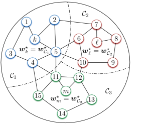
We consider a connected network consisting of N𝑁N nodes grouped into Q𝑄Q clusters, as illustrated in Figure 1. The problem is to estimate an L×1𝐿1L\times 1 unknown vector 𝒘ksubscriptsuperscript𝒘𝑘\boldsymbol{w}^{\star}_{k} at each node k𝑘k from collected data. Node k𝑘k has access to temporal measurement sequences {dk(i),𝒙k(i)}subscript𝑑𝑘𝑖subscript𝒙𝑘𝑖\{d_{k}(i),\boldsymbol{x}_{k}(i)\}, where dk(i)subscript𝑑𝑘𝑖d_{k}(i) is a scalar zero-mean reference signal, and 𝒙k(i)subscript𝒙𝑘𝑖\boldsymbol{x}_{k}(i) is an L×1𝐿1L\times 1 regression vector with a positive-definite covariance matrix 𝑹x,k=E{𝒙k(i)𝒙k(i)}>0subscript𝑹𝑥𝑘𝐸subscript𝒙𝑘𝑖superscriptsubscript𝒙𝑘top𝑖0\boldsymbol{R}_{x,k}=E\{\boldsymbol{x}_{k}(i)\boldsymbol{x}_{k}^{\top}(i)\}>0. The data at node k𝑘k are assumed to be related via the linear regression model

dk(i)=𝒙k(i)𝒘k+zk(i),subscript𝑑𝑘𝑖superscriptsubscript𝒙𝑘top𝑖superscriptsubscript𝒘𝑘subscript𝑧𝑘𝑖d_{k}(i)=\boldsymbol{x}_{k}^{\top}(i)\,\boldsymbol{w}_{k}^{\star}+z_{k}(i), (1)

where zk(i)subscript𝑧𝑘𝑖z_{k}(i) is a zero-mean i.i.d. noise of variance σz,k2superscriptsubscript𝜎𝑧𝑘2\sigma_{z,k}^{2} that is independent of any other signal. We assume that nodes belonging to the same cluster have the same parameter vector to estimate, namely,

𝒘k=𝒘𝒞q,wheneverk𝒞q.formulae-sequencesubscriptsuperscript𝒘𝑘subscriptsuperscript𝒘subscript𝒞𝑞whenever𝑘subscript𝒞𝑞\boldsymbol{w}^{\star}_{k}=\boldsymbol{w}^{\star}_{{{\mathcal{C}}}_{q}},\quad\text{whenever}\quad k\in{{\mathcal{C}}}_{q}. (2)

We say that two clusters are connected if there exists at least one edge linking a node from one cluster to a node in the other cluster. We also assume that relationships between connected clusters exist so that cooperation among adjacent clusters is beneficial. In particular, we suppose that the parameter vectors corresponding to two connected clusters 𝒞psubscript𝒞𝑝{{\mathcal{C}}}_{p} and 𝒞qsubscript𝒞𝑞{{\mathcal{C}}}_{q} satisfy certain properties, such as being close to each other [27]. Cooperation across these clusters can therefore be beneficial to infer 𝒘𝒞psubscriptsuperscript𝒘subscript𝒞𝑝\boldsymbol{w}^{\star}_{{{\mathcal{C}}}_{p}} and 𝒘𝒞qsubscriptsuperscript𝒘subscript𝒞𝑞\boldsymbol{w}^{\star}_{{{\mathcal{C}}}_{q}}.

Refer to caption
Figure 1: Clustered network consisting of 333 clusters. Two clusters are connected if they share at least one edge.

Consider the cluster 𝒞(k)𝒞𝑘{{\mathcal{C}}}(k) to which node k𝑘k belongs. A local cost function, Jk(𝒘𝒞(k))subscript𝐽𝑘subscript𝒘𝒞𝑘J_{k}(\boldsymbol{w}_{{{\mathcal{C}}}(k)}), is associated with node k𝑘k. It is assumed to be strongly convex and second-order differentiable, an example of which is the mean-square error criterion considered throughout this paper and defined by

Jk(𝒘𝒞(k))=𝔼{|dk(i)𝒙k(i)𝒘𝒞(k)|2}.subscript𝐽𝑘subscript𝒘𝒞𝑘𝔼superscriptsubscript𝑑𝑘𝑖superscriptsubscript𝒙𝑘top𝑖subscript𝒘𝒞𝑘2J_{k}(\boldsymbol{w}_{{{\mathcal{C}}}(k)})=\mathbb{E}\{|d_{k}(i)-\boldsymbol{x}_{k}^{\top}(i)\,\boldsymbol{w}_{{{\mathcal{C}}}(k)}|^{2}\}. (3)

Depending on the application, there may be certain properties among the optimal vectors {𝒘𝒞1,,𝒘𝒞Q}superscriptsubscript𝒘subscript𝒞1superscriptsubscript𝒘subscript𝒞𝑄\{\boldsymbol{w}_{{{\mathcal{C}}}_{1}}^{\star},\ldots,\boldsymbol{w}_{{{\mathcal{C}}}_{Q}}^{\star}\} that deserve to be promoted in order to enhance estimation accuracy. Among other possible options, a smoothness condition was enforced in [27]. Specifically, the local variation of the graph signal at node k𝑘k was defined as the squared 2subscript2\ell_{2}-norm of the graph gradient at this node [45], namely,

k𝒲2=𝒩kρk𝒘k𝒘2superscriptnormsubscript𝑘𝒲2subscriptsubscript𝒩𝑘subscript𝜌𝑘superscriptnormsubscript𝒘𝑘subscript𝒘2\|\nabla_{k}{\mathcal{W}}\|^{2}=\sum_{\ell\in{{\mathcal{N}}}_{k}}\rho_{k\ell}\|\boldsymbol{w}_{k}-\boldsymbol{w}_{\ell}\|^{2} (4)

where ρksubscript𝜌𝑘\rho_{k\ell} is a nonnegative weight assigned to the edge between nodes k𝑘k and \ell. As an alternative to (4) and in order to promote piecewise constant transitions in the entries of the parameter vectors, the use of the 1subscript1\ell_{1}-norm of the graph gradient at each node was also proposed and studied in [28]. In this paper, we will focus on (4).

To estimate the unknown parameter vectors 𝒘𝒞1,,𝒘𝒞Qsubscriptsuperscript𝒘subscript𝒞1subscriptsuperscript𝒘subscript𝒞𝑄\boldsymbol{w}^{\star}_{{{\mathcal{C}}}_{1}},\ldots,\boldsymbol{w}^{\star}_{{{\mathcal{C}}}_{Q}}, it was shown in [27] that the local cost (3) and the regularizer (4) can be combined at the level of each cluster. This formulation led to the following estimation problem defined in terms of Q𝑄Q Nash equilibrium problems [46], where each cluster 𝒞jsubscript𝒞𝑗{{\mathcal{C}}}_{j} estimates 𝒘𝒞jsubscriptsuperscript𝒘subscript𝒞𝑗\boldsymbol{w}^{\star}_{{{\mathcal{C}}}_{j}} by minimizing the regularized cost function J𝒞j(𝒘𝒞j,𝒘𝒞j)subscript𝐽subscript𝒞𝑗subscript𝒘subscript𝒞𝑗subscript𝒘subscript𝒞𝑗{J_{{{\mathcal{C}}}_{j}}}(\boldsymbol{w}_{{{\mathcal{C}}}_{j}},\boldsymbol{w}_{-{{\mathcal{C}}}_{j}}):

(𝒫j){min𝒘𝒞jJ𝒞j(𝒘𝒞j,𝒘𝒞j)with J𝒞j(𝒘𝒞j,𝒘𝒞j)=k𝒞j𝔼{|dk(i)𝒙k(i)𝒘𝒞(k)|2}+ηk𝒞j𝒩k\𝒞jρk𝒘𝒞(k)𝒘𝒞()2({\mathcal{P}}_{j})\left\{\begin{split}&\min_{\boldsymbol{w}_{{{\mathcal{C}}}_{j}}}{J_{{{\mathcal{C}}}_{j}}}(\boldsymbol{w}_{{{\mathcal{C}}}_{j}},\boldsymbol{w}_{-{{\mathcal{C}}}_{j}})\\ &\text{with }\;{J_{{{\mathcal{C}}}_{j}}}(\boldsymbol{w}_{{{\mathcal{C}}}_{j}},\boldsymbol{w}_{-{{\mathcal{C}}}_{j}})\\ &\qquad\quad=\sum_{k\in{{\mathcal{C}}}_{j}}\mathbb{E}\{|d_{k}(i)-\boldsymbol{x}_{k}^{\top}(i)\,\boldsymbol{w}_{{{\mathcal{C}}}(k)}|^{2}\}\\ &\qquad\quad+\eta\,\sum_{k\in{{\mathcal{C}}}_{j}}\sum_{\ell\in{{\mathcal{N}}}_{k}\backslash{{\mathcal{C}}}_{j}}\rho_{k\ell}\,\|\boldsymbol{w}_{{{\mathcal{C}}}(k)}-\boldsymbol{w}_{{{\mathcal{C}}}(\ell)}\|^{2}\end{split}\right. (5)

for j=1,,Q𝑗1𝑄j=1,\dots,Q. Note that we have kept the notation 𝒘𝒞(k)subscript𝒘𝒞𝑘\boldsymbol{w}_{{{\mathcal{C}}}(k)} in (5) to make the role of the regularization term clearer, even though we have 𝒘𝒞(k)=𝒘𝒞jsubscript𝒘𝒞𝑘subscript𝒘subscript𝒞𝑗\boldsymbol{w}_{{{\mathcal{C}}}(k)}=\boldsymbol{w}_{{{\mathcal{C}}}_{j}} for all k𝑘k in 𝒞jsubscript𝒞𝑗{{\mathcal{C}}}_{j}. The notation 𝒘𝒞jsubscript𝒘subscript𝒞𝑗\boldsymbol{w}_{-{{\mathcal{C}}}_{j}} denotes the collection of weight vectors estimated by the other clusters, that is, 𝒘𝒞j={𝒘𝒞q:q=1,,Q}{𝒘𝒞j}subscript𝒘subscript𝒞𝑗conditional-setsubscript𝒘subscript𝒞𝑞𝑞1𝑄subscript𝒘subscript𝒞𝑗\boldsymbol{w}_{-{{\mathcal{C}}}_{j}}=\{\boldsymbol{w}_{{{\mathcal{C}}}_{q}}:q=1,\ldots,Q\}\setminus\{\boldsymbol{w}_{{{\mathcal{C}}}_{j}}\}. The second term on the RHS of expression (5) enforces smoothness of the resulting graph parameter vectors {𝒘𝒞1,,𝒘𝒞Q}subscript𝒘subscript𝒞1subscript𝒘subscript𝒞𝑄\{\boldsymbol{w}_{{{\mathcal{C}}}_{1}},\ldots,\boldsymbol{w}_{{{\mathcal{C}}}_{Q}}\}, with strength parameter η0𝜂0\eta\geq 0. In [27], the coefficients {ρk}subscript𝜌𝑘\{\rho_{k\ell}\} were chosen to satisfy the conditions:

𝒩k𝒞(k)ρk=1, and {ρk>0, if 𝒩k𝒞(k),ρkk0,ρk=0, otherwise.subscriptsubscript𝒩𝑘𝒞superscript𝑘subscript𝜌𝑘1 and casesformulae-sequencesubscript𝜌𝑘0 if subscript𝒩𝑘𝒞𝑘missing-subexpressionsubscript𝜌𝑘𝑘0missing-subexpressionsubscript𝜌𝑘0 otherwise.missing-subexpression\sum_{\ell\in{{\mathcal{N}}}_{k}\setminus{{\mathcal{C}}}(k)^{-}}\rho_{k\ell}=1,\text{ and }\left\{\begin{array}[]{lr}\rho_{k\ell}>0,\text{ if }\ell\in{{\mathcal{N}}}_{k}\setminus{{\mathcal{C}}}(k),\\ \rho_{kk}\geq 0,\\ \rho_{k\ell}=0,\text{ otherwise.}\end{array}\right. (6)

We impose ρk=0subscript𝜌𝑘0\rho_{k\ell}=0 for all 𝒩k𝒞(k)subscript𝒩𝑘𝒞𝑘\ell\notin{{\mathcal{N}}}_{k}\setminus{{\mathcal{C}}}(k) since nodes belonging to the same cluster estimate the same parameter vector.

Following the same line of reasoning from [16, 18] in the single-task case, and extending the argument to problem (5) by using Nash-equilibrium properties [46, 47], the following diffusion strategy of the adapt-then-combine (ATC) form was derived in [27] for solving the multitask learning problem (5) in a distributed manner:

{𝝍k(i+1)=𝒘k(i)+μk𝒙k(i)(dk(i)𝒙k(i)𝒘k(i))+ημk(𝒩k𝒞(k)ρk(𝒘(i)𝒘k(i))),𝒘k(i+1)=𝒩k𝒞(k)ak𝝍(i+1).\left\{\begin{split}\boldsymbol{\psi}_{k}(i+1)&=\boldsymbol{w}_{k}(i)+\mu_{k}\,\boldsymbol{x}_{k}(i)\,(d_{k}(i)-\boldsymbol{x}_{k}^{\top}(i)\,\boldsymbol{w}_{k}(i))\\ &\quad+\eta\,\mu_{k}\Big{(}\sum_{\ell\in{{\mathcal{N}}}_{k}\setminus{{\mathcal{C}}}(k)^{-}}\rho_{k\ell}(\boldsymbol{w}_{\ell}(i)-\boldsymbol{w}_{k}(i))\Big{)},\\ \boldsymbol{w}_{k}(i+1)&=\sum_{\ell\in{{\mathcal{N}}}_{k}\cap{{\mathcal{C}}}(k)}a_{\ell k}\,\boldsymbol{\psi}_{\ell}(i+1).\end{split}\right. (7)

where 𝒘k(i)subscript𝒘𝑘𝑖\boldsymbol{w}_{k}(i) denotes the estimate of the unknown parameter vector 𝒘ksubscriptsuperscript𝒘𝑘\boldsymbol{w}^{\star}_{k} at node k𝑘k and iteration i𝑖i, and μksubscript𝜇𝑘\mu_{k} is a positive step-size parameter. The combination coefficients {ak}subscript𝑎𝑘\{a_{\ell k}\} are nonnegative scalars that are chosen to satisfy the conditions:

𝒩k𝒞(k)ak=1, and {ak>0, if 𝒩k𝒞(k),ak=0, otherwise.subscriptsubscript𝒩𝑘𝒞𝑘subscript𝑎𝑘1 and casesformulae-sequencesubscript𝑎𝑘0 if subscript𝒩𝑘𝒞𝑘missing-subexpressionsubscript𝑎𝑘0 otherwise.missing-subexpression\sum_{\ell\in{{\mathcal{N}}}_{k}\cap{{\mathcal{C}}}(k)}a_{\ell k}=1,\text{ and }\left\{\begin{array}[]{lr}a_{\ell k}>0,\text{ if }\ell\in{{\mathcal{N}}}_{k}\cap{{\mathcal{C}}}(k),\\ a_{\ell k}=0,\text{ otherwise.}\end{array}\right. (8)

There are several ways to select these coefficients such as using the averaging rule or the Metropolis rule (see [16] for a listing of these and other choices).

II-B Asynchronous multitask diffusion adaptation

To model the asynchronous behavior over networks, we follow the same procedure developed in [42] since the model presented in that work allows us to cover many situations of practical interest. Specifically, we replace each deterministic step-size μksubscript𝜇𝑘\mu_{k} by a random process μk(i)subscript𝜇𝑘𝑖\mu_{k}(i), and model uncertainties in the links by using random combination coefficients {ak(i)}subscript𝑎𝑘𝑖\{a_{\ell k}(i)\} and random regularization factors {ρk(i)}subscript𝜌𝑘𝑖\{\rho_{k\ell}(i)\}. In other words, we modify the multitask diffusion strategy (7) to the following form:

{𝝍k(i+1)=𝒘k(i)+μk(i)𝒙k(i)(dk(i)𝒙k(i)𝒘k(i))+ημk(i)(𝒩k(i)𝒞(k)ρk(i)(𝒘(i)𝒘k(i))),𝒘k(i+1)=𝒩k(i)𝒞(k)ak(i)𝝍(i+1)\left\{\begin{split}\boldsymbol{\psi}_{k}(i+1)&=\boldsymbol{w}_{k}(i)+\mu_{k}(i)\,\boldsymbol{x}_{k}(i)\,(d_{k}(i)-\boldsymbol{x}_{k}^{\top}(i)\,\boldsymbol{w}_{k}(i))\\ &\quad+\eta\,\mu_{k}(i)\Big{(}\sum_{\ell\in{{\mathcal{N}}}_{k}(i)\setminus{{\mathcal{C}}}(k)^{-}}\rho_{k\ell}(i)(\boldsymbol{w}_{\ell}(i)-\boldsymbol{w}_{k}(i))\Big{)},\\ \boldsymbol{w}_{k}(i+1)&=\sum_{\ell\in{{\mathcal{N}}}_{k}(i)\cap{{\mathcal{C}}}(k)}a_{\ell k}(i)\,\boldsymbol{\psi}_{\ell}(i+1)\end{split}\right. (9)

where 𝒩k(i)subscript𝒩𝑘𝑖{{\mathcal{N}}}_{k}(i) is also now random and denotes the random neighborhood of agent k𝑘k at time instant i𝑖i. The composition of each cluster is assumed to be known a priori and does not change over time. When dealing with multitask networks, compared to single-task networks [42], a second source of uncertainty comes from links transmitting data between clusters. Indeed, data transmitted over intra-cluster links are used to reach a consensus while data transmitted over inter-cluster links are used to promote relationships between tasks. In a manner similar to [42], the asynchronous network model is assumed to satisfy the following conditions:

  • Conditions on the step-size parameters: At each time instant i𝑖i, the step-size at node k𝑘k is a bounded nonnegative random variable μk(i)[0,μmax,k]subscript𝜇𝑘𝑖0subscript𝜇𝑘\mu_{k}(i)\in[0,\mu_{\max,k}]. These step-sizes are collected into the random matrix 𝑴(i)diag{μ1(i),,μN(i)}𝑴𝑖diagsubscript𝜇1𝑖subscript𝜇𝑁𝑖\boldsymbol{M}(i)\triangleq\text{diag}\{\mu_{1}(i),\ldots,\mu_{N}(i)\}. We assume that {𝑴(i),i0}𝑴𝑖𝑖0\{\boldsymbol{M}(i),i\geq 0\} is a weakly stationary random process with mean 𝑴¯¯𝑴\overline{\boldsymbol{M}} and Kronecker-covariance matrix 𝑪Msubscript𝑪𝑀\boldsymbol{C}_{M} of size N2×N2superscript𝑁2superscript𝑁2N^{2}\times N^{2} defined as

    𝑪M𝔼{(𝑴(i)𝑴¯)(𝑴(i)𝑴¯)}subscript𝑪𝑀𝔼tensor-product𝑴𝑖¯𝑴𝑴𝑖¯𝑴\boldsymbol{C}_{M}\triangleq\mathbb{E}\{(\boldsymbol{M}(i)-\overline{\boldsymbol{M}})\otimes(\boldsymbol{M}(i)-\overline{\boldsymbol{M}})\} (10)

    with tensor-product\otimes denoting the Kronecker product.

  • Conditions on the combination coefficients: The random coefficients {ak(i)}subscript𝑎𝑘𝑖\{a_{\ell k}(i)\} used to scale the estimates {𝝍(i+1)}subscript𝝍𝑖1\{\boldsymbol{\psi}_{\ell}(i+1)\} that are being received by node k𝑘k from its cluster neighbors 𝒩k(i)𝒞(k)subscript𝒩𝑘𝑖𝒞𝑘\ell\in{{\mathcal{N}}}_{k}(i)\cap{{\mathcal{C}}}(k) satisfy the following constraints at each iteration i𝑖i:

    𝒩k(i)𝒞(k)ak(i)=1,and{ak(i)>0,if 𝒩k(i)𝒞(k)ak(i)=0,otherwise.subscriptsubscript𝒩𝑘𝑖𝒞𝑘subscript𝑎𝑘𝑖1andcasesformulae-sequencesubscript𝑎𝑘𝑖0if subscript𝒩𝑘𝑖𝒞𝑘missing-subexpressionsubscript𝑎𝑘𝑖0otherwise.missing-subexpression\sum_{\ell\in{{\mathcal{N}}}_{k}(i)\cap{{\mathcal{C}}}(k)}a_{\ell k}(i)=1,\text{and}\left\{\begin{array}[]{lr}a_{\ell k}(i)>0,\text{if }\ell\in{{\mathcal{N}}}_{k}(i)\cap{{\mathcal{C}}}(k)\\ a_{\ell k}(i)=0,\text{otherwise.}\end{array}\right. (11)

    We collect these coefficients into the random N×N𝑁𝑁N\times N left-stochastic matrix 𝑨(i)𝑨𝑖\boldsymbol{A}(i). We again assume that {𝑨(i),i0}𝑨𝑖𝑖0\{\boldsymbol{A}(i),i\geq 0\} is a weakly stationary random process. Let 𝑨¯¯𝑨\overline{\boldsymbol{A}} be its mean and 𝑪Asubscript𝑪𝐴\boldsymbol{C}_{A} its Kronecker-covariance matrix of size N2×N2superscript𝑁2superscript𝑁2N^{2}\times N^{2} defined as

    𝑪A𝔼{(𝑨(i)𝑨¯)(𝑨(i)𝑨¯)}.subscript𝑪𝐴𝔼tensor-product𝑨𝑖¯𝑨𝑨𝑖¯𝑨\boldsymbol{C}_{A}\triangleq\mathbb{E}\{(\boldsymbol{A}(i)-\overline{\boldsymbol{A}})\otimes(\boldsymbol{A}(i)-\overline{\boldsymbol{A}})\}. (12)
  • Conditions on the regularization factors: The random factors {ρk(i)}subscript𝜌𝑘𝑖\{\rho_{k\ell}(i)\}, which adjust the regularization strength between the parameter vectors at neighboring nodes of distinct clusters, satisfy the following constraints at each iteration i𝑖i:

    𝒩k(i)𝒞(k)ρk(i)=1,and{ρk(i)>0,if 𝒩k(i)𝒞(k)ρkk(i)0,ρk(i)=0,otherwise.subscriptsubscript𝒩𝑘𝑖𝒞superscript𝑘subscript𝜌𝑘𝑖1andcasesformulae-sequencesubscript𝜌𝑘𝑖0if subscript𝒩𝑘𝑖𝒞𝑘missing-subexpressionsubscript𝜌𝑘𝑘𝑖0missing-subexpressionsubscript𝜌𝑘𝑖0otherwise.missing-subexpression\sum_{\ell\in{{\mathcal{N}}}_{k}(i)\setminus{{\mathcal{C}}}(k)^{-}}\rho_{k\ell}(i)=1,\text{and}\left\{\begin{array}[]{lr}\rho_{k\ell}(i)>0,\text{if }\ell\in{{\mathcal{N}}}_{k}(i)\setminus{{\mathcal{C}}}(k)\\ \rho_{kk}(i)\geq 0,\\ \rho_{k\ell}(i)=0,\text{otherwise.}\end{array}\right. (13)

    We collect these coefficients into the random N×N𝑁𝑁{N\times N} right-stochastic matrix 𝑷(i)𝑷𝑖\boldsymbol{P}(i). We assume that {𝑷(i),i0}𝑷𝑖𝑖0\{\boldsymbol{P}(i),i\geq 0\} is a weakly stationary random process with mean 𝑷¯¯𝑷\overline{\boldsymbol{P}} and Kronecker-covariance matrix 𝑪Psubscript𝑪𝑃\boldsymbol{C}_{P} of size N2×N2superscript𝑁2superscript𝑁2N^{2}\times N^{2} defined as

    𝑪P𝔼{(𝑷(i)𝑷¯)(𝑷(i)𝑷¯)}.subscript𝑪𝑃𝔼tensor-product𝑷𝑖¯𝑷𝑷𝑖¯𝑷\boldsymbol{C}_{P}\triangleq\mathbb{E}\{(\boldsymbol{P}(i)-\overline{\boldsymbol{P}})\otimes(\boldsymbol{P}(i)-\overline{\boldsymbol{P}})\}. (14)
  • Independence assumptions: To enable tractable analysis, we shall assume that the random matrices 𝑴(i)𝑴𝑖\boldsymbol{M}(i), 𝑨(i)𝑨𝑖\boldsymbol{A}(i), and 𝑷(i)𝑷𝑖\boldsymbol{P}(i) at iteration i𝑖i are mutually-independent and independent of any other random variables. These matrices are related to node, intra-cluster and inter-cluster link failures, respectively.

  • Mean graph: The mean matrices 𝑨¯¯𝑨\overline{\boldsymbol{A}} and 𝑷¯¯𝑷\overline{\boldsymbol{P}} define the intra-cluster and inter-cluster neighborhoods, namely, 𝒩k𝒞(k)subscript𝒩𝑘𝒞𝑘{{\mathcal{N}}}_{k}\cap{{\mathcal{C}}}(k) and 𝒩k𝒞(k)subscript𝒩𝑘𝒞𝑘{{\mathcal{N}}}_{k}\setminus{{\mathcal{C}}}(k) for all k𝑘k, respectively. We refer to the neighborhoods 𝒩k=(𝒩k𝒞(k))(𝒩k𝒞(k))subscript𝒩𝑘subscript𝒩𝑘𝒞𝑘subscript𝒩𝑘𝒞𝑘{{\mathcal{N}}}_{k}=\big{(}{{\mathcal{N}}}_{k}\cap{{\mathcal{C}}}(k)\big{)}\cup\big{(}{{\mathcal{N}}}_{k}\setminus{{\mathcal{C}}}(k)\big{)} for all k𝑘k, defined by 𝑨¯¯𝑨\overline{\boldsymbol{A}} and 𝑷¯¯𝑷\overline{\boldsymbol{P}}, as the mean graph. In view of the above conditions, the mean combination coefficients a¯k𝔼{ak(i)}subscript¯𝑎𝑘𝔼subscript𝑎𝑘𝑖\bar{a}_{\ell k}\triangleq\mathbb{E}\{a_{\ell k}(i)\} and regularization factors ρ¯k𝔼{ρk(i)}subscript¯𝜌𝑘𝔼subscript𝜌𝑘𝑖\bar{\rho}_{k\ell}\triangleq\mathbb{E}\{\rho_{k\ell}(i)\} are nonnegative and satisfy the following constraints.

    𝒩k𝒞(k)a¯k=1, and {a¯k>0, if 𝒩k𝒞(k),a¯k=0, otherwise,subscriptsubscript𝒩𝑘𝒞𝑘subscript¯𝑎𝑘1 and casesformulae-sequencesubscript¯𝑎𝑘0 if subscript𝒩𝑘𝒞𝑘missing-subexpressionsubscript¯𝑎𝑘0 otherwise,missing-subexpression\sum_{\ell\in{{\mathcal{N}}}_{k}\cap{{\mathcal{C}}}(k)}\bar{a}_{\ell k}=1,\text{ and }\left\{\begin{array}[]{lr}\bar{a}_{\ell k}>0,\text{ if }\ell\in{{\mathcal{N}}}_{k}\cap{{\mathcal{C}}}(k),\\ \bar{a}_{\ell k}=0,\text{ otherwise,}\end{array}\right. (15)
    𝒩k𝒞(k)ρ¯k=1, and {ρ¯k>0, if 𝒩k𝒞(k),ρ¯kk0,ρ¯k=0, otherwise.subscriptsubscript𝒩𝑘𝒞superscript𝑘subscript¯𝜌𝑘1 and casesformulae-sequencesubscript¯𝜌𝑘0 if subscript𝒩𝑘𝒞𝑘missing-subexpressionsubscript¯𝜌𝑘𝑘0missing-subexpressionsubscript¯𝜌𝑘0 otherwise.missing-subexpression\sum_{\ell\in{{\mathcal{N}}}_{k}\setminus{{\mathcal{C}}}(k)^{-}}\bar{\rho}_{k\ell}=1,\text{ and }\left\{\begin{array}[]{lr}\bar{\rho}_{k\ell}>0,\text{ if }\ell\in{{\mathcal{N}}}_{k}\setminus{{\mathcal{C}}}(k),\\ \bar{\rho}_{kk}\geq 0,\\ \bar{\rho}_{k\ell}=0,\text{ otherwise.}\end{array}\right. (16)

Using the same arguments as Lemmas 2 and 3 in [42], we can state the following properties for the asynchronous model (9).

Property 1.

The N×N𝑁𝑁N\times N matrix 𝐀¯¯𝐀\overline{\boldsymbol{A}} and the N2×N2superscript𝑁2superscript𝑁2N^{2}\times N^{2} matrix 𝐀¯𝐀¯+𝐂Atensor-product¯𝐀¯𝐀subscript𝐂𝐴\overline{\boldsymbol{A}}\otimes\overline{\boldsymbol{A}}+\boldsymbol{C}_{A} are left-stochastic matrices.

Property 2.

The N×N𝑁𝑁N\times N matrix 𝐏¯¯𝐏\overline{\boldsymbol{P}} and the N2×N2superscript𝑁2superscript𝑁2N^{2}\times N^{2} matrix 𝐏¯𝐏¯+𝐂Ptensor-product¯𝐏¯𝐏subscript𝐂𝑃\overline{\boldsymbol{P}}\otimes\overline{\boldsymbol{P}}+\boldsymbol{C}_{P} are right-stochastic matrices.

Property 3.

For every node k𝑘k, the neighborhood 𝒩ksubscript𝒩𝑘{{\mathcal{N}}}_{k} that is defined by the mean graph of the asynchronous model (9) is equal to the union of all possible realizations for the random neighborhood 𝒩k(i)=(𝒩k(i)𝒞(k))(𝒩k(i)𝒞(k))subscript𝒩𝑘𝑖subscript𝒩𝑘𝑖𝒞𝑘subscript𝒩𝑘𝑖𝒞𝑘{{\mathcal{N}}}_{k}(i)=\big{(}{{\mathcal{N}}}_{k}(i)\cap{{\mathcal{C}}}(k)\big{)}\cup\big{(}{{\mathcal{N}}}_{k}(i)\setminus{{\mathcal{C}}}(k)\big{)}

.

We provide in Appendix A one example for a common asynchronous network referred to as the Bernoulli network. The Bernoulli model proposed in [42] is more general than the one used for modeling random link failures in consensus networks [37, 8] since it also allows to consider random “on-off” behavior for agents. When dealing with multitask problems over asynchronous network, additional sources of uncertainties must be considered. The network provided in Appendix A allows us to jointly model intra-cluster link failures, inter-cluster link failures, and random “on-off” behaviors for agents.

III Performance of multitask diffusion over asynchronous networks

The performance of the multitask diffusion algorithm (9) is affected by various random perturbations due to the asynchronous events. We now examine the stochastic behavior of this strategy in the mean and mean-square error sense.

III-A Mean error behavior analysis

For each agent k𝑘k, we introduce the weight error vectors:

𝒘~k(i)𝒘k𝒘k(i),𝝍~k(i)𝒘k𝝍k(i)formulae-sequencesubscript~𝒘𝑘𝑖superscriptsubscript𝒘𝑘subscript𝒘𝑘𝑖subscript~𝝍𝑘𝑖superscriptsubscript𝒘𝑘subscript𝝍𝑘𝑖\widetilde{\boldsymbol{w}}_{k}(i)\triangleq\boldsymbol{w}_{k}^{\star}-\boldsymbol{w}_{k}(i),\quad\quad\quad\widetilde{\boldsymbol{\psi}}_{k}(i)\triangleq\boldsymbol{w}_{k}^{\star}-\boldsymbol{\psi}_{k}(i) (17)

where 𝒘ksuperscriptsubscript𝒘𝑘\boldsymbol{w}_{k}^{\star} is the optimum parameter vector at node k𝑘k. We denote by 𝒘~(i)~𝒘𝑖\widetilde{\boldsymbol{w}}(i), 𝝍~(i)~𝝍𝑖\widetilde{\boldsymbol{\psi}}(i), and 𝒘superscript𝒘\boldsymbol{w}^{\star} the block weight error vector, the block intermediate weight error vector, and the block optimum weight vector, all of size N×1𝑁1N\times 1 with blocks of size L×1𝐿1L\times 1, namely,

𝒘~(i)~𝒘𝑖\displaystyle\widetilde{\boldsymbol{w}}(i) \displaystyle\triangleq col{𝒘~1(i),,𝒘~N(i)}colsubscript~𝒘1𝑖subscript~𝒘𝑁𝑖\displaystyle\text{col}\{\widetilde{\boldsymbol{w}}_{1}(i),\ldots,\widetilde{\boldsymbol{w}}_{N}(i)\} (18)
𝝍~(i)~𝝍𝑖\displaystyle\widetilde{\boldsymbol{\psi}}(i) \displaystyle\triangleq col{𝝍~1(i),,𝝍~N(i)}colsubscript~𝝍1𝑖subscript~𝝍𝑁𝑖\displaystyle\text{col}\{\widetilde{\boldsymbol{\psi}}_{1}(i),\ldots,\widetilde{\boldsymbol{\psi}}_{N}(i)\} (19)
𝒘superscript𝒘\displaystyle\boldsymbol{w}^{\star} \displaystyle\triangleq col{𝒘1,,𝒘N}.colsuperscriptsubscript𝒘1superscriptsubscript𝒘𝑁\displaystyle\text{col}\{\boldsymbol{w}_{1}^{\star},\ldots,\boldsymbol{w}_{N}^{\star}\}. (20)

We also introduce the following N×N𝑁𝑁N\times N block matrices with individual entries of size L×L𝐿𝐿L\times L:

𝓜(i)𝓜𝑖\displaystyle{\boldsymbol{{\mathcal{M}}}}(i) \displaystyle\triangleq 𝑴(i)𝑰Ltensor-product𝑴𝑖subscript𝑰𝐿\displaystyle\boldsymbol{M}(i)\otimes\boldsymbol{I}_{L} (21)
𝓐(i)𝓐𝑖\displaystyle{\boldsymbol{{\mathcal{A}}}}(i) \displaystyle\triangleq 𝑨(i)𝑰Ltensor-product𝑨𝑖subscript𝑰𝐿\displaystyle\boldsymbol{A}(i)\otimes\boldsymbol{I}_{L} (22)
𝓟(i)𝓟𝑖\displaystyle{\boldsymbol{{\mathcal{P}}}}(i) \displaystyle\triangleq 𝑷(i)𝑰L.tensor-product𝑷𝑖subscript𝑰𝐿\displaystyle\boldsymbol{P}(i)\otimes\boldsymbol{I}_{L}. (23)

To perform the theoretical analysis, we introduce the following independence assumption.

Assumption 1.

(Independent regressors) The regression vectors 𝐱k(i)subscript𝐱𝑘𝑖\boldsymbol{x}_{k}(i) arise from a stationary random process that is temporally stationary, temporally white, and independent over space with 𝐑x,k=E{𝐱k(i)𝐱k(i)}>0subscript𝐑𝑥𝑘𝐸subscript𝐱𝑘𝑖subscriptsuperscript𝐱top𝑘𝑖0\boldsymbol{R}_{x,k}=E\{\boldsymbol{x}_{k}(i)\,\boldsymbol{x}^{\top}_{k}(i)\}>0.

A direct consequence is that 𝒙k(i)subscript𝒙𝑘𝑖\boldsymbol{x}_{k}(i) is independent of 𝒘~(j)subscript~𝒘𝑗\widetilde{\boldsymbol{w}}_{\ell}(j) for all \ell and ji𝑗𝑖j\leq i. Although not true in general, this assumption is commonly used to analyze adaptive constructions since it allows to simplify the derivations without constraining the conclusions. There are several results in the adaptation literature that show that performance results that are obtained under the above independence assumptions match well the actual performance of the algorithms when the step-sizes are sufficiently small (see, e.g., [48, App. 24.A] and the many references therein).

The estimation error in the first step of the asynchronous strategy (9) can be rewritten as:

dk(i)𝒙k(i)𝒘k(i)=𝒙k(i)𝒘~k(i)+zk(i).subscript𝑑𝑘𝑖superscriptsubscript𝒙𝑘top𝑖subscript𝒘𝑘𝑖superscriptsubscript𝒙𝑘top𝑖subscript~𝒘𝑘𝑖subscript𝑧𝑘𝑖d_{k}(i)-\boldsymbol{x}_{k}^{\top}(i)\boldsymbol{w}_{k}(i)=\boldsymbol{x}_{k}^{\top}(i)\widetilde{\boldsymbol{w}}_{k}(i)+z_{k}(i). (24)

Subtracting 𝒘ksubscriptsuperscript𝒘𝑘\boldsymbol{w}^{\star}_{k} from both sides of the adaptation step in (9) and using the above relation, we can express the update equation for 𝝍~(i+1)~𝝍𝑖1\widetilde{\boldsymbol{\psi}}(i+1) as:

𝝍~(i+1)=[𝑰NL𝓜(i)(𝓡x(i)+η𝓠(i))]𝒘~(i)𝓜(i)𝒑xz(i)+η𝓜(i)𝓠(i)𝒘~𝝍𝑖1delimited-[]subscript𝑰𝑁𝐿𝓜𝑖subscript𝓡𝑥𝑖𝜂𝓠𝑖~𝒘𝑖𝓜𝑖subscript𝒑𝑥𝑧𝑖𝜂𝓜𝑖𝓠𝑖superscript𝒘\begin{split}\widetilde{\boldsymbol{\psi}}(i+1)=&[\boldsymbol{I}_{NL}-{\boldsymbol{{\mathcal{M}}}}(i)({\boldsymbol{\mathcal{R}}}_{x}(i)+\eta\,{\boldsymbol{\mathcal{Q}}}(i))]\widetilde{\boldsymbol{w}}(i)-\\ &{\boldsymbol{{\mathcal{M}}}}(i)\boldsymbol{p}_{xz}(i)+\eta\,{\boldsymbol{{\mathcal{M}}}}(i){\boldsymbol{\mathcal{Q}}}(i)\boldsymbol{w}^{\star}\end{split} (25)

where

𝓠(i)𝑰NL𝓟(i),𝓠𝑖subscript𝑰𝑁𝐿𝓟𝑖{\boldsymbol{\mathcal{Q}}}(i)\triangleq\boldsymbol{I}_{NL}-{\boldsymbol{{\mathcal{P}}}}(i), (26)

while 𝓡x(i)subscript𝓡𝑥𝑖{\boldsymbol{\mathcal{R}}}_{x}(i) is an N×N𝑁𝑁N\times N block matrix with individual entries of size L×L𝐿𝐿L\times L given by

𝓡x(i)diag{𝒙1(i)𝒙1(i),,𝒙N(i)𝒙N(i)},subscript𝓡𝑥𝑖diagsubscript𝒙1𝑖subscriptsuperscript𝒙top1𝑖subscript𝒙𝑁𝑖subscriptsuperscript𝒙top𝑁𝑖{\boldsymbol{\mathcal{R}}}_{x}(i)\triangleq\text{diag}\big{\{}\boldsymbol{x}_{1}(i)\boldsymbol{x}^{\top}_{1}(i),\ldots,\boldsymbol{x}_{N}(i)\boldsymbol{x}^{\top}_{N}(i)\big{\}}, (27)

and 𝒑xz(i)subscript𝒑𝑥𝑧𝑖\boldsymbol{p}_{xz}(i) is the N×1𝑁1N\times 1 block column vector with blocks of size L×1𝐿1L\times 1 defined as

𝒑xz(i)col{𝒙1(i)z1(i),,𝒙N(i)zN(i)}.subscript𝒑𝑥𝑧𝑖colsubscript𝒙1𝑖subscript𝑧1𝑖subscript𝒙𝑁𝑖subscript𝑧𝑁𝑖\boldsymbol{p}_{xz}(i)\triangleq\text{col}\{\boldsymbol{x}_{1}(i)z_{1}(i),\ldots,\boldsymbol{x}_{N}(i)z_{N}(i)\}. (28)

Subtracting 𝒘ksubscriptsuperscript𝒘𝑘\boldsymbol{w}^{\star}_{k} from both sides of the combination step in (9), we get the block weight error vector:

𝒘~(i+1)=𝓐(i)𝝍~(i+1).~𝒘𝑖1superscript𝓐top𝑖~𝝍𝑖1\widetilde{\boldsymbol{w}}(i+1)={\boldsymbol{{\mathcal{A}}}}^{\top}(i)\,\widetilde{\boldsymbol{\psi}}(i+1). (29)

Substituting (25) into (29) we find that the error dynamics of the asynchronous multitask diffusion strategy (9) evolves according to the following recursion:

𝒘~(i+1)=𝓐(i)[𝑰NL𝓜(i)(𝓡x(i)+η𝓠(i))]𝒘~(i)𝓐(i)𝓜(i)𝒑xz(i)+η𝓐(i)𝓜(i)𝓠(i)𝒘.~𝒘𝑖1superscript𝓐top𝑖delimited-[]subscript𝑰𝑁𝐿𝓜𝑖subscript𝓡𝑥𝑖𝜂𝓠𝑖~𝒘𝑖superscript𝓐top𝑖𝓜𝑖subscript𝒑𝑥𝑧𝑖𝜂superscript𝓐top𝑖𝓜𝑖𝓠𝑖superscript𝒘\begin{split}\widetilde{\boldsymbol{w}}(i+1)=&{\boldsymbol{{\mathcal{A}}}}^{\top}(i)\big{[}\boldsymbol{I}_{NL}-{\boldsymbol{{\mathcal{M}}}}(i)({\boldsymbol{\mathcal{R}}}_{x}(i)+\eta\,{\boldsymbol{\mathcal{Q}}}(i))\big{]}\widetilde{\boldsymbol{w}}(i)-\\ &{\boldsymbol{{\mathcal{A}}}}^{\top}(i){\boldsymbol{{\mathcal{M}}}}(i)\boldsymbol{p}_{xz}(i)+\eta\,{\boldsymbol{{\mathcal{A}}}}^{\top}(i){\boldsymbol{{\mathcal{M}}}}(i){\boldsymbol{\mathcal{Q}}}(i)\boldsymbol{w}^{\star}.\end{split} (30)

For compactness of notation, we introduce the symbols:

𝓑(i)𝓑𝑖\displaystyle{\boldsymbol{\mathcal{B}}}(i) \displaystyle\triangleq 𝓐(i)[𝑰NL𝓜(i)(𝓡x(i)+η𝓠(i))]superscript𝓐top𝑖delimited-[]subscript𝑰𝑁𝐿𝓜𝑖subscript𝓡𝑥𝑖𝜂𝓠𝑖\displaystyle{\boldsymbol{{\mathcal{A}}}}^{\top}(i)\big{[}\boldsymbol{I}_{NL}-{\boldsymbol{{\mathcal{M}}}}(i)({\boldsymbol{\mathcal{R}}}_{x}(i)+\eta\,{\boldsymbol{\mathcal{Q}}}(i))\big{]} (31)
𝒈(i)𝒈𝑖\displaystyle\boldsymbol{g}(i) \displaystyle\triangleq 𝓐(i)𝓜(i)𝒑xz(i)superscript𝓐top𝑖𝓜𝑖subscript𝒑𝑥𝑧𝑖\displaystyle{\boldsymbol{{\mathcal{A}}}}^{\top}(i){\boldsymbol{{\mathcal{M}}}}(i)\,\boldsymbol{p}_{xz}(i) (32)
𝒓(i)𝒓𝑖\displaystyle\boldsymbol{r}(i) \displaystyle\triangleq 𝓐(i)𝓜(i)𝑸(i)𝒘,superscript𝓐top𝑖𝓜𝑖𝑸𝑖superscript𝒘\displaystyle{\boldsymbol{{\mathcal{A}}}}^{\top}(i){\boldsymbol{{\mathcal{M}}}}(i)\boldsymbol{Q}(i)\,\boldsymbol{w}^{\star}, (33)

so that (30) can be written as

𝒘~(i+1)=𝓑(i)𝒘~(i)𝒈(i)+η𝒓(i).~𝒘𝑖1𝓑𝑖~𝒘𝑖𝒈𝑖𝜂𝒓𝑖\widetilde{\boldsymbol{w}}(i+1)={\boldsymbol{{\mathcal{B}}}}(i)\,\widetilde{\boldsymbol{w}}(i)-\boldsymbol{g}(i)+\eta\boldsymbol{r}(i). (34)

Taking the expectation of both sides, using Assumption 1, and the independence of 𝑨(i)𝑨𝑖\boldsymbol{A}(i), 𝑴(i)𝑴𝑖\boldsymbol{M}(i), and 𝑷(i)𝑷𝑖\boldsymbol{P}(i), the network mean error vector ends up evolving according to the following dynamics:

𝔼{𝒘~(i+1)}=𝓑𝔼{𝒘~(i)}+η𝒓𝔼~𝒘𝑖1𝓑𝔼~𝒘𝑖𝜂𝒓\mathbb{E}\{\widetilde{\boldsymbol{w}}(i+1)\}={{\boldsymbol{\mathcal{B}}}}\,\mathbb{E}\{\widetilde{\boldsymbol{w}}(i)\}+\eta\boldsymbol{r} (35)

where

𝓑𝓑\displaystyle{\boldsymbol{\mathcal{B}}} \displaystyle\triangleq 𝔼{𝓑(i)}=𝓐[𝑰NL𝓜(𝓡x+η𝓠)]𝔼𝓑𝑖superscript𝓐topdelimited-[]subscript𝑰𝑁𝐿𝓜subscript𝓡𝑥𝜂𝓠\displaystyle\mathbb{E}\{{\boldsymbol{\mathcal{B}}}(i)\}={\boldsymbol{\mathcal{A}}}^{\top}\big{[}\boldsymbol{I}_{NL}-{\boldsymbol{\mathcal{M}}}({\boldsymbol{\mathcal{R}}}_{x}+\eta{\boldsymbol{\mathcal{Q}}})\big{]} (36)
𝒓𝒓\displaystyle\boldsymbol{r} \displaystyle\triangleq 𝔼{𝒓(i)}=𝓐𝓜𝓠𝒘,𝔼𝒓𝑖superscript𝓐top𝓜𝓠superscript𝒘\displaystyle\mathbb{E}\{\boldsymbol{r}(i)\}={\boldsymbol{\mathcal{A}}}^{\top}{\boldsymbol{\mathcal{M}}}{\boldsymbol{\mathcal{Q}}}\,\boldsymbol{w}^{\star}, (37)

where 𝓐𝓐{\boldsymbol{\mathcal{A}}}, 𝓜𝓜{\boldsymbol{\mathcal{M}}}, 𝓡xsubscript𝓡𝑥{\boldsymbol{\mathcal{R}}}_{x}, and 𝓠𝓠{\boldsymbol{\mathcal{Q}}} denote the expectations of 𝓐(i)𝓐𝑖{\boldsymbol{\mathcal{A}}}(i), 𝓜(i)𝓜𝑖{\boldsymbol{\mathcal{M}}}(i), 𝓡x(i)subscript𝓡𝑥𝑖{\boldsymbol{\mathcal{R}}}_{x}(i), and 𝓠(i)𝓠𝑖{\boldsymbol{\mathcal{Q}}}(i), respectively, and are given by:

𝓐𝓐\displaystyle{\boldsymbol{\mathcal{A}}} \displaystyle\triangleq 𝔼{𝓐(i)}=𝑨¯𝑰L𝔼𝓐𝑖tensor-product¯𝑨subscript𝑰𝐿\displaystyle\mathbb{E}\{{\boldsymbol{\mathcal{A}}}(i)\}=\overline{\boldsymbol{A}}\otimes\boldsymbol{I}_{L} (38)
𝓜𝓜\displaystyle{\boldsymbol{\mathcal{M}}} \displaystyle\triangleq 𝔼{𝓜(i)}=𝑴¯𝑰L𝔼𝓜𝑖tensor-product¯𝑴subscript𝑰𝐿\displaystyle\mathbb{E}\{{\boldsymbol{\mathcal{M}}}(i)\}=\overline{\boldsymbol{M}}\otimes\boldsymbol{I}_{L} (39)
𝓟𝓟\displaystyle{\boldsymbol{\mathcal{P}}} \displaystyle\triangleq 𝔼{𝓟(i)}=𝑷¯𝑰L𝔼𝓟𝑖tensor-product¯𝑷subscript𝑰𝐿\displaystyle\mathbb{E}\{{\boldsymbol{\mathcal{P}}}(i)\}=\overline{\boldsymbol{P}}\otimes\boldsymbol{I}_{L} (40)
𝓡xsubscript𝓡𝑥\displaystyle{\boldsymbol{\mathcal{R}}}_{x} \displaystyle\triangleq 𝔼{𝓡x(i)}=diag{𝑹x,1,,𝑹x,N}𝔼subscript𝓡𝑥𝑖diagsubscript𝑹𝑥1subscript𝑹𝑥𝑁\displaystyle\mathbb{E}\{{\boldsymbol{\mathcal{R}}}_{x}(i)\}=\text{diag}\{\boldsymbol{R}_{x,1},\ldots,\boldsymbol{R}_{x,N}\} (41)
𝓠𝓠\displaystyle{\boldsymbol{\mathcal{Q}}} \displaystyle\triangleq 𝔼{𝓠(i)}=𝑰NL𝔼{𝓟(i)}=𝑰NL𝓟.𝔼𝓠𝑖subscript𝑰𝑁𝐿𝔼𝓟𝑖subscript𝑰𝑁𝐿𝓟\displaystyle\mathbb{E}\{{\boldsymbol{\mathcal{Q}}}(i)\}=\boldsymbol{I}_{NL}-\mathbb{E}\{{\boldsymbol{\mathcal{P}}}(i)\}=\boldsymbol{I}_{NL}-{\boldsymbol{\mathcal{P}}}. (42)

Note that 𝔼{𝒈(i)}=0𝔼𝒈𝑖0\mathbb{E}\{\boldsymbol{g}(i)\}=0 since zk(i)subscript𝑧𝑘𝑖z_{k}(i) is zero-mean and independent of any other signal.

Theorem 1.

(Stability in the mean) Assume data model (1) and Assumption 1 hold. Then, for any initial condition, the multitask diffusion LMS strategy (9) applied to asynchronous networks converges asymptotically in the mean if, and only if, the step-sizes in 𝓜𝓜{\boldsymbol{\mathcal{M}}} are chosen to satisfy

ρ(𝓐[𝑰NL𝓜(𝓡x+η𝓠)])<1,𝜌superscript𝓐topdelimited-[]subscript𝑰𝑁𝐿𝓜subscript𝓡𝑥𝜂𝓠1\rho\big{(}{\boldsymbol{\mathcal{A}}}^{\top}\big{[}\boldsymbol{I}_{NL}-{\boldsymbol{\mathcal{M}}}({\boldsymbol{\mathcal{R}}}_{x}+\eta{\boldsymbol{\mathcal{Q}}})\big{]}\big{)}<1, (43)

where ρ()𝜌\rho(\cdot) denotes the spectral radius of its matrix argument. In that case, the asymptotic mean bias is given by

limi𝔼{𝒘~(i)}=η(𝑰NL𝓑)1𝒓.subscript𝑖𝔼~𝒘𝑖𝜂superscriptsubscript𝑰𝑁𝐿𝓑1𝒓\lim_{i\rightarrow\infty}\mathbb{E}\{\widetilde{\boldsymbol{w}}(i)\}=\eta\,(\boldsymbol{I}_{NL}-{\boldsymbol{\mathcal{B}}})^{-1}\boldsymbol{r}. (44)

Assume that the expected values for all step-sizes are uniform, namely, 𝔼{μk(i)}=μ¯𝔼subscript𝜇𝑘𝑖¯𝜇\mathbb{E}\{\mu_{k}(i)\}=\bar{\mu} for all k𝑘k. A sufficient condition for (43) to hold is to ensure that

0<μ¯<2max1kNρ(𝑹x,k)+2η.0¯𝜇2subscript1𝑘𝑁𝜌subscript𝑹𝑥𝑘2𝜂0<\bar{\mu}<\frac{2}{\max_{1\leq k\leq N}\rho(\boldsymbol{R}_{x,k})+2\eta}. (45)
Proof.

Convergence in the mean requires the matrix 𝓑𝓑{\boldsymbol{\mathcal{B}}} in (35) to be stable. Since any induced matrix norm is lower bounded by its spectral radius, we can write in terms of the block maximum norm [16]:

ρ(𝓐[𝑰NL𝓜(𝓡x+η𝓠)])𝜌superscript𝓐topdelimited-[]subscript𝑰𝑁𝐿𝓜subscript𝓡𝑥𝜂𝓠\displaystyle\rho\big{(}{\boldsymbol{\mathcal{A}}}^{\top}[\boldsymbol{I}_{NL}-{\boldsymbol{\mathcal{M}}}({\boldsymbol{\mathcal{R}}}_{x}+\eta{\boldsymbol{\mathcal{Q}}})]\big{)}
𝓐[𝑰NL𝓜(𝓡x+η𝓠)]b,absentsubscriptnormsuperscript𝓐topdelimited-[]subscript𝑰𝑁𝐿𝓜subscript𝓡𝑥𝜂𝓠𝑏\displaystyle\leq\|{\boldsymbol{\mathcal{A}}}^{\top}[\boldsymbol{I}_{NL}-{\boldsymbol{\mathcal{M}}}({\boldsymbol{\mathcal{R}}}_{x}+\eta{\boldsymbol{\mathcal{Q}}})]\|_{b,\infty}
𝓐b,𝑰NL𝓜(𝓡x+η𝓠)b,.absentsubscriptnormsuperscript𝓐top𝑏subscriptnormsubscript𝑰𝑁𝐿𝓜subscript𝓡𝑥𝜂𝓠𝑏\displaystyle\leq\|{\boldsymbol{\mathcal{A}}}^{\top}\|_{b,\infty}\cdot\|\boldsymbol{I}_{NL}-{\boldsymbol{\mathcal{M}}}({\boldsymbol{\mathcal{R}}}_{x}+\eta{\boldsymbol{\mathcal{Q}}})\|_{b,\infty}. (46)

We have 𝓐b,=1subscriptnormsuperscript𝓐top𝑏1\|{\boldsymbol{\mathcal{A}}}^{\top}\|_{b,\infty}=1 because 𝓐𝓐{\boldsymbol{\mathcal{A}}} is a block left-stochastic matrix. This yields:

ρ(𝓐[𝑰NL𝓜(𝓡x+η𝓠)])𝜌superscript𝓐topdelimited-[]subscript𝑰𝑁𝐿𝓜subscript𝓡𝑥𝜂𝓠\displaystyle\rho\big{(}{\boldsymbol{\mathcal{A}}}^{\top}[\boldsymbol{I}_{NL}-{\boldsymbol{\mathcal{M}}}({\boldsymbol{\mathcal{R}}}_{x}+\eta{\boldsymbol{\mathcal{Q}}})]\big{)}
𝑰NL𝓜(𝓡x+η𝓠)b,absentsubscriptnormsubscript𝑰𝑁𝐿𝓜subscript𝓡𝑥𝜂𝓠𝑏\displaystyle\leq\|\boldsymbol{I}_{NL}-{\boldsymbol{\mathcal{M}}}({\boldsymbol{\mathcal{R}}}_{x}+\eta{\boldsymbol{\mathcal{Q}}})\|_{b,\infty}
=𝑰NL𝓜(𝓡x+η(𝑰NL𝓟))b,absentsubscriptnormsubscript𝑰𝑁𝐿𝓜subscript𝓡𝑥𝜂subscript𝑰𝑁𝐿𝓟𝑏\displaystyle=\|\boldsymbol{I}_{NL}-{\boldsymbol{\mathcal{M}}}({\boldsymbol{\mathcal{R}}}_{x}+\eta(\boldsymbol{I}_{NL}-{\boldsymbol{\mathcal{P}}}))\|_{b,\infty}
𝑰NL𝓜𝓡xη𝓜b,+η𝓜𝓟b,.absentsubscriptnormsubscript𝑰𝑁𝐿𝓜subscript𝓡𝑥𝜂𝓜𝑏𝜂subscriptnorm𝓜𝓟𝑏\displaystyle\leq\|\boldsymbol{I}_{NL}-{\boldsymbol{\mathcal{M}}}{\boldsymbol{\mathcal{R}}}_{x}-\eta{\boldsymbol{\mathcal{M}}}\|_{b,\infty}+\eta\|{\boldsymbol{\mathcal{M}}}{\boldsymbol{\mathcal{P}}}\|_{b,\infty}. (47)

Consider the first term on the RHS of (47). Since the matrices 𝓜𝓜{\boldsymbol{\mathcal{M}}} and 𝓡xsubscript𝓡𝑥{\boldsymbol{\mathcal{R}}}_{x} are block diagonal, it holds from the properties of the block maximum norm [16]:

𝑰NL𝓜𝓡xη𝓜b,subscriptnormsubscript𝑰𝑁𝐿𝓜subscript𝓡𝑥𝜂𝓜𝑏\displaystyle\|\boldsymbol{I}_{NL}-{\boldsymbol{\mathcal{M}}}{\boldsymbol{\mathcal{R}}}_{x}-\eta{\boldsymbol{\mathcal{M}}}\|_{b,\infty}
=max1kNρ((1ημ¯k)𝑰Lμ¯k𝑹x,k)absentsubscript1𝑘𝑁𝜌1𝜂subscript¯𝜇𝑘subscript𝑰𝐿subscript¯𝜇𝑘subscript𝑹𝑥𝑘\displaystyle=\max_{1\leq k\leq N}\rho\big{(}(1-\eta\bar{\mu}_{k})\boldsymbol{I}_{L}-\bar{\mu}_{k}\boldsymbol{R}_{x,k}\big{)}
=max1kNmax1L|(1ημ¯k)μ¯kλ(𝑹x,k)|absentsubscript1𝑘𝑁subscript1𝐿1𝜂subscript¯𝜇𝑘subscript¯𝜇𝑘subscript𝜆subscript𝑹𝑥𝑘\displaystyle=\max_{1\leq k\leq N}\max_{1\leq\ell\leq L}|(1-\eta\bar{\mu}_{k})-\bar{\mu}_{k}\lambda_{\ell}(\boldsymbol{R}_{x,k})| (48)

where μ¯k𝔼{μk(i)}subscript¯𝜇𝑘𝔼subscript𝜇𝑘𝑖\bar{\mu}_{k}\triangleq\mathbb{E}\{\mu_{k}(i)\}, and λ()subscript𝜆\lambda_{\ell}(\cdot) denotes the \ell-th eigenvalue of its matrix argument. Consider now the second term on the RHS of (47). Using the submultiplicative property of the block maximum norm, and the fact that 𝓟𝓟{\boldsymbol{\mathcal{P}}} is a block right-stochastic matrix, we get

η𝓜𝓟b,η𝓜b,.𝜂subscriptnorm𝓜𝓟𝑏𝜂subscriptnorm𝓜𝑏\eta\|{\boldsymbol{\mathcal{M}}}{\boldsymbol{\mathcal{P}}}\|_{b,\infty}\leq\eta\|{\boldsymbol{\mathcal{M}}}\|_{b,\infty}. (49)

Because 𝓜𝓜{\boldsymbol{\mathcal{M}}} is a block diagonal matrix, we further have that

𝓜b,=max1kNμ¯k.subscriptnorm𝓜𝑏subscript1𝑘𝑁subscript¯𝜇𝑘\|{\boldsymbol{\mathcal{M}}}\|_{b,\infty}=\max_{1\leq k\leq N}\bar{\mu}_{k}. (50)

Combining (III-A) and (50) we conclude that the algorithm is stable in the mean if

max1kNmax1L|1ημ¯kμ¯kλ(𝑹x,k)|+ηmax1kNμ¯k<1.subscript1𝑘𝑁subscript1𝐿1𝜂subscript¯𝜇𝑘subscript¯𝜇𝑘subscript𝜆subscript𝑹𝑥𝑘𝜂subscript1𝑘𝑁subscript¯𝜇𝑘1\max_{1\leq k\leq N}\max_{1\leq\ell\leq L}|1-\eta\bar{\mu}_{k}-\bar{\mu}_{k}\lambda_{\ell}(\boldsymbol{R}_{x,k})|+\eta\max_{1\leq k\leq N}\bar{\mu}_{k}<1. (51)

In order to simplify this condition, assume that μ¯k=μ¯subscript¯𝜇𝑘¯𝜇\bar{\mu}_{k}=\bar{\mu} for all k𝑘k. Condition (51) then reduces to (45). Note that the randomness in the topology does not affect the condition for stability in the mean of the algorithm.∎

III-B Mean-square error behavior analysis

To perform mean-square error analysis over asynchronous networks, compared to synchronous networks [27], new operators with additional properties must be introduced. We shall use the block Kronecker product operator bsubscripttensor-product𝑏\otimes_{b} instead of the Kronecker product tensor-product\otimes, and the block vectorization operator bvec()bvec\text{bvec}(\cdot) instead of the vectorization operator vec()vec\text{vec}(\cdot). This is because, as explained in [43, 3], these block operators preserve the locality of the blocks in the original matrix arguments. Recall that if 𝑿𝑿\boldsymbol{X} is an N×N𝑁𝑁N\times N block matrix with blocks of size L×L𝐿𝐿L\times L, bvec(𝑿)bvec𝑿\text{bvec}(\boldsymbol{X}) vectorizes each block of 𝑿𝑿\boldsymbol{X} and stacks the vectors on top of each other. Before proceeding, we recall some properties of these block operators [49, 3]:

For any two N×1𝑁1N\times 1 block vectors {𝒙,𝒚}𝒙𝒚\{\boldsymbol{x},\boldsymbol{y}\} with blocks of size L×1𝐿1L\times 1, we have:

bvec(𝒙𝒚)=𝒚b𝒙.bvec𝒙superscript𝒚topsubscripttensor-product𝑏𝒚𝒙\text{bvec}(\boldsymbol{x}\boldsymbol{y}^{\top})=\boldsymbol{y}\otimes_{b}\boldsymbol{x}. (52)

For any N×N𝑁𝑁N\times N block-matrices {𝑨,𝑩,𝑪,𝑫}𝑨𝑩𝑪𝑫\{\boldsymbol{A},\boldsymbol{B},\boldsymbol{C},\boldsymbol{D}\} with blocks of size L×L𝐿𝐿L\times L, we have:

(𝑨+𝑩)b(𝑪+𝑫)=𝑨b𝑪+𝑨b𝑫+𝑩b𝑪+𝑩b𝑫subscripttensor-product𝑏𝑨𝑩𝑪𝑫subscripttensor-product𝑏𝑨𝑪subscripttensor-product𝑏𝑨𝑫subscripttensor-product𝑏𝑩𝑪subscripttensor-product𝑏𝑩𝑫(\boldsymbol{A}+\boldsymbol{B})\otimes_{b}(\boldsymbol{C}+\boldsymbol{D})=\boldsymbol{A}\otimes_{b}\boldsymbol{C}+\boldsymbol{A}\otimes_{b}\boldsymbol{D}+\boldsymbol{B}\otimes_{b}\boldsymbol{C}+\boldsymbol{B}\otimes_{b}\boldsymbol{D} (53)
(𝑨𝑪)b(𝑩𝑫)=(𝑨b𝑩)(𝑪b𝑫)subscripttensor-product𝑏𝑨𝑪𝑩𝑫subscripttensor-product𝑏𝑨𝑩subscripttensor-product𝑏𝑪𝑫(\boldsymbol{A}\boldsymbol{C})\otimes_{b}(\boldsymbol{B}\boldsymbol{D})=(\boldsymbol{A}\otimes_{b}\boldsymbol{B})(\boldsymbol{C}\otimes_{b}\boldsymbol{D}) (54)
(𝑨𝑩)b(𝑪𝑫)=(𝑨𝑪)(𝑩𝑫)subscripttensor-product𝑏tensor-product𝑨𝑩tensor-product𝑪𝑫tensor-producttensor-product𝑨𝑪tensor-product𝑩𝑫(\boldsymbol{A}\otimes\boldsymbol{B})\otimes_{b}(\boldsymbol{C}\otimes\boldsymbol{D})=(\boldsymbol{A}\otimes\boldsymbol{C})\otimes(\boldsymbol{B}\otimes\boldsymbol{D}) (55)
trace(𝑨𝑩)=[bvec(𝑩)]bvec(𝑨)trace𝑨𝑩superscriptdelimited-[]bvecsuperscript𝑩toptopbvec𝑨\text{trace}(\boldsymbol{A}\boldsymbol{B})=[\,\text{bvec}(\boldsymbol{B}^{\top})]^{\top}\text{bvec}(\boldsymbol{A}) (56)
bvec(𝑨𝑩𝑪)=(𝑪b𝑨)bvec(𝑩)bvec𝑨𝑩𝑪subscripttensor-product𝑏superscript𝑪top𝑨bvec𝑩\text{bvec}(\boldsymbol{A}\boldsymbol{B}\boldsymbol{C})=(\boldsymbol{C}^{\top}\otimes_{b}\boldsymbol{A})\,\text{bvec}(\boldsymbol{B}) (57)
(𝑨b𝑩)=(𝑨b𝑩).superscriptsubscripttensor-product𝑏𝑨𝑩topsubscripttensor-product𝑏superscript𝑨topsuperscript𝑩top(\boldsymbol{A}\otimes_{b}\boldsymbol{B})^{\top}=(\boldsymbol{A}^{\top}\otimes_{b}\boldsymbol{B}^{\top}). (58)

We now use these properties to evaluate the expectation of some block Kronecker matrix products that will be useful in the sequel:

𝓜 Isubscript𝓜 I\displaystyle{\boldsymbol{\mathcal{M}}}_{\text{\,I}} \displaystyle\triangleq 𝔼{𝓜(i)b𝓜(i)}𝔼subscripttensor-product𝑏𝓜𝑖𝓜𝑖\displaystyle\mathbb{E}\{{\boldsymbol{\mathcal{M}}}(i)\otimes_{b}{\boldsymbol{\mathcal{M}}}(i)\} (59)
=\displaystyle= 𝔼{(𝑴(i)𝑰L)b(𝑴(i)𝑰L)}𝔼subscripttensor-product𝑏tensor-product𝑴𝑖subscript𝑰𝐿tensor-product𝑴𝑖subscript𝑰𝐿\displaystyle\mathbb{E}\{(\boldsymbol{M}(i)\otimes\boldsymbol{I}_{L})\otimes_{b}(\boldsymbol{M}(i)\otimes\boldsymbol{I}_{L})\}
=(56)italic-(56italic-)\displaystyle\overset{\eqref{property 5}}{=} 𝔼{(𝑴(i)𝑴(i))(𝑰L𝑰L)}𝔼tensor-producttensor-product𝑴𝑖𝑴𝑖tensor-productsubscript𝑰𝐿subscript𝑰𝐿\displaystyle\mathbb{E}\{(\boldsymbol{M}(i)\otimes\boldsymbol{M}(i))\otimes(\boldsymbol{I}_{L}\otimes\boldsymbol{I}_{L})\}
=(10)italic-(10italic-)\displaystyle\overset{\eqref{eq:CM}}{=} (𝑴¯𝑴¯+𝑪M)𝑰L2.tensor-producttensor-product¯𝑴¯𝑴subscript𝑪𝑀subscript𝑰superscript𝐿2\displaystyle(\overline{\boldsymbol{M}}\otimes\overline{\boldsymbol{M}}+\boldsymbol{C}_{M})\otimes\boldsymbol{I}_{L^{2}}.

In the same way, we get the following expectations:

𝓐 I𝔼{𝓐(i)b𝓐(i)}=(𝑨¯𝑨¯+𝑪A)𝑰L2,subscript𝓐 I𝔼subscripttensor-product𝑏𝓐𝑖𝓐𝑖tensor-producttensor-product¯𝑨¯𝑨subscript𝑪𝐴subscript𝑰superscript𝐿2{\boldsymbol{\mathcal{A}}}_{\text{\,I}}\triangleq\mathbb{E}\{{\boldsymbol{{\mathcal{A}}}}(i)\otimes_{b}{\boldsymbol{{\mathcal{A}}}}(i)\}=(\overline{\boldsymbol{A}}\otimes\overline{\boldsymbol{A}}+\boldsymbol{C}_{A})\otimes\boldsymbol{I}_{L^{2}}, (60)
𝓟 I𝔼{𝓟(i)b𝓟(i)}=(𝑷¯𝑷¯+𝑪P)𝑰L2.subscript𝓟 I𝔼subscripttensor-product𝑏𝓟𝑖𝓟𝑖tensor-producttensor-product¯𝑷¯𝑷subscript𝑪𝑃subscript𝑰superscript𝐿2{\boldsymbol{\mathcal{P}}}_{\text{\,I}}\triangleq\mathbb{E}\{{\boldsymbol{\mathcal{P}}}(i)\otimes_{b}{\boldsymbol{\mathcal{P}}}(i)\}=(\overline{\boldsymbol{P}}\otimes\overline{\boldsymbol{P}}+\boldsymbol{C}_{P})\otimes\boldsymbol{I}_{L^{2}}. (61)

Since 𝓠(i)=𝑰NL𝓟(i)𝓠𝑖subscript𝑰𝑁𝐿𝓟𝑖{\boldsymbol{\mathcal{Q}}}(i)=\boldsymbol{I}_{NL}-{\boldsymbol{\mathcal{P}}}(i), we also obtain:

𝓠 Isubscript𝓠 I\displaystyle{\boldsymbol{\mathcal{Q}}}_{\text{\,I}} 𝔼{𝓠(i)b𝓠(i)}absent𝔼subscripttensor-product𝑏𝓠𝑖𝓠𝑖\displaystyle\triangleq\mathbb{E}\{{\boldsymbol{\mathcal{Q}}}(i)\otimes_{b}{\boldsymbol{\mathcal{Q}}}(i)\}
=(𝑰N2𝑰N𝑷¯𝑷¯𝑰N+𝑷¯𝑷¯+CP)𝑰L2.absenttensor-productsubscript𝑰superscript𝑁2tensor-productsubscript𝑰𝑁¯𝑷tensor-product¯𝑷subscript𝑰𝑁tensor-product¯𝑷¯𝑷subscriptC𝑃subscript𝑰superscript𝐿2\displaystyle=(\boldsymbol{I}_{N^{2}}-\boldsymbol{I}_{N}\otimes\overline{\boldsymbol{P}}-\overline{\boldsymbol{P}}\otimes\boldsymbol{I}_{N}+\overline{\boldsymbol{P}}\otimes\overline{\boldsymbol{P}}+\textbf{{C}}_{P})\otimes\boldsymbol{I}_{L^{2}}. (62)

Before concluding these preliminary calculations, let us make some remarks on the stochasticity of matrices considered in the sequel. At each time instant i𝑖i, the matrix 𝑷(i)𝑷(i)tensor-product𝑷𝑖𝑷𝑖\boldsymbol{P}(i)\otimes\boldsymbol{P}(i) has nonnegative entries since 𝑷(i)𝑷𝑖\boldsymbol{P}(i) has nonnegative entries. It follows that 𝔼{𝑷(i)𝑷(i)}=𝑷¯𝑷¯+𝑪P𝔼tensor-product𝑷𝑖𝑷𝑖tensor-product¯𝑷¯𝑷subscript𝑪𝑃\mathbb{E}\{\boldsymbol{P}(i)\otimes\boldsymbol{P}(i)\}=\overline{\boldsymbol{P}}\otimes\overline{\boldsymbol{P}}+\boldsymbol{C}_{P} has also nonnegative entries, and is right-stochastic since

(𝑷¯𝑷¯+𝑪P)𝟏N2tensor-product¯𝑷¯𝑷subscript𝑪𝑃subscript1superscript𝑁2\displaystyle(\overline{\boldsymbol{P}}\otimes\overline{\boldsymbol{P}}+\boldsymbol{C}_{P}){\boldsymbol{1}}_{N^{2}} =𝔼{(𝑷(i)𝑷(i))(𝟏N𝟏N)}absent𝔼tensor-product𝑷𝑖𝑷𝑖tensor-productsubscript1𝑁subscript1𝑁\displaystyle=\mathbb{E}\{(\boldsymbol{P}(i)\otimes\boldsymbol{P}(i))({\boldsymbol{1}}_{N}\otimes{\boldsymbol{1}}_{N})\}
=𝔼{(𝑷(i) 1N)(𝑷(i) 1N)}=𝟏N2absent𝔼tensor-product𝑷𝑖subscript1𝑁𝑷𝑖subscript1𝑁subscript1superscript𝑁2\displaystyle=\mathbb{E}\{(\boldsymbol{P}(i)\,{\boldsymbol{1}}_{N})\otimes(\boldsymbol{P}(i)\,{\boldsymbol{1}}_{N})\}={\boldsymbol{1}}_{N^{2}} (63)

In the same token, the matrix 𝑨¯𝑨¯+𝑪Atensor-product¯𝑨¯𝑨subscript𝑪𝐴\overline{\boldsymbol{A}}\otimes\overline{\boldsymbol{A}}+\boldsymbol{C}_{A} is left-stochastic.

To analyze the convergence in mean-square-error sense of the multitask diffusion LMS algorithm (9) over asynchronous networks, we consider the variance of the weight error vector 𝒘~(i)~𝒘𝑖\widetilde{\boldsymbol{w}}(i) weighted by any positive semi-definite matrix 𝚺𝚺\boldsymbol{\Sigma}, that is, 𝔼{𝒘~(i)𝚺2}𝔼subscriptsuperscriptnorm~𝒘𝑖2𝚺\mathbb{E}\{\|\widetilde{\boldsymbol{w}}(i)\|^{2}_{\boldsymbol{\Sigma}}\}, where 𝒘~(i)𝚺2𝒘~(i)𝚺𝒘~(i)subscriptsuperscriptnorm~𝒘𝑖2𝚺superscript~𝒘top𝑖𝚺~𝒘𝑖\|\widetilde{\boldsymbol{w}}(i)\|^{2}_{\boldsymbol{\Sigma}}\triangleq\widetilde{\boldsymbol{w}}^{\top}(i)\,\boldsymbol{\Sigma}\,\widetilde{\boldsymbol{w}}(i). The freedom in selecting 𝚺𝚺\boldsymbol{\Sigma} will allow us to extract various types of information about the network and the nodes. By Assumption 1 and using (34), we get:

𝔼{𝒘~(i+1)𝚺2}=𝔼subscriptsuperscriptnorm~𝒘𝑖12𝚺absent\displaystyle\mathbb{E}\{\|\widetilde{\boldsymbol{w}}(i+1)\|^{2}_{\boldsymbol{\Sigma}}\}= 𝔼{𝒘~(i)𝚺2}+𝔼{𝒈(i)𝚺2}+𝔼subscriptsuperscriptnorm~𝒘𝑖2superscript𝚺limit-from𝔼subscriptsuperscriptnorm𝒈𝑖2𝚺\displaystyle\mathbb{E}\{\|\widetilde{\boldsymbol{w}}(i)\|^{2}_{\boldsymbol{\Sigma}^{\prime}}\}+\mathbb{E}\{\|\boldsymbol{g}(i)\|^{2}_{\boldsymbol{\Sigma}}\}+
η2𝔼{𝒓(i)𝚺2}+2η𝔼{𝒓(i)𝚺𝓑(i)𝒘~(i)}superscript𝜂2𝔼subscriptsuperscriptnorm𝒓𝑖2𝚺2𝜂𝔼superscript𝒓top𝑖𝚺𝓑𝑖~𝒘𝑖\displaystyle\eta^{2}\mathbb{E}\{\|\boldsymbol{r}(i)\|^{2}_{\boldsymbol{\Sigma}}\}+2\eta\mathbb{E}\{\boldsymbol{r}^{\top}(i)\boldsymbol{\Sigma}{\boldsymbol{{\mathcal{B}}}}(i)\widetilde{\boldsymbol{w}}(i)\} (64)

where 𝚺=𝔼{𝓑(i)𝚺𝓑(i)}superscript𝚺𝔼superscript𝓑top𝑖𝚺𝓑𝑖\boldsymbol{\Sigma}^{\prime}=\mathbb{E}\{{\boldsymbol{\mathcal{B}}}^{\top}(i)\boldsymbol{\Sigma}{\boldsymbol{\mathcal{B}}}(i)\}. Let 𝝈𝝈\boldsymbol{\sigma} denotes the (NL)2×1superscript𝑁𝐿21(NL)^{2}\times 1 vector representation of 𝚺𝚺\boldsymbol{\Sigma} that is obtained by the block vectorization operator, namely, 𝝈bvec(𝚺)𝝈bvec𝚺\boldsymbol{\sigma}\triangleq\text{bvec}(\boldsymbol{\Sigma}). In the sequel, it will be more convenient to work with 𝝈𝝈\boldsymbol{\sigma} than with 𝚺𝚺\boldsymbol{\Sigma} itself. Let 𝝈bvec(𝚺)superscript𝝈bvecsuperscript𝚺\boldsymbol{\sigma}^{\prime}\triangleq\text{bvec}(\boldsymbol{\Sigma}^{\prime}). Using property (57), we can verify that

𝝈=𝓕𝝈superscript𝝈superscript𝓕top𝝈\boldsymbol{\sigma}^{\prime}={\boldsymbol{\mathcal{F}}}^{\top}\boldsymbol{\sigma} (65)

where 𝓕𝓕{\boldsymbol{\mathcal{F}}} is the (NL)2×(NL)2superscript𝑁𝐿2superscript𝑁𝐿2(NL)^{2}\times(NL)^{2} matrix given by:

𝓕𝓕\displaystyle{\boldsymbol{\mathcal{F}}} 𝔼{𝓑(i)b𝓑(i)}absent𝔼subscripttensor-product𝑏𝓑𝑖𝓑𝑖\displaystyle\triangleq\mathbb{E}\{{\boldsymbol{\mathcal{B}}}(i)\otimes_{b}{\boldsymbol{\mathcal{B}}}(i)\}
=(54)𝔼{𝓐(i)b𝓐(i)}𝔼{[𝑰NL𝓜(i)(𝓡x(i)+η𝓠(i))]\displaystyle\overset{\eqref{property 3}}{=}\mathbb{E}\{{\boldsymbol{\mathcal{A}}}^{\top}(i)\otimes_{b}{\boldsymbol{\mathcal{A}}}^{\top}(i)\}\mathbb{E}\{[\boldsymbol{I}_{NL}-{\boldsymbol{\mathcal{M}}}(i)({\boldsymbol{\mathcal{R}}}_{x}(i)+\eta{\boldsymbol{\mathcal{Q}}}(i))]
b[𝑰NL𝓜(i)(𝓡x(i)+η𝓠(i))]}\displaystyle~{}\quad\quad\quad\quad\quad\quad\quad\quad\otimes_{b}[\boldsymbol{I}_{NL}-{\boldsymbol{\mathcal{M}}}(i)({\boldsymbol{\mathcal{R}}}_{x}(i)+\eta{\boldsymbol{\mathcal{Q}}}(i))]\}
=(60),(53)𝓐 I[𝑰(NL)2𝑰NLb𝓜(𝓡x+η𝓠)\displaystyle\overset{\eqref{expression A},\eqref{property 2}}{=}{\boldsymbol{\mathcal{A}}}^{\top}_{\text{\,I}}[\boldsymbol{I}_{(NL)^{2}}-\boldsymbol{I}_{NL}\otimes_{b}{\boldsymbol{\mathcal{M}}}({\boldsymbol{\mathcal{R}}}_{x}+\eta{\boldsymbol{\mathcal{Q}}})-
𝓜(𝓡x+η𝓠)b𝑰NL+limit-fromsubscripttensor-product𝑏𝓜subscript𝓡𝑥𝜂𝓠subscript𝑰𝑁𝐿\displaystyle\quad\quad\quad{\boldsymbol{\mathcal{M}}}({\boldsymbol{\mathcal{R}}}_{x}+\eta{\boldsymbol{\mathcal{Q}}})\otimes_{b}\boldsymbol{I}_{NL}+
𝔼{𝓜(i)(𝓡x(i)+η𝓠(i))b𝓜(i)(𝓡x(i)+η𝓠(i))}]\displaystyle\quad\mathbb{E}\{{\boldsymbol{\mathcal{M}}}(i)({\boldsymbol{\mathcal{R}}}_{x}(i)+\eta{\boldsymbol{\mathcal{Q}}}(i))\otimes_{b}{\boldsymbol{\mathcal{M}}}(i)({\boldsymbol{\mathcal{R}}}_{x}(i)+\eta{\boldsymbol{\mathcal{Q}}}(i))\}] (66)

where using property (54) and the definition of 𝓜Isubscript𝓜I{\boldsymbol{\mathcal{M}}}_{\text{I}} in (59), we have

𝔼{𝓜(i)(𝓡x(i)+η𝓠(i))b𝓜(i)(𝓡x(i)+η𝓠(i))}𝔼subscripttensor-product𝑏𝓜𝑖subscript𝓡𝑥𝑖𝜂𝓠𝑖𝓜𝑖subscript𝓡𝑥𝑖𝜂𝓠𝑖\displaystyle\mathbb{E}\{{\boldsymbol{\mathcal{M}}}(i)({\boldsymbol{\mathcal{R}}}_{x}(i)+\eta{\boldsymbol{\mathcal{Q}}}(i))\otimes_{b}{\boldsymbol{\mathcal{M}}}(i)({\boldsymbol{\mathcal{R}}}_{x}(i)+\eta{\boldsymbol{\mathcal{Q}}}(i))\}
=𝓜 I𝔼{(𝓡x(i)+η𝓠(i))b(𝓡x(i)+η𝓠(i))}.absentsubscript𝓜 I𝔼subscripttensor-product𝑏subscript𝓡𝑥𝑖𝜂𝓠𝑖subscript𝓡𝑥𝑖𝜂𝓠𝑖\displaystyle={\boldsymbol{\mathcal{M}}}_{\text{\,I}}\,\mathbb{E}\{({\boldsymbol{\mathcal{R}}}_{x}(i)+\eta{\boldsymbol{\mathcal{Q}}}(i))\otimes_{b}({\boldsymbol{\mathcal{R}}}_{x}(i)+\eta{\boldsymbol{\mathcal{Q}}}(i))\}. (67)

The term on the RHS of equation (III-B) is proportional to 𝓜 I=𝔼{𝑴(i)𝑴(i)}𝑰L2subscript𝓜 Itensor-product𝔼tensor-product𝑴𝑖𝑴𝑖subscript𝑰superscript𝐿2{\boldsymbol{\mathcal{M}}}_{\text{\,I}}=\mathbb{E}\{\boldsymbol{M}(i)\otimes\boldsymbol{M}(i)\}\otimes\boldsymbol{I}_{L^{2}}, where 𝔼{𝑴(i)𝑴(i)}𝔼tensor-product𝑴𝑖𝑴𝑖\mathbb{E}\{\boldsymbol{M}(i)\otimes\boldsymbol{M}(i)\} is an N×N𝑁𝑁N\times N block diagonal matrix whose k𝑘k-th block is an N×N𝑁𝑁N\times N diagonal matrix with \ell-th entry given by 𝔼{μk(i)μ(i)}𝔼subscript𝜇𝑘𝑖subscript𝜇𝑖\mathbb{E}\{\mu_{k}(i)\mu_{\ell}(i)\}. It is sufficient for the exposition in this work to focus on the case of sufficiently small step-sizes where terms involving higher order moments of the step-sizes can be ignored. Such approximations are common when analyzing diffusion strategies in the mean-square-error sense (see [16, Section 6.5]). Accordingly, the last term in (III-B) can be neglected and we continue our discussion by letting

𝓕𝓐 I[\displaystyle{\boldsymbol{\mathcal{F}}}\approx{\boldsymbol{\mathcal{A}}}_{\text{\,I}}^{\top}[ 𝑰(NL)2𝑰NLb𝓜(𝓡x+η𝓠)subscript𝑰superscript𝑁𝐿2limit-fromsubscripttensor-product𝑏subscript𝑰𝑁𝐿𝓜subscript𝓡𝑥𝜂𝓠\displaystyle\boldsymbol{I}_{(NL)^{2}}-\boldsymbol{I}_{NL}\otimes_{b}{\boldsymbol{\mathcal{M}}}({\boldsymbol{\mathcal{R}}}_{x}+\eta{\boldsymbol{\mathcal{Q}}})-
𝓜(𝓡x+η𝓠)b𝑰NL].\displaystyle{\boldsymbol{\mathcal{M}}}({\boldsymbol{\mathcal{R}}}_{x}+\eta{\boldsymbol{\mathcal{Q}}})\otimes_{b}\boldsymbol{I}_{NL}]. (68)

Consider next the second term on the RHS of (III-B). We can write:

𝔼{𝒈(i)𝚺2}=trace{𝚺𝔼{𝒈(i)𝒈(i)}}=(56)𝒈b𝝈𝔼subscriptsuperscriptnorm𝒈𝑖2𝚺trace𝚺𝔼𝒈𝑖superscript𝒈top𝑖italic-(56italic-)superscriptsubscript𝒈𝑏top𝝈\mathbb{E}\{\|\boldsymbol{g}(i)\|^{2}_{\boldsymbol{\Sigma}}\}=\text{trace}\big{\{}\boldsymbol{\Sigma}\,\mathbb{E}\{\boldsymbol{g}(i)\,\boldsymbol{g}^{\top}(i)\}\big{\}}\overset{\eqref{property 5}}{=}\boldsymbol{g}_{b}^{\top}\boldsymbol{\sigma} (69)

where 𝒈b=bvec(𝔼{𝒈(i)𝒈(i)})subscript𝒈𝑏bvec𝔼𝒈𝑖superscript𝒈top𝑖\boldsymbol{g}_{b}=\text{bvec}(\mathbb{E}\{\boldsymbol{g}(i)\,\boldsymbol{g}^{\top}(i)\}). Using expression (32) and the definitions of 𝓜 Isubscript𝓜 I{\boldsymbol{\mathcal{M}}}_{\text{\,I}} and 𝓐 Isubscript𝓐 I{\boldsymbol{\mathcal{A}}}_{\text{\,I}} in (59) and (60), we have

𝒈b=bvec(𝔼{(𝓐(i)𝓜(i)𝒑xz(i)𝒑xz(i)𝓜(i)𝓐(i))}\displaystyle\boldsymbol{g}_{b}=\text{bvec}(\mathbb{E}\{({\boldsymbol{{\mathcal{A}}}}^{\top}(i){\boldsymbol{{\mathcal{M}}}}(i)\,\boldsymbol{p}_{xz}(i)\,\boldsymbol{p}_{xz}^{\top}(i){\boldsymbol{{\mathcal{M}}}}(i){\boldsymbol{{\mathcal{A}}}}(i))\}
=(57)𝔼{(𝓐(i)b𝓐(i))bvec(𝓜(i)𝒑xz(i)𝒑xz(i)𝓜(i))}italic-(57italic-)𝔼subscripttensor-product𝑏superscript𝓐top𝑖superscript𝓐top𝑖bvec𝓜𝑖subscript𝒑𝑥𝑧𝑖superscriptsubscript𝒑𝑥𝑧top𝑖𝓜𝑖\displaystyle\hskip 4.97922pt\overset{\eqref{property 6}}{=}\mathbb{E}\{({\boldsymbol{\mathcal{A}}}^{\top}(i)\otimes_{b}{\boldsymbol{\mathcal{A}}}^{\top}(i))\,\text{bvec}\,({\boldsymbol{{\mathcal{M}}}}(i)\,\boldsymbol{p}_{xz}(i)\,\boldsymbol{p}_{xz}^{\top}(i){\boldsymbol{{\mathcal{M}}}}(i))\}
=(57),(58)𝓐 I𝔼{(𝓜(i)b𝓜(i))bvec(𝒑xz(i)𝒑xz(i))}italic-(57italic-)italic-(58italic-)superscriptsubscript𝓐 Itop𝔼subscripttensor-product𝑏𝓜𝑖𝓜𝑖bvecsubscript𝒑𝑥𝑧𝑖superscriptsubscript𝒑𝑥𝑧top𝑖\displaystyle\overset{\eqref{property 6},\eqref{property 7}}{=}{\boldsymbol{\mathcal{A}}}_{\text{\,I}}^{\top}\,\mathbb{E}\{({\boldsymbol{\mathcal{M}}}(i)\otimes_{b}{\boldsymbol{\mathcal{M}}}(i))\,\text{bvec}\,(\boldsymbol{p}_{xz}(i)\,\boldsymbol{p}_{xz}^{\top}(i))\}
=𝓐 I𝓜 Ibvec(𝓢),absentsuperscriptsubscript𝓐 Itopsubscript𝓜 Ibvec𝓢\displaystyle\hskip 7.11317pt={\boldsymbol{\mathcal{A}}}_{\text{\,I}}^{\top}{\boldsymbol{\mathcal{M}}}_{\text{\,I}}\,\text{bvec}({\boldsymbol{\mathcal{S}}}), (70)

where 𝓢𝔼{𝒑xz(i)𝒑xz(i)}=diag{σz,k2𝑹x,k}k=1N𝓢𝔼subscript𝒑𝑥𝑧𝑖superscriptsubscript𝒑𝑥𝑧top𝑖diagsuperscriptsubscriptsubscriptsuperscript𝜎2𝑧𝑘subscript𝑹𝑥𝑘𝑘1𝑁{\boldsymbol{\mathcal{S}}}\triangleq\mathbb{E}\{\boldsymbol{p}_{xz}(i)\boldsymbol{p}_{xz}^{\top}(i)\}=\text{diag}\{\sigma^{2}_{z,k}\boldsymbol{R}_{x,k}\}_{k=1}^{N}. Let us examine now the third term on the RHS of (III-B):

𝔼{𝒓(i)𝚺2}=trace{𝚺𝔼{𝒓(i)𝒓(i)}}=(56)𝒓b𝝈𝔼subscriptsuperscriptnorm𝒓𝑖2𝚺trace𝚺𝔼𝒓𝑖superscript𝒓top𝑖italic-(56italic-)superscriptsubscript𝒓𝑏top𝝈\mathbb{E}\{\|\boldsymbol{r}(i)\|^{2}_{\boldsymbol{\Sigma}}\}=\text{trace}\big{\{}\boldsymbol{\Sigma}\,\mathbb{E}\{\boldsymbol{r}(i)\,\boldsymbol{r}^{\top}(i)\}\big{\}}\overset{\eqref{property 5}}{=}\boldsymbol{r}_{b}^{\top}\boldsymbol{\sigma} (71)

where 𝒓b=bvec(𝔼{𝒓(i)𝒓(i)})subscript𝒓𝑏bvec𝔼𝒓𝑖superscript𝒓top𝑖\boldsymbol{r}_{b}=\text{bvec}(\mathbb{E}\{\boldsymbol{r}(i)\,\boldsymbol{r}^{\top}(i)\}). Using expression (33), property (57), and the definitions of 𝓜 Isubscript𝓜 I{\boldsymbol{\mathcal{M}}}_{\text{\,I}}\,, 𝓐 Isubscript𝓐 I{\boldsymbol{\mathcal{A}}}_{\text{\,I}}, and 𝓠 Isubscript𝓠 I{\boldsymbol{\mathcal{Q}}}_{\text{\,I}} in (59), (60), and (III-B), and proceeding as in (III-B), we obtain the following expression:

𝒓b=𝓐 I𝓜 I𝓠 Ibvec(𝒘(𝒘)).subscript𝒓𝑏superscriptsubscript𝓐 Itopsubscript𝓜 Isubscript𝓠 Ibvecsuperscript𝒘superscriptsuperscript𝒘top\boldsymbol{r}_{b}={\boldsymbol{\mathcal{A}}}_{\text{\, I}}^{\top}{\boldsymbol{\mathcal{M}}}_{\text{\, I}}{\boldsymbol{\mathcal{Q}}}_{\text{\, I}}\,\text{bvec}\,(\boldsymbol{w}^{\star}(\boldsymbol{w}^{\star})^{\top}). (72)

Consider now the fourth term 𝔼{𝒓(i)𝚺𝓑(i)𝒘~(i)}𝔼superscript𝒓top𝑖𝚺𝓑𝑖~𝒘𝑖\mathbb{E}\{\boldsymbol{r}^{\top}(i)\boldsymbol{\Sigma}{\boldsymbol{{\mathcal{B}}}}(i)\widetilde{\boldsymbol{w}}(i)\}. We have:

𝔼{𝒓(i)𝚺𝓑(i)𝒘~(i)}𝔼superscript𝒓top𝑖𝚺𝓑𝑖~𝒘𝑖\displaystyle\mathbb{E}\{\boldsymbol{r}^{\top}(i)\boldsymbol{\Sigma}{\boldsymbol{{\mathcal{B}}}}(i)\widetilde{\boldsymbol{w}}(i)\} =\displaystyle= 𝔼{bvec(𝒓(i)𝚺𝓑(i)𝒘~(i))}𝔼bvecsuperscript𝒓top𝑖𝚺𝓑𝑖~𝒘𝑖\displaystyle\mathbb{E}\{\text{bvec}(\boldsymbol{r}^{\top}(i)\boldsymbol{\Sigma}{\boldsymbol{{\mathcal{B}}}}(i)\widetilde{\boldsymbol{w}}(i))\} (73)
=(57)italic-(57italic-)\displaystyle\overset{\eqref{property 6}}{=} 𝔼{(𝓑(i)𝒘~(i))b𝒓(i)}𝝈𝔼subscripttensor-product𝑏superscript𝓑𝑖~𝒘𝑖topsuperscript𝒓top𝑖𝝈\displaystyle\mathbb{E}\{({\boldsymbol{{\mathcal{B}}}}(i)\widetilde{\boldsymbol{w}}(i))^{\top}\otimes_{b}\boldsymbol{r}^{\top}(i)\}\,\boldsymbol{\sigma}
=(58)italic-(58italic-)\displaystyle\overset{\eqref{property 7}}{=} 𝔼{𝓑(i)𝒘~(i)b𝒓(i)}𝝈𝔼superscriptsubscripttensor-product𝑏𝓑𝑖~𝒘𝑖𝒓𝑖top𝝈\displaystyle\mathbb{E}\{{\boldsymbol{{\mathcal{B}}}}(i)\widetilde{\boldsymbol{w}}(i)\otimes_{b}\boldsymbol{r}(i)\}^{\top}\boldsymbol{\sigma}
=(54)italic-(54italic-)\displaystyle\overset{\eqref{property 3}}{=} 𝔼{𝒘~(i)b1}𝔼{𝓑(i)b𝒓(i)}𝝈𝔼superscriptsubscripttensor-product𝑏~𝒘𝑖1top𝔼superscriptsubscripttensor-product𝑏𝓑𝑖𝒓𝑖top𝝈\displaystyle\mathbb{E}\{\widetilde{\boldsymbol{w}}(i)\otimes_{b}{1}\}^{\top}\mathbb{E}\{{\boldsymbol{{\mathcal{B}}}}(i)\otimes_{b}\boldsymbol{r}(i)\}^{\top}\boldsymbol{\sigma}
=\displaystyle= 𝔼{𝒘~(i)}𝔼{𝓑(i)b𝒓(i)}𝝈𝔼superscript~𝒘𝑖top𝔼superscriptsubscripttensor-product𝑏𝓑𝑖𝒓𝑖top𝝈\displaystyle\mathbb{E}\{\widetilde{\boldsymbol{w}}(i)\}^{\top}\mathbb{E}\{{\boldsymbol{{\mathcal{B}}}}(i)\otimes_{b}\boldsymbol{r}(i)\}^{\top}\boldsymbol{\sigma}

with

𝔼{𝓑(i)b𝒓(i)}𝔼subscripttensor-product𝑏𝓑𝑖𝒓𝑖\displaystyle\mathbb{E}\{{\boldsymbol{\mathcal{B}}}(i)\otimes_{b}\boldsymbol{r}(i)\}
=𝔼{𝓐(i)[𝑰NL𝓜(i)(𝓡x(i)+η𝑸(i))]b\displaystyle=\mathbb{E}\{{\boldsymbol{{\mathcal{A}}}}^{\top}(i)\big{[}\boldsymbol{I}_{NL}-{\boldsymbol{{\mathcal{M}}}}(i)({\boldsymbol{\mathcal{R}}}_{x}(i)+\eta\,\boldsymbol{Q}(i))\big{]}\otimes_{b}
𝓐(i)𝓜(i)𝑸(i)𝒘}\displaystyle\quad\quad\quad\quad\quad\quad\quad\quad\quad{\boldsymbol{{\mathcal{A}}}}^{\top}(i){\boldsymbol{{\mathcal{M}}}}(i)\boldsymbol{Q}(i)\,\boldsymbol{w}^{\star}\}
=(54)𝓐 I𝔼{[𝑰NL𝓜(i)(𝓡x(i)+η𝑸(i))]b\displaystyle\overset{\eqref{property 3}}{=}{\boldsymbol{\mathcal{A}}}_{\text{\,I}}^{\top}\,\mathbb{E}\{\big{[}\boldsymbol{I}_{NL}-{\boldsymbol{{\mathcal{M}}}}(i)({\boldsymbol{\mathcal{R}}}_{x}(i)+\eta\,\boldsymbol{Q}(i))\big{]}\otimes_{b}
𝓜(i)𝑸(i)𝒘}\displaystyle\quad\quad\quad\quad\quad\quad\quad\quad\quad{\boldsymbol{{\mathcal{M}}}}(i)\boldsymbol{Q}(i)\,\boldsymbol{w}^{\star}\}
=(53)𝓐 I[(𝑰NLb𝓜𝓠𝒘)\displaystyle\overset{\eqref{property 2}}{=}{\boldsymbol{\mathcal{A}}}_{\text{\,I}}^{\top}\big{[}\big{(}\boldsymbol{I}_{NL}\otimes_{b}{\boldsymbol{\mathcal{M}}}{\boldsymbol{\mathcal{Q}}}\boldsymbol{w}^{\star})-
𝔼{𝓜(i)(𝓡x(i)+η𝑸(i))b𝓜(i)𝑸(i)𝒘}],\displaystyle\quad\quad\quad\mathbb{E}\{{\boldsymbol{{\mathcal{M}}}}(i)({\boldsymbol{\mathcal{R}}}_{x}(i)+\eta\,\boldsymbol{Q}(i))\otimes_{b}{\boldsymbol{{\mathcal{M}}}}(i)\boldsymbol{Q}(i)\,\boldsymbol{w}^{\star}\}\big{]}, (74)

where

𝔼{𝓜(i)(𝓡x(i)+η𝑸(i))b𝓜(i)𝑸(i)𝒘}𝔼subscripttensor-product𝑏𝓜𝑖subscript𝓡𝑥𝑖𝜂𝑸𝑖𝓜𝑖𝑸𝑖superscript𝒘\displaystyle\mathbb{E}\{{\boldsymbol{{\mathcal{M}}}}(i)({\boldsymbol{\mathcal{R}}}_{x}(i)+\eta\,\boldsymbol{Q}(i))\otimes_{b}{\boldsymbol{{\mathcal{M}}}}(i)\boldsymbol{Q}(i)\,\boldsymbol{w}^{\star}\}
=(54)𝓜 I𝔼{(𝓡x(i)+η𝑸(i))b𝑸(i)𝒘}italic-(54italic-)subscript𝓜 I𝔼subscripttensor-product𝑏subscript𝓡𝑥𝑖𝜂𝑸𝑖𝑸𝑖superscript𝒘\displaystyle\overset{\eqref{property 3}}{=}{\boldsymbol{\mathcal{M}}}_{\text{\,I}}\,\mathbb{E}\{({\boldsymbol{\mathcal{R}}}_{x}(i)+\eta\,\boldsymbol{Q}(i))\otimes_{b}\boldsymbol{Q}(i)\,\boldsymbol{w}^{\star}\}
=(53)𝓜 I((𝓡xb𝑸𝒘)+η𝔼{𝑸(i)b𝑸(i)𝒘})italic-(53italic-)subscript𝓜 Isubscripttensor-product𝑏subscript𝓡𝑥𝑸superscript𝒘𝜂𝔼subscripttensor-product𝑏𝑸𝑖𝑸𝑖superscript𝒘\displaystyle\overset{\eqref{property 2}}{=}{\boldsymbol{\mathcal{M}}}_{\text{\,I}}\,(({\boldsymbol{\mathcal{R}}}_{x}\otimes_{b}\boldsymbol{Q}\,\boldsymbol{w}^{\star})+\eta\,\mathbb{E}\{\boldsymbol{Q}(i)\otimes_{b}\boldsymbol{Q}(i)\,\boldsymbol{w}^{\star}\})
=(54)𝓜 I((𝓡xb𝑸𝒘)+η𝓠 I(𝑰NLb𝒘)).italic-(54italic-)subscript𝓜 Isubscripttensor-product𝑏subscript𝓡𝑥𝑸superscript𝒘𝜂subscript𝓠 Isubscripttensor-product𝑏subscript𝑰𝑁𝐿superscript𝒘\displaystyle\overset{\eqref{property 3}}{=}{\boldsymbol{\mathcal{M}}}_{\text{\,I}}\,(({\boldsymbol{\mathcal{R}}}_{x}\otimes_{b}\boldsymbol{Q}\,\boldsymbol{w}^{\star})+\eta\,{\boldsymbol{\mathcal{Q}}}_{\text{\,I}}(\boldsymbol{I}_{NL}\otimes_{b}\boldsymbol{w}^{\star})\,). (75)

Finally, combining (III-B) and (III-B) and introducing the notation 𝓚𝓚{\boldsymbol{\mathcal{K}}}, we get

𝓚𝓚\displaystyle{\boldsymbol{\mathcal{K}}} 𝔼{𝓑(i)b𝒓(i)}absent𝔼subscripttensor-product𝑏𝓑𝑖𝒓𝑖\displaystyle\triangleq\mathbb{E}\{{\boldsymbol{\mathcal{B}}}(i)\otimes_{b}\boldsymbol{r}(i)\}
=𝓐 I[(𝑰NLb𝓜𝓠𝒘)𝓜 I((𝓡xb𝓠𝒘)+\displaystyle={\boldsymbol{\mathcal{A}}}_{\text{\,I}}^{\top}\big{[}(\boldsymbol{I}_{NL}\otimes_{b}{\boldsymbol{\mathcal{M}}}{\boldsymbol{\mathcal{Q}}}\boldsymbol{w}^{\star})-{\boldsymbol{\mathcal{M}}}_{\text{\,I}}\big{(}({\boldsymbol{\mathcal{R}}}_{x}\otimes_{b}{\boldsymbol{\mathcal{Q}}}\boldsymbol{w}^{\star})+
η𝓠 I(𝑰NLb𝒘))].\displaystyle\quad\quad\quad\quad\quad\eta{\boldsymbol{\mathcal{Q}}}_{\text{\,I}}(\boldsymbol{I}_{NL}\otimes_{b}\boldsymbol{w}^{\star})\big{)}\big{]}. (76)

Relation (III-B) can be written in a more compact form as

𝔼{𝒘~(i+1)𝝈2}=𝔼{𝒘~(i)𝓕𝝈2}+𝒚(i)𝝈,𝔼subscriptsuperscriptnorm~𝒘𝑖12𝝈𝔼subscriptsuperscriptnorm~𝒘𝑖2superscript𝓕top𝝈superscript𝒚top𝑖𝝈\mathbb{E}\{\|\widetilde{\boldsymbol{w}}(i+1)\|^{2}_{\boldsymbol{\sigma}}\}=\mathbb{E}\{\|\widetilde{\boldsymbol{w}}(i)\|^{2}_{{\boldsymbol{\mathcal{F}}}^{\top}\boldsymbol{\sigma}}\}+\boldsymbol{y}^{\top}(i)\boldsymbol{\sigma}, (77)

where 𝒚(i)𝒚𝑖\boldsymbol{y}(i) is the (LN)2×1superscript𝐿𝑁21(LN)^{2}\times 1 vector given by:

𝒚(i)𝒈b+η2𝒓b+2η𝓚𝔼{𝒘~(i)}.𝒚𝑖subscript𝒈𝑏superscript𝜂2subscript𝒓𝑏2𝜂𝓚𝔼~𝒘𝑖\boldsymbol{y}(i)\triangleq\boldsymbol{g}_{b}+\eta^{2}\,\boldsymbol{r}_{b}+2\eta\,{\boldsymbol{\mathcal{K}}}\mathbb{E}\{\widetilde{\boldsymbol{w}}(i)\}. (78)

In the sequel, we shall use the notations 𝚺\|\!\cdot\!\|_{\boldsymbol{\Sigma}} and 𝝈\|\!\cdot\!\|_{\boldsymbol{\sigma}} interchangeably.

Theorem 2.

(Mean-square stability) Assume data model (1) and Assumption 1 hold. Assume further that the upper bounds on the step-sizes, {μmax,k}subscriptμk\{\mu_{\max,k}\}, are sufficiently small such that approximation (III-B) is justified by ignoring higher-order powers of the step-sizes, and (77) can be used as a reasonable representation for the dynamics of the weighted mean-square error. Then, the asynchronous diffusion multitask algorithm (9) is mean-square stable if the matrix 𝓕𝓕{\boldsymbol{\mathcal{F}}} defined by (III-B) is stable.

Proof.

Provided that 𝓕𝓕{\boldsymbol{\mathcal{F}}} is stable, recursion (77) is stable if 𝒚(i)𝝈superscript𝒚top𝑖𝝈\boldsymbol{y}^{\top}(i)\boldsymbol{\sigma} is bounded. Since η,𝒈b,𝒓b,𝓚𝜂subscript𝒈𝑏subscript𝒓𝑏𝓚\eta,\boldsymbol{g}_{b},\boldsymbol{r}_{b},{\boldsymbol{\mathcal{K}}}, and 𝝈𝝈\boldsymbol{\sigma} are finite and constant terms, the boundedness of 𝒚(i)𝝈superscript𝒚top𝑖𝝈\boldsymbol{y}^{\top}(i)\boldsymbol{\sigma} depends on 𝔼{𝒘~(i)}𝔼~𝒘𝑖\mathbb{E}\{\widetilde{\boldsymbol{w}}(i)\} being bounded. We know from (35) that 𝔼{𝒘~(i)}𝔼~𝒘𝑖\mathbb{E}\{\widetilde{\boldsymbol{w}}(i)\} is uniformly bounded because (35) is a Bounded Input Bounded Output (BIBO) stable recursion with a bounded driving term η𝓐𝓜𝓠𝒘𝜂superscript𝓐top𝓜𝓠superscript𝒘\eta{\boldsymbol{\mathcal{A}}}^{\top}{\boldsymbol{\mathcal{M}}}{\boldsymbol{\mathcal{Q}}}\,\boldsymbol{w}^{\star}. It follows that 𝒚(i)𝝈superscript𝒚top𝑖𝝈\boldsymbol{y}^{\top}(i)\boldsymbol{\sigma} is uniformly bounded. As a result, 𝔼{𝒘~(i+1)𝝈2}𝔼subscriptsuperscriptnorm~𝒘𝑖12𝝈\mathbb{E}\{\|\widetilde{\boldsymbol{w}}(i+1)\|^{2}_{\boldsymbol{\sigma}}\} converges to a bounded value as i𝑖i\rightarrow\infty, and the algorithm is mean-square stable.

The stability of 𝓕𝓕{\boldsymbol{\mathcal{F}}} is studied in Appendix B. It is worth noting that, due to the Kronecker covariance matrix 𝑪Asubscript𝑪𝐴\boldsymbol{C}_{A}, the matrix 𝓕𝓕{\boldsymbol{\mathcal{F}}} cannot be approximated by 𝓑𝓑tensor-product𝓑𝓑{\boldsymbol{\mathcal{B}}}\otimes{\boldsymbol{\mathcal{B}}} as in the synchronous case [16, 27]. Moreover, deriving a condition that ensures the stability of 𝓕𝓕{\boldsymbol{\mathcal{F}}} in a multitask setting is more challenging than in the single-task setting [43] due to the presence of the non-block diagonal matrix 𝓠𝓠{\boldsymbol{\mathcal{Q}}} in the second term on the RHS of (III-B). ∎

Theorem 3.

(Transient network performance) Consider sufficiently small step-sizes that ensure mean and mean-square stability. The variance curve defined by ζ(i)=𝔼{𝐰~(i+1)𝛔2}ζi𝔼subscriptsuperscriptnorm~𝐰i12𝛔\zeta(i)=\mathbb{E}\{\|\widetilde{\boldsymbol{w}}(i+1)\|^{2}_{\boldsymbol{\sigma}}\} evolves according to the following recursion for i0i0i\geq 0:

ζ(i+1)𝜁𝑖1\displaystyle\zeta(i+1)
=ζ(i)+𝒘~(0)(𝓕𝑰(NL)2)(𝓕)i𝝈2+(𝒚(i)+𝚪(i))𝝈absent𝜁𝑖subscriptsuperscriptnorm~𝒘02superscript𝓕topsubscript𝑰superscript𝑁𝐿2superscriptsuperscript𝓕top𝑖𝝈superscript𝒚top𝑖𝚪𝑖𝝈\displaystyle=\zeta(i)+\|\widetilde{\boldsymbol{w}}(0)\|^{2}_{({\boldsymbol{\mathcal{F}}}^{\top}-\boldsymbol{I}_{(NL)^{2}})({\boldsymbol{{\mathcal{F}}}}^{\top})^{i}\boldsymbol{\sigma}}+(\boldsymbol{y}^{\top}(i)+\boldsymbol{\Gamma}(i))\boldsymbol{\sigma} (79)

where 𝚪(i+1)𝚪𝑖1\boldsymbol{\Gamma}(i+1) is updated as follows:

𝚪(i+1)=𝚪(i)𝓕+𝒚(i)(𝓕𝑰(NL)2),𝚪𝑖1𝚪𝑖superscript𝓕topsuperscript𝒚top𝑖superscript𝓕topsubscript𝑰superscript𝑁𝐿2\boldsymbol{\Gamma}(i+1)=\boldsymbol{\Gamma}(i)\,{\boldsymbol{\mathcal{F}}}^{\top}+\boldsymbol{y}^{\top}(i)({\boldsymbol{\mathcal{F}}}^{\top}-\boldsymbol{I}_{(NL)^{2}}), (80)

with the initial conditions ζ(0)=𝐰~(0)𝛔2𝜁0subscriptsuperscriptnorm~𝐰02𝛔\zeta(0)=\|\widetilde{\boldsymbol{w}}(0)\|^{2}_{\boldsymbol{\sigma}} and 𝚪(0)=𝟎(NL)2𝚪0superscriptsubscript0superscript𝑁𝐿2top\boldsymbol{\Gamma}(0)={\boldsymbol{0}}_{(NL)^{2}}^{\top}.

The network mean-square deviation (MSD) is obtained by setting 𝝈=bvec(𝚺)𝝈bvec𝚺\boldsymbol{\sigma}=\text{bvec}(\boldsymbol{\Sigma}) with 𝚺=1N𝑰NL𝚺1𝑁subscript𝑰𝑁𝐿\boldsymbol{\Sigma}=\frac{1}{N}\boldsymbol{I}_{NL}.

Proof.

The argument is similar to the proof of Theorem 333 in [27]. ∎

Theorem 4.

(Steady-state network performance) Assume sufficiently small step-sizes to ensure mean and mean-square convergence. Then, the steady-state performance for multitask diffusion LMS (9) applied to asynchronous network is given by:

ζ=(𝒈b+η2𝒓b+2η𝓚𝔼{𝒘~()})(𝑰(NL)2𝓕)1𝝈.superscript𝜁superscriptsubscript𝒈𝑏superscript𝜂2subscript𝒓𝑏2𝜂𝓚𝔼~𝒘topsuperscriptsubscript𝑰superscript𝑁𝐿2superscript𝓕top1𝝈\zeta^{\star}=\big{(}\boldsymbol{g}_{b}+\eta^{2}\,\boldsymbol{r}_{b}+2\eta\,{\boldsymbol{\mathcal{K}}}\,\mathbb{E}\{\widetilde{\boldsymbol{w}}(\infty)\}\big{)}^{\top}(\boldsymbol{I}_{(NL)^{2}}-{\boldsymbol{\mathcal{F}}}^{\top})^{-1}\boldsymbol{\sigma}. (81)

where 𝔼{𝐰~()}𝔼~𝐰\mathbb{E}\{\widetilde{\boldsymbol{w}}(\infty)\} is given by (44). The network mean-square deviation (MSD) is obtained by setting 𝛔=bvec(𝚺)𝛔bvec𝚺\boldsymbol{\sigma}=\text{bvec}(\boldsymbol{\Sigma}) with 𝚺=1N𝐈NL𝚺1𝑁subscript𝐈𝑁𝐿\boldsymbol{\Sigma}=\frac{1}{N}\boldsymbol{I}_{NL}.

Proof.

The steady-state network performance with metric 𝝈𝝈\boldsymbol{\sigma} is defined as:

ζ=limi𝔼{𝒘~(i)𝝈2}.superscript𝜁subscript𝑖𝔼subscriptsuperscriptnorm~𝒘𝑖2𝝈\zeta^{\star}=\lim_{i\rightarrow\infty}\mathbb{E}\{\|\widetilde{\boldsymbol{w}}(i)\|^{2}_{\boldsymbol{\sigma}}\}. (82)

From the recursive expression (77), we obtain as i𝑖i\rightarrow\infty:

limi𝔼{𝒘~(i)(𝑰(NL)2𝓕)𝝈2}subscript𝑖𝔼subscriptsuperscriptnorm~𝒘𝑖2subscript𝑰superscript𝑁𝐿2superscript𝓕top𝝈\displaystyle\lim_{i\rightarrow\infty}\mathbb{E}\{\|\widetilde{\boldsymbol{w}}(i)\|^{2}_{(\boldsymbol{I}_{(NL)^{2}}-{\boldsymbol{{\mathcal{F}}}}^{\top})\boldsymbol{\sigma}}\}
=(𝒈b+η2𝒓b+2η𝓚𝔼{𝒘~()})𝝈.absentsuperscriptsubscript𝒈𝑏superscript𝜂2subscript𝒓𝑏2𝜂𝓚𝔼~𝒘top𝝈\displaystyle=(\boldsymbol{g}_{b}+\eta^{2}\,\boldsymbol{r}_{b}+2\eta\,{\boldsymbol{\mathcal{K}}}\mathbb{E}\{\widetilde{\boldsymbol{w}}(\infty)\})^{\top}\boldsymbol{\sigma}. (83)

To obtain (82), we replace 𝝈𝝈\boldsymbol{\sigma} in (III-B) by (𝑰(NL)2𝓕)1𝝈superscriptsubscript𝑰superscript𝑁𝐿2superscript𝓕top1𝝈(\boldsymbol{I}_{(NL)^{2}}-{\boldsymbol{\mathcal{F}}}^{\top})^{-1}\boldsymbol{\sigma}. ∎

Before moving on to the presentation of experimental results, note that the performance of the synchronous multitask algorithm over the mean-graph topology can be obtained by setting 𝑪Asubscript𝑪𝐴\boldsymbol{C}_{A}, 𝑪Msubscript𝑪𝑀\boldsymbol{C}_{M}, and 𝑪Psubscript𝑪𝑃\boldsymbol{C}_{P} to zero in (59)–(61).

IV Simulation results

IV-A Illustrative example

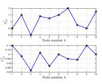
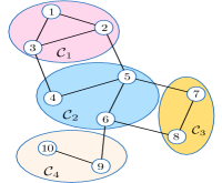
We adopt the same clustered multitask network as [27] in our simulations. As shown in Figure 2, the network consists of 101010 nodes divided into 444 clusters: 𝒞1={1,2,3}subscript𝒞1123{{\mathcal{C}}}_{1}=\{1,2,3\}, 𝒞2={4,5,6}subscript𝒞2456{{\mathcal{C}}}_{2}=\{4,5,6\}, 𝒞3={7,8}subscript𝒞378{{\mathcal{C}}}_{3}=\{7,8\}, 𝒞4={9,10}subscript𝒞4910{{\mathcal{C}}}_{4}=\{9,10\}. The unknown parameter vector 𝒘𝒞isubscriptsuperscript𝒘subscript𝒞𝑖\boldsymbol{w}^{\star}_{{{\mathcal{C}}}_{i}} of each cluster is of size 2×1212\times 1, and has the following form: 𝒘𝒞i=𝒘0+δ𝒘𝒞isubscriptsuperscript𝒘subscript𝒞𝑖subscript𝒘0𝛿subscript𝒘subscript𝒞𝑖\boldsymbol{w}^{\star}_{{{\mathcal{C}}}_{i}}=\boldsymbol{w}_{0}+\delta\boldsymbol{w}_{{{\mathcal{C}}}_{i}} with 𝒘0=[0.5,0.4]subscript𝒘0superscript0.50.4top\boldsymbol{w}_{0}=[0.5,-0.4]^{\top}, δ𝒘𝒞1=[0.0287,0.005]𝛿subscript𝒘subscript𝒞1superscript0.02870.005top\delta\boldsymbol{w}_{{{\mathcal{C}}}_{1}}=[0.0287,-0.005]^{\top}, δ𝒘𝒞2=[0.0234,0.005]𝛿subscript𝒘subscript𝒞2superscript0.02340.005top\delta\boldsymbol{w}_{{{\mathcal{C}}}_{2}}=[0.0234,0.005]^{\top}, δ𝒘𝒞3=[0.0335,0.0029]𝛿subscript𝒘subscript𝒞3superscript0.03350.0029top\delta\boldsymbol{w}_{{{\mathcal{C}}}_{3}}=[-0.0335,0.0029]^{\top}, and δ𝒘𝒞4=[0.0224,0.00347]𝛿subscript𝒘subscript𝒞4superscript0.02240.00347top\delta\boldsymbol{w}_{{{\mathcal{C}}}_{4}}=[0.0224,0.00347]^{\top}. The input and output data at each node k𝑘k are related via the linear regression model: dk(i)=𝒙k(i)𝒘k+zk(i)subscript𝑑𝑘𝑖subscriptsuperscript𝒙top𝑘𝑖superscriptsubscript𝒘𝑘subscript𝑧𝑘𝑖d_{k}(i)=\boldsymbol{x}^{\top}_{k}(i)\boldsymbol{w}_{k}^{\star}+z_{k}(i) where 𝒘k=𝒘𝒞(k)superscriptsubscript𝒘𝑘superscriptsubscript𝒘𝒞𝑘\boldsymbol{w}_{k}^{\star}=\boldsymbol{w}_{{{\mathcal{C}}}(k)}^{\star}. The regressors are zero-mean 2×1212\times 1 random vectors governed by a Gaussian distribution with covariance matrices 𝑹x,k=σx,k2𝑰Lsubscript𝑹𝑥𝑘subscriptsuperscript𝜎2𝑥𝑘subscript𝑰𝐿\boldsymbol{R}_{x,k}=\sigma^{2}_{x,k}\boldsymbol{I}_{L}. The variances σx,k2subscriptsuperscript𝜎2𝑥𝑘\sigma^{2}_{x,k} are shown in Figure 2. The background noises zk(i)subscript𝑧𝑘𝑖z_{k}(i) are independent and identically distributed zero-mean Gaussian random variables, independent of any other signals. The corresponding variances are given in Figure 2.
Refer to caption
Refer to caption
Figure 2: Experimental setup. Left: Network topology. Right: Regression and noise variances.

We considered the Bernoulli asynchronous model described in Appendix A. We set the coefficient aksubscript𝑎𝑘a_{\ell k} in (92) such that ak=|𝒩k𝒞(k)|1subscript𝑎𝑘superscriptsubscript𝒩𝑘𝒞𝑘1a_{\ell k}=|{{\mathcal{N}}}_{k}\cap{{\mathcal{C}}}(k)|^{-1} for all (𝒩k𝒞(k))subscript𝒩𝑘𝒞𝑘\ell\in({{\mathcal{N}}}_{k}\cap{{\mathcal{C}}}(k)), where |𝒩k𝒞(k)|subscript𝒩𝑘𝒞𝑘|{{\mathcal{N}}}_{k}\cap{{\mathcal{C}}}(k)| denotes the cardinality of the set 𝒩k𝒞(k)subscript𝒩𝑘𝒞𝑘{{\mathcal{N}}}_{k}\cap{{\mathcal{C}}}(k). Then we set the regularization factors ρksubscript𝜌𝑘\rho_{k\ell} in (101) as follows. If 𝒩k𝒞(k)subscript𝒩𝑘𝒞𝑘{{\mathcal{N}}}_{k}\setminus{{\mathcal{C}}}(k)\neq\varnothing, ρksubscript𝜌𝑘\rho_{k\ell} was set to ρk=|𝒩k𝒞(k)|1subscript𝜌𝑘superscriptsubscript𝒩𝑘𝒞𝑘1\rho_{k\ell}=|{{\mathcal{N}}}_{k}\setminus{{\mathcal{C}}}(k)|^{-1} for all 𝒩k𝒞(k)subscript𝒩𝑘𝒞𝑘\ell\in{{\mathcal{N}}}_{k}\setminus{{\mathcal{C}}}(k), and to ρk=0subscript𝜌𝑘0\rho_{k\ell}=0 for any other \ell. If 𝒩k𝒞(k)=subscript𝒩𝑘𝒞𝑘{{\mathcal{N}}}_{k}\setminus{{\mathcal{C}}}(k)=\varnothing, these factors were set to ρkk=1subscript𝜌𝑘𝑘1\rho_{kk}=1 and to ρk=0subscript𝜌𝑘0\rho_{k\ell}=0 for all k𝑘\ell\neq k. This usually leads to asymmetrical regularization factors. The parameters of the Bernoulli distribution governing the step-sizes μk(i)subscript𝜇𝑘𝑖\mu_{k}(i) were the same over the network, that is, we set μksubscript𝜇𝑘\mu_{k} in (88) to 0.030.030.03 for all k𝑘k. The regularization strength η𝜂\eta was set to 111. The MSD learning curves were averaged over 100100100 Monte-Carlo runs. The transient MSD curves were obtained with Theorem 3, and the steady-state MSD was estimated with Theorem 4. In Figure 3 (left), we report the network MSD learning curves for 333 different cases:

Case 1: 50%percent5050\% idle: qk=pk=rk=0.5subscript𝑞𝑘subscript𝑝𝑘subscript𝑟𝑘0.5q_{k}=p_{\ell k}=r_{k\ell}=0.5;

Case 2: 30%percent3030\% idle: qk=pk=rk=0.7subscript𝑞𝑘subscript𝑝𝑘subscript𝑟𝑘0.7q_{k}=p_{\ell k}=r_{k\ell}=0.7;

Case 3: no idle nodes: qk=pk=rk=1subscript𝑞𝑘subscript𝑝𝑘subscript𝑟𝑘1q_{k}=p_{\ell k}=r_{k\ell}=1.

We observe that the simulation results match well the theoretical results. Furthermore, the performance of the network is influenced by the probability of occurrence of random events. In Figure 3 (right), the asynchronous algorithm in Case 2 is compared with its synchronous version obtained from (7) by setting μksubscript𝜇𝑘\mu_{k}, aksubscript𝑎𝑘a_{\ell k}, and ρksubscript𝜌𝑘\rho_{k\ell} to the expected values μ¯k=𝔼{μk(i)}subscript¯𝜇𝑘𝔼subscript𝜇𝑘𝑖\bar{\mu}_{k}=\mathbb{E}\{\mu_{k}(i)\}, a¯k=𝔼{ak(i)}subscript¯𝑎𝑘𝔼subscript𝑎𝑘𝑖\bar{a}_{\ell k}=\mathbb{E}\{a_{\ell k}(i)\}, and ρ¯k=𝔼{ρk(i)}subscript¯𝜌𝑘𝔼subscript𝜌𝑘𝑖\bar{\rho}_{k\ell}=\mathbb{E}\{\rho_{k\ell}(i)\}, respectively. Although both algorithms show the same convergence rate, the asynchronous algorithm suffers from degradation in its MSD performance caused by the additional randomness throughout the adaptation process.
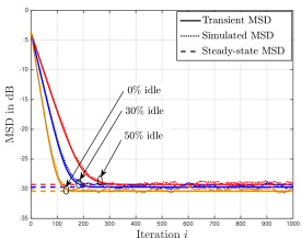
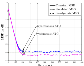
Refer to caption
Refer to caption
Figure 3: Left: Comparison of asynchronous network MSD under 50%percent5050\% idle, 30%percent3030\% idle, and 0%percent00\% idle. Right: Network MSD comparison of asynchronous network under 30%percent3030\% idle and the corresponding synchronous network.

IV-B Multitask learning benefit

In this section we provide an example to show the benefit of multitask learning. We consider a network consisting of N=100𝑁100N=100 nodes grouped into Q=3𝑄3Q=3 clusters such that 𝒞1={1,,70}subscript𝒞1170{{\mathcal{C}}}_{1}=\{1,\ldots,70\}, 𝒞2={71,,90}subscript𝒞27190{{\mathcal{C}}}_{2}=\{71,\ldots,90\}, and 𝒞3={91,,100}subscript𝒞391100{{\mathcal{C}}}_{3}=\{91,\ldots,100\}. The physical connections are defined by the connectivity matrix represented in Figure 4. The inputs 𝒙k(i)subscript𝒙𝑘𝑖\boldsymbol{x}_{k}(i) were zero-mean 21×121121\times 1 random vectors governed by a Gaussian distribution with covariance matrix 𝑹x,k=σx,k2𝑰21subscript𝑹𝑥𝑘subscriptsuperscript𝜎2𝑥𝑘subscript𝑰21\boldsymbol{R}_{x,k}=\sigma^{2}_{x,k}\boldsymbol{I}_{21}, where σx,k2subscriptsuperscript𝜎2𝑥𝑘\sigma^{2}_{x,k} were randomly chosen in the interval [1,1.4]11.4[1,1.4]. The noises zk(i)subscript𝑧𝑘𝑖z_{k}(i) were i.i.d. zero-mean Gaussian random variables, independent of any other signal with variances σz,k2subscriptsuperscript𝜎2𝑧𝑘\sigma^{2}_{z,k} randomly chosen in the interval [0.1,0.15]0.10.15[0.1,0.15]. The 21×121121\times 1 unknown parameter vectors were chosen as: 𝒘𝒞1=𝒘0=[𝟏1×3,𝟎1×3,2𝟏1×3,𝟎1×3,𝟏1×3,𝟎1×3,2𝟏1×3]subscriptsuperscript𝒘subscript𝒞1subscript𝒘0superscriptsubscript113subscript0132subscript113subscript013subscript113subscript0132subscript113top\boldsymbol{w}^{\star}_{{{\mathcal{C}}}_{1}}=\boldsymbol{w}_{0}=[{\boldsymbol{1}}_{1\times 3},{\boldsymbol{0}}_{1\times 3},2\cdot{\boldsymbol{1}}_{1\times 3},{\boldsymbol{0}}_{1\times 3},-{\boldsymbol{1}}_{1\times 3},{\boldsymbol{0}}_{1\times 3},-2\cdot{\boldsymbol{1}}_{1\times 3}]^{\top}, 𝒘𝒞2=𝒘0+δ𝒘subscriptsuperscript𝒘subscript𝒞2subscript𝒘0𝛿𝒘\boldsymbol{w}^{\star}_{{{\mathcal{C}}}_{2}}=\boldsymbol{w}_{0}+\delta\boldsymbol{w}, 𝒘𝒞3=𝒘0δ𝒘subscriptsuperscript𝒘subscript𝒞3subscript𝒘0𝛿𝒘\boldsymbol{w}^{\star}_{{{\mathcal{C}}}_{3}}=\boldsymbol{w}_{0}-\delta\boldsymbol{w} where δ𝒘𝛿𝒘\delta\boldsymbol{w} was randomly generated such that δ𝒘=maxi|[δ𝒘]i|=0.03subscriptnorm𝛿𝒘subscript𝑖subscriptdelimited-[]𝛿𝒘𝑖0.03\|\delta\boldsymbol{w}\|_{\infty}=\max_{i}|[\delta\boldsymbol{w}]_{i}|=0.03.

Refer to caption
Figure 4: Connectivity matrix of the network. The orange, blue, and red elements correspond to links within 𝒞1subscript𝒞1{{\mathcal{C}}}_{1}, 𝒞2subscript𝒞2{{\mathcal{C}}}_{2}, and 𝒞3subscript𝒞3{{\mathcal{C}}}_{3}, respectively. The cyan elements correspond to links between 𝒞1subscript𝒞1{{\mathcal{C}}}_{1} and 𝒞2subscript𝒞2{{\mathcal{C}}}_{2} and the magenta elements correspond to links between 𝒞1subscript𝒞1{{\mathcal{C}}}_{1} and 𝒞3subscript𝒞3{{\mathcal{C}}}_{3}. No links between 𝒞2subscript𝒞2{{\mathcal{C}}}_{2} and 𝒞3subscript𝒞3{{\mathcal{C}}}_{3}.

We considered the Bernoulli asynchronous model. The coefficients {ak}subscript𝑎𝑘\{a_{\ell k}\} and {ρk}subscript𝜌𝑘\{\rho_{k\ell}\} in (92) and (101), respectively, were generated in the same manner as in IV-A. Parameters μksubscript𝜇𝑘\mu_{k} and qksubscript𝑞𝑘q_{k} in (88) were set to μk=1/30subscript𝜇𝑘130\mu_{k}=1/30, qk=0.8subscript𝑞𝑘0.8q_{k}=0.8 for nodes in the first cluster, μk=2/45subscript𝜇𝑘245\mu_{k}=2/45, qk=0.6subscript𝑞𝑘0.6q_{k}=0.6 for nodes in the second cluster, and μk=1/15subscript𝜇𝑘115\mu_{k}=1/15, qk=0.4subscript𝑞𝑘0.4q_{k}=0.4 for nodes in the third cluster. The probabilities {pk}subscript𝑝𝑘\{p_{\ell k}\} in (92) were pk=0.8subscript𝑝𝑘0.8p_{\ell k}=0.8 for links in the first cluster, pk=0.6subscript𝑝𝑘0.6p_{\ell k}=0.6 for links in the second cluster, and pk=0.4subscript𝑝𝑘0.4p_{\ell k}=0.4 for links in the third cluster. The probability that a link connecting two nodes belonging to neighboring clusters drops was 1rk=0.251subscript𝑟𝑘0.251-r_{k\ell}=0.25. The simulated curves were obtained by averaging over 150150150 Monte-Carlo runs.

In Figure 5 (left), we compare two algorithms: the asynchronous diffusion strategy without regularization (obtained from (9) by setting η=0𝜂0\eta=0) and its synchronous counterpart (obtained from (9) by setting η=0𝜂0\eta=0 and replacing μk(i),ak(i)subscript𝜇𝑘𝑖subscript𝑎𝑘𝑖\mu_{k}(i),a_{\ell k}(i) by μ¯k,a¯ksubscript¯𝜇𝑘subscript¯𝑎𝑘\bar{\mu}_{k},\bar{a}_{\ell k}). As shown in this figure, the performance is highly deteriorated in the third cluster and slightly deteriorated in the first cluster because 𝒞3subscript𝒞3{{\mathcal{C}}}_{3} is more susceptible to random events. In Figure 5 (right), we compare two algorithms: the asynchronous diffusion strategy with regularization (obtained from (9) by setting η=2𝜂2\eta=2) and the same synchronous algorithm as in the left plot. As shown in this figure, the cooperation between clusters improves the performance of each cluster so that gaps appearing in the left plot are reduced. In other words, 𝒞2subscript𝒞2{{\mathcal{C}}}_{2} and 𝒞3subscript𝒞3{{\mathcal{C}}}_{3} benefit from the high performance levels achieved by 𝒞1subscript𝒞1{{\mathcal{C}}}_{1}. This can be justified by two arguments: a large number of nodes is employed to collectively estimate 𝒘𝒞1subscriptsuperscript𝒘subscript𝒞1\boldsymbol{w}^{\star}_{{{\mathcal{C}}}_{1}} and the probabilities associated with random events in 𝒞1subscript𝒞1{{\mathcal{C}}}_{1} are small. As a conclusion, when tasks between neighboring clusters are similar, cooperation among clusters improves the learning especially for clusters where asynchronous events occur frequently.
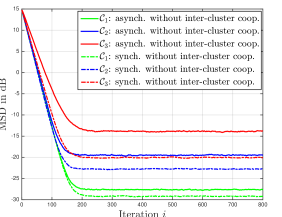
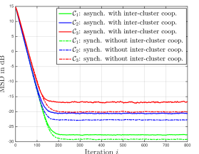
Refer to caption
Refer to caption
Figure 5: Cluster learning curves. Left: Comparison of the asynchronous multitask diffusion LMS (9) without inter-cluster cooperation (η=0)𝜂0(\eta=0) and its synchronous counterpart. Right: Comparison of the asynchronous multitask diffusion LMS (9) with inter-cluster cooperation (η0)𝜂0(\eta\neq 0) and the multitask diffusion LMS (9) without inter-cluster cooperation (η=0)𝜂0(\eta=0).

IV-C Circular arcs localization

In this section, we consider the problem of adaptive surface localization over asynchronous networks. When dealing with a smooth target surface, we can expect that promoting the smoothness of the graph signal will improve the performance of the network [27]. In the following, we consider an arc localization application where the radius of the arc is changing over time, and we illustrate the influence of the random events on the learning behavior and tracking ability of the network.

Let us denote by =[θ0,θ1]subscript𝜃0subscript𝜃1\mathcal{L}=[\theta_{0},\theta_{1}] an arc of circle with radius R𝑅R and subtending an angle θ=θ1θ0𝜃subscript𝜃1subscript𝜃0\theta=\theta_{1}-\theta_{0} with the circle center 𝒘osubscript𝒘𝑜\boldsymbol{w}_{o}. Let us decompose \mathcal{L} into Q𝑄Q sub-arcs qsubscript𝑞\mathcal{L}_{q} with radius R𝑅R and subtending an angle δθmuch-less-than𝛿𝜃\delta\ll\theta with 𝒘osubscript𝒘𝑜\boldsymbol{w}_{o}. In order to estimate the location of \mathcal{L}, and for sufficiently small δ𝛿\delta, it is sufficient to estimate the location of each of these Q𝑄Q sub-arcs by solving a point target localization problem. This can be done by employing a network of N𝑁N nodes, composed of Q𝑄Q clusters, where nodes of each cluster 𝒞qsubscript𝒞𝑞{{\mathcal{C}}}_{q} are interested in locating qsubscript𝑞\mathcal{L}_{q} by estimating a parameter vector 𝒘𝒞qsubscriptsuperscript𝒘subscript𝒞𝑞\boldsymbol{w}^{\star}_{{{\mathcal{C}}}_{q}}. Let us consider node k𝑘k belonging to cluster 𝒞qsubscript𝒞𝑞{{\mathcal{C}}}_{q}. At each time instant i𝑖i, node k𝑘k gets noisy measurements {dk(i),𝒖k(i)}subscript𝑑𝑘𝑖subscript𝒖𝑘𝑖\{d_{k}(i),\boldsymbol{u}_{k}(i)\} that are related via the linear data model [16]:

dk(i)=𝒖k(i)𝒘𝒞q+vk(i),subscript𝑑𝑘𝑖superscriptsubscript𝒖𝑘top𝑖subscriptsuperscript𝒘subscript𝒞𝑞subscript𝑣𝑘𝑖d_{k}(i)=\boldsymbol{u}_{k}^{\top}(i)\boldsymbol{w}^{\star}_{{{\mathcal{C}}}_{q}}+v_{k}(i), (84)

where vk(i)subscript𝑣𝑘𝑖v_{k}(i) is a zero-mean temporally and spatially independent Gaussian noise with variance σv,k2subscriptsuperscript𝜎2𝑣𝑘\sigma^{2}_{v,k}, 𝒖k(i)subscript𝒖𝑘𝑖\boldsymbol{u}_{k}(i) is a noisy measurement of the unit-norm direction vector of 𝒖ksubscript𝒖𝑘\boldsymbol{u}_{k} pointing from agent k𝑘k to the target 𝒘𝒞qsubscriptsuperscript𝒘subscript𝒞𝑞\boldsymbol{w}^{\star}_{{{\mathcal{C}}}_{q}} given by:

𝒖k(i)=𝒖k+αk(i)𝒖k+βk(i)𝒖k,subscript𝒖𝑘𝑖subscript𝒖𝑘subscript𝛼𝑘𝑖superscriptsubscript𝒖𝑘perpendicular-tosubscript𝛽𝑘𝑖subscript𝒖𝑘\boldsymbol{u}_{k}(i)=\boldsymbol{u}_{k}+\alpha_{k}(i)\boldsymbol{u}_{k}^{\perp}+\beta_{k}(i)\boldsymbol{u}_{k}, (85)

with 𝒖ksubscript𝒖𝑘\boldsymbol{u}_{k} given by 𝒖k=(𝒘𝒞q𝒏k)/𝒘𝒞q𝒏ksubscript𝒖𝑘subscriptsuperscript𝒘subscript𝒞𝑞subscript𝒏𝑘normsubscriptsuperscript𝒘subscript𝒞𝑞subscript𝒏𝑘\boldsymbol{u}_{k}=(\boldsymbol{w}^{\star}_{{{\mathcal{C}}}_{q}}-{\boldsymbol{n}}_{k})/\|\boldsymbol{w}^{\star}_{{{\mathcal{C}}}_{q}}-{\boldsymbol{n}}_{k}\| where 𝒏ksubscript𝒏𝑘{\boldsymbol{n}}_{k} is the location vector of node k𝑘k, 𝒖ksuperscriptsubscript𝒖𝑘perpendicular-to\boldsymbol{u}_{k}^{\perp} denoting a unit norm vector that lies in the same space as 𝒖ksubscript𝒖𝑘\boldsymbol{u}_{k} and whose direction is perpendicular to 𝒖ksubscript𝒖𝑘\boldsymbol{u}_{k}. The variables αk(i)subscript𝛼𝑘𝑖\alpha_{k}(i) and βk(i)subscript𝛽𝑘𝑖\beta_{k}(i) are zero-mean independent Gaussian random variables of variances σα,k2subscriptsuperscript𝜎2𝛼𝑘\sigma^{2}_{\alpha,k} and σβ,k2subscriptsuperscript𝜎2𝛽𝑘\sigma^{2}_{\beta,k}, respectively. The amount of perturbation along the parallel direction is assumed to be small compared to the amount of perturbation along the perpendicular direction, that is, σβ,k2σα,k2much-less-thansubscriptsuperscript𝜎2𝛽𝑘subscriptsuperscript𝜎2𝛼𝑘\sigma^{2}_{\beta,k}\ll\sigma^{2}_{\alpha,k}.

To show the effects of randomness at the level of nodes and links, we considered a network of 100100100 nodes grouped into Q=10𝑄10Q=10 clusters, located over arcs of radiuses uniformly distributed between 3R03subscript𝑅03R_{0} and 5R05subscript𝑅05R_{0} given R0subscript𝑅0R_{0}. Angular parameters θ0subscript𝜃0\theta_{0} and θ1subscript𝜃1\theta_{1} were set to 13π/813𝜋813\pi/8 and 15π/815𝜋815\pi/8, respectively. The network topology is shown in Figure 6. The noise variances were set to σv,k2=0.2subscriptsuperscript𝜎2𝑣𝑘0.2\sigma^{2}_{v,k}=0.2, σα,k2=0.05subscriptsuperscript𝜎2𝛼𝑘0.05\sigma^{2}_{\alpha,k}=0.05, and σβ,k2=0.005subscriptsuperscript𝜎2𝛽𝑘0.005\sigma^{2}_{\beta,k}=0.005, for all k𝑘k. We considered a Bernoulli asynchronous model. The coefficients aksubscript𝑎𝑘a_{\ell k} in (92) were set to |𝒩k𝒞(k)|1superscriptsubscript𝒩𝑘𝒞𝑘1|{{\mathcal{N}}}_{k}\cap{{\mathcal{C}}}(k)|^{-1} for intra-cluster links, and to zero for inter-cluster links. The regularization factors ρksubscript𝜌𝑘\rho_{k\ell} in (101) were set to |𝒩k𝒞(k)|1superscriptsubscript𝒩𝑘𝒞𝑘1|{{\mathcal{N}}}_{k}\setminus{{\mathcal{C}}}(k)|^{-1}. The probabilities of success qksubscript𝑞𝑘q_{k}, pksubscript𝑝𝑘p_{\ell k}, and rksubscript𝑟𝑘r_{k\ell} were identically set to 0.50.50.5.

Refer to caption
Figure 6: Network topology consisting of 10 clusters: circles for nodes, solid lines for links, and dashed lines for cluster boundaries.

The MSD learning curves were averaged over 200200200 Monte-Carlo runs. We ran the synchronous and asynchronous multitask algorithms in two different situations. For the first one, we set the regularization strength η𝜂\eta to zero, that is, we did not allow any cooperation between neighboring clusters. In the second one, we set the regularization strength η𝜂\eta to 0.50.50.5. For comparison purposes, we also ran the noncooperative LMS, which was obtained by setting 𝑨(i)=𝑷(i)=𝑰N𝑨𝑖𝑷𝑖subscript𝑰𝑁\boldsymbol{A}(i)=\boldsymbol{P}(i)=\boldsymbol{I}_{N} for all i𝑖i, and the standard diffusion LMS [17]. In both cases, synchronous and asynchronous algorithms were also considered. Each synchronous algorithm was derived from its asynchronous counterpart by making μk(i)subscript𝜇𝑘𝑖\mu_{k}(i), ak(i)subscript𝑎𝑘𝑖a_{\ell k}(i), and ρk(i)subscript𝜌𝑘𝑖\rho_{k\ell}(i) deterministic quantities equal to μ¯ksubscript¯𝜇𝑘\bar{\mu}_{k}, a¯ksubscript¯𝑎𝑘\bar{a}_{\ell k} and ρ¯ksubscript¯𝜌𝑘\bar{\rho}_{k\ell}, respectively. In order to illustrate the tracking ability of the algorithms, we modified the radius R𝑅R of \mathcal{L} every 500500500 iterations such that: for i[0,500]𝑖0500i\in[0,500], R=0.5R0𝑅0.5subscript𝑅0R=0.5R_{0}, for i]500,1000]i\in]500,1000], R=R0𝑅subscript𝑅0R=R_{0}, for i]1000,1500]i\in]1000,1500], R=1.5R0𝑅1.5subscript𝑅0R=1.5R_{0}, and for i]1500,2000]i\in]1500,2000], R=2R0𝑅2subscript𝑅0R=2R_{0}. Note that varying R𝑅R has an effect on the level of similarity between neighboring tasks when characterized by 𝒘𝒞i𝒘𝒞j2superscriptnormsuperscriptsubscript𝒘subscript𝒞𝑖superscriptsubscript𝒘subscript𝒞𝑗2\|\boldsymbol{w}_{{{\mathcal{C}}}_{i}}^{\star}-\boldsymbol{w}_{{{\mathcal{C}}}_{j}}^{\star}\|^{2}, where 𝒞isubscript𝒞𝑖{{\mathcal{C}}}_{i} and 𝒞jsubscript𝒞𝑗{{\mathcal{C}}}_{j} denote two neighboring clusters. Indeed, 𝒘𝒞jsubscriptsuperscript𝒘subscript𝒞𝑗\boldsymbol{w}^{\star}_{{{\mathcal{C}}}_{j}} can be expressed as:

𝒘𝒞j=𝒘o+R(cos(θ0+θQ(j12))sin(θ0+θQ(j12))),j=1,,Q,formulae-sequencesubscriptsuperscript𝒘subscript𝒞𝑗subscript𝒘𝑜𝑅subscript𝜃0𝜃𝑄𝑗12subscript𝜃0𝜃𝑄𝑗12for-all𝑗1𝑄\boldsymbol{w}^{\star}_{{{\mathcal{C}}}_{j}}=\boldsymbol{w}_{o}+R\left(\begin{split}\cos\Big{(}\theta_{0}+\frac{\theta}{Q}\big{(}j-\frac{1}{2}\big{)}\Big{)}\\ \sin\Big{(}\theta_{0}+\frac{\theta}{Q}\big{(}j-\frac{1}{2}\big{)}\Big{)}\end{split}\right),\quad\forall j=1,\ldots,Q, (86)

where θ=θ1θ0𝜃subscript𝜃1subscript𝜃0\theta=\theta_{1}-\theta_{0}. With the topology shown in Fig. 6, we obtain:

𝒘𝒞i𝒘𝒞j2=R2(22cos(θ/Q)).superscriptnormsuperscriptsubscript𝒘subscript𝒞𝑖superscriptsubscript𝒘subscript𝒞𝑗2superscript𝑅222𝜃𝑄\|\boldsymbol{w}_{{{\mathcal{C}}}_{i}}^{\star}-\boldsymbol{w}_{{{\mathcal{C}}}_{j}}^{\star}\|^{2}=R^{2}(2-2\cos(\theta/Q)). (87)

Figure 7 shows that cooperation among clusters improved the network MSD performance and endowed the network with robustness towards asynchronous events. We also observe that the performance of the standard diffusion LMS algorithm deteriorates when the level of similarity between tasks decreases. Figure 8 depicts the estimated arc when R=R0𝑅subscript𝑅0R=R_{0} for the following algorithms in an asynchronous setting: noncooperative LMS obtained by setting 𝑨(i)=𝑷(i)=𝑰N𝑨𝑖𝑷𝑖subscript𝑰𝑁\boldsymbol{A}(i)=\boldsymbol{P}(i)=\boldsymbol{I}_{N} for all i𝑖i, standard diffusion LMS [17], and multitask diffusion LMS (9). In each case, the results were averaged over 150 Monte-Carlo runs and over 50 samples after convergence. The multitask diffusion algorithm outperformed the non cooperative LMS and the standard diffusion. The standard diffusion was not able to estimate the location of the target since it is a single task algorithm. It is shown in [29] that standard diffusion LMS converges to a Pareto optimal solution when it is applied to multitask problems.
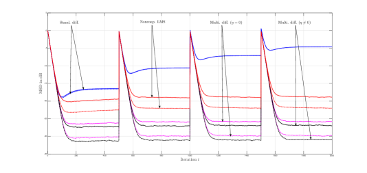
Refer to caption
Figure 7: Network topology consisting of 10 clusters. Network MSD learning curves in a non-stationary environment: comparison of the multitask diffusion LMS with (namely, η>0𝜂0\eta>0) and without (namely, η=0𝜂0\eta=0) inter-cluster cooperation, the standard diffusion LMS [17] and the non-cooperative LMS. The dotted lines are for synchronous networks and the solid lines are for asynchronous networks.
Refer to caption
Figure 8: Target estimation results (R=R0=2𝑅subscript𝑅02R=R_{0}=2) over asynchronous network: black cross sign for multitask diffusion (9), red asterisk sign for non-cooperative, and blue circle sign for standard diffusion [17].

Finally, in order to show the effects of the number of clusters (or tasks) on the performance of the network, we considered 2 additional experimental setups. In the first one represented in Figure 9 (left), the number of tasks was set to 555, that is, the arc \mathcal{L} was decomposed into 5 sub-arcs. In the second one depicted in Figure 9 (right), the number of clusters was set to 15. Except for these changes, we considered the same experimental setup as before. Every 500500500 time steps, the radius R𝑅R of the arc was modified as before in order to decrease the similarity level between tasks. The learning curves of the algorithms considered in Figure 7 are reported in Figure 10. As expected, it can be observed that the larger the number of clusters is, the more efficient the collaboration between clusters becomes. The benefits of inter-cluster cooperation decreases when the number of clusters becomes small.
Refer to caption
Refer to caption
Figure 9: Network topology: circles for nodes, solid lines for links, and dashed lines for cluster boundaries. Left: network consisting of 5 clusters. Right: network consisting of 15 clusters.
Refer to caption
Refer to caption
Figure 10: Network MSD learning curves in a non-stationary environment: comparison of the same algorithms considered in Figure 7. The dotted lines are for synchronous networks and the solid lines are for asynchronous networks. Top: network consisting of 555 clusters. Down: Network consisting of 151515 clusters.

V Conclusion and perspectives

In this paper, we considered multitask problems where networks are able to handle situations beyond the case where the nodes estimate a unique parameter vector over the network. We introduced a general model for asynchronous behavior with random step-sizes, combination coefficients, and co-regularization factors. We then carried out a convergence analysis of the asynchronous multitask algorithm in the mean and mean-square-error sense, and we derived conditions for convergence. Several open problems still have to be solved for specific applications. For instance, it would be interesting to investigate how nodes can autonomously adjust co-regularization factors between neighboring clusters in order to optimize the learning performance. It would also be advantageous to consider alternative co-regularizers in order to promote properties such as sparsity or block sparsity, and to analyze the convergence behavior of the resulting algorithms.

Appendix A The Bernoulli model

In this model, the step-sizes {μk(i)}subscript𝜇𝑘𝑖\{\mu_{k}(i)\} are distributed as follows:

μk(i)={μk,with probability qk0,with probability 1qksubscript𝜇𝑘𝑖casessubscript𝜇𝑘with probability subscript𝑞𝑘0with probability 1subscript𝑞𝑘\mu_{k}(i)=\left\{\begin{array}[]{ll}\mu_{k},&\text{with probability }q_{k}\\ 0,&\text{with probability }1-q_{k}\\ \end{array}\right. (88)

where μksubscript𝜇𝑘\mu_{k} is a fixed value. This probability distribution allows us to model random “on-off” behavior by each agent k𝑘k due to power saving strategies or random agent failures. We assume that the step-sizes μk(i)subscript𝜇𝑘𝑖\mu_{k}(i) are spatially uncorrelated for different k𝑘k. At each iteration i𝑖i, the mean of the step-size μk(i)subscript𝜇𝑘𝑖\mu_{k}(i) is μ¯k=μkqksubscript¯𝜇𝑘subscript𝜇𝑘subscript𝑞𝑘\bar{\mu}_{k}=\mu_{k}q_{k}, and the covariance between μk(i)subscript𝜇𝑘𝑖\mu_{k}(i) and μ(i)subscript𝜇𝑖\mu_{\ell}(i) is:

cμ,k,subscript𝑐𝜇𝑘\displaystyle c_{\mu,k,\ell} 𝔼{(μk(i)μ¯k)(μ(i)μ¯)}absent𝔼subscript𝜇𝑘𝑖subscript¯𝜇𝑘subscript𝜇𝑖subscript¯𝜇\displaystyle\triangleq\mathbb{E}\{(\mu_{k}(i)-\bar{\mu}_{k})(\mu_{\ell}(i)-\bar{\mu}_{\ell})\}
={μk2qk(1qk),if =k0,otherwise.absentcasessuperscriptsubscript𝜇𝑘2subscript𝑞𝑘1subscript𝑞𝑘if 𝑘missing-subexpression0otherwise.missing-subexpression\displaystyle=\left\{\begin{array}[]{lr}\mu_{k}^{2}q_{k}(1-q_{k}),\quad\text{if }\ell=k\\ 0,\quad\quad\quad\quad\quad\quad\text{otherwise.}\\ \end{array}\right. (91)

Furthermore, combination weights {ak(i)}subscript𝑎𝑘𝑖\{a_{\ell k}(i)\} are distributed as follows:

ak(i)={ak,with probability pk0,with probability 1pksubscript𝑎𝑘𝑖casessubscript𝑎𝑘with probability subscript𝑝𝑘missing-subexpression0with probability 1subscript𝑝𝑘missing-subexpressiona_{\ell k}(i)=\left\{\begin{array}[]{lll}a_{\ell k},&\text{with probability }p_{\ell k}\\ 0,&\text{with probability }1-p_{\ell k}\\ \end{array}\right. (92)

for any 𝒩k(i)𝒞(k)subscriptsuperscript𝒩𝑘𝑖𝒞𝑘\ell\in{{\mathcal{N}}}^{-}_{k}(i)\cap{{\mathcal{C}}}(k), where 0<ak<10subscript𝑎𝑘10<a_{\ell k}<1 a fixed coefficient. The coefficients {ak(i)}subscript𝑎𝑘𝑖\{a_{\ell k}(i)\} are spatially uncorrelated for different \ell and k𝑘k. Node k𝑘k adjusts its own combination coefficient to ensure that the sum of its neighboring coefficients is equal to one as follows:

akk(i)=1𝒩k(i)𝒞(k)ak(i)0.subscript𝑎𝑘𝑘𝑖1subscriptsubscriptsuperscript𝒩𝑘𝑖𝒞𝑘subscript𝑎𝑘𝑖0a_{kk}(i)=1-\sum_{\ell\in{{\mathcal{N}}}^{-}_{k}(i)\cap{{\mathcal{C}}}(k)}a_{\ell k}(i)\,\geq 0. (93)

The probability distribution (92) allows us to model a random “on-off” status for links within clusters at time i𝑖i due to communication cost saving strategies or random link failures. With this model, we are giving the opportunity to each agent k𝑘k to randomly choose a subset of neighbors that belong to its cluster to perform the combination step. At each iteration i𝑖i, the mean of the coefficient ak(i)subscript𝑎𝑘𝑖a_{\ell k}(i) is given by:

a¯k={akpk,if𝒩k𝒞(k)1𝒩k𝒞(k)akpk,if=k0,otherwise.subscript¯𝑎𝑘casessubscript𝑎𝑘subscript𝑝𝑘ifsubscriptsuperscript𝒩𝑘𝒞𝑘1subscriptsuperscriptsubscript𝒩𝑘𝒞𝑘subscript𝑎𝑘subscript𝑝𝑘if𝑘0otherwise\bar{a}_{\ell k}=\left\{\begin{array}[]{ll}a_{\ell k}p_{\ell k},&\text{if}\quad\ell\in{{\mathcal{N}}}^{-}_{k}\cap{{\mathcal{C}}}(k)\\ 1-\sum\limits_{\ell\in{{\mathcal{N}}}_{k}^{-}\cap{{\mathcal{C}}}(k)}a_{\ell k}p_{\ell k},&\text{if}\quad\ell=k\\ 0,&\text{otherwise}.\end{array}\right. (94)

and the covariance between ak(i)subscript𝑎𝑘𝑖a_{\ell k}(i) and anm(i)subscript𝑎𝑛𝑚𝑖a_{nm}(i) equals [42]:

ca,k,nm=𝔼{(ak(i)a¯k)(anm(i)a¯nm)}subscript𝑐𝑎𝑘𝑛𝑚𝔼subscript𝑎𝑘𝑖subscript¯𝑎𝑘subscript𝑎𝑛𝑚𝑖subscript¯𝑎𝑛𝑚\displaystyle c_{a,\ell k,nm}=\mathbb{E}\{(a_{\ell k}(i)-\overline{a}_{\ell k})(a_{nm}(i)-\overline{a}_{nm})\}
={ca,k,k,if k=m,=n,𝒩k𝒞(k)ca,k,k,if k=m=n,𝒩k𝒞(k)ca,nk,nk,if k=m=,n𝒩k𝒞(k)j𝒩k𝒞(k)ca,jk,jk,if k=m==n0,otherwise.absentcasessubscript𝑐𝑎𝑘𝑘formulae-sequenceif 𝑘𝑚formulae-sequence𝑛subscriptsuperscript𝒩𝑘𝒞𝑘subscript𝑐𝑎𝑘𝑘formulae-sequenceif 𝑘𝑚𝑛subscriptsuperscript𝒩𝑘𝒞𝑘subscript𝑐𝑎𝑛𝑘𝑛𝑘formulae-sequenceif 𝑘𝑚𝑛subscriptsuperscript𝒩𝑘𝒞𝑘subscript𝑗subscriptsuperscript𝒩𝑘𝒞𝑘subscript𝑐𝑎𝑗𝑘𝑗𝑘if 𝑘𝑚𝑛0otherwise.\displaystyle=\left\{\begin{array}[]{ll}c_{a,\ell k,\ell k},&\text{if }k=m,\ell=n,\ell\in{{\mathcal{N}}}^{-}_{k}\cap{{\mathcal{C}}}(k)\\ -c_{a,\ell k,\ell k},&\text{if }k=m=n,\ell\in{{\mathcal{N}}}^{-}_{k}\cap{{\mathcal{C}}}(k)\\ -c_{a,nk,nk},&\text{if }k=m=\ell,n\in{{\mathcal{N}}}^{-}_{k}\cap{{\mathcal{C}}}(k)\\ \sum\limits_{j\in{{\mathcal{N}}}^{-}_{k}\cap{{\mathcal{C}}}(k)}c_{a,jk,jk},&\text{if }k=m=\ell=n\\ 0,&\text{otherwise.}\end{array}\right. (100)

where ca,k,k=ak2pk(1pk)subscript𝑐𝑎𝑘𝑘superscriptsubscript𝑎𝑘2subscript𝑝𝑘1subscript𝑝𝑘c_{a,\ell k,\ell k}=a_{\ell k}^{2}p_{\ell k}(1-p_{\ell k}).

Finally, the regularization factors {ρk(i)}subscript𝜌𝑘𝑖\{\rho_{k\ell}(i)\} are distributed as follows:

ρk(i)={ρk,with probability rk0,with probability 1rksubscript𝜌𝑘𝑖casessubscript𝜌𝑘with probability subscript𝑟𝑘0with probability 1subscript𝑟𝑘\rho_{k\ell}(i)=\left\{\begin{array}[]{ll}\rho_{k\ell},&\text{with probability }r_{k\ell}\\ 0,&\text{with probability }1-r_{k\ell}\\ \end{array}\right. (101)

for any 𝒩k(i)𝒞(k)subscript𝒩𝑘𝑖𝒞𝑘\ell\in{{\mathcal{N}}}_{k}(i)\setminus{{\mathcal{C}}}(k), where 0<ρk<10subscript𝜌𝑘10<\rho_{k\ell}<1 is a fixed regularization factor. The factors {ρk(i)}subscript𝜌𝑘𝑖\{\rho_{k\ell}(i)\} are spatially uncorrelated for k𝑘k\neq\ell. At each iteration i𝑖i, in order to get a right stochastic matrix 𝑷(i)𝑷𝑖\boldsymbol{P}(i), node k𝑘k adjusts its regularization factor as follows:

ρkk(i)=1𝒩k(i)𝒞(k)ρk(i)0.subscript𝜌𝑘𝑘𝑖1subscriptsubscript𝒩𝑘𝑖𝒞𝑘subscript𝜌𝑘𝑖0\rho_{kk}(i)=1-\sum_{\ell\in{{\mathcal{N}}}_{k}(i)\setminus{{\mathcal{C}}}(k)}\rho_{k\ell}(i)\,\geq 0. (102)

The probability distribution (101) allows each agent k𝑘k to randomly select a subset of neighbors that do not belong to its cluster and introduce co-regularization in the estimation process. This behavior can also be interpreted as resulting from link random failures between neighboring clusters: at every time instant i𝑖i, the communication link from agent \ell to agent k𝑘k drops with probability 1rk1subscript𝑟𝑘1-r_{k\ell}. The mean of ρk(i)subscript𝜌𝑘𝑖\rho_{k\ell}(i) is given:

ρ¯k={ρkrk,if 𝒩k𝒞(k)1𝒩k𝒞(k)ρkrk,if=k0,otherwise,subscript¯𝜌𝑘casessubscript𝜌𝑘subscript𝑟𝑘if subscript𝒩𝑘𝒞𝑘1subscriptsubscript𝒩𝑘𝒞𝑘subscript𝜌𝑘subscript𝑟𝑘if𝑘0otherwise\overline{\rho}_{k\ell}=\left\{\begin{array}[]{ll}\rho_{k\ell}r_{k\ell},&\text{if }\ell\in{{\mathcal{N}}}_{k}\setminus{{\mathcal{C}}}(k)\\ 1-\sum\limits_{\ell\in{{\mathcal{N}}}_{k}\setminus{{\mathcal{C}}}(k)}\rho_{k\ell}r_{k\ell},&\text{if}\quad\ell=k\\ 0,&\text{otherwise},\end{array}\right. (103)

and the covariance between ρk(i)subscript𝜌𝑘𝑖\rho_{k\ell}(i) and ρmn(i)subscript𝜌𝑚𝑛𝑖\rho_{mn}(i) is:

cρ,k,mn=𝔼{(ρk(i)ρ¯k)(ρmn(i)ρ¯mn)}subscript𝑐𝜌𝑘𝑚𝑛𝔼subscript𝜌𝑘𝑖subscript¯𝜌𝑘subscript𝜌𝑚𝑛𝑖subscript¯𝜌𝑚𝑛\displaystyle c_{\rho,k\ell,mn}=\mathbb{E}\{(\rho_{k\ell}(i)-\overline{\rho}_{k\ell})(\rho_{mn}(i)-\overline{\rho}_{mn})\}
={cρ,k,k,if k=m,=n,𝒩k𝒞(k)cρ,k,k,if k=m=n,𝒩k𝒞(k)cρ,kn,kn,if k=m=,n𝒩k𝒞(k)j𝒩k𝒞(k)cρ,kj,kj,if k=m==n0,otherwiseabsentcasessubscript𝑐𝜌𝑘𝑘formulae-sequenceif 𝑘𝑚formulae-sequence𝑛subscript𝒩𝑘𝒞𝑘subscript𝑐𝜌𝑘𝑘formulae-sequenceif 𝑘𝑚𝑛subscript𝒩𝑘𝒞𝑘subscript𝑐𝜌𝑘𝑛𝑘𝑛formulae-sequenceif 𝑘𝑚𝑛subscript𝒩𝑘𝒞𝑘subscript𝑗subscript𝒩𝑘𝒞𝑘subscript𝑐𝜌𝑘𝑗𝑘𝑗if 𝑘𝑚𝑛0otherwise\displaystyle=\left\{\begin{array}[]{ll}c_{\rho,k\ell,k\ell},&\text{if }k=m,\ell=n,\ell\in{{\mathcal{N}}}_{k}\setminus{{\mathcal{C}}}(k)\\ -c_{\rho,k\ell,k\ell},&\text{if }k=m=n,\ell\in{{\mathcal{N}}}_{k}\setminus{{\mathcal{C}}}(k)\\ -c_{\rho,kn,kn},&\text{if }k=m=\ell,n\in{{\mathcal{N}}}_{k}\setminus{{\mathcal{C}}}(k)\\ \sum\limits_{j\in{{\mathcal{N}}}_{k}\setminus{{\mathcal{C}}}(k)}c_{\rho,kj,kj},&\text{if }k=m=\ell=n\\ 0,&\text{otherwise}\end{array}\right. (109)

where cρ,k,k=ρk2rk(1rk)subscript𝑐𝜌𝑘𝑘superscriptsubscript𝜌𝑘2subscript𝑟𝑘1subscript𝑟𝑘c_{\rho,k\ell,k\ell}=\rho_{k\ell}^{2}r_{k\ell}(1-r_{k\ell}).

Appendix B Stability of 𝓕𝓕{\boldsymbol{\mathcal{F}}}

Recall from (III-B) that

𝓕𝓐 I[\displaystyle{\boldsymbol{\mathcal{F}}}\approx{\boldsymbol{\mathcal{A}}}_{\text{\,I}}^{\top}[ 𝑰(NL)2𝑰NLb𝓜(𝓡x+η𝓠)subscript𝑰superscript𝑁𝐿2limit-fromsubscripttensor-product𝑏subscript𝑰𝑁𝐿𝓜subscript𝓡𝑥𝜂𝓠\displaystyle\boldsymbol{I}_{(NL)^{2}}-\boldsymbol{I}_{NL}\otimes_{b}{\boldsymbol{\mathcal{M}}}({\boldsymbol{\mathcal{R}}}_{x}+\eta{\boldsymbol{\mathcal{Q}}})-
𝓜(𝓡x+η𝓠)b𝑰NL].\displaystyle{\boldsymbol{\mathcal{M}}}({\boldsymbol{\mathcal{R}}}_{x}+\eta{\boldsymbol{\mathcal{Q}}})\otimes_{b}\boldsymbol{I}_{NL}]. (110)

We now upper-bound the spectral radius of 𝓕𝓕{\boldsymbol{\mathcal{F}}} in order to derive a sufficient condition for mean-square stability of the algorithm. We can write:

ρ(𝓕)𝓐 Ib,\displaystyle\rho({\boldsymbol{\mathcal{F}}})\leq\|{\boldsymbol{\mathcal{A}}}_{\text{\,I}}^{\top}\|_{b,\infty}\cdot\| 𝑰(NL)2𝑰NLb𝓜(𝓡x+η𝓠)subscript𝑰superscript𝑁𝐿2limit-fromsubscripttensor-product𝑏subscript𝑰𝑁𝐿𝓜subscript𝓡𝑥𝜂𝓠\displaystyle\boldsymbol{I}_{(NL)^{2}}-\boldsymbol{I}_{NL}\otimes_{b}{\boldsymbol{\mathcal{M}}}({\boldsymbol{\mathcal{R}}}_{x}+\eta{\boldsymbol{\mathcal{Q}}})-
𝓜(𝓡x+η𝓠)b𝑰NLb,evaluated-atsubscripttensor-product𝑏𝓜subscript𝓡𝑥𝜂𝓠subscript𝑰𝑁𝐿𝑏\displaystyle{\boldsymbol{\mathcal{M}}}({\boldsymbol{\mathcal{R}}}_{x}+\eta{\boldsymbol{\mathcal{Q}}})\otimes_{b}\boldsymbol{I}_{NL}\|_{b,\infty} (111)

Since the matrix 𝓐 Isubscript𝓐 I{\boldsymbol{\mathcal{A}}}_{\text{\,I}} is a block left-stochastic matrix, we know that 𝓐 Ib,=1subscriptnormsuperscriptsubscript𝓐 Itop𝑏1\|{\boldsymbol{\mathcal{A}}}_{\text{\,I}}^{\top}\|_{b,\infty}=1. Using (42) and the triangular inequality, we have:

ρ(𝓕)𝜌𝓕\displaystyle\rho({\boldsymbol{\mathcal{F}}}) 𝑰(NL)2𝑰NLb𝓜(𝓡x+η𝑰NL)\displaystyle\leq\|\boldsymbol{I}_{(NL)^{2}}-\boldsymbol{I}_{NL}\otimes_{b}{\boldsymbol{\mathcal{M}}}({\boldsymbol{\mathcal{R}}}_{x}+\eta\boldsymbol{I}_{NL})-
𝓜(𝓡x+η𝑰NL)b𝑰NLb,evaluated-atsubscripttensor-product𝑏𝓜subscript𝓡𝑥𝜂subscript𝑰𝑁𝐿subscript𝑰𝑁𝐿𝑏\displaystyle\quad\quad\quad\quad\quad{\boldsymbol{\mathcal{M}}}({\boldsymbol{\mathcal{R}}}_{x}+\eta\boldsymbol{I}_{NL})\otimes_{b}\boldsymbol{I}_{NL}\|_{b,\infty}
+η𝑰NLb𝓜𝓟b,+η𝓜𝓟b𝑰NLb,.𝜂subscriptnormsubscripttensor-product𝑏subscript𝑰𝑁𝐿𝓜𝓟𝑏𝜂subscriptnormsubscripttensor-product𝑏𝓜𝓟subscript𝑰𝑁𝐿𝑏\displaystyle+\eta\|\boldsymbol{I}_{NL}\otimes_{b}{\boldsymbol{\mathcal{MP}}}\|_{b,\infty}+\eta\|{\boldsymbol{\mathcal{M}}}{\boldsymbol{\mathcal{P}}}\otimes_{b}\boldsymbol{I}_{NL}\|_{b,\infty}. (112)

Consider the second term on the RHS of (B). We know that

𝑰NLb𝓜𝓟subscripttensor-product𝑏subscript𝑰𝑁𝐿𝓜𝓟\displaystyle\boldsymbol{I}_{NL}\otimes_{b}{\boldsymbol{\mathcal{MP}}} =(54)(𝑰NLb𝓜)(𝑰NLb𝓟)italic-(54italic-)subscripttensor-product𝑏subscript𝑰𝑁𝐿𝓜subscripttensor-product𝑏subscript𝑰𝑁𝐿𝓟\displaystyle\overset{\eqref{property 3}}{=}(\boldsymbol{I}_{NL}\otimes_{b}{\boldsymbol{\mathcal{M}}})(\boldsymbol{I}_{NL}\otimes_{b}{\boldsymbol{\mathcal{P}}})
=(55)((𝑰N𝑴¯)𝑰L2)((𝑰N𝑷¯)𝑰L2).italic-(55italic-)tensor-producttensor-productsubscript𝑰𝑁¯𝑴subscript𝑰superscript𝐿2tensor-producttensor-productsubscript𝑰𝑁¯𝑷subscript𝑰superscript𝐿2\displaystyle\overset{\eqref{property 4}}{=}\Big{(}(\boldsymbol{I}_{N}\otimes\overline{\boldsymbol{M}})\otimes\boldsymbol{I}_{L^{2}}\Big{)}\Big{(}(\boldsymbol{I}_{N}\otimes\overline{\boldsymbol{P}})\otimes\boldsymbol{I}_{L^{2}}\Big{)}. (113)

Since ((𝑰N𝑷¯)𝑰L2)tensor-producttensor-productsubscript𝑰𝑁¯𝑷subscript𝑰superscript𝐿2\Big{(}(\boldsymbol{I}_{N}\otimes\overline{\boldsymbol{P}})\otimes\boldsymbol{I}_{L^{2}}\Big{)} is a block right-stochastic matrix and ((𝑰N𝑴¯)𝑰L2)tensor-producttensor-productsubscript𝑰𝑁¯𝑴subscript𝑰superscript𝐿2\Big{(}(\boldsymbol{I}_{N}\otimes\overline{\boldsymbol{M}})\otimes\boldsymbol{I}_{L^{2}}\Big{)} is an N2×N2superscript𝑁2superscript𝑁2N^{2}\times N^{2} block diagonal matrix with each block of the form μ¯k𝑰L2subscript¯𝜇𝑘subscript𝑰superscript𝐿2\bar{\mu}_{k}\boldsymbol{I}_{L^{2}} (k=1,,N𝑘1𝑁k=1,\ldots,N), we obtain:

𝑰NLb𝓜𝓟b,subscriptnormsubscripttensor-product𝑏subscript𝑰𝑁𝐿𝓜𝓟𝑏\displaystyle\|\boldsymbol{I}_{NL}\otimes_{b}{\boldsymbol{\mathcal{MP}}}\|_{b,\infty}
(𝑰N𝑴¯)𝑰L2b,(𝑰N𝑷¯)𝑰L2b,absentsubscriptnormtensor-producttensor-productsubscript𝑰𝑁¯𝑴subscript𝑰superscript𝐿2𝑏subscriptnormtensor-producttensor-productsubscript𝑰𝑁¯𝑷subscript𝑰superscript𝐿2𝑏\displaystyle\leq\|(\boldsymbol{I}_{N}\otimes\overline{\boldsymbol{M}})\otimes\boldsymbol{I}_{L^{2}}\|_{b,\infty}\cdot\|(\boldsymbol{I}_{N}\otimes\overline{\boldsymbol{P}})\otimes\boldsymbol{I}_{L^{2}}\|_{b,\infty}
=max1kNμ¯kabsentsubscript1𝑘𝑁subscript¯𝜇𝑘\displaystyle=\max_{1\leq k\leq N}\overline{\mu}_{k} (114)

Following the same steps for the third term on the RHS of (B), we have:

𝓜𝓟b𝑰NLb,max1kNμ¯k.subscriptnormsubscripttensor-product𝑏𝓜𝓟subscript𝑰𝑁𝐿𝑏subscript1𝑘𝑁subscript¯𝜇𝑘\|{\boldsymbol{\mathcal{MP}}}\otimes_{b}\boldsymbol{I}_{NL}\|_{b,\infty}\leq\max_{1\leq k\leq N}\overline{\mu}_{k}. (115)

The matrix [𝑰(NL)2𝑰NLb𝓜(𝓡x+η𝑰NL)𝓜(𝓡x+η𝑰NL)b𝑰NL]delimited-[]subscript𝑰superscript𝑁𝐿2subscripttensor-product𝑏subscript𝑰𝑁𝐿𝓜subscript𝓡𝑥𝜂subscript𝑰𝑁𝐿subscripttensor-product𝑏𝓜subscript𝓡𝑥𝜂subscript𝑰𝑁𝐿subscript𝑰𝑁𝐿\big{[}\boldsymbol{I}_{(NL)^{2}}-\boldsymbol{I}_{NL}\otimes_{b}{\boldsymbol{\mathcal{M}}}({\boldsymbol{\mathcal{R}}}_{x}+\eta\boldsymbol{I}_{NL})-{\boldsymbol{\mathcal{M}}}({\boldsymbol{\mathcal{R}}}_{x}+\eta\boldsymbol{I}_{NL})\otimes_{b}\boldsymbol{I}_{NL}\big{]} in the first term on the RHS of (B) is an N2×N2superscript𝑁2superscript𝑁2N^{2}\times N^{2} block diagonal matrix. The m𝑚m-th block on the diagonal (where m=(1)N+k𝑚1𝑁𝑘m=(\ell-1)N+k for k,=1,,Nformulae-sequence𝑘1𝑁k,\ell=1,\ldots,N) is of size L2×L2superscript𝐿2superscript𝐿2L^{2}\times L^{2}, symmetric, and has the following form:

𝑰L2𝑰Lμ¯k(𝑹x,k+η𝑰L)μ¯(𝑹x,+η𝑰L)𝑰Lsubscript𝑰superscript𝐿2tensor-productsubscript𝑰𝐿subscript¯𝜇𝑘subscript𝑹𝑥𝑘𝜂subscript𝑰𝐿tensor-productsubscript¯𝜇subscript𝑹𝑥𝜂subscript𝑰𝐿subscript𝑰𝐿\displaystyle\boldsymbol{I}_{L^{2}}-\boldsymbol{I}_{L}\otimes\bar{\mu}_{k}(\boldsymbol{R}_{x,k}+\eta\boldsymbol{I}_{L})-\bar{\mu}_{\ell}(\boldsymbol{R}_{x,\ell}+\eta\boldsymbol{I}_{L})\otimes\boldsymbol{I}_{L}
=(μ¯𝑹x,ημ¯𝑰L)𝑰L+𝑰L(𝑰Lμ¯k𝑹x,kημ¯k𝑰L)absenttensor-productsubscript¯𝜇subscript𝑹𝑥𝜂subscript¯𝜇subscript𝑰𝐿subscript𝑰𝐿tensor-productsubscript𝑰𝐿subscript𝑰𝐿subscript¯𝜇𝑘subscript𝑹𝑥𝑘𝜂subscript¯𝜇𝑘subscript𝑰𝐿\displaystyle=(-\bar{\mu}_{\ell}\boldsymbol{R}_{x,\ell}-\eta\bar{\mu}_{\ell}\boldsymbol{I}_{L})\otimes\boldsymbol{I}_{L}+\boldsymbol{I}_{L}\otimes(\boldsymbol{I}_{L}-\bar{\mu}_{k}\boldsymbol{R}_{x,k}-\eta\bar{\mu}_{k}\boldsymbol{I}_{L}) (116)

Before proceeding, let us recall the Kronecker sum operator, denoted by direct-sum\oplus. If 𝑨𝑨\boldsymbol{A} and 𝑩𝑩\boldsymbol{B} are two matrices of dimension L×L𝐿𝐿L\times L each, then

𝑨𝑩𝑨𝑰L+𝑰L𝑩.direct-sum𝑨𝑩tensor-product𝑨subscript𝑰𝐿tensor-productsubscript𝑰𝐿𝑩\boldsymbol{A}\oplus\boldsymbol{B}\triangleq\boldsymbol{A}\otimes\boldsymbol{I}_{L}+\boldsymbol{I}_{L}\otimes\boldsymbol{B}. (117)

Let λk{}subscript𝜆𝑘\lambda_{k}\{\cdot\} denote the k𝑘k-th eigenvalue of its matrix argument. Then, the eigenvalues of 𝑨𝑩direct-sum𝑨𝑩\boldsymbol{A}\oplus\boldsymbol{B} are of the form λi{𝑨}+λj{𝑩}subscript𝜆𝑖𝑨subscript𝜆𝑗𝑩\lambda_{i}\{\boldsymbol{A}\}+\lambda_{j}\{\boldsymbol{B}\} for i𝑖i, j=1,,L𝑗1𝐿j=1,\ldots,L [50]. Note that the RHS of equation (B) can be written as

(μ¯𝑹x,ημ¯𝑰L)(𝑰Lμ¯k𝑹x,kημ¯k𝑰L)direct-sumsubscript¯𝜇subscript𝑹𝑥𝜂subscript¯𝜇subscript𝑰𝐿subscript𝑰𝐿subscript¯𝜇𝑘subscript𝑹𝑥𝑘𝜂subscript¯𝜇𝑘subscript𝑰𝐿(-\bar{\mu}_{\ell}\boldsymbol{R}_{x,\ell}-\eta\bar{\mu}_{\ell}\boldsymbol{I}_{L})\oplus(\boldsymbol{I}_{L}-\bar{\mu}_{k}\boldsymbol{R}_{x,k}-\eta\bar{\mu}_{k}\boldsymbol{I}_{L}) (118)

and its eigenvalues are therefore of the form:

1ημ¯kμ¯kλj{𝑹x,k}ημ¯μ¯λi{𝑹x,}1𝜂subscript¯𝜇𝑘subscript¯𝜇𝑘subscript𝜆𝑗subscript𝑹𝑥𝑘𝜂subscript¯𝜇subscript¯𝜇subscript𝜆𝑖subscript𝑹𝑥1-\eta\bar{\mu}_{k}-\bar{\mu}_{k}\lambda_{j}\{\boldsymbol{R}_{x,k}\}-\eta\bar{\mu}_{\ell}-\bar{\mu}_{\ell}\lambda_{i}\{\boldsymbol{R}_{x,\ell}\} (119)

for i𝑖i, j=1,,L𝑗1𝐿j=1,\ldots,L and k𝑘k, =1,,N1𝑁\ell=1,\ldots,N. In order to simplify the mean-square stability condition, we assume that the first order moment of the step-sizes is the same for all nodes. Using the fact that the block maximum norm of a block diagonal Hermitian matrix is equal to the largest spectral radius of its block entries [16], we get:

𝑰(NL)2𝑰NLb𝓜(𝓡x+η𝑰NL)\displaystyle\|\boldsymbol{I}_{(NL)^{2}}-\boldsymbol{I}_{NL}\otimes_{b}{\boldsymbol{\mathcal{M}}}({\boldsymbol{\mathcal{R}}}_{x}+\eta\boldsymbol{I}_{NL})-
𝓜(𝓡x+η𝑰NL)b𝑰NLb,evaluated-atsubscripttensor-product𝑏𝓜subscript𝓡𝑥𝜂subscript𝑰𝑁𝐿subscript𝑰𝑁𝐿𝑏\displaystyle\quad\quad\quad\quad\quad\quad{\boldsymbol{\mathcal{M}}}({\boldsymbol{\mathcal{R}}}_{x}+\eta\boldsymbol{I}_{NL})\otimes_{b}\boldsymbol{I}_{NL}\|_{b,\infty}
=max1k,N(max1i,jL|12ημ¯μ¯(λj{𝑹x,k}+λi{𝑹x,})|)absentsubscriptformulae-sequence1𝑘𝑁subscriptformulae-sequence1𝑖𝑗𝐿12𝜂¯𝜇¯𝜇subscript𝜆𝑗subscript𝑹𝑥𝑘subscript𝜆𝑖subscript𝑹𝑥\displaystyle=\max_{1\leq k,\ell\leq N}\Big{(}\max_{1\leq i,j\leq L}|1-2\eta\bar{\mu}-\bar{\mu}(\lambda_{j}\{\boldsymbol{R}_{x,k}\}+\lambda_{i}\{\boldsymbol{R}_{x,\ell}\})|\,\Big{)}
=max1k,N(max1i,jL{12ημ¯μ¯(λj{𝑹x,k}+λi{𝑹x,}),\displaystyle=\max_{1\leq k,\ell\leq N}\Big{(}\max_{1\leq i,j\leq L}\{1-2\eta\bar{\mu}-\bar{\mu}(\lambda_{j}\{\boldsymbol{R}_{x,k}\}+\lambda_{i}\{\boldsymbol{R}_{x,\ell}\}),
1+2ημ¯+μ¯(λj{𝑹x,k}+λi{𝑹x,})})\displaystyle\quad\quad\quad\quad\quad\quad\quad\quad-1+2\eta\bar{\mu}+\bar{\mu}(\lambda_{j}\{\boldsymbol{R}_{x,k}\}+\lambda_{i}\{\boldsymbol{R}_{x,\ell}\})\}\,\Big{)}
=max{12ημ¯μ¯mink,(λmin{𝑹x,k}+λmin{𝑹x,}),\displaystyle=\max\,\{1-2\eta\bar{\mu}-\bar{\mu}\min_{k,\ell}\,(\lambda_{\min}\{\boldsymbol{R}_{x,k}\}+\lambda_{\min}\{\boldsymbol{R}_{x,\ell}\}),
1+2ημ¯+μ¯maxk,(λmax{𝑹x,k}+λmax{𝑹x,})}.\displaystyle\quad\quad\quad-1+2\eta\bar{\mu}+\bar{\mu}\max_{k,\ell}\,(\lambda_{\max}\{\boldsymbol{R}_{x,k}\}+\lambda_{\max}\{\boldsymbol{R}_{x,\ell}\})\}. (120)

The minimum (identically the maximum) on k𝑘k and \ell that appears in the last equality of (B) is reached for k=𝑘k=\ell. Thus, a sufficient condition for mean-square stability is given by:

max1kN(max1iL|12ημ¯2μ¯λi(𝑹x,k)|+2ημ¯)<1,subscript1𝑘𝑁subscript1𝑖𝐿12𝜂¯𝜇2¯𝜇subscript𝜆𝑖subscript𝑹𝑥𝑘2𝜂¯𝜇1\displaystyle\max_{1\leq k\leq N}(\max_{1\leq i\leq L}|1-2\eta\bar{\mu}-2\bar{\mu}\lambda_{i}(\boldsymbol{R}_{x,k})|+2\eta{\bar{\mu}})<1, (121)

which is verified if the first order moment of the step-sizes satisfies:

0<μ¯<12η+max1kNρ(𝑹x,k).0¯𝜇12𝜂subscript1𝑘𝑁𝜌subscript𝑹𝑥𝑘0<\bar{\mu}<\frac{1}{2\eta+\max_{1\leq k\leq N}\rho(\boldsymbol{R}_{x,k})}. (122)

References

  • [1] R. Nassif, C. Richard, A. Ferrari, and A. H. Sayed, “Performance analysis of multitask diffusion adaptation over asynchronous networks,” in Proc. Asilomar Conference on Signals, Systems, and Computers, Pacifific Grove, CA, November 2014.
  • [2] A. H. Sayed, “Adaptive networks,” Proc. of the IEEE, vol. 102, no. 4, pp. 460–497, April 2014.
  • [3] A. H. Sayed, “Adaptation, learning, and optimization over networks,” Foundations and Trends in Machine Learning, vol. 7, no. 4-5, pp. 311–801, July 2014.
  • [4] J. Tsitsiklis and M. Athans, “Convergence and asymptotic agreement in distributed decision problems,” IEEE Transactions on Automatic Control, vol. 29, no. 1, pp. 42–50, January 1984.
  • [5] L. Xiao and S. Boyd, “Fast linear iterations for distributed averaging,” System & Control Letters, vol. 53, no. 9, pp. 65–78, September 2004.
  • [6] P. Braca, S. Marano, and V. Matta, “Running consensus in wireless sensor networks,” in Proc. International Conference on Information Fusion (FUSION), Cologne, Germany, June-July 2008, pp. 1–6.
  • [7] A. Nedic and A. Ozdaglar, “Distributed subgradient methods for multi-agent optimization,” IEEE Transactions on Automatic Control, vol. 54, no. 1, pp. 48–61, January 2009.
  • [8] S. Kar and J. M. F. Moura, “Distributed consensus algorithms in sensor networks with imperfect communication: Link failures and channel noise,” IEEE Transactions on Signal Processing, vol. 57, no. 1, pp. 355–369, 2009.
  • [9] K. Srivastava and A Nedic, “Distributed asynchronous constrained stochastic optimization,” IEEE Journal of Selected Topics in Signal Processing, vol. 5, no. 4, pp. 772–790, 2011.
  • [10] D. P. Bertsekas, “A new class of incremental gradient methods for least squares problems,” SIAM Journal on Optimization, vol. 7, no. 4, pp. 913–926, November 1997.
  • [11] A. Nedic and D. P. Bertsekas, “Incremental subgradient methods for nondifferentiable optimization,” SIAM Journal on Optimization, vol. 12, no. 1, pp. 109–138, July 2001.
  • [12] M. G. Rabbat and R. D. Nowak, “Quantized incremental algorithms for distributed optimization,” IEEE Journal of Selected Topics in Areas in Communications, vol. 23, no. 4, pp. 798–808, April 2005.
  • [13] D. Blatt, A. O. Hero, and H. Gauchman, “A convergent incremental gradient method with constant step size,” SIAM Journal on Optimization, vol. 18, no. 1, pp. 29–51, February 2007.
  • [14] C. G. Lopes and A. H. Sayed, “Incremental adaptive strategies over distributed networks,” IEEE Transactions on Signal Processing, vol. 55, no. 8, pp. 4064–4077, August 2007.
  • [15] A. H. Sayed, S.-Y Tu, J. Chen, X. Zhao, and Z. Towfic, “Diffusion strategies for adaptation and learning over networks,” IEEE Signal Processing Magazine, vol. 30, no. 3, pp. 155–171, May 2013.
  • [16] A. H. Sayed, “Diffusion adaptation over networks,” in Academic Press Libraray in Signal Processing, R. Chellapa and S. Theodoridis, Eds., vol. 3, pp. 322–454. Elsevier, 2014.
  • [17] C. G. Lopes and A. H. Sayed, “Diffusion least-mean squares over adaptive networks: Formulation and performance analysis,” IEEE Transactions on Signal Processing, vol. 56, no. 7, pp. 3122–3136, July 2008.
  • [18] F. S. Cattivelli and A. H. Sayed, “Diffusion LMS strategies for distributed estimation,” IEEE Transactions on Signal Processing, vol. 58, no. 3, pp. 1035–1048, March 2010.
  • [19] J. Chen and A. H. Sayed, “Diffusion adaptation strategies for distributed optimization and learning over networks,” IEEE Transactions on Signal Processing, vol. 60, no. 8, pp. 4289–4305, August 2012.
  • [20] J. Chen and A. H. Sayed, “Distributed Pareto optimization via diffusion strategies,” IEEE Journal of Selected Topics in Signal Processing, vol. 7, no. 2, pp. 205–220, April 2013.
  • [21] R. Abdolee, B. Champagne, and A. H. Sayed, “Estimation of space-time varying parameters using a diffusion LMS algorithm,” IEEE Transactions on Signal Processing, vol. 62, no. 2, pp. 403–418, Jan. 2014.
  • [22] N. Bogdanović, J. Plata-Chaves, and K. Berberidis, “Distributed diffusion-based LMS for node-specific parameter estimation over adaptive networks,” in Proc. IEEE International Conference on Acoustics, Speech and Signal Processing (ICASSP), Florence, Italy, May 2014, pp. 7223–7227.
  • [23] J. Plata-Chaves, N. Bogdanović, and K. Berberidis, “Distributed diffusion-based LMS for node-specific adaptive parameter estimation,” Available as arXiv:1408.3354, 2014.
  • [24] J. Chen, C. Richard, A. O. Hero, and A. H. Sayed, “Diffusion LMS for multitask problems with overlapping hypothesis subspaces,” in Proc. IEEE International Workshop on Machine Learning for Signal Processing (MLSP), Reims, France, September 2014, pp. 1–6.
  • [25] A. Bertrand and M. Moonen, “Distributed adaptive node-specific signal estimation in fully connected sensor networks – Part I: sequential node updating,” IEEE Transactions on Signal Processing, vol. 58, no. 10, pp. 5277–5291, Oct. 2010.
  • [26] A. Bertrand and M. Moonen, “Distributed adaptive estimation of node-specific signals in wireless sensor networks with a tree topology,” IEEE Transactions on Signal Processing, vol. 59, no. 5, pp. 2196–2210, May 2011.
  • [27] J. Chen, C. Richard, and A. H. Sayed, “Multitask diffusion adaptation over networks,” IEEE Transactions on Signal Processing, vol. 62, no. 16, pp. 4129–4144, August 2014.
  • [28] R. Nassif, C. Richard, A. Ferrari, and A. H. Sayed, “Multitask diffusion LMS with sparsity-based regularization,” in Proc. IEEE International Conference on Acoustics, Speech and Signal Processing (ICASSP), Brisbane, Australia, April 2015.
  • [29] J. Chen and A. H. Sayed, “Distributed Pareto optimization via diffusion strategies,” IEEE Journal of Selected Topics in Signal Processing, vol. 7, no. 2, pp. 205–220, April 2013.
  • [30] X. Zhao and A. H. Sayed, “Clustering via diffusion adaptation over networks,” in Proc. 3rd International Workshop on Cognitive Information Processing (CIP), Baiona, Spain, May 2012, pp. 1–6.
  • [31] J. Chen, C. Richard, and A. H. Sayed, “Diffusion LMS over multitask networks,” IEEE Transactions on Signal Processing, vol. 63, no. 11, pp. 2733–2748, June 2015.
  • [32] R. Nassif, C. Richard, J. Chen, A. Ferrari, and A. H. Sayed, “Diffusion LMS over multitask networks with noisy links,” in Proc. IEEE International Conference on Acoustics, Speech and Signal Processing (ICASSP), Shanghai, China, March 2016.
  • [33] X. Zhao and A. H. Sayed, “Distributed clustering and learning over networks,” IEEE Transactions on Signal Processing, vol. 63, no. 13, pp. 3285–3300, July 2015.
  • [34] J. N. Tsitsiklis, D. P. Bertsekas, and M. Athans, “Distributed asynchronous deterministic and stochastic gradient optimization algorithms,” IEEE Transactions on Automatic Control, vol. 31, no. 9, pp. 803–812, 1986.
  • [35] S. Boyd, A. Ghosh, B. Prabhakar, and D. Shah, “Randomized gossip algorithms,” IEEE Transactions on Information Theory, vol. 52, no. 6, pp. 2508–2530, 2006.
  • [36] S. Kar and J. M. F. Moura, “Convergence rate analysis of distributed gossip (linear parameter) estimation: Fundamental limits and tradeoffs,” IEEE Journal of Selected Topics in Signal Processing, vol. 5, no. 4, pp. 674–690, 2011.
  • [37] S. Kar and J. M. F. Moura, “Sensor networks with random links: Topology design for distributed consensus,” IEEE Transactions on Signal Processing, vol. 56, no. 7, pp. 3315–3326, 2008.
  • [38] T. C. Aysal, M. E. Yildiz, A. D. Sarwate, and A. Scaglione, “Broadcast gossip algorithms for consensus,” IEEE Transactions on Signal Processing, vol. 57, no. 7, pp. 2748–2761, 2009.
  • [39] S. Kar and J. M. F. Moura, “Distributed consensus algorithms in sensor networks: Quantized data and random link failures,” IEEE Transactions on Signal Processing, vol. 58, no. 3, pp. 1383–1400, 2010.
  • [40] D. Jakovetic, J. Xavier, and J. M. F. Moura, “Weight optimization for consensus algorithms with correlated switching topology,” IEEE Transactions on Signal Processing, vol. 58, no. 7, pp. 3788–3801, 2010.
  • [41] D. Jakovetic, J. Xavier, and J. M. F. Moura, “Cooperative convex optimization in networked systems: Augmented Lagrangian algorithms with directed gossip communication,” IEEE Transactions on Signal Processing, vol. 59, no. 8, pp. 3889–3902, 2011.
  • [42] X. Zhao and A. H. Sayed, “Asynchronous adaptation and learning over networks-Part I: Modeling and stability analysis,” IEEE Transactions on Signal Processing, vol. 63, no. 4, pp. 811–826, February 2015.
  • [43] X. Zhao and A. H. Sayed, “Asynchronous adaptation and learning over networks-Part II: Performance analysis,” IEEE Transactions on Signal Processing, vol. 63, no. 4, pp. 827–842, February 2015.
  • [44] X. Zhao and A. H. Sayed, “Asynchronous adaptation and learning over networks-Part III: Comparison analysis,” IEEE Transactions on Signal Processing, vol. 63, no. 4, pp. 843–858, February 2015.
  • [45] L. Grady and J. R. Polimeni, Discrete Calculus: Applied Analysis on Graphs for Computational Science, Springer, 2010.
  • [46] T. Basar and G. J. Olsder, Dynamic Noncooperative Game Theory, London, Academic Press, 2nd edition edition, 1995.
  • [47] J. B. Rosen, “Existence and uniqueness of equilibrium points for concave n-person games,” Econometrica: Journal of the Econometric Society, vol. 33, no. 3, pp. 520–534, 1965.
  • [48] A. H. Sayed, Adaptive Filters, John Wiley & Sons, NJ, 2008.
  • [49] R. H. Koning, H. Neudecker, and T. Wansbeek, “Block Kronecker products and the vecb operator,” Linear Algebra and its Applications, vol. 149, pp. 165–184, April 1991.
  • [50] D. S. Bernstein, Matrix Mathematics: Theory, Facts, and Formulas with Application to Linear Systems Theory, Princeton University Press, 2005.
[Uncaptioned image] Roula Nassif was born in Beirut, Lebanon in February 1991. She received the bachelor’s degree in Electrical Engineering from the Lebanese University, Lebanon, in 2013. She received the M.S. degrees in Industrial Control and Intelligent Systems for Transport from the Lebanese University, Lebanon, and from Compiègne University of Technology, France, in 2013. Since October 2013 she is a Ph.D. student at the Lagrange Laboratory (University of Nice Sophia Antipolis, CNRS, Observatoire de la Côte d’Azur). Her research activity is focused on distributed optimization over multitask networks.
[Uncaptioned image] Cédric Richard (S’98–M’01–SM’07) received the Dipl.-Ing. and the M.S. degrees in 1994, and the Ph.D. degree in 1998, from Compiègne University of Technology, France, all in electrical and computer engineering. From 1999 to 2003, he was an Associate Professor at Troyes University of Technology, France, and a Full Professor from 2003 to 2009. Since 2009, he is a Full Professor at the University of Nice Sophia Antipolis, France. He was a junior member of the Institut Universitaire de France in 2010-2015. His current research interests include statistical signal processing and machine learning. Cédric Richard is the author of over 230 papers. He was the General Co-Chair of the IEEE SSP Workshop that was held in Nice, France, in 2011. He was the Technical Co-Chair of EUSIPCO 2015 that was held in Nice, France, and of the IEEE CAMSAP Workshop 2015 that was held in Cancun, Mexico. He serves as a Senior Area Editor of the IEEE Transactions on Signal Processing and as an Associate Editor of the IEEE Transactions on Signal and Information Processing over Networks since 2015. He is also an Associate Editor of Signal Processing Elsevier since 2009. Cédric Richard is member of the Machine Learning for Signal Processing (MLSP TC) Technical Committee, and served as member of the Signal Processing Theory and Methods (SPTM TC) Technical Committee in 2009-2014.
[Uncaptioned image] André Ferrari (SM’91-M’93) received the Ingénieur degree from École Centrale de Lyon, Lyon, France, in 1988 and the M.Sc. and Ph.D. degrees from the University of Nice Sophia Antipolis (UNS), France, in 1989 and 1992, respectively, all in electrical and computer engineering. He is currently a Professor at UNS. He is currently a Professor at UNS. He is a member of the Joseph-Louis Lagrange Laboratory (CNRS, OCA), where his research activity is centered around statistical signal processing and modeling, with a particular interest in applications to astrophysics.
[Uncaptioned image] Ali H. Sayed (S’90-M’92-SM’99-F’01) is professor and former chairman of electrical engineering at the University of California, Los Angeles, USA, where he directs the UCLA Adaptive Systems Laboratory. An author of more than 460 scholarly publications and six books, his research involves several areas including adaptation and learning, statistical signal processing, distributed processing, network science, and biologically inspired designs. Dr. Sayed has received several awards including the 2015 Education Award from the IEEE Signal Processing Society, the 2014 Athanasios Papoulis Award from the European Association for Signal Processing, the 2013 Meritorious Service Award, and the 2012 Technical Achievement Award from the IEEE Signal Processing Society. Also, the 2005 Terman Award from the American Society for Engineering Education, the 2003 Kuwait Prize, and the 1996 IEEE Donald G. Fink Prize. He served as Distinguished Lecturer for the IEEE Signal Processing Society in 2005 and as Editor-in Chief of the IEEE TRANSACTIONS ON SIGNAL PROCESSING (2003-2005). His articles received several Best Paper Awards from the IEEE Signal Processing Society (2002, 2005, 2012, 2014). He is a Fellow of the American Association for the Advancement of Science (AAAS). He is recognized as a Highly Cited Researcher by Thomson Reuters.