Time over threshold in the presence of noise

The time over threshold is a widely used quantity to describe signals from various detectors in particle physics. Its electronics implementation is straightforward and in this paper we present the studies of its behavior in the presence of noise. A unique comb-like structure was identified in the data for a first time and was explained and modeled successfully. The effects of that structure on the efficiency and resolution are also discussed.

Keywords: time over threshold, noise, scintillator/cerenkov detector, PMT signal modeling.

1 Introduction

A common setup in particle physics is to couple a particle-sensitive material (e.g. Scintillator, Cerenkov) to a photosensitive device (photomultiplier, multipixel photon counter) and measure the energy deposited in the material by reconstructing a given property of the output pulse - the total charge collected, the pulse amplitude, etc. The measurement of the time over threshold (ToT), as shown in Fig. 2, is composed of two measurements of time for the signal going above (leading) and returning below (trailing) a given threshold. This provides information about energy deposited by the interacting particle through the reconstruction of the difference between leading and trailing time $\Theta=t_{trail}-t_{lead}$. In addition the impact time could also be obtained from the leading time with a possible energy dependent correction. The dependence of the deposited energy on ToT (see Fig. 2) has an exponential form and could be parametrized by

$$E(\Theta)=\alpha\leavevmode\nobreak\ Q(\Theta)=\alpha\leavevmode\nobreak\ \beta\leavevmode\nobreak\ A(\Theta)=k*(a.e^{b*\Theta}+const),$$ (1)

due to the linear relation between energy, charge and signal amplitude ($\alpha$, $\beta$, and $k$ are constants).

The advantage of using the time over threshold instead of charge or amplitude measurement is the wider dynamic range accessible due to the logarithmic dependence on the energy. In addition the measurement of the time is performed using time to digital converters (TDCs) which provide less expensive solution per channel than the analog to digital converters, especially where high signal rate and short signals are expected.

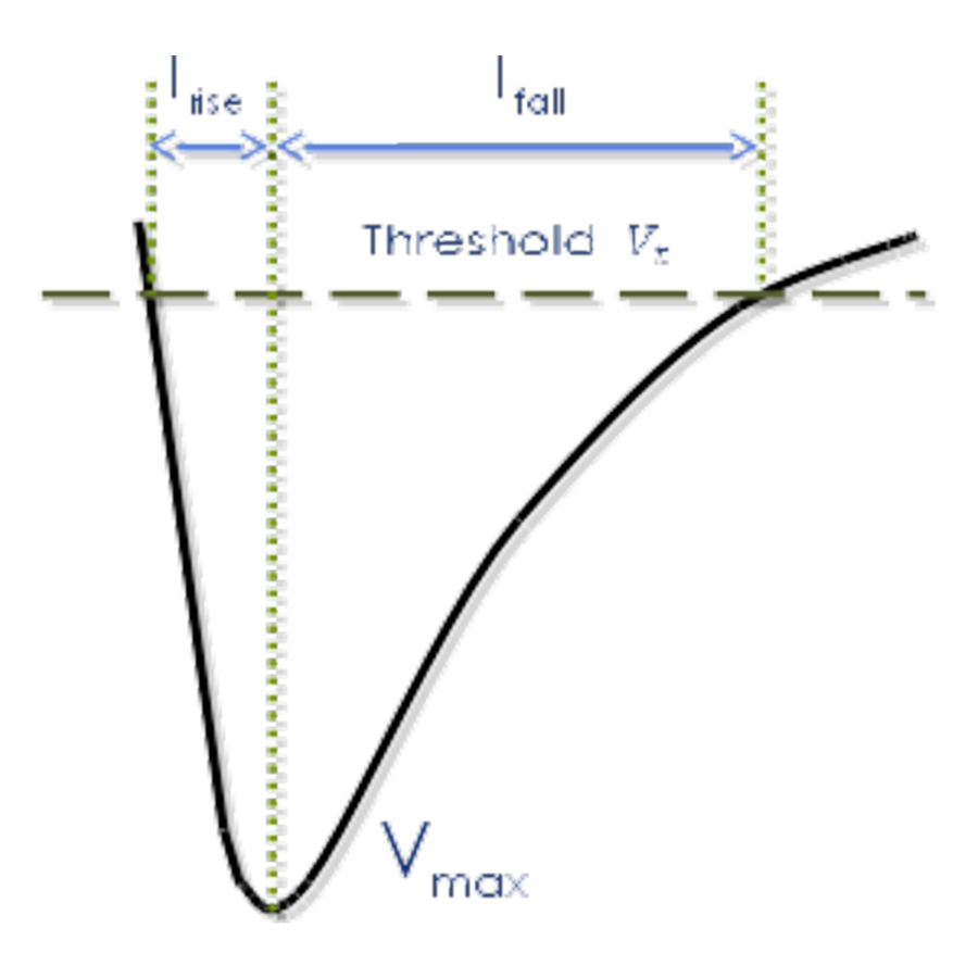
Figure 1: Time over threshold

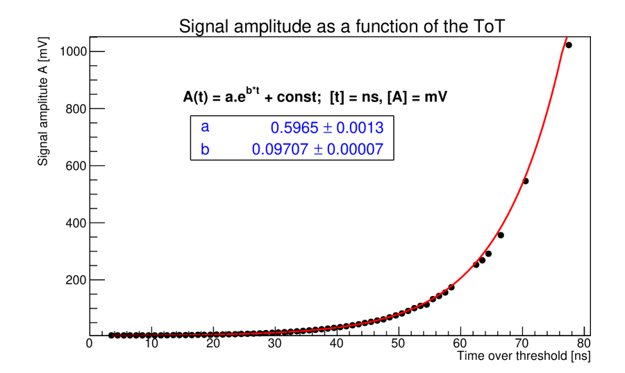
Figure 2: Relation between the time over threshold and signal amplitude. The relation between the signal amplitude and the deposited energy is linear.

While the charge or amplitude measurements is a well established and mature technique the ToT measurement is just becoming attractive nowadays due to the development of high precision time measurement devices - tens of picoseconds.

In the present article we describe the observation of a peculiar structure in the reconstructed distribution of the ToT which we could only explain by the superposition of a small amplitude sinusoidal noise on top of the PMT signal.

The charge measurement done by the QDC is completely immune to this effect as the integral of a sinusoidal function is zero.

2 Experimental setup

The present study was done at LNF-INFN as part of the development of the readout system of the Large Angle Photon vetoes for the NA62 experiment at CERN SPS [1].

The NA62 experiment aims to perform a 10% measurement of the branching fraction of the extremely rare decay $K^{+}\to\pi^{+}\bar{\nu}\nu$ and subsequently to measure the $V_{td}$ CKM matrix element. The theoretical prediction for that value is $Br(K^{+}\to\pi^{+}\bar{\nu}\nu)=(7.81\pm 0.80)*10^{-11}$. The very low rate requires an efficient veto of all the other charged kaon decay modes most of which contain photons in the final state. The usage of a 75 GeV kaon beam increases the minimal photon energy at which high rejection factor is necessary but still an inefficiency less that $10^{-4}$ is required for photons with energy of 100 MeV.

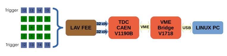
Figure 3: Schematics of the experimental setup for the measurement of the ToT distribution for cosmic rays with Lead-glass block.

The Large Angle Photon vetoes [2] consist of lead glass blocks made of Schott SF57 lead glass and are coupled to a R2238 photomultiplier. The blocks are arranged in the form of rings. A total of 12 Large Angle Photon vetoes were produced, with 5 or 4 rings for a total of about 2500 analog channels. The signal from a 100 MeV photon in the lead glass after propagation through the cables to the front end electronics could have an average amplitude as low as 10 mV and is almost equivalent to the response to the energy deposited by a minimally ionizing particle passing (MIP) through the crystal.

The front end electronics of the lead glass blocks was developed at the LNF [3]. It is based on a 9U VME mother board receiving 32 analog inputs. Each signal is clamped, amplified and split into two before being transferred to a high speed comparator with an LVDS output driver. The comparator threshold could be set through a board controller mezzanine, which provides a serial USB and a CAN-Open communication. The minimal effective threshold for all the channels was found to be less than 5 mV. An additional negative feedback circuit was implemented to dynamically decrease the absolute value of the threshold just after the leading edge of the signal. Such a mechanism, referred to as hysteresis, provides a safety margin against fast changing signals which would cause the digital LVDS output to oscillate.

The experimental setup used during these studies is shown in Fig. 3. The signals coming from the lead-glass blocks, after the discrimination, were readout by a V1190B TDC module which is based on the CERN HPTDC chip [5] and incorporates 2 times 32 input channels. The data is transferred to a PC for further analysis through a V1718 VME controller via a USB connection.

The recorded data showed a peculiar shape of the ToT distribution. An explanation based on the addition of a sinusoidal noise was employed and verified by means of a numerical signal simulation.

3 Signal and noise modeling

The general function describing the output signal would be

$$A(t)=\int_{0}^{t}I(t-\theta)*f(\theta)\leavevmode\nobreak\ d\theta,$$ (2)

where $I(t)$ is the intensity of the light produced in the active material and $f(t)$ is the photodetector response function to single electron. The form of the light intensity was chosen as an exponential decay with decay time $\tau$,

$$I(t)=\frac{N_{0}}{\tau}e^{-t/\tau},$$ (3)

assuming that the energy inside the active media is released instantly (true for small sized detectors) and the only contribution comes from light propagation or scintillating centers decay. The normalization $N_{0}$ is the number of the total photons emitted.

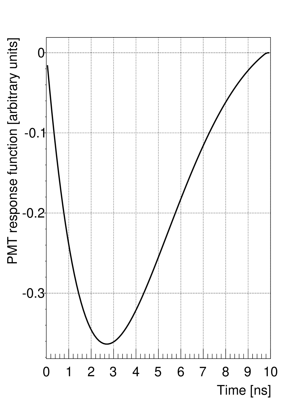
Figure 4: Single electron response function of the PMT

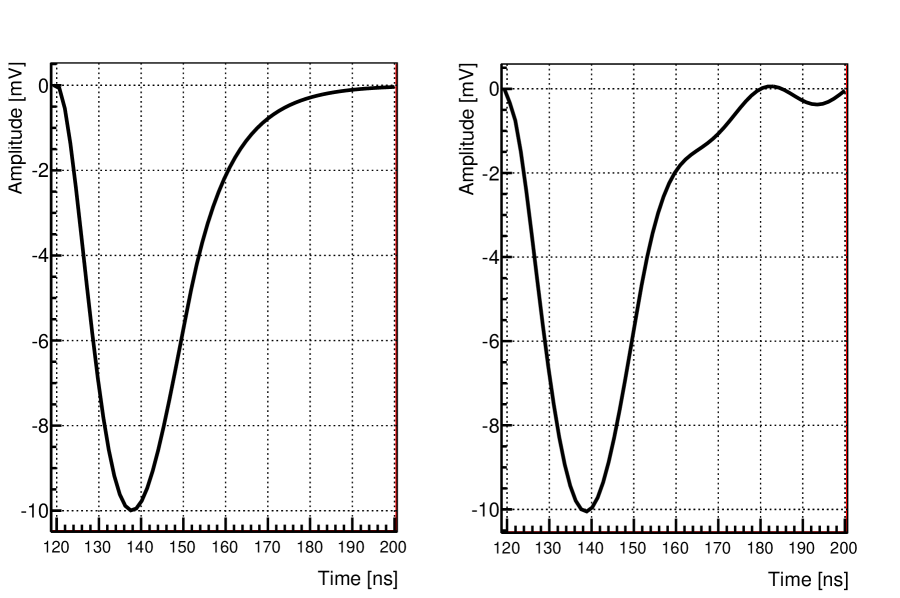
Figure 5: Shape of the output signal of the system Lead-Glass block - PMT without and with the addition of 300 $\mu$V noise.

The PMT single electron response was approximated with the function

$$f(\theta)=sin(a\theta)\times e^{-\theta/b},$$ (4)

where $a$ and $b$ were taken as free parameters. The use of such a function could be justified with an initial increase of the signal amplitude due to arrival of first electrons and further a decrease of the amplitude due to full charge collection at the anode of the PMT.

An advantage of using functions 3 and 4 is the simple and analytic form of the final signal. The resulting output signal amplitude at the anode of the PMT would then be described as

$$A(t)=\frac{-N_{0}}{a^{2}+c^{2}}\times\frac{e^{-t/\tau}}{\tau}\times\left[e^{ct}(c\leavevmode\nobreak\ sin(at)-a\leavevmode\nobreak\ cos(at))+a\right],$$ (5)

where $c=1/\tau-1/b$. The width of the signal $\Delta T$ is described by the parameters $a$ - $\Delta T=\pi/a$.

This signal model had been previously applied to describe the Eljen 212 scintillator coupled to Hamamatsu R6427 photomultiplier. The scintillator decay time constant, the PMT rise time and fall time were found to be consistent with the specification. Their behavior with the different PMT voltages were as expected. This check lead to the confidence of applying the chosen signal description to model the time over threshold behavior in various conditions.

The noise was simulated by adding a parasitic signal

$$A_{tot}(t)=A(t)\leavevmode\nobreak\ +\leavevmode\nobreak\ A_{noise}(t)=A(t)\leavevmode\nobreak\ +\leavevmode\nobreak\ A_{0}\leavevmode\nobreak\ sin(2\pi ft+\phi),$$ (6)

where $A_{0}$ is the noise amplitude, $f$ is the noise frequency and $\phi$ is a random chosen phase. The noise could either be picked-up from external sources or generated internally in the front end electronics by parasitic positive feedback. For the present studies the real origin of the noise is not important.

Thus the basic parameters used to describe the characteristics of the output signal were:

• Average signal amplitude. The signal amplitude was simulated as a Landau distribution with most probable value of 10 mV and a gaussian sigma of $\approx$2 mV. This corresponds to a total of 25 photoelectrons per MIP from the Lead-glass - PMT system.

• Threshold. The threshold was kept fixed during the simulation in order to see what was the additional effect of the hysteresis and the noise on top of the PMT signal. Two values were studied as examples - 5 mV and 7 mV.

• Hysteresis. The hysteresis is an important ingredient of the time over threshold circuit and it prevents short and oscillating output when the input signal is very close to the threshold. The hysteresis was varied from 0 mV to 3 mV in steps of 300 $\mu$V.

• Noise amplitude. The noise amplitude was varied from 0 mV to 3 mV in steps of 300 $\mu$V.

• Noise frequency. The noise frequency was kept fixed to 300 MHz as was independently observed with a digital oscilloscope.

The output quantity is the time over a certain threshold. A signal is considered to be detected if the time over threshold is longer than a fixed minimal time $\Theta_{0}$. In the present studies $\Theta_{0}=5$ ns was used, since it was compatible with the dead time of the HPTDC.

4 Results and discussions

With the described experimental setup the obtained time over threshold distribution is shown in Fig. 7. It possesses a bizarre feature of multiple peaks - a comb-like structure - which was initially puzzling and stimulated the presented study. Few explanations were considered ranging from effects due to energy deposit and photoelectron emission to TDC miss-functioning effects (stuck bit for example). Finally the data was reproduced exploiting the signal modeling described in section 3 with 300 MHz sinusoidal external (pick-up) noise on the input analog signals.

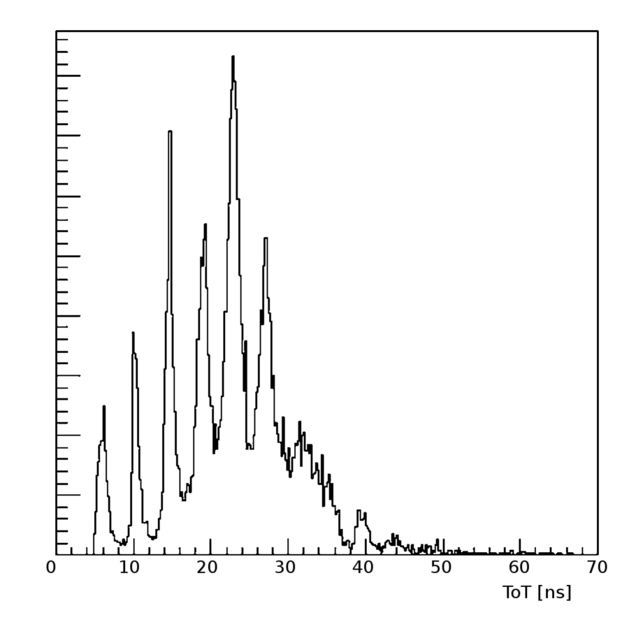
Figure 6: Measured time over a 10 mV threshold distribution for cosmic rays from a Lead-Glass block.

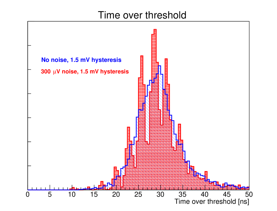
Figure 7: Simulated time over 5 mV threshold distribution for cosmic rays with external noise with amplitude of 300 $\mu$V

The effect on the inclusion of the extra noise is shown in Fig. 7. The blue line is the expected time over threshold distribution for a signal from the Lead-Glass block without noise and the red histogram is the result with the 300 $\mu$V noise. The sinusoidal noise induces a random shift on the measured leading edge or trailing edge alone but correlates them between each other - if the leading edge is crossed predominantly when the phase of the noise is $\pi/2$ the trailing edge is crossed when the phase is close to $3\pi/2$.

In a general setup the inclusion of noise doesn’t change the detection efficiency for a signal. In the case where there is a minimal detectable (5 ns in the case of HPTDC) the noise can induce inefficiency through artificially decreasing the ToT of the signals that are close to the threshold. If the period of the noise is smaller than the dead time of the TDC the situation becomes critical as in the case of HPTDC with 300 MHz noise. The inefficiency is partially recovered by the presence of hysteresis shifting forward the trailing edge but the effect could be dramatic as shown in Fig. 8.

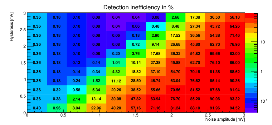
Figure 8: Dependence of the inefficiency on the value of the hysteresis as function of the amplitude of the input noise. An efficient hit is defined if the first leading and trailing edge form time over threshold longer than 5 ns.

The present studies underline the importance of the hysteresis to diminish the dependence on the external noise. The minimal hysteresis one should consider when employing ToT based solutions for readout electronics is 50% higher than the expected sinusoidal noise.

The noise induces an additional uncertainty to the measurement of the time over threshold which combines with the uncertainty from the underlying physics process - the shower development and primary charge generation. While the uncertainty of the latter usually scales as the square root of the deposited energy (due to linear scale of the primary charges), the uncertainty due to the noise is constant in the time over threshold variable - $\Delta\Theta=const$. $\Delta\Theta$ can be assumed to be half of the distance between two consecutive clusterisation peaks, as seen in Fig. 7. Then the physics quantity, the energy ($E\sim A$), will acquire an additional constant term in the resolution dependence as a function of energy

$$\frac{\Delta E}{E}(E)_{ToT}=\frac{\Delta A}{A}(E)_{ToT}=b*\Delta\Theta=const.$$ (7)

This term could be as high as tens of percent ($b\sim 0.1$ ns^-1 and $\Delta\Theta\sim 1.5$ ns in this study) and will be the dominant one, especially in the measurement of the electromagnetic showers where the stochastic and the noise terms are usually quite low.

5 Conclusions

A comb-like structure was identified in the time over threshold distribution in cosmic ray data for a first time, was explained to be caused by the pick up of high frequency low amplitude noise, and was modeled successfully. The effect should be taken into account by every detector readout system aiming to use ToT as a measurable quantity to describe the data from the detector. In the case of the Large Angle Vetoes readout system additional precautions were taken (better cable shielding, extra noise filtering in the crate power supply) to decrease the level of the noise to an acceptable level, which does not degrade the efficiency of the system.

References

- [1] F. Hahn et al. [NA62 Collaboration], http://cds.cern.ch/record/1404985.
- [2] P. Massarotti et al., PoS ICHEP 2012, 504 (2013).
- [3] A. Antonelli et al., JINST 8 (2013) C01020.
- [4] F. Gonnella et al., PoS TIPP 2014 397 (2014).
-
[5]
J. Christiansen, High Performance Time to Digital Converter,
http://tdc.web.cern.ch/TDC/hptdc/docs/hptdc_manual_ver2.2.pdf