How Many Communities Are There?

Abstract

Stochastic blockmodels and variants thereof are among the most widely used approaches to community detection for social networks and relational data. A stochastic blockmodel partitions the nodes of a network into disjoint sets, called communities. The approach is inherently related to clustering with mixture models; and raises a similar model selection problem for the number of communities. The Bayesian information criterion (BIC) is a popular solution, however, for stochastic blockmodels, the conditional independence assumption given the communities of the endpoints among different edges is usually violated in practice. In this regard, we propose composite likelihood BIC (CL-BIC) to select the number of communities, and we show it is robust against possible misspecifications in the underlying stochastic blockmodel assumptions. We derive the requisite methodology and illustrate the approach using both simulated and real data. Supplementary materials containing the relevant computer code are available online.

Key Words: Community detection; Composite likelihood; Degree-corrected stochastic blockmodel; Model selection; Spectral clustering; Stochastic blockmodel.

.   ntroduction

Enormous network datasets are being generated and analyzed along with an increasing interest from researchers in studying the underlying structures of a complex networked world. The potential benefits span traditional scientific fields such as epidemiology and physics, but also emerging industries, especially large-scale internet companies. Among a variety of interesting problems arising with network data, in this paper, we focus on community detection in undirected networks $G:=(V,E)$, where $V$ and $E$ are the sets of nodes and edges, respectively. In this framework, the community detection problem can be formulated as finding the true disjoint partition of $V=V_{1}\sqcup\cdots\sqcup V_{K}$, where $K$ is the number of communities. Although it is difficult to give a rigorous definition, communities are often regarded as tightly-knit groups of nodes which are loosely connected between themselves.

The community detection problem has close connections with graph partitioning, which could be traced back to Euler, while it has its own characteristics due to the concrete physical meanings from the underlying dataset (Newman and Girvan, 2004). Over the last decade, there has been a considerable amount of work on it, including minimizing ratio cut (Wei and Cheng, 1989), minimizing normalized cut (Shi and Malik, 2000), maximizing modularity (Newman and Girvan, 2004), hierarchical clustering (Newman, 2004) and edge-removal methods (Newman and Girvan, 2004), to name a few. Among all the progress made by peer researchers, spectral clustering (Donath and Hoffman, 1973) based on stochastic blockmodels (Holland et al., 1983) debuted and soon gained a majority of attention. We refer the interested readers to Spielmat and Teng (1996) and Goldenberg et al. (2010) as comprehensive reviews on the history of spectral clustering and stochastic blockmodels, respectively.

Compared to the amount of work on spectral clustering or stochastic blockmodels, to the best of our knowledge, there is little work on the selection of the community number $K$. In most of the previously mentioned community detection methods, the number of communities is generally input as a pre-specified quantity. For the literature addressing the problem of selecting $K$, besides the block-wise edge splitting method of Chen and Lei (2014), a common practice is to use BIC-type criteria (Airoldi et al., 2008; Daudin et al., 2008) or a variational Bayes approach (Latouche et al., 2012; Hunter et al., 2012). An inherently related problem is that of selecting the number of components in mixture models, where the birth-and-death point process of Stephens (2000) and the allocation sampler of Nobile and Fearnside (2007) provide two fully Bayesian approaches in the case where $K$ is finite but unknown. Based on the allocation sampler, McDaid et al. (2013) propose an efficient Bayesian clustering algorithm which directly estimates the number of communities in stochastic blockmodels, and which exhibits similar results to the variational Bayes approach of Latouche et al. (2012). Nonparametric Bayesian methods based on Dirichlet process mixtures (Ferguson, 1973) have also been used to estimate the number of components in this finite but unknown $K$ setting (Fearnhead, 2004), although the inconsistency of this approach has been recently shown by Miller and Harrison (2014). This community or mixture component number $K$, as a vital part of model selection procedures, highly depends on the model assumptions. For instance, the famous stochastic blockmodel has undesirable restrictive assumptions in the form of independent Bernoulli observations when the community assignments are known.

In this paper, we study the community number selection problem with robustness consideration against model misspecification in the stochastic blockmodel and its variants. Our motivation is that, the conditional independence assumption among edges, when the communities of their endpoints are given, is usually violated in real applications. In addition, we do not restrict our interest only to exchangeable graphs. Using techniques from the composite likelihood paradigm (Lindsay, 1988), we develop a composite likelihood BIC (CL-BIC) approach (Gao and Song, 2010) for selecting the community number in the situation where assumed independencies in the stochastic blockmodel and other exchangeable graph models do not hold. The procedure is tested on simulated and real data, and is shown to outperform two competitors – traditional BIC and the variational Bayes criterion of Latouche et al. (2012), in terms of model selection consistency.

The rest of the paper is organized as follows. The background for stochastic blockmodels and spectral clustering is introduced in Section 2, and the proposed CL-BIC methodology is developed in Section 3. In Section 4, several simulation examples as well as two real data sets are analyzed. The paper is concluded with a short discussion in Section 5.

.   ackground

First, we would like to introduce some notation. For an $N$-node undirected, simple, and connected network $G$, its symmetric adjacency matrix $\boldsymbol{A}$ is defined as $A_{ij}:=1$ if $(i,j)$ is an element in $E$, and $A_{ij}:=0$ otherwise. The diagonal $\{A_{ii}\}_{i=1}^{N}$ is fixed to zero (i.e., self-edges are not allowed). Moreover, $\boldsymbol{D}$ and $\boldsymbol{L}$ denote the degree matrix and Laplacian matrix, respectively. Here, ${D}_{ii}:=d_{i}$, and ${D}_{ij}:=0$ for $i\neq j$, where $d_{i}$ is the degree of node $i$, i.e., the number of edges with endpoint node $i$; and $\boldsymbol{L}:=\boldsymbol{D}^{-1/2}\boldsymbol{A}\boldsymbol{D}^{-1/2}$. As isolated nodes are discarded, $\boldsymbol{D}^{-1/2}$ is well-defined.

2.1 Stochastic Blockmodels

2.1.1 Standard Stochastic Blockmodel

Stochastic blockmodels were first introduced in Holland et al. (1983). They posit independent Bernoulli random variables $\{A_{ij}\}_{1\leq i<j\leq N}$ with success probabilities $\{P_{ij}\}$ which depend on the communities of their endpoints $i$ and $j$. Consequently, all edges are conditionally independent given the corresponding communities. Moreover, each node is associated with one and only one community, with label $Z_{i}$, where $Z_{i}\in\{1,\ldots,K\}$. Following Rohe et al. (2011) and Choi et al. (2012), throughout this paper we assume each $Z_{i}$ is fixed and unknown, thus yielding $\mathbb{P}(A_{ij}=1;Z_{i}=z_{i},Z_{j}=z_{j})=\theta_{z_{i}z_{j}}$. Treating the node assignments $Z_{1},\ldots,Z_{N}$ as latent random variables is another popular approach in the community detection literature, and various methods including the variational Bayes criterion of Latouche et al. (2012) and the belief propagation algorithm of Decelle et al. (2011) efficiently approximate the corresponding observed-data log-likelihood of the stochastic blockmodel, without having to add $K^{N}$ multinomial terms accounting for all possible label assignments.

For $\boldsymbol{\theta}:=(\theta_{ab};1\leq a\leq b\leq K)^{\prime}$ and for any fixed community assignment $\boldsymbol{z}\in\{1,\ldots,K\}^{N}$, the log-likelihood under the standard Stochastic Blockmodel (SBM) is given as

$$\ell(\boldsymbol{\theta};\boldsymbol{A}):=\sum_{i<j}[A_{ij}\log\theta_{z_{i}z_{j}}+(1-A_{ij})\log(1-\theta_{z_{i}z_{j}})].$$ (1)

For the remainder of the paper, denote $N_{a}$ as the size of community $a$, and $n_{ab}$ as the maximum number of possible edges between communities $a$ and $b$, i.e., $n_{ab}:=N_{a}N_{b}$ for $a\neq b$, and $n_{aa}:=N_{a}(N_{a}-1)/2$. Also, let $m_{ab}:=\sum_{i<j}A_{ij}\boldsymbol{1}\{z_{i}=a,z_{j}=b\}$, and $\hat{\theta}_{ab}:=m_{ab}/n_{ab}$ be the MLE of $\theta_{ab}$ in (1).

Under this framework, Choi et al. (2012) showed that the fraction of misclustered nodes converges in probability to zero under maximum likelihood fitting when $K$ is allowed to grow no faster than $\sqrt{N}$. By means of a regularized maximum likelihood estimation approach, Rohe et al. (2014) further proved that this weak convergence can be achieved for $K=\mathcal{O}(N/\log^{5}N)$.

2.1.2 Degree-Corrected Stochastic Blockmodel

Heteroscedasticity of node degrees within communities is often observed in real-world networks. To tackle this problem, Karrer and Newman (2011) proposed the Degree-Corrected Blockmodel (DCBM), in which the success probabilities $\{P_{ij}\}$ are also functions of individual effects. To be more precise, the DCBM assumes that $\mathbb{P}(A_{ij}=1;Z_{i}=z_{i},Z_{j}=z_{j})=\omega_{i}\omega_{j}\theta_{z_{i}z_{j}}$, where $\boldsymbol{\omega}:=(\omega_{1},\ldots,\omega_{n})^{\prime}$ are individual effect parameters satisfying the identifiability constraint $\sum_{i}\omega_{i}\boldsymbol{1}\{z_{i}=a\}=1$ for each community $1\leq a\leq K$.

To simplify technical derivations, Karrer and Newman (2011) allowed networks to contain both multi-edges and self-edges. Thus, they assumed the random variables $\{A_{ij}\}_{1\leq i\leq j\leq N}$ to be independent Poisson, with the previously defined success probabilities $\{P_{ij}\}$ of an edge between vertices $i$ and $j$ replaced by the expected number of such edges. Under this framework, and for any fixed community assignment $\boldsymbol{z}\in\{1,\ldots,K\}^{N}$, Karrer and Newman (2011) arrived at the log-likelihood $\ell(\boldsymbol{\theta,\omega};\boldsymbol{A})$ of observing the adjacency matrix $\boldsymbol{A}=(A_{ij})$ under the DCBM,

$$\ell(\boldsymbol{\theta,\omega};\boldsymbol{A}):=2\sum_{i}d_{i}\log\omega_{i}+\sum_{a,b}(m_{ab}\log\theta_{ab}-\theta_{ab}).$$ (2)

After allowing for the identifiability constraint on $\boldsymbol{\omega}$, the MLEs of the parameters $\theta_{ab}$ and $\omega_{i}$ are given by $\hat{\theta}_{ab}:=m_{ab}$ and $\hat{\omega}_{i}:=d_{i}/\sum_{j:z_{j}=z_{i}}d_{j}$, respectively.

As mentioned in Zhao et al. (2012), there is no practical difference in performance between the log-likelihood (2) and its slightly more elaborate version based on the true Bernoulli observations. The reason is that the Bernoulli distribution with a small mean is well approximated by the Poisson distribution, and the sparser the network is, the better the approximation works (Perry and Wolfe, 2012).

2.1.3 Mixed Membership Stochastic Blockmodel

As a methodological extension in which nodes are allowed to belong to more than one community, Airoldi et al. (2008) proposed the Mixed Membership Stochastic Blockmodel (MMB) for directed relational data $\{A_{ij}\}_{1\leq i,j\leq N}$. For instance, when a social actor interacts with its different neighbors, an array of different social contexts may be taking place and thus the actor may be taking on different latent roles.

The model assumes the observed network is generated according to node-specific distributions of community membership and edge-specific indicator vectors denoting membership in one of the $K$ communities. More specifically, each vertex $i$ is associated with a randomly drawn vector $\vec{\boldsymbol{\pi}}_{i}$, with $\pi_{ia}$ denoting the probability of node $i$ belonging to community $a$. Additionally, let the indicator vector $\vec{\boldsymbol{z}}_{i\rightarrow j}$ denote the community membership of node $i$ when he sends a message to node $j$, and $\vec{\boldsymbol{z}}_{i\leftarrow j}$ denote the community membership of node $j$ when he receives a message from node $i$. If, in order to account for the asymmetric interactions, we denote by $\boldsymbol{\theta}:=(\theta_{ab})$ the $K\times K$ matrix where $\theta_{ab}$ represents the probability of having an edge from a social actor in community $a$ to a social actor in community $b$, the MMB posits that the $\{A_{ij}\}_{1\leq i,j\leq N}$ are drawn from the following generative process.

• For each node $i\in V$:

  • Draw a $K$ dimensional mixed membership vector $\vec{\boldsymbol{\pi}}_{i}\sim\text{Dirichlet}(\boldsymbol{\alpha})$, with the vector $\boldsymbol{\alpha}=(\alpha_{1},\ldots,\alpha_{K})^{\prime}$ being a hyper-parameter.

• For each possible edge variable ${A_{ij}}$:

  • Draw membership indicator vector for the initiator $\vec{\boldsymbol{z}}_{i\rightarrow j}\sim\text{Multinomial}(\vec{\boldsymbol{\pi}}_{i})$.

  • Draw membership indicator vector for the receiver $\vec{\boldsymbol{z}}_{i\leftarrow j}\sim\text{Multinomial}(\vec{\boldsymbol{\pi}}_{j})$.

  • Sample the interaction $A_{ij}\sim\text{Bernoulli}(\vec{\boldsymbol{z}}_{i\rightarrow j}^{\prime}\boldsymbol{\theta}\vec{\boldsymbol{z}}_{i\leftarrow j})$.

Upon defining the set of mixed membership vectors $\boldsymbol{\Pi}:=\{\vec{\boldsymbol{\pi}}_{i}:i\in V\}$ and the sets of membership indicator vectors $\boldsymbol{Z}_{\rightarrow}:=\{\vec{\boldsymbol{z}}_{i\rightarrow j}:i,j\in V\}$ and $\boldsymbol{Z}_{\leftarrow}:=\{\vec{\boldsymbol{z}}_{i\leftarrow j}:i,j\in V\}$, following Airoldi et al. (2008), we obtain the complete data log-likelihood of the hyper-parameters $\{\boldsymbol{\theta},\boldsymbol{\alpha}\}$ as

$$\ell(\boldsymbol{\theta,\alpha};\boldsymbol{A},\boldsymbol{\Pi},\boldsymbol{Z}_{\rightarrow},\boldsymbol{Z}_{\leftarrow}) :=\sum_{i,j}[A_{ij}\log(\vec{\boldsymbol{z}}_{i\rightarrow j}^{\prime}\boldsymbol{\theta}\vec{\boldsymbol{z}}_{i\leftarrow j})+(1-A_{ij})\log(1-\vec{\boldsymbol{z}}_{i\rightarrow j}^{\prime}\boldsymbol{\theta}\vec{\boldsymbol{z}}_{i\leftarrow j})]$$ (3)

$$\mkern-10.0mu+N\Big{(}\log\Gamma(\sum_{a}\alpha_{a})-\sum_{a}\log\Gamma(\alpha_{a})\Big{)}+\sum_{i}\sum_{a}(\alpha_{a}-1)\log\pi_{ia}+\text{const},$$

where $\boldsymbol{A}$ corresponds to the observed data and $\{\boldsymbol{\Pi},\boldsymbol{Z}_{\rightarrow},\boldsymbol{Z}_{\leftarrow}\}$ are the latent variables.

In order to carry out posterior inference of the latent variables given the observations $\boldsymbol{A}$, Airoldi et al. (2008) proposed an efficient coordinate ascent algorithm based on a variational approximation to the true posterior. Therefore, one can compute expected posterior mixed membership vectors and posterior membership indicator vectors. We refer interested readers to Section 3 in Airoldi et al. (2008) for further details.

Consequently, following the same profile likelihood approach, for any fixed set $\{\boldsymbol{\Pi},\boldsymbol{Z}_{\rightarrow},\boldsymbol{Z}_{\leftarrow}\}$, the MLE of $\theta_{ab}$ is given by

$$\hat{\theta}_{ab}:=\sum_{i,j}A_{ij}\cdot\vec{\boldsymbol{z}}_{i\rightarrow j,a}\vec{\boldsymbol{z}}_{i\leftarrow j,b}\bigg{/}\sum_{i,j}\vec{\boldsymbol{z}}_{i\rightarrow j,a}\vec{\boldsymbol{z}}_{i\leftarrow j,b}.$$ (4)

As the MLE of $\alpha_{a}$ does not admit a closed form, Minka (2000) proposed an efficient Newton-Raphson procedure for obtaining parameter estimates in Dirichlet models, where the gradient and Hessian matrix of the complete data log-likelihood (3) with respect to $\boldsymbol{\alpha}$ are

$$\frac{\partial\ell(\boldsymbol{\theta,\alpha};\boldsymbol{A})}{\partial\alpha_{a}}= \,\,N\Big{(}\Psi(\sum_{a}\alpha_{a})-\Psi(\alpha_{a})\Big{)}+\sum_{i}\sum_{a}\log\pi_{ia}$$ (5)

$$\frac{\partial^{2}\ell(\boldsymbol{\theta,\alpha};\boldsymbol{A})}{\partial\alpha_{a}\partial\alpha_{b}}= \,\,N\Big{(}\Psi^{\prime}(\sum_{a}\alpha_{a})-\Psi^{\prime}(\alpha_{a})\boldsymbol{1}\{a=b\}\Big{)},$$

and $\Psi$ is known as the digamma function (i.e., the logarithmic derivative of the gamma function).

2.2 Spectral Clustering and SCORE

Although there is a parametric framework for the standard stochastic blockmodel, considering the computational burden, it is intractable to directly estimate both parameters $\boldsymbol{\theta}$ and $\boldsymbol{z}$ based on exact maximization of the log-likelihood (1). Researchers have instead resorted to spectral clustering as a computationally feasible algorithm. For comprehensive reviews, we refer interested readers to von Luxburg (2007) and Rohe et al. (2011), in which the authors proved the consistency of spectral clustering in the standard stochastic blockmodel under proper conditions imposed on the density of the network and the eigen-structure of the Laplacian matrix. The algorithm finds the eigenvectors $\boldsymbol{u_{1}},\ldots,\boldsymbol{u_{K}}$ associated with the $K$ eigenvalues of $\boldsymbol{L}$ that are largest in magnitude, forming an $N\times K$ matrix $\boldsymbol{U}:=(\boldsymbol{u_{1}},\ldots,\boldsymbol{u_{K}})$, and then applies the $K$-means algorithm to the rows of $\boldsymbol{U}$.

Similarly, Jin (2015) proposed a variant of spectral clustering for the DCBM, called Spectral Clustering On Ratios-of-Eigenvectors (SCORE). Instead of using the Laplacian matrix $\boldsymbol{L}$, SCORE collects the eigenvectors $\boldsymbol{v_{1}},\ldots,\boldsymbol{v_{K}}$ associated with the $K$ eigenvalues of $\boldsymbol{A}$ that are largest in magnitude, and then forms the $N\times K$ matrix $\boldsymbol{V}:=(\boldsymbol{1},\boldsymbol{v_{2}}/\boldsymbol{v_{1}},\ldots,\boldsymbol{v_{K}}/\boldsymbol{v_{1}})$, where the division operator is taken entry-wise, i.e., for vectors $\boldsymbol{a},\boldsymbol{b}\in\mathbb{R}^{n}$, with $\Pi_{\ell=1}^{n}b_{\ell}\neq 0$, $\boldsymbol{a}/\boldsymbol{b}:=(a_{1}/b_{1},\ldots,a_{n}/b_{n})^{\prime}$. SCORE then applies the $K$-means algorithm to the rows of $\boldsymbol{V}$. The corresponding consistency results for the DCBM are also provided in Jin (2015).

.   odel Selection for the Number of Communities

3.1 Motivation

In much of the previous work, e.g. Airoldi et al. (2008), Daudin et al. (2008) and Handcock et al. (2007), researchers have used a BIC-penalized version of the log-likelihood (1) to choose the community number $K$. However, we are aware of the possible misspecifications in the underlying stochastic blockmodel assumptions and in the loss of precision from the computational relaxation brought in by spectral clustering.

Firstly, in network data, edges are not necessarily independent if only the communities of their endpoints are given. For instance, if two different edges $A_{ij}$ and $A_{il}$ have mutual endpoint $i$, it is highly likely that they are dependent even given the community labels of their endpoints. This misspecification problem exists in both the standard stochastic blockmodel and its variants, such as DCBM (Karrer and Newman, 2011) and MMB (Airoldi et al., 2008). Secondly, as previously mentioned, spectral clustering is a feasible relaxation, but the loss of precision is inevitable. Several examples of this can be found in Guattery and Miller (1998). Whence, we resort to introducing CL-BIC with the concern of robustness against misspecifications in the underlying stochastic blockmodel.

We would like to emphasize that CL-BIC is not a new community detection method. Instead, under the SBM, DCBM, or MMB assumptions, it can be combined with existing community detection methods to choose the true community number.

3.2 Composite Likelihood Inference

The CL-BIC approach extends the concepts and theory of conventional BIC on likelihoods to the composite likelihood paradigm (Lindsay, 1988; Varin et al., 2011). Composite likelihood aims at a relaxation of the computational complexity of statistical inference based on exact likelihoods. For instance, when the dependence structure for relational data is too complicated to implement, a working independence assumption can effectively recover some properties of the usual maximum likelihood estimators (Cox and Reid, 2004; Varin et al., 2011). However, under this misspecification framework, the asymptotic variance of the resulting estimators is usually underestimated as the Fisher information. Composite marginal likelihoods (also known as independence likelihoods) have the same formula as conventional likelihoods in terms of being a product of marginal densities (Varin, 2008), while statistical inference based on them can capture this loss of variance. Consequently, to pursue the “true” model, CL-BIC penalizes the number of parameters more than what BIC does for dependent relational data.

Before going into details, we would like to give the rationale of using stochastic blockmodels under a misspecification framework. In order to estimate the true joint density $g$ of $\{A_{ij}\}_{1\leq i<j\leq N}$, we consider the stochastic blockmodel family $\mathscr{P}=\{p_{\boldsymbol{\theta}}:\boldsymbol{\theta}\in\Theta\}$, where $\Theta=[0,1]^{K(K+1)/2}$ for the standard stochastic blockmodel, and $\Theta=[0,1]^{K(K+1)/2+N}$ for DCBM. The true joint density $g$ may or may not belong to $\mathscr{P}$, which is a parametric family imposing independence among the $\{A_{ij}\}_{i<j}$ when only the communities of the endpoints are given.

Due to the difficulty in specifying the full, highly structured ${N\choose 2}$-dimensional density $g$, while having access to the univariate densities $p_{ij}(\cdot;\boldsymbol{\theta})$ of $A_{ij}$ under the blockmodel family $\mathscr{P}$, the composite marginal likelihood paradigm compounds the first-order log-likelihood contributions to form the composite log-likelihood

$$\text{cl}(\boldsymbol{\theta};\boldsymbol{A}):=\sum_{i<j}\log\,p_{ij}(A_{ij};\boldsymbol{\theta}),$$ (6)

where $\text{cl}(\cdot;\boldsymbol{A})$ corresponds to (1) under the standard stochastic blockmodel, and corresponds to (2) in the DCBM framework. Since each component of $\text{cl}(\boldsymbol{\theta};\boldsymbol{A})$ in (6) is a valid log-likelihood object, the composite score estimating equation $\nabla_{\boldsymbol{\theta}}\,\text{cl}(\boldsymbol{\theta};\boldsymbol{A})=0$ is unbiased under usual regularity conditions. The associated Composite Likelihood Estimator (CLE) $\boldsymbol{\hat{\theta}}_{\text{C}}$, defined as the solution to $\nabla_{\boldsymbol{\theta}}\,\text{cl}(\boldsymbol{\theta};\boldsymbol{A})=0$, suggests a natural estimator of the form $\hat{p}=p_{\boldsymbol{\hat{\theta}}_{\text{C}}}$ to minimize the expected composite Kullback–Leibler divergence (Varin and Vidoni, 2005) between the assumed blockmodel $p_{\boldsymbol{\theta}}$ and the true, but unknown, joint density $g$,

$$\Delta_{\text{C}}(g,p;\boldsymbol{\theta}):=\sum_{i<j}\mathbb{E}_{g}(\log\,g(\{A_{ij}\}_{i<j}\in\mathscr{A}_{ij})-\log\,p_{ij}(A_{ij};\boldsymbol{\theta})),$$

where $\{\mathscr{A}_{ij}\}_{i<j}$ denotes the corresponding set of marginal events.

In terms of the asymptotic properties of the CLE, following the discussion in Cox and Reid (2004), it is important to distinguish whether the available data consist of many independent replicates from a common distribution function or form a few individually large sequences. While, in the first scenario, consistency and asymptotic normality of the corresponding $\boldsymbol{\hat{\theta}}_{\text{C}}$ hold under some regularity conditions from the classical theory of estimating equations (Varin et al., 2011), some difficulties arise in the second one, which includes our observations $\{A_{ij}\}_{i<j}$. Indeed, as argued in Cox and Reid (2004), if there is too much internal correlation present among the individual components of the composite score $\nabla_{\boldsymbol{\theta}}\,\text{cl}(\boldsymbol{\theta};\boldsymbol{A})$, the estimator $\boldsymbol{\hat{\theta}}_{\text{C}}$ will not be consistent. The CLE will retain good properties as long as the data are not too highly correlated, which is the case for spatial data with exponential correlation decay. Under this setting, Heagerty and Lele (1998) proved consistency and asymptotic normality of $\boldsymbol{\hat{\theta}}_{\text{C}}$ in a scenario where the data are not sampled independently from a study population. Under more general settings, consistency results are expected upon using limit theorems and parametric estimation for fields (e.g. Guyon, 1995); however, applying the corresponding results requires a properly defined distance on networks and $\alpha$-mixing conditions based on such distance.

3.3 Composite Likelihood BIC

Taking into account the measure of model complexity in the context of composite marginal likelihoods (Varin and Vidoni, 2005), we define the following criterion for selecting the community number $K$:

$$\text{CL-BIC}_{k}:=-2\,\text{cl}(\boldsymbol{\hat{\theta}}_{\text{C}};\boldsymbol{A})+d_{k}^{*}\log\left(N(N-1)/2\right),$$ (7)

where $k$ is the number of communities under consideration in the current model used as model index, $d^{*}_{k}:=\text{trace}(\boldsymbol{H}_{k}^{-1}\boldsymbol{V}_{k})$, $\boldsymbol{H}_{k}:=E_{\boldsymbol{\theta}}(-\nabla_{\boldsymbol{\theta}}^{2}\,\text{cl}(\boldsymbol{\theta};\boldsymbol{A}))$ and $\boldsymbol{V}_{k}:=\text{Var}_{\boldsymbol{\theta}}(\nabla_{\boldsymbol{\theta}}\,\text{cl}(\boldsymbol{\theta};\boldsymbol{A}))$. Then the resulting estimator for the community number is

$$\hat{k}_{CL-BIC}:=\operatorname*{arg\,min}_{k}\text{CL-BIC}_{k}.$$

Note that the CLE is a function of $k$, since a different model index yields a different estimator $\boldsymbol{\hat{\theta}}_{\text{C}}:=\boldsymbol{\hat{\theta}}_{\text{C}}(k)$. Assuming independent and identically distributed data replicates, which lead to consistent and asymptotically normally distributed estimators $\boldsymbol{\hat{\theta}}_{\text{C}}$, Gao and Song (2010) established the model selection consistency of a similar composite likelihood BIC approach for high-dimensional parametric models. While allowing for the number of potential model parameters to increase to infinity, their consistency result only holds when the true model sparsity is bounded by a universal constant.

Even though, under a misspecification framework for the blockmodel family $\mathscr{P}$, the observed data $\{A_{ij}\}_{i<j}$ do not form independent replicates from a common population, we anticipate the CL-BIC criterion (7) to be consistent in selecting the true community number $K$, at least when the correlation among the $\{A_{ij}\}_{i<j}$ is not severe and the estimators $\boldsymbol{\hat{\theta}}_{\text{C}}$ are consistent and asymptotically normal, as in Heagerty and Lele (1998). Since all the moment conditions in the consistency results from Gao and Song (2010) hold automatically after noticing the specific forms of the blockmodel composite log-likelihoods (1) – (3), under a properly defined mixing condition on $\{A_{ij}\}_{i<j}$ (Guyon, 1995), and for a bounded community number $K\leq k_{0}$, we conjecture that $\mathbb{P}\{\hat{k}_{CL-BIC}=K\}\rightarrow 1$ as the number of nodes $N$ in the network grows to infinity. This theoretical study will be relegated as a future work.

3.4 Formulae

3.4.1 Standard Stochastic Blockmodel

Following our discussions in the previous section, we treat (1) as the composite marginal likelihood, under the working independence assumption that, given the community labels of their endpoints, the Bernoulli random variables $\{A_{ij}\}_{i<j}$ are independent. The first-order partial derivative of $\ell(\boldsymbol{\theta};\boldsymbol{A})$ with respect to $\boldsymbol{\theta}$ is denoted as $\boldsymbol{u}(\boldsymbol{\theta})=(u(\theta_{ab});1\leq a\leq b\leq k)^{\prime}$, where

$$u(\theta_{ab})=\sum_{i<j}\left[\frac{A_{ij}}{\theta_{z_{i}z_{j}}}-\frac{1-A_{ij}}{1-\theta_{z_{i}z_{j}}}\right]\boldsymbol{I}^{a,b}_{i,j},$$

and

$$\boldsymbol{I}^{a,b}_{i,j}=\min\left(\mathbbm{1}\{z_{i}=a,z_{j}=b\}+\mathbbm{1}\{z_{i}=b,z_{j}=a\},1\right).$$

Furthermore, the second-order partial derivative of $\ell(\boldsymbol{\theta};\boldsymbol{A})$ has the following components,

$$\frac{\partial^{2}\ell(\boldsymbol{\theta};\boldsymbol{A})}{\partial\theta_{a_{1}b_{1}}\partial\theta_{a_{2}b_{2}}}=0,\;\text{ if }(a_{1},b_{1})\neq(a_{2},b_{2})$$

and

$$\hskip 37.5807pt\frac{\partial^{2}\ell(\boldsymbol{\theta};\boldsymbol{A})}{\partial\theta_{ab}^{2}}=-\sum_{i<j}\left[\frac{A_{ij}}{\theta^{2}_{z_{i}z_{j}}}+\frac{1-A_{ij}}{(1-\theta_{z_{i}z_{j}})^{2}}\right]\boldsymbol{I}^{a,b}_{i,j}.$$

Define the Hessian matrix $\boldsymbol{H}_{k}(\boldsymbol{\theta})=E_{\boldsymbol{\theta}}(-\partial\boldsymbol{u}(\boldsymbol{\theta})/\partial\boldsymbol{\theta})$, then

$$\boldsymbol{H}_{k}(\boldsymbol{\theta})=E_{\boldsymbol{\theta}}\left(\text{diag}\left\{-\partial^{2}\ell(\boldsymbol{\theta};\boldsymbol{A})/\partial\theta_{ab}^{2};1\leq a\leq b\leq k\right\}\right).$$

Define the variability matrix $\boldsymbol{V}_{k}(\boldsymbol{\theta})=\text{Var}_{\boldsymbol{\theta}}(\boldsymbol{u}(\boldsymbol{\theta}))$ and, following Varin and Vidoni (2005), the model complexity $d_{k}^{*}=\text{trace}[\boldsymbol{H}_{k}(\boldsymbol{\theta})^{-1}\boldsymbol{V}_{k}(\boldsymbol{\theta})]$. If the underlying model is indeed a correctly specified standard stochastic blockmodel, we have $d_{k}^{*}=k(k+1)/2$ and CL-BIC reduces to the traditional BIC. Indexed by $1\leq k\leq k_{0}$, the estimated criterion functions for the CL-BIC sequence (7) are

$$\widehat{\text{CL-BIC}_{k}}=-2\,\text{cl}(\boldsymbol{\hat{\theta}}_{\text{C}};\boldsymbol{A})+\hat{d}^{*}_{k}\log\left(N(N-1)/2\right),$$ (8)

where $\boldsymbol{\hat{\theta}}_{\text{C}}$ and $\hat{d}^{*}_{k}$ are estimators of $\boldsymbol{\theta}$ and $d^{*}_{k}$, respectively. For a certain $k$, the explicit estimator forms are given below:

$$\boldsymbol{\hat{H}}_{k}(\boldsymbol{\hat{\theta}}_{\text{C}})=\text{diag}\left\{\sum_{i<j}\left[\frac{A_{ij}}{\hat{\theta}^{2}_{z_{i}z_{j}}}+\frac{(1-A_{ij})}{(1-\hat{\theta}_{z_{i}z_{j}})^{2}}\right]\boldsymbol{I}^{a,b}_{i,j}\right\}$$

and $\boldsymbol{\hat{V}}_{k}(\boldsymbol{\hat{\theta}}_{\text{C}})=\boldsymbol{u}(\boldsymbol{\hat{\theta}}_{\text{C}})[\boldsymbol{u}(\boldsymbol{\hat{\theta}}_{\text{C}})]^{T}$.

As noted in Gao and Song (2010), the above naive estimator for $\boldsymbol{V}_{k}(\boldsymbol{\theta})$ vanishes when evaluated at the CLE $\boldsymbol{\hat{\theta}}_{\text{C}}$. An alternative proposed in Varin et al. (2011) is to use a jackknife covariance matrix estimator, for the asymptotic covariance matrix of $\boldsymbol{\hat{\theta}}_{\text{C}}$, of the form

$$\mbox{Var}_{\text{jack}}(\boldsymbol{\hat{\theta}}_{\text{C}})=\frac{N-1}{N}\sum_{l=1}^{N}(\boldsymbol{\hat{\theta}}_{\text{C}}^{(-l)}-\boldsymbol{\hat{\theta}}_{\text{C}})(\boldsymbol{\hat{\theta}}_{\text{C}}^{(-l)}-\boldsymbol{\hat{\theta}}_{\text{C}})^{T},$$ (9)

where $\boldsymbol{\hat{\theta}}_{\text{C}}^{(-l)}$ is the composite likelihood estimator of $\boldsymbol{\theta}$ with the $l$-th vertex deleted. Let $\boldsymbol{A}^{(-l)}$ be the $(N-1)\times(N-1)$ matrix obtained after deleting the $l$-th row and column from the original adjacency matrix $\boldsymbol{A}$. An explicit form for $\boldsymbol{\hat{\theta}}_{\text{C}}^{(-l)}$ is given by $\hat{\theta}_{ab}^{(-l)}=1/n_{ab}^{(-l)}\sum_{i<j}A_{ij}^{(-l)}\boldsymbol{1}\{z_{i}=a,z_{j}=b\}$, with $n_{ab}^{(-l)}=N_{a}^{(-l)}N_{b}^{(-l)}$ for $a\neq b$, and $n_{aa}^{(-l)}=N_{a}^{(-l)}(N_{a}^{(-l)}-1)/2$; naturally, $N_{a}^{(-l)}=N_{a}-1$ if $z_{l}=a$ and $N_{a}^{(-l)}=N_{a}$ otherwise.

Since the asymptotic covariance matrix of $\boldsymbol{\hat{\theta}}_{\text{C}}$ is given by the inverse Godambe information matrix, $G_{k}(\boldsymbol{\theta})^{-1}=\boldsymbol{H}_{k}(\boldsymbol{\theta})^{-1}\boldsymbol{V}_{k}(\boldsymbol{\theta})\boldsymbol{H}_{k}(\boldsymbol{\theta})^{-1}$, see Gao and Song (2010) and Varin et al. (2011), an explicit estimator for $d^{*}_{k}$ can be obtained by right-multiplying the jackknife covariance matrix estimator (9) by $\boldsymbol{H}_{k}(\boldsymbol{\theta})$ to obtain

$$\hat{d}^{*}_{k} = \text{trace}\left[\mbox{Var}_{\text{jack}}(\boldsymbol{\hat{\theta}}_{\text{C}})\boldsymbol{\hat{H}}_{k}(\boldsymbol{\hat{\theta}}_{\text{C}})\right]$$

$$= \sum_{1\leq a\leq b\leq k}\bigg{\{}\text{Var}_{\text{jack}}(\hat{\theta}_{ab})\times\sum_{i<j}\Big{[}\frac{A_{ij}}{\hat{\theta}^{2}_{z_{i}z_{j}}}+\frac{1-A_{ij}}{(1-\hat{\theta}_{z_{i}z_{j}})^{2}}\Big{]}\boldsymbol{I}^{a,b}_{i,j}\bigg{\}}.$$

3.4.2 Degree-Corrected Stochastic Blockmodel

Similarly, we develop corresponding parallel results for DCBM. The first- and second-order partial derivatives of $\ell(\boldsymbol{\theta},\boldsymbol{\omega};\boldsymbol{A})$ with respect to $\boldsymbol{\theta}$ are defined as follows,

$$\frac{\partial\ell(\boldsymbol{\theta,\omega};\boldsymbol{A})}{\partial\boldsymbol{\theta}}=\boldsymbol{u}(\boldsymbol{\theta})=(u(\theta_{ab});1\leq a\leq b\leq k)^{\prime}, \!\!\!\!\!\!\!\!u(\theta_{ab})=\frac{m_{ab}}{\theta_{ab}}-1,$$

$$\frac{\partial^{2}\ell(\boldsymbol{\theta,\omega};\boldsymbol{A})}{\partial\theta_{a_{1}b_{1}}\partial\theta_{a_{2}b_{2}}}=0,\mbox{ if }(a_{1},b_{1})\neq(a_{2},b_{2}), \!\!\!\!\!\!\!\!\frac{\partial^{2}\ell(\boldsymbol{\theta,\omega};\boldsymbol{A})}{\partial\theta_{ab}^{2}}=-\frac{m_{ab}}{\theta_{ab}^{2}},$$

$$\boldsymbol{\hat{H}}_{k}(\boldsymbol{\hat{\theta}}_{\text{C}})=\text{diag}\left\{\frac{1}{\hat{\theta}_{ab}};1\leq a\leq b\leq k\right\},$$

which yields

$$\hskip 25.29494pt\hat{d}^{*}_{k} = \sum_{1\leq a\leq b\leq k}\left\{\text{Var}_{\text{jack}}(\hat{\theta}_{ab})/\hat{\theta}_{ab}\right\}.$$

3.4.3 Mixed Membership Stochastic Blockmodel

The estimated model complexity for MMB now involves second-order partial derivatives of $\ell(\boldsymbol{\theta,\alpha};\boldsymbol{A})$ with respect to the hyper-parameters $\boldsymbol{\theta}$ and $\boldsymbol{\alpha}$. Upon noticing the form of the first term of the complete data log-likelihood (3), and recalling the Hessian matrix with respect to $\boldsymbol{\alpha}$ detailed in (5), it is easy to see that $\boldsymbol{\hat{H}}_{k}(\boldsymbol{\hat{\theta}}_{\text{C}},\boldsymbol{\hat{\alpha}}_{\text{C}})$ is a block matrix of the form

$$\boldsymbol{\hat{H}}_{k}(\boldsymbol{\hat{\theta}}_{\text{C}},\boldsymbol{\hat{\alpha}}_{\text{C}})=\left(\begin{array}[]{c:c}\boldsymbol{\hat{H}}_{k}(\boldsymbol{\hat{\theta}}_{\text{C}})&\boldsymbol{0}\\ \hdashline\boldsymbol{0}&\boldsymbol{\hat{H}}_{k}(\boldsymbol{\hat{\alpha}}_{\text{C}})\end{array}\right),$$

where $\boldsymbol{\hat{H}}_{k}(\boldsymbol{\hat{\theta}}_{\text{C}})$ is a $k^{2}\times k^{2}$ diagonal matrix given by

$$\boldsymbol{\hat{H}}_{k}(\boldsymbol{\hat{\theta}}_{\text{C}})=\text{diag}\left\{\sum_{i,j}\left[\frac{A_{ij}}{\hat{\theta}^{2}_{z_{i\rightarrow j},z_{i\leftarrow j}}}+\frac{(1-A_{ij})}{(1-\hat{\theta}_{z_{i\rightarrow j},z_{i\leftarrow j}})^{2}}\right]\boldsymbol{1}\{z_{i\rightarrow j}=a,z_{i\leftarrow j}=b\}\right\},$$

and $\boldsymbol{\hat{H}}_{k}(\boldsymbol{\hat{\alpha}}_{\text{C}})=(\boldsymbol{\hat{H}}_{k}(\boldsymbol{\hat{\alpha}}_{\text{C}})_{ab})$ is a $k\times k$ matrix with entries

$$\boldsymbol{\hat{H}}_{k}(\boldsymbol{\hat{\alpha}}_{\text{C}})_{ab}=N\Big{(}\Psi^{\prime}(\hat{\alpha}_{a})\boldsymbol{1}\{a=b\}-\Psi^{\prime}(\sum_{a}\hat{\alpha}_{a})\Big{)}.$$

In a slight abuse of notation, we denote by $z_{i\rightarrow j}$ above the label assignment corresponding to node $i$ when he sends a message to node $j$, and similarly for $z_{i\leftarrow j}$. The estimated model complexity is thus $\hat{d}^{*}_{k}=\text{trace}[\mbox{Var}_{\text{jack}}(\boldsymbol{\hat{\theta}}_{\text{C}},\boldsymbol{\hat{\alpha}}_{\text{C}})\boldsymbol{\hat{H}}_{k}(\boldsymbol{\hat{\theta}}_{\text{C}},\boldsymbol{\hat{\alpha}}_{\text{C}})]$, where the jackknife matrix $\mbox{Var}_{\text{jack}}(\boldsymbol{\hat{\theta}}_{\text{C}},\boldsymbol{\hat{\alpha}}_{\text{C}})$, assuming a similar form as in (9) with $\boldsymbol{\hat{\theta}}_{\text{C}}^{(-l)}$ and $\boldsymbol{\hat{\alpha}}_{\text{C}}^{(-l)}$ estimated as explained in Section 2, provides the corresponding asymptotic covariance matrix estimator of the CLE $(\boldsymbol{\hat{\theta}}_{\text{C}},\boldsymbol{\hat{\alpha}}_{\text{C}})$.

We would like to remark that our CL-BIC approach for selecting the community number $K$ extends beyond the realm of stochastic blockmodels. Indeed, both the latent space cluster model of Handcock et al. (2007) and the local dependence model of Schweinberger and Handcock (2015), as well as any other (composite) likelihood-based approach which requires to select a value of $K$ can employ our proposed CL-BIC methodology for selecting the number of communities. We leave the details of this further investigation for future research.

.   xperiments

In this section, we show the advantages of the CL-BIC approach over the traditional BIC as well as the variational Bayes approach in selecting the true number of communities via simulations and two real datasets.

4.1 Simulations

For simplicity of the presentation, we consider only the SBM and the DCBM in our simulations. For each setting, we relax the assumption that the $A_{ij}$’s are conditionally independent given the labels $(Z_{i}=z_{i},Z_{j}=z_{j})$, varying both the dependence structure of the adjacency matrix $\boldsymbol{A}\in\mathbb{R}^{N\times N}$ and the value of the parameters $(\boldsymbol{\theta},\boldsymbol{\omega})$. The models introduced are correlation-contaminated stochastic blockmodels, i.e., we bring different types of correlation into the stochastic blockmodels, both standard and degree-corrected, mimicking real-world networks.

All of our simulated adjacency matrices have independent rows. That is, the binary variables $A_{ik}$ and $A_{jl}$ are independent, whenever $i\neq j$, given the corresponding community labels of their endpoints. However, for a fixed node $i\in V$, correlation does exist across different columns in the binary variables $A_{ij}$ and $A_{il}$. For the standard stochastic blockmodel, correlated binary random variables are generated, following the approach in Leisch et al. (1998), by thresholding a multivariate Gaussian vector with correlation matrix $\boldsymbol{\Sigma}$ satisfying $\Sigma_{jl}=\rho_{jl}$. Specifically, for any choice of $|\rho_{jl}|\leq 1$, we simulate correlated variables $A_{ij}$ and $A_{il}$ such that $\mbox{Cov}(A_{ij},A_{il})=L(-\mu_{j},-\mu_{l},\rho_{jl})-\theta_{z_{i}z_{j}}\theta_{z_{i}z_{l}}$. Here, following Leisch et al. (1998), we have $L(-\mu_{j},-\mu_{l},\rho_{jl})=\mathbb{P}(W_{j}\geq-\mu_{j},W_{l}\geq-\mu_{l})$, $\mu_{j}=\Phi^{-1}(\theta_{z_{i}z_{j}})$ and $\mu_{l}=\Phi^{-1}(\theta_{z_{i}z_{l}})$, where $(W_{j},W_{l})$ is standard bivariate normal with correlation $\rho_{jl}$. Correlated Bernoulli variables for the degree-corrected blockmodel are generated in a similar fashion.

In each experiment, carried over $200$ randomly generated adjacency matrices, we record the proportion of times the chosen number of communities for each of the different criteria for selecting $K$ agrees with the truth. Apart from CL-BIC and BIC, we also consider the Integrated Likelihood Variational Bayes (VB) approach of Latouche et al. (2012). To estimate the true community number, their method selects the candidate value $k$ which maximizes a variational Bayes approximation to the observed-data log-likelihood.

We restrict attention to candidate values for the true $K$ in the range $k\in\{1,\ldots,18\}$, both in simulations and the real data analysis section. For Simulations 1 – 3, spectral clustering is used to obtain the community labels for each candidate $k$, whereas in the DCBM setting of Simulation 4, the SCORE algorithm is employed. Additionally, among the incorrectly selected community number trials, we calculate the median deviation between the selected community number and the true $K=4$, as well as its robust standard deviation.

Table 1: Comparison of CL-BIC and BIC over $200$ repetitions from Simulation 1, where Eq and Dec indicate equally correlated and exponential decaying cases, respectively. Both correlation of multivariate Gaussian random variables ($\rho$ MVN) and the corresponding maximum correlation between Bernoulli variables ($\rho$ Ber.) are presented.

CORR				PROP			MEDIAN DEV			CORR				PROP			MEDIAN DEV
$\rho$ MVN		$\rho$ Ber.		CL-BIC	BIC		CL-BIC	BIC		$\rho$ MVN		$\rho$ Ber.		CL-BIC	BIC		CL-BIC	BIC
0.	10	0.06		1.00	0.40		0.0(0.0)	2.0(1.5)		0.	40	0.25		1.00	0.35		0.0(0.0)	2.0(1.5)
0.	15 Eq	0.09		0.92	0.14		1.0(0.0)	3.0(2.2)		0.	50 Dec	0.32		1.00	0.21		0.0(0.0)	2.0(1.5)
0.	20	0.12		0.81	0.03		1.0(0.4)	5.0(3.0)		0.	60	0.40		0.99	0.12		1.0(0.0)	3.0(1.5)

• NOTE: CORR, correlation; PROP, proportion; MEDIAN DEV, median deviation. In the MEDIAN DEV columns, results are in the form of median (robust standard deviation).

Table 2: Comparison of CL-BIC and BIC over $200$ repetitions from Simulation 2, where Ind indicates $\rho_{jl}=0$ for $j\neq l$. For simplicity, we omit the correlation between the corresponding Bernoulli variables.

CORR				PROP			MEDIAN DEV			CORR				PROP			MEDIAN DEV
$\rho$ W.		$\rho$ B.		CL-BIC	BIC		CL-BIC	BIC		$\rho$ W.	$\rho$ B.			CL-BIC	BIC		CL-BIC	BIC
0.	10	Ind		1.00	0.64		0.0(0.0)	2.0(0.7)		0.10 Eq	0.	40		1.00	0.59		0.0(0.0)	1.0(1.5)
0.	15 Eq			0.98	0.36		1.0(0.7)	2.0(1.5)			0.	50 Dec		1.00	0.54		0.0(0.0)	2.0(0.7)
0.	20			0.80	0.08		1.0(0.7)	3.0(2.2)			0.	60		1.00	0.53		0.0(0.0)	2.0(1.1)
0.	40	Ind		1.00	0.33		0.0(0.0)	2.0(0.7)		0.15 Eq	0.	40		0.98	0.32		1.0(0.0)	2.0(1.5)
0.	50 Dec			1.00	0.29		0.0(0.0)	2.0(1.5)			0.	50 Dec		0.97	0.30		1.0(0.4)	3.0(1.5)
0.	60			1.00	0.14		0.0(0.0)	2.0(1.5)			0.	60		0.95	0.25		1.0(0.0)	3.0(1.5)

Simulation 1: Correlation among the edges within and between communities is introduced simultaneously throughout all blocks in the network, and not proceeding in a block-by-block fashion. Concretely, for each node $i$, all edges $\{A_{ij}\}_{i<j}$ are generated by thresholding a correlated $(N-i)$-dimensional Gaussian random vector with correlation matrix $\boldsymbol{\Sigma}=(\rho_{jl})$. Thus, in this scenario, all edges $A_{ij}$ and $A_{il}$ with common endpoint $i$ are correlated, regardless of whether $j$ and $l$ belong to the same community or not. Cases $\rho_{jl}=\rho$ and $\rho_{jl}=\rho^{|j-l|}$, with several choices of $\rho$ are conducted. We consider a 4-community network, $\boldsymbol{\theta}=(\theta_{ab};1\leq a\leq b\leq 4)^{\prime}$, where $\theta_{aa}=0.35$ for all $a=1,\ldots,4$ and $\theta_{ab}=0.05$ for $1\leq a<b\leq 4$. Community sizes are 60, 90, 120 and 150, respectively. Results are collected in Table 1.

Table 3: Comparison of CL-BIC and VB over $200$ repetitions from Simulation 3. For simplicity, we omit the correlation between the corresponding Bernoulli variables.

CORR				PROP			MEDIAN DEV			CORR				PROP			MEDIAN DEV
$\rho$ W.		$\rho$ B.		CL-BIC	VB		CL-BIC	VB		$\rho$ W.		$\rho$ B.		CL-BIC	VB		CL-BIC	VB
0.00	Eq	Ind		1.00	1.00		0.0(0.0)	0.0(0.0)		0.00	Dec	Ind		1.00	1.00		0.0(0.0)	0.0(0.0)
0.10				0.96	0.00		1.0(0.0)	2.0(0.0)		0.40				1.00	1.00		0.0(0.0)	0.0(0.0)
0.15				0.88	0.00		1.0(0.0)	4.0(2.2)		0.50				1.00	0.94		0.0(0.0)	1.0(0.0)
0.20				0.85	0.00		1.0(0.0)	5.0(1.5)		0.60				1.00	0.56		0.0(0.0)	1.0(0.0)

Table 4: Comparison of CL-BIC and BIC over $200$ repetitions from Simulation 4. Before being scaled by the constant $\boldsymbol{\gamma}_{n}$, we selected $\boldsymbol{\theta}=(\theta_{ab};1\leq a\leq b\leq 4)^{\prime}$, where $\theta_{aa}=7$ for all $a=1,\ldots,4$ and $\theta_{ab}=1$ for $1\leq a<b\leq 4$.

CORR	$\gamma_{n}$		PROP			MEDIAN DEV			CORR	$\gamma_{n}$		PROP			MEDIAN DEV
$\rho$ MVN			CL-BIC	BIC		CL-BIC	BIC		$\rho$ MVN			CL-BIC	BIC		CL-BIC		BIC
0.20 Eq	0.02		0.84	0.35		1.0(1.5)	2.0(1.5)		0.60 Dec	0.02		0.92	0.52		-1.	0(1.5)	2.0(1.5)
	0.03		0.96	0.58		1.0(0.0)	3.0(1.5)			0.03		1.00	0.81		0.	0(0.0)	1.0(1.5)
0.30 Eq	0.02		0.70	0.31		1.0(0.4)	2.0(0.7)		0.70 Dec	0.02		0.83	0.41		-1.	0(1.5)	2.0(1.5)
	0.03		0.93	0.52		1.0(0.6)	3.0(1.5)			0.03		1.00	0.77		0.	0(0.0)	1.0(0.7)
0.40 Eq	0.02		0.43	0.21		1.0(1.5)	2.0(1.5)		0.80 Dec	0.02		0.69	0.22		-1.	0(1.5)	3.0(2.4)
	0.03		0.85	0.51		1.0(1.9)	3.0(1.9)			0.03		0.98	0.69		-1.	0(0.4)	1.0(1.5)

Simulation 2: Correlation among the edges within ($\rho$ W.) and between ($\rho$ B.) communities is introduced block-wisely. Concretely, for each node $i$, all edges $A_{ij}$ and $A_{il}$ are generated independently whenever $j$ and $l$ belong to different communities. If $j$ and $l$ belong to the same community, edges $A_{ij}$ and $A_{il}$ are generated by thresholding a correlated Gaussian random vector with correlation matrix $\boldsymbol{\Sigma}=(\rho_{jl})$. Parameter settings are identical to Simulation 1, with results collected in Table 2.

Simulation 3: Correlation settings are the same as in Simulation 2, but we change the value of the parameter $\boldsymbol{\theta}$ to allow for more general network topologies. We set $\boldsymbol{\theta}=(\theta_{ab};1\leq a\leq b\leq 4)^{\prime}$ with $\theta_{aa}=\theta_{b4}=0.35$ for all $a=1,\ldots,4$ and $b=1,2,3$. The remaining entries of $\boldsymbol{\theta}$ are set to $0.05$. Hence, following Latouche et al. (2012), vertices from community 4 connect with probability $0.35$ to any other vertices in the network, forming a community of only hubs. Community sizes are the same as in Simulation 1, with results collected in Table 3.

Simulation 4: We follow the approach of Zhao et al. (2012) in choosing the parameters $(\boldsymbol{\theta},\boldsymbol{\omega})$ to generate networks from the degree-corrected blockmodel. Thus, the identifiability constraint $\sum_{i}\omega_{i}\boldsymbol{1}\{z_{i}=a\}=1$ for each community $1\leq a\leq K$ is replaced by the requirement that the $\omega_{i}$ be independently generated from a distribution with unit expectation, fixed here to be

$$\omega_{i}=\left\{\begin{array}[]{l l}\eta_{i},&\text{ w.p. $0.8$,}\\ 2/11,&\text{ w.p. $0.1$,}\\ 20/11,&\text{ w.p. $0.1$,}\end{array}\right.$$

where $\eta_{i}$ is uniformly distributed on the interval $[0,2]$. The vector $\boldsymbol{\theta}$, in a slight abuse of notation, is reparametrized as $\boldsymbol{\theta}_{n}=\boldsymbol{\gamma}_{n}\boldsymbol{\theta}$, where we vary the constant $\boldsymbol{\gamma}_{n}$ to obtain different expected degrees of the network. Correlation settings and community sizes are the same as in Simulation 1, with results presented in Table 4, where choices for $\boldsymbol{\gamma}_{n}$ and $\boldsymbol{\theta}$ are specified.

When the stochastic blockmodels are contaminated by the imposed correlation structure, which is expected in real-world networks, CL-BIC outperforms BIC overwhelmingly. Tables 1–2 show the improvement is more significant when the imposed correlation is larger. For instance, in the block-wise correlated case of Table 2, when we only have within-community correlation $\rho_{\emph{Dec}}=0.60$, CL-BIC does the right selection in all cases, while BIC is only successful in $14\%$ of 200 trials.

As shown in Table 3 for the model with a community of only hubs, if the network is generated from a purely stochastic blockmodel, or if the contaminating correlation is not too strong, CL-BIC and VB have similar performance in selecting the correct $K=4$. But again, as the imposed correlation increases, VB fails to make the right selection more often than CL-BIC. This is particularly true in the $\rho_{\emph{Eq}}=0.20$ case, where CL-BIC makes the right selection in $85\%$ of simulated networks, whereas VB fails in all cases, yielding models with a median of $9$ communities.

The same pattern translates into the DCBM setting of Table 4, where smaller values of $\boldsymbol{\gamma}_{n}$ yield sparser networks. The community number selection problem becomes more difficult as $\boldsymbol{\gamma}_{n}$ decreases, as degrees for many nodes are small, yielding noisy individual effect estimates $\hat{\omega}_{i}=d_{i}/\sum_{j:z_{j}=z_{i}}d_{j}$. Nevertheless, the CL-BIC approach consistently selects the correct number of communities more frequently than BIC over different correlation settings.

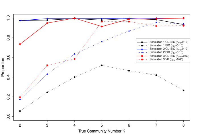
Figure 1: (Color online) Comparisons between different methods for selecting the true community number $K$ in the standard blockmodel settings of Simulations 1 – 3. Along the $y$-axis, we record the proportion of times the chosen number of communities for each of the different criteria for selecting $K$ agrees with the truth.

In addition, Figure 1 presents simulation results where the true community number $K$ increases from $2$ to $8$. Following our previous examples, community sizes grow according to the sequence $(60,90,120,150,60,90,120,150)$. The selected correlation-contaminated stochastic blockmodels are $\rho_{Eq}=0.10$ from Simulation 1, within-community correlation $\rho_{Eq}=0.10$ from Simulation 2, and within-community correlation $\rho_{Dec}=0.60$ from Simulation 3. As $K$ increases and enough vertices are added into the network, CL-BIC tends to correctly estimate the true community number in all simulation settings. Even in this scenario with a growing number of communities, the proportion of times CL-BIC selects the true $K$ is always greater than the corresponding BIC or VB estimates.

Before moving to the last simulation example, we would like to define two measures to quantify the accuracy of a given node label assignment. The first measure is a “goodness-of-fit” (GF) measure defined as

$$\begin{split}GF(\boldsymbol{z},\boldsymbol{\hat{z}_{k}})&=\sum_{i<j}\left(\mathbbm{1}\{z_{i}=z_{j}\}\mathbbm{1}\{\hat{z}_{i}=\hat{z}_{j}\}+\mathbbm{1}\{z_{i}\neq z_{j}\}\mathbbm{1}\{\hat{z}_{i}\neq\hat{z}_{j}\}\right)\Big{/}{N\choose 2},\end{split}$$ (10)

where $\boldsymbol{z}$ represents the true community labels and $\boldsymbol{\hat{z}_{k}}$ represents the community assignments from an estimator. Thus, the measure $GF(\boldsymbol{z},\boldsymbol{\hat{z}_{k}})$ calculates the proportion of pairs whose estimated assignments agree with the correct labels in terms of being assigned to the same or different communities, and is commonly known as the Rand Index (Rand, 1971) in the cluster analysis literature.

The second measure is motivated from the “assortativity” notion. The ratio of the median within community edge number to that of the between community edge number (MR) is defined as

$$MR(\boldsymbol{\hat{z}_{k}})=\operatorname*{median}_{a=1,\ldots,k}\left(m_{aa}\right)\Big{/}\operatorname*{median}_{a\neq b}\left(m_{ab}\right),$$ (11)

where $k$ is the number of communities implied by $\boldsymbol{\hat{z}_{k}}$ and $m_{ab}$ is the total number of edges between communities $a$ and $b$, as given by the community assignment $\boldsymbol{\hat{z}_{k}}$. It is clear that for both measures, a higher value indicates a better community detection performance.

As a final simulation example, we analyze the performance of CL-BIC and BIC for a growing number of communities under the degree-corrected blockmodel. While the reparametrized vector $\boldsymbol{\theta}_{n}=\boldsymbol{\gamma}_{n}\boldsymbol{\theta}$ remains as in Simulation 4, the $\omega_{i}$ are now independently generated from Uniform$(1/5,9/5)$. The results are collected in Table 5, where we also record the performance of the SCORE algorithm under the true $K$, along with the goodness-of-fit (GF) and median ratio (MR) performance measures introduced in (10) and (11), respectively.

Table 5: Comparison of CL-BIC and BIC over $200$ repetitions from the DCBM case in Simulation 4, with $(\rho_{Eq}=0.2,\boldsymbol{\gamma}_{n}=0.03)$, where the individual effect parameters $\omega_{i}$ are now generated from a Uniform$(1/5,9/5)$ distribution.

	SCORE Performance				CL-BIC							BIC
$K$	Misc. R.	Orac. Err.	Est. Err.		PROP	MD	RSD		GF	MR		PROP	MD	RSD	GF	MR
2	0.02	0.51	0.54		0.88	1	0		0.96	7.33		0.10	2	0.75	0.73	3.37
3	0.03	0.53	0.55		0.93	1	0	.75	0.97	7.87		0.09	3	1.49	0.88	3.91
4	0.03	0.55	0.58		0.86	1	0		0.97	8.11		0.16	3	1.49	0.91	5.41
5	0.04	0.58	0.62		0.56	1	0		0.96	6.35		0.09	3	2.05	0.92	5.92
6	0.05	0.60	0.64		0.47	1	1	.49	0.96	7.10		0.09	2	2.24	0.94	7.08
7	0.05	0.63	0.66		0.39	1	1	.49	0.97	6.77		0.09	3	1.49	0.95	6.73
8	0.08	0.63	0.66		0.29	1	1	.49	0.97	7.24		0.02	3	2.24	0.96	6.80

• NOTE: PROP, proportion; MD, median deviation; RSD, robust standard deviation; GF, goodness-of-fit measure; MR: median ratio measure. Misc. R. denotes the misclustering rate of the SCORE algorithm. For $\Omega=E_{\boldsymbol{\theta}}(\boldsymbol{A})$, Orac. Err. and Est. Err. are $\left\lVert\Omega_{O}-\Omega\right\rVert/\left\lVert\Omega\right\rVert$ and $\left\lVert\Omega_{SC}-\Omega\right\rVert/\left\lVert\Omega\right\rVert$, respectively, where $\left\lVert\cdot\right\rVert$ denotes Frobenius norm. Here, $\Omega_{O}$ denotes the estimate of $\Omega$ under the oracle scenario where we know the true community assignment $\boldsymbol{z}\in\{1,\ldots,K\}^{N}$, and $\Omega_{SC}$ is the estimate of $\Omega$ using the SCORE labeling vector.

The true community number and community sizes grow as in the case for the standard blockmodel described in Figure 1. Although CL-BIC performs uniformly better than BIC across all validating criteria and throughout all $K$, the procedure does not appear to yield model selection consistent results in this example. Aside from the fact that the introduced correlation is not exponentially decaying, this poor performance as $K$ increases can also be explained by the difficulty in estimating the DCBM parameters $(\boldsymbol{\theta},\boldsymbol{\omega})$ in a scenario where several vertices have potentially low degrees. Indeed, even in the oracle scenario where we know the true community labels $z_{i}$ ahead of time, and for a relatively small misclustering rate of the SCORE algorithm, Table 5 exhibits the difficulty in obtaining accurate estimates $(\boldsymbol{\hat{\theta}}_{\text{C}},\boldsymbol{\hat{\omega}}_{\text{C}})$, and in evaluating the CL-BIC criterion functions (8), under this increasing $K$ scenario for the DCBM. Whether the increased number of parameters in the DCBM has an effect on the consistency results of CL-BIC as $K$ increases is also an interesting line of future work.

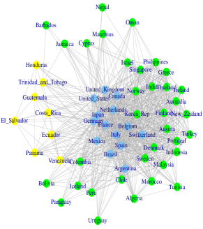
(a) $k=3$ (CL-BIC-SBM)

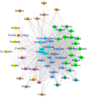
(b) $k=7$ (VB-SBM)

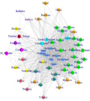
(c) $k=10$ (BIC-SBM)

Figure 2: (Color online) Largest connected component of the international trade network for the year $1995$.

4.2 Real Data Analysis

4.2.1 International Trade Networks

We first study an international trade dataset originally analyzed in Westveld and Hoff (2011), containing yearly international trade data between $N=58$ countries from $1981-2000$. For a more detailed description of this dataset, we refer the interested reader to the Appendix in Westveld and Hoff (2011). In our numerical comparisons between CL-BIC and BIC paired with the standard stochastic blockmodel log-likelihood (1), we focus on data from year 1995. For this network, an adjacency matrix $\boldsymbol{A}$ can be formed by first considering a weight matrix $\boldsymbol{W}$ with $W_{ij}=\text{Trade}_{i,j}+\text{Trade}_{j,i}$, where $\text{Trade}_{i,j}$ denotes the value of exports from country $i$ to country $j$. Finally, we define $A_{ij}=1$ if $W_{ij}\geq W_{\alpha}$, and $A_{ij}=0$ otherwise; here $W_{\alpha}$ denotes the $\alpha$-th quantile of $\{W_{ij}\}_{1\leq i<j\leq N}$. For the choice of $\alpha=0.5$, Figure 2 shows the largest connected component of the resulting network. Panel (a) shows CL-BIC selecting $3$ communities, corresponding to countries with the highest GDPs (dark blue), industrialized European and Asian countries with medium-level GDPs (green), and developing countries in South America with the smallest GDPs (yellow). Next, in panel (b) we also show the variational Bayes solution corresponding to $k=7$, providing finer communities for some Central and South American neighboring countries (yellow and pink, respectively) but fragmenting the high- and medium-level GDP countries into ambiguous communities. For instance, it is not clear why countries like Bolivia and Nepal belong to the same community (orange) or why the Netherlands, rather than Brazil or Italy, joined the community of countries with the highest GDPs (light blue). At last, panel (c) corresponds to the final BIC model selecting $10$ communities. Under this partition, South American countries are now split into $6$ “noisy” communities, while high GDP countries are unnecessarily fragmented into two.

We believe CL-BIC provides a better model than traditional BIC, yielding communities with countries sharing similar GDP values without dividing an entire continent into $6$ smaller communities. On the contrary, BIC selects a model containing communities of size as small as one, which are of little, if any, practical use. The variational Bayes approach provides a meaningful solution in this example, exhibiting a similar performance as in Latouche et al. (2012) in terms of providing some finer community assignments.

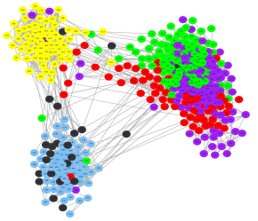
(a) $k=6$ (CL-BIC-DCBM)

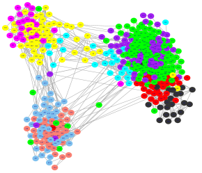
(b) $k=9$ (BIC-DCBM)

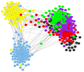
(c) “Truth” $(K=6)$

Figure 3: (Color online) Largest connected component of the school friendship network. Panel (c) shows the “true” grade community labels: $7$th (blue), $8$th (yellow), $9$th (green), $10$th (purple), $11$th (red), and $12$th (black).

4.2.2 School Friendship Networks

Now, we consider a school friendship network obtained from the National Longitudinal Study of Adolescent Health (http://www.cpc.unc.edu/projects/addhealth). For this network, $A_{ij}=1$ if either student $i$ or $j$ reported a close friendship tie between the two, and $A_{ij}=0$ otherwise. We focus on the network of school 7 from this dataset, and our comparisons between CL-BIC and BIC are done with respect to the degree-corrected blockmodel log-likelihood (2). With $433$ vertices, Figure 3 shows the largest connected component of the resulting network. As shown in panel (a), CL-BIC selects the true community number $K=6$, roughly agreeing with the actual grade labels, except for the black community. BIC, shown in panel (b), selects $9$ communities, unnecessarily splitting the $7$th and $8$th graders. The “true” friendship network is shown in panel (c).

We still conclude CL-BIC performs better than traditional BIC. Except for the misallocation of the black community of $12$th graders, the model selected by CL-BIC correctly labels most of the remaining network. While BIC partially separates the 10th graders and the 12th graders, a substantial portion of the 10th graders are absorbed into the 9th grader community (green). In addition, BIC further fragments $7$th and $8$th graders into “noisy” communities. This is an extremely difficult community detection problem since, even for a “correctly” specified $k=6$, SCORE fails to assign all $12$th graders to their corresponding true grade. The black community selected by SCORE in panel (a) mainly corresponds to female students and hispanic males, reflecting perhaps closer friendship ties among a subgroup of students recently starting junior high school.

Using the “goodness-of-fit” measure defined in (10), we found that the CL-BIC community assignment leads to $GF(\boldsymbol{z},\boldsymbol{\hat{z}_{6}})=0.811$, which is slightly better than the $GF(\boldsymbol{z},\boldsymbol{\hat{z}_{9}})=0.810$ obtained for BIC. For the MR measure given in (11), the results for CL-BIC and BIC are $MR(\boldsymbol{\hat{z}_{6}})=40.8$ and $MR(\boldsymbol{\hat{z}_{9}})=33.3$, respectively, again indicating the superiority of the CL-BIC solution paired with SCORE.

In both examples, BIC tends to overestimate the “true” community number $K$, rendering very small communities which are in turn penalized under the CL-BIC approach. This means CL-BIC successfully remedies the robustness issues brought in by spectral clustering, due to the misspecification of the underlying stochastic blockmodels, and effectively captures the loss of variance produced by using traditional BIC.

.   iscussion

There has been a tremendous amount of research in recovering the underlying structures of network data, especially on the community detection problem. Most of the existing work has focused on studying the properties of the stochastic blockmodel and its variants without looking at the possible model misspecification problem. In this paper, under the standard stochastic blockmodel and its variants, we advocate the use of composite likelihood BIC for selecting the number of communities due to its simplicity in implementation and its robustness against correlated binary data.

Some extensions are possible. For instance, the proposed methodology in this work is based on the spectral clustering and SCORE algorithms, and it would be interesting to explore the combination of the CL-BIC with other community detection methods. In addition, most examples considered here are dense graphs, which are common but cannot exhaust all scenarios in real applications. Another open problem is to study whether the CL-BIC approach is consistent for the degree-corrected stochastic blockmodel, which is not necessarily true from our numerical studies.

upplementary Materials

R Code and Trade Dataset:

The R codes can be used to replicate the simulation studies and the real data analysis. The international trade network dataset is also included. More details can be found in the file README contained in the zip file (CLBIC.zip).

cknowledgements

The authors thank the editor, the associate editor, and two anonymous referees for their constructive comments which have greatly improved the paper. Yu is partially supported by Richard Samworth’s Engineering and Physical Sciences Research Council Early Career Fellowship EP/J017213/1. Feng is partially supported by NSF grant DMS-1308566.

References

- Airoldi et al. (2008) Airoldi, E. M., Blei, D. M., Fienberg, S. E., and Xing, E. P. (2008). Mixed membership stochastic blockmodels. Journal of Machine Learning Research, 9:1981–2014.
- Chen and Lei (2014) Chen, K. and Lei, J. (2014). Network cross-validation for determining the number of communities in network data. Available at arXiv:1411.1715v1.
- Choi et al. (2012) Choi, D. S., Wolfe, P. J., and Airoldi, E. M. (2012). Stochastic blockmodels with a growing number of classes. Biometrika, 99:273–284.
- Cox and Reid (2004) Cox, D. R. and Reid, N. (2004). A note on pseudolikelihood constructed from marginal densities. Biometrika, 91:729–737.
- Daudin et al. (2008) Daudin, J.-J., Picard, F., and Robin, S. (2008). A mixture model for random graphs. Statistics and Computing, 18:173–183.
- Decelle et al. (2011) Decelle, A., Krzakala, F., Moore, C., and Zdeborová, L. (2011). Asymptotic analysis of the stochastic block model for modular networks and its algorithmic applications. Physical Review E, 84:066106.
- Donath and Hoffman (1973) Donath, W. E. and Hoffman, A. J. (1973). Lower bounds for the partitioning of graphs. IBM Journal of Research and Development, 17:420–425.
- Fearnhead (2004) Fearnhead, P. (2004). Particle filters for mixture models with an unknown number of components. Statistics and Computing, 14:11–21.
- Ferguson (1973) Ferguson, T. S. (1973). A bayesian analysis of some nonparametric problems. The Annals of Statistics, 1:209–230.
- Gao and Song (2010) Gao, X. and Song, P. X.-K. (2010). Composite likelihood bayesian information criteria for model selection in high-dimensional data. Journal of The American Statistical Association, 105:1531–1540.
- Goldenberg et al. (2010) Goldenberg, A., Zheng, A. X., Fienberg, S. E., and Airoldi, E. M. (2010). A survey of statistical network models. Foundations and Trends in Machine Learning, 2:129–233.
- Guattery and Miller (1998) Guattery, S. and Miller, G. L. (1998). On the quality of spectral separators. SIAM Journal on Matrix Analysis and Applications, 19:701–719.
- Guyon (1995) Guyon, X. (1995). Random Fields on a Network: Modeling, Statistics, and Applications. Springer-Verlag, New York.
- Handcock et al. (2007) Handcock, M. S., Raftery, A. E., and Tantrum, J. M. (2007). Model-based clustering for social networks. Journal of the Royal Statistical Society, Series A, 170:301–354.
- Heagerty and Lele (1998) Heagerty, P. J. and Lele, S. R. (1998). A composite likelihood approach to binary spatial data. Journal of the American Statistical Association, 93:1099–1111.
- Holland et al. (1983) Holland, P. W., Laskey, K. B., and Leinhardt, S. (1983). Stochastic blockmodels: First steps. Social Networks, 5:109–137.
- Hunter et al. (2012) Hunter, D. R., Krivitsky, P. N., and Schweinberger, M. (2012). Computational statistical methods for social network models. Journal of Computational and Graphical Statistics, 21:856–882.
- Jin (2015) Jin, J. (2015). Fast community detection by SCORE. The Annals of Statistics, 43:57–89.
- Karrer and Newman (2011) Karrer, B. and Newman, M. E. J. (2011). Stochastic blockmodels and community structure in networks. Physical Review E, 83:016107.
- Latouche et al. (2012) Latouche, P., Birmelé, E., and Ambroise, C. (2012). Variational Bayesian inference and complexity control for stochastic block models. Statistical Modelling, 12:93–115.
- Leisch et al. (1998) Leisch, F., Weingessel, A., and Hornik, K. (1998). On the generation of correlated artifical binary data. Working Paper Series, SFB, Adaptive Information Systems and Modelling in Economics and Management Science.
- Lindsay (1988) Lindsay, B. G. (1988). Composite likelihood methods. Contemporary Mathematics, 80:221–239.
- McDaid et al. (2013) McDaid, A. F., Murphy, T. B., Friel, N., and Hurley, N. J. (2013). Improved bayesian inference for the stochastic blockmodel with application to large networks. Computational Statistics and Data Analysis, 60:12–31.
- Miller and Harrison (2014) Miller, J. W. and Harrison, M. T. (2014). Inconsistency of pitman-yor process mixtures for the number of components. Journal of Machine Learning Research, 15:3333–3370.
- Minka (2000) Minka, T. P. (2000). Estimating a dirichlet distribution. Technical report, Microsoft Research.
- Newman (2004) Newman, M. E. J. (2004). Detecting community structure in networks. The European Physical Journal B, 38:321–330.
- Newman and Girvan (2004) Newman, M. E. J. and Girvan, M. (2004). Finding and evaluating community structure in networks. Physical Review E, 69:026113.
- Nobile and Fearnside (2007) Nobile, A. and Fearnside, A. (2007). Bayesian finite mixtures with an unknown number of components: The allocation sampler. Statistics and Computing, 17:147–162.
- Perry and Wolfe (2012) Perry, P. O. and Wolfe, P. J. (2012). Null models for network data. Available at arXiv:1201.5871v1.
- Rand (1971) Rand, W. M. (1971). Objective criteria for the evaluation of clustering methods. Journal of the American Statistical Association, 66:846–850.
- Rohe et al. (2011) Rohe, K., Chatterjee, S., and Yu, B. (2011). Spectral clustering and the high-dimensional stochastic blockmodel. The Annals of Statistics, 39:1878–1915.
- Rohe et al. (2014) Rohe, K., Qin, T., and Fan, H. (2014). The highest dimensional stochastic blockmodel with a regularized estimator. Statistica Sinica, 24:1771–1786.
- Schweinberger and Handcock (2015) Schweinberger, M. and Handcock, M. S. (2015). Local dependence in random graph models: characterization, properties and statistical inference. Journal of the Royal Statistical Society, Series B, 77:647–676.
- Shi and Malik (2000) Shi, J. and Malik, J. (2000). Normalized cuts and image segmentation. IEEE Transactions on Pattern Analysis and Machine Intelligence, 22:888–905.
- Spielmat and Teng (1996) Spielmat, D. A. and Teng, S.-H. (1996). Planar graphs and finite element meshes. In Foundations of Computer Science, 1996. Proceedings., 37th Annual Symposium on, pages 96–105. IEEE.
- Stephens (2000) Stephens, M. (2000). Bayesian analysis of mixture models with an unknown number of components - an alternative to reversible jump methods. The Annals of Statistics, 28:40–74.
- Varin (2008) Varin, C. (2008). On composite marginal likelihoods. AStA Advances in Statistical Analysis, 92:1–28.
- Varin et al. (2011) Varin, C., Reid, N., and Firth, D. (2011). An overview of composite likelihood methods. Statistica Sinica, 21:5–42.
- Varin and Vidoni (2005) Varin, C. and Vidoni, P. (2005). A note on composite likelihood inference and model selection. Biometrika, 92:519–528.
- von Luxburg (2007) von Luxburg, U. (2007). A tutorial on spectral clustering. Statistics and Computing, 17:395–416.
- Wei and Cheng (1989) Wei, Y.-C. and Cheng, C.-K. (1989). Towards efficient hierarchical designs by ratio cut partitioning. In Computer-Aided Design, 1989. ICCAD-89. Digest of Technical Papers., 1989 IEEE International Conference on, pages 298–301.
- Westveld and Hoff (2011) Westveld, A. H. and Hoff, P. D. (2011). A mixed effects model for longitudinal relational and network data, with applications to international trade and conflict. The Annals of Applied Statistics, 5:843–872.
- Zhao et al. (2012) Zhao, Y., Levina, E., and Zhu, J. (2012). Consistency of community detection in networks under degree-corrected stochastic block models. The Annals of Statistics, 40:2266–2292.