A Bayesian hierarchical spatial point process model for multi-type neuroimaging meta-analysis

Abstract

Neuroimaging meta-analysis is an important tool for finding consistent effects over studies that each usually have 20 or fewer subjects. Interest in meta-analysis in brain mapping is also driven by a recent focus on so-called “reverse inference”: where as traditional “forward inference” identifies the regions of the brain involved in a task, a reverse inference identifies the cognitive processes that a task engages. Such reverse inferences, however, require a set of meta-analysis, one for each possible cognitive domain. However, existing methods for neuroimaging meta-analysis have significant limitations. Commonly used methods for neuroimaging meta-analysis are not model based, do not provide interpretable parameter estimates, and only produce null hypothesis inferences; further, they are generally designed for a single group of studies and cannot produce reverse inferences. In this work we address these limitations by adopting a nonparametric Bayesian approach for meta-analysis data from multiple classes or types of studies. In particular, foci from each type of study are modeled as a cluster process driven by a random intensity function that is modeled as a kernel convolution of a gamma random field. The type-specific gamma random fields are linked and modeled as a realization of a common gamma random field, shared by all types, that induces correlation between study types and mimics the behavior of a univariate mixed effects model. We illustrate our model on simulation studies and a meta-analysis of five emotions from 219 studies and check model fit by a posterior predictive assessment. In addition, we implement reverse inference by using the model to predict study type from a newly presented study. We evaluate this predictive performance via leave-one-out cross-validation that is efficiently implemented using importance sampling techniques.

FLA

, ,
and T1Supported by the NIH Grant 5-R01-NS-075066 (TDJ, TEN, TDW), the United Kingdom’s Medical Research Council Grant G0900908 (TEN) and the Welcome Trust (TEN). The work presented in this manuscript represents the views of the authors and not necessarily that of the NIH, UKMRC or the Welcome Trust.

1 Introduction

Functional neuroimaging has experienced rapid growth since the early nineties when Functional Magnetic Resonance Imaging (fMRI) was developed. As the number of studies has grown exponentially, for example, from two fMRI studies in 1993 to over 2600 in 2012, neuroscientists are increasingly interested in formal synthesis of findings across studies via meta-analysis [Yarkoni et al. (2010)]. A neuroimaging meta-analysis mitigates the problems of a single functional neuroimaging study. For example, most neuroimaging studies have relatively low power due to small sample size. For example, a recent meta-analysis of 90 neuroimaging studies on emotion found that the median sample size was a mere 13 subjects [Lindquist et al. (2012)]. Meta-analysis increases statistical power by combining results from several smaller studies. Another problem is that many published fMRI studies use ad hoc significance thresholds that result in high false positive rates and idiosyncratic findings. Thus the principal motivations for neuroimaging meta-analysis are to increase statistical power and to find consistent activation regions across studies, making it possible to separate reproducible findings from idiosyncratic ones.

Another important motivation for meta-analysis is the recent interest in “reverse inference” [Poldrack (2011)]. A traditional fMRI analysis conditions on the task paradigm and produces a “forward inference”, identifying the brain regions involved in the task. The cognitive scientist will then display this set of brain regions and argue, qualitatively, that this is evidence that the task produced a particular cognitive state. However, the resulting brain regions may be nonspecific and in fact activated by a range of cognitive tasks. In one particularly egregious example [Iacoboni et al. (2007)], a neuro-politics study inferred that brain activity in the anterior cingulate, induced by images of Hillary Clinton, indicated that subjects were experiencing emotional conflict; in fact, the anterior cingulate is the most commonly active brain region, found in about 20% of all studies [Yarkoni et al. (2011)] that range from working memory to decision making, as well as emotional processing. Hence there is great interest in using predictive analyses to estimate, conditional on brain activation map, the most likely class of task paradigms that gave rise to the data. This process, referred to as reverse inference, requires a set of meta-analyses, one for each class of task paradigms. Reverse inference can also be used to test the validity of the definition of task categories. That is, if studies can be reliably classified between fine subdivisions of a task type, this is evidence that the subdivisions are typified by unique patterns brain activity and are not arbitrary constructs.

The information that is routinely reported in the literature, and thus available for a meta-analysis, are the spatial locations of local maxima of statistic values within each region of significant activation. These locations are referred to as peak activation locations, or foci. Functional neuroimaging meta-analysis studies based on these foci are called coordinate based meta-analysis (CBMA). Many CBMA methods have been proposed, including Fox et al. (1997), Nielsen and Hansen (2002), Turkeltaub et al. (2002), Wager, Jonides and Reading (2004), Kober et al. (2008), Eickhoff et al. (2009), Radua and Mataix-Cols (2009), Kang et al. (2011) and Yue, Lindquist and Loh (2012). To date, the most widely used methods are kernel based methods including activation likelihood estimation [Turkeltaub et al. (2002), ALE], modified ALE [Eickhoff et al. (2009), modALE] and multilevel kernel density analysis [Kober et al. (2008), MKDA]. However, these methods have serious limitations. First, they require ad hoc spatial kernel parameters, which must be pre-specified in the analysis. Second, ALE maps are difficult to interpret, as they are couched in probabilistic terminology but are not actually based on a formal statistical model. Third, they are based on a massive univariate approach that lacks an explicit spatial model. Thus, these methods can only detect effects that consistently overlap in space, and cannot assess spatial variability inherent in the foci.

To address these deficiencies Kang et al. (2011) proposed a Bayesian hierarchical independent cluster process (BHICP) model. This model is for a single class of studies, and does not accommodate the multi-type point processes needed for reverse inference. While BHICP model could be extended there are three significant limitations: (1) the model involves many hyperprior distributions whose parameters are challenging to elicit; (2) the posterior intensity function is somewhat sensitive to the choice of hyperpriors; and (3) the parametric form of the clustering may not be appropriate for all types of spatial patterns found in CBMA data. Although it is possible to extend this model by adding another level to the hierarchy, doing so would only compound these problems.

More recently, Yue, Lindquist and Loh (2012) proposed a Bayesian spatial generalized linear model (SGLM) that treats the CBMA data as binary random variables, one at each voxel. See Yue, Lindquist and Loh (2012) for details. There are several limitations to this approach as well. First, this approach does not treat the individual studies as the units of observation, but instead assumes the data at each voxel are the units of observation. Second, the structure of CBMA data implies that the number and locations of the foci within each study is random and this approach does not respect this structure. Third, it is not a generative, or predictive, model. While this SGLM approach does have its merits, in this article we adopt the spatial point process approach. The spatial point process approach more accurately captures the stochastic structure of the data. Specifically that one unit of data is an individual study comprised of a random number of foci occurring at random locations.

Although many parametric spatial point process models have been proposed for the analysis of multi-type point patterns [Møller and Waagepetersen (2004)] any specific parametric intensity function is difficult to justify. Therefore, we propose a nonparametric Bayesian model to fit multi-type (emotion) meta-analyses by extending the Poisson/gamma random field (PGRF) model developed by Wolpert and Ickstadt (1998a) to a hierarchical PGRF (HPGRF) model. The PGRF model is a Cox process [Cox (1955)] in which the intensity function is modeled nonparametrically as the convolution of a spatial kernel and a gamma random field. This model has found widespread use due to its robustness in intensity function estimation and its computational efficiency [Ickstadt and Wolpert (1999), Best, Ickstadt and Wolpert (2000), Best et al. (2002), Stoyan and Penttinen (2000), Niemi and Fernández (2010), Woodard, Wolpert and O’Connell (2010)]. Our generalization from the PGRF model to the HPGRF model is analogous to the extension of the mixture of Dirichlet process priors model to the hierarchical mixture of Dirichlet process priors model [Teh et al. (2006)]. In particular, we consider each type of spatial point pattern as a realization of a PGRF model where the gamma random field for each type is a realization from a population level gamma random field (hence the hierarchy or “random effects”). The random intensity functions for the different types are related, thus allowing not only aggregation of points within a type, but aggregation of points across types. The proposed HPGRF model has the following advantages over the BHICP model: (1) It is a nonparametric model which provides more flexibility in estimating the intensity function (which is also an advantage over other spatial point process models such as the log-Gaussian Cox process and Markov random field models [Møller and Waagepetersen (2004)]). (2) It requires fewer hyperparameters and is less sensitive to the prior specification. (3) It jointly estimates multi-type point patterns, borrowing strength across the subtypes.

Our motivating data set comes from a functional neuroimaging meta-analysis of emotions [Kober et al. (2008)]. Kober et al. collected data from 219 functional neuroimaging studies on five emotions (sad, happy, anger fear and disgust). We will use reverse inference to assess evidence for one perspective on emotional regulation. The “constructionist view” [Lindquist et al. (2012)] suggests that the basic categories of emotion (fear, disgust, etc.) arise from complex combinations of elemental information-processing operations across the brain. By this view, regions like the amygdala might be involved in all of the basic emotions, but to different degrees with other areas depending on the emotion type. Thus, the constructionist theory suggests that a hierarchical model, or “random effects” type of model, is appropriate. Thus, the BHICP and the PGRF models are not applicable as they only model a single emotion type. In particular, neither approach can borrow strength, nor model correlation, across the different emotions as suggested by the constructionist view.

The remainder of this article is organized as follows. In Section 2, we present our HPGRF model for multi-type point patterns. We outline the model in Section 2.2. In Section 2.3 we provide a theorem detailing the expectation and covariance of the associated counting process within a sub-type and the covariance of the counting processes between subtypes for any two regions of interest in the sampling window. In Section 2.4 we present a data augmentation scheme and in Section 2.5 we present an inverse Lévy measure representation of the augmented model. We assess model performance via simulation studies in Section 3 and analyze the emotions meta-analysis data set in Section 4. We conclude with a brief discussion in Section 5.

2 The model

In this section, we start with a short overview of spatial point processes, which are very useful tools in the analysis of spatial point patterns [Møller and Waagepetersen (2004)], then introduce our HPGRF model for multi-type spatial point patterns motivated by the meta-analysis of functional neuroimaging data. In this article, all the point patterns are defined on $\mathcal{B}\subset\mathbb{R}^{3}$ where $\mathcal{B}$ represents the human brain.

2.1 Spatial point processes

For our purposes, a spatial point process $\mathbf{Y}$ is a random countable subset on the brain, $\mathcal{B}$. For a spatial point process, there is an associated counting process, $N_{\mathbf{Y}}(A)$, that counts the number of points of $\mathbf{Y}$ in (well-behaved) subsets $A\subseteq\mathcal{B}$. One of the most important spatial point processes is the Poisson point process. A Poisson point process is characterized by an intensity function: a nonnegative function that is integrable on all bounded subsets of $\mathcal{B}$. Since the brain is a bounded subset of $\mathbb{R}^{3}$, for our purposes, integrability on $\mathcal{B}$ is sufficient. We will use $\lambda(y)$, $y\in\mathcal{B}$, to denote the intensity function. A spatial point process is a Poisson point process if and only if (1) for all $A\subseteq\mathcal{B}$, $N_{\mathbf{Y}}(A)$ follows a Poisson distribution with mean $\Lambda(A)=\int_{A}\lambda(y)\,dy$, and (2) conditional on $N_{\mathbf{Y}}(A)=n$, all points in $\mathbf{Y}$, that is, $y_{1},\ldots,y_{n}$, are independent and identically distributed with density $\lambda(y)/\Lambda(\mathcal{B})$.

The intensity function in a Poisson point process is a known deterministic function. This limits its use and flexibility in modeling data. Thus, Cox (1955) introduced the doubly stochastic Poisson process; commonly known now as the Cox process. The Cox process generalizes the Poisson point process by allow the intensity function to be a random intensity function. Suppose now that $\lambda(y)$ is a random, nonnegative function that is integrable on $\mathcal{B}$. If, conditional on $\lambda(y)$, the point process $\mathbf{Y}$ is a Poisson point process, then marginally, $\mathbf{Y}$ is said to be a Cox process driven by $\lambda$.

Many Cox processes have been introduced in the literature with various modeling assumptions on the random intensity function, $\lambda$. Most of these assume that $\lambda$ is a parametrized function. For example, the log-Gaussian Cox process [Møller, Syversveen and Waagepetersen (1998)] assumes $\ln[\lambda(y)]=U(y)$ where $U(y)$ is a Gaussian process parametrized by a mean, a marginal variance and a correlation function (also parametrized). There is a vast literature on spatial point processes. We refer the interested reader to but a few: Illian et al. (2008), Møller and Waagepetersen (2007) and van Lieshout and Baddeley (2002).

As a nonparametric alternative to these parametric intensity functions, Wolpert and Ickstadt (1998a) proposed the Poisson/gamma random field (PGRF) model. They model the random intensity function as a convolution of a finite kernel, $k_{\sigma^{2}}(\mathrm{y},\mathrm{x})$, and a gamma random field, $G(d\mathrm{x})$: $\lambda(y)=\int_{\mathcal{B}}k_{\sigma^{2}}(\mathrm{y},\mathrm{x})G(d\mathrm{x})$, where $\sigma^{2}$ is the kernel variance. As an example, consider Figure 1. In panel (A), we show the jump locations and the jump heights from a simulated gamma random field on the unit square. In panel (B), we show the intensity function produced by the convolution of a Gaussian kernel with the gamma random field from panel (A). Panel (C) shows the intensity function as an image with the points representing a single realization of a point pattern drawn from this PGRF. Note the distinctly non-Gaussian shapes in panels (B) and (C), although the intensity function is modeled with a Gaussian kernel.

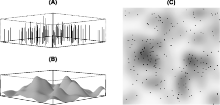
Figure 1: A simulated two-dimensional gamma random field [jump heights, panel (A)], the corresponding intensity function [convolution with a kernel, panel (B)] and one realization of the PGRF [panel (C)].

A gamma random field is characterized by a base measure $a(d\mathrm{x})$ and an inverse scale parameter $b$. If the random field $G(dx)$ is gamma random field, we denote this by $G(dx)\sim\mathcal{GRF}\{a(d\mathrm{x}),b\}$. The gamma process (or random field) was first defined by Ferguson (1973). Formally, if a random field $G(d\mathrm{x})\sim\mathcal{GRF}\{a(d\mathrm{x}),b\}$, then for any partition of the space $\mathcal{B}$, $\{A_{k}\}_{k=1}^{K}$ (i.e., $\mathcal{B}=\bigcup_{k=1}^{K}A_{k}$ and $A_{k}\cap A_{j}=\varnothing$ for $k\neq j$), $G(A_{1}),\ldots,G(A_{K})$ are mutually independent and $G(A_{k})$ follows a gamma distribution with shape $a(A_{k})$ and inverse scale $b$. Wolpert and Ickstadt (1998a, b) provide a construction of a gamma random field that highlights the nonparametric nature of the process (see, also, Section 2.5).

In this article, we assume that both $k_{\sigma^{2}}(\mathrm{y},\mathrm{x})$ and $\lambda(\mathrm{y})$ are Lebesgue measurable functions. We define $K_{\sigma^{2}}(B,\mathrm{x})=\int_{B}k_{\sigma^{2}}(\mathrm{y},\mathrm{x})\ell(d\mathrm{y})$ and $\Lambda(B)=\int_{B}\lambda(\mathrm{y})\ell(d\mathrm{y})$ for any Lebesgue measurable set $B\subseteq\mathcal{B}$, where $\ell$ is Lebesgue measure. $K_{\sigma^{2}}(\cdot,\mathrm{x})$ is called a kernel measure whereas $\Lambda(\cdot)$ is called an intensity measure. We can choose $k_{\sigma^{2}}(\mathrm{y},\mathrm{x})$ to be a probability density function on $\mathcal{B}$. Thus, we have $\Lambda(d\mathrm{y})=\int_{\mathcal{B}}K_{\sigma^{2}}(d\mathrm{y},\mathrm{x})G(d\mathrm{x})$. The PGRF model has been successful in the analysis of a single realization of a point pattern, which is typical for most point pattern data. This model enjoys most key advantages of parametric models, but can accommodate irregular shapes of point clusters, is more flexible, and adaptive to data.

Before we introduce our model, one point of notation is in order. A spatial Poisson point process is defined by specifying the sampling window of interest (the brain, $\mathcal{B}$, in our case) and either an intensity function or, equivalently, the associated intensity measure. Both the intensity function and intensity measure carry the same information about the process. We choose the latter to be consistent with Wolpert and Ickstadt (1998a). Thus, if $\mathbf{Y}$ is a Poisson point process on $\mathcal{B}$ with intensity measure $\Lambda$, we denote this as $\mathbf{Y}\sim\mathcal{PP}\{\mathcal{B},\Lambda(d\mathrm{y})\}$ where the differential $d\mathrm{y}$ is an infinitesimally small volume element in $\mathcal{B}$.

2.2 Hierarchical Poisson/Gamma random fields

In this section, we generalize the PGRF model of Wolpert and Ickstadt (1998a) to model multi-type spatial point pattern with between-type clustering or aggregation. For each emotion, the foci reported from different studies are considered to be spatial point patterns. Each spatial point pattern from each study, for a particular emotion, is assumed to be an independent realization of a spatial point process, where the spatial point processes underlying the different emotions are dependent. We include this dependence between emotions as it is suggested by the constructionist theory of emotion processing. We model the dependence of different emotion-specific spatial point processes using hierarchical gamma random fields.

Let $J$ denote the distinct emotion types studied and let $n_{j}$ denote the number of independent studies of emotion $j$, $j=1,\ldots,J$. Let ${\mathbf{y}}_{i,j}$, $i=1,\ldots,n_{j}$, denote the set of observed foci from study $i$ of emotion $j$ and assume that each ${\mathbf{y}}_{i,j}$ is a realization from a Cox process, $\mathbf{Y}_{i,j}$, driven by a common random intensity measure: $\Lambda_{j}(d\mathrm{y})=\int_{\mathcal{B}}K_{\sigma^{2}_{j}}(d\mathrm{y},\mathrm{x})G_{j}(d\mathrm{x})$, where the $G_{j}(d\mathrm{x})$ are independent and identically distributed with common base measure $G_{0}(d\mathrm{x})$ and inverse scale parameter $\tau$. To introduce dependence between types, we define $G_{0}(d\mathrm{x})$ to be a gamma random field with base measure $\alpha(d\mathrm{x})$ and inverse scale parameter $\beta$. In summary, our model is, for $i=1,\ldots,n_{j},j=1,\ldots,J$,

$$\bigl{[}\mathbf{Y}_{i,j}|\sigma_{j}^{2},G_{j}(dx)\bigr{]} \stackrel{{\scriptstyle\mathrm{i.i.d.}}}{{\sim}} \mathcal{PP}\biggl{\{}\mathcal{B},\int_{\mathcal{B}}K_{\sigma^{2}_{j}}(d\mathrm{y},\mathrm{x})G_{j}(d\mathrm{x})\biggr{\}},$$

$$\bigl{[}G_{j}(d\mathrm{x})|G_{0}(d\mathrm{x}),\tau\bigr{]} \stackrel{{\scriptstyle\mathrm{i.i.d.}}}{{\sim}} \mathcal{GRF}\bigl{\{}G_{0}(d\mathrm{x}),\tau\bigr{\}},$$ (1)

$$\bigl{[}G_{0}(d\mathrm{x})|\alpha(d\mathrm{x}),\beta\bigr{]} \sim \mathcal{GRF}\bigl{\{}\alpha(d\mathrm{x}),\beta\bigr{\}},$$

where the kernel variances, $\sigma_{j}^{2}$, base measure $\alpha(d\mathrm{x})$ and inverse scale parameters $\tau$ and $\beta$, are all given hyperprior distributions that we define later. Note that there are only four parameters in this model—far fewer than the BHICP model. We note here that the HPGRF generalizes the PGRF model of Wolpert and Ickstadt (1998a) in two ways. The first is trivial: we have multiple observations of each emotion type. The second is trivial to introduce, but is nontrivial algorithmically: we introduce another level in the hierarchy. Thus, if we attempt to fit the PGRF model to multi-type point patterns, then necessarily the multi-type patterns are independent of one another. On the contrary, if we fit the HPGRF model to multi-type point patterns, then the multi-type patterns are dependent, as we now demonstrate.

2.3 First and second moment properties

The HPGRF induces spatial correlation between the number of points in any two regions of interest both within an emotion and between emotions. This is an important aspect of our model for the emotion meta-analysis data set and we will show in the simulation study section that when there is aggregation of points between types that there is a gain in efficiency as measured by the mean squared error. We stress the point that by introducing this dependence between intensity functions for the different emotions we take into account the positive dependence (aggregation of points) between emotions offered by the constructionist view of emotion processing. On the other hand, if a repulsive process between emotion types is suggested, this model would not be appropriate.

The conditional mean and covariance structure of $N_{\mathbf{Y}_{j}}(A)$ for the HPGRF model are summarized in the following theorem whose proof is given in Section 1 in the Web Supplementary Material [Kang et al. (2014)].

Theorem 1.

Within emotion type $j$ and for all $A,B\subseteq\mathcal{B}$,

$$\mathrm{E}\bigl{\{}N_{\mathbf{Y}_{j}}(A)|\sigma^{2}_{j},\tau,\alpha,\beta\bigr{\}}=\frac{1}{\tau\beta}\int_{\mathcal{B}}K_{\sigma^{2}_{j}}(A,\mathrm{x})\alpha(d\mathrm{x}),$$

$$\operatorname{Cov}\bigl{\{}N_{\mathbf{Y}_{j}}(A),N_{\mathbf{Y}_{j}}(B)|\sigma^{2}_{j},\tau,\alpha,\beta\bigr{\}}$$

$$\qquad=\frac{1}{\tau\beta}\int_{\mathcal{B}}K_{\sigma^{2}_{j}}(A\cap B,\mathrm{x})\alpha(d\mathrm{x})+\frac{1+\beta}{\tau^{2}\beta^{2}}\int_{\mathcal{B}}K_{\sigma^{2}_{j}}(A,\mathrm{x})K_{\sigma^{2}_{j}}(B,\mathrm{x})\alpha(d\mathrm{x}).$$

Between emotion types $j$ and $k$ ($j\neq k$),

$$\operatorname{Cov}\bigl{\{}N_{\mathbf{Y}_{j}}(A),N_{\mathbf{Y}_{k}}(B)|\sigma^{2}_{j},\sigma^{2}_{k},\tau,\alpha,\beta\bigr{\}}$$

(3)

$$\qquad=\frac{1}{\tau^{2}\beta^{2}}\int_{\mathcal{B}}K_{\sigma^{2}_{j}}(A,\mathrm{x})K_{\sigma^{2}_{k}}(B,\mathrm{x})\alpha(d\mathrm{x}).$$

This theorem shows that, as an a priori property, the intra-emotion and inter-emotion number of points in $A$ and $B$ are positively correlated, regardless of whether $A$ and $B$ are disjoint. When $\sigma^{2}_{j}=\sigma^{2}_{k}$, $j\neq k$, (1) and (1) show that the intra-emotion covariance is larger than the inter-emotion covariance. Posterior inference of the HPGRF model is realized by the following model representation.

2.4 Data augmentation and complete data model

Wolpert and Ickstadt (1998a) propose an alternative model representation based on data augmentation that results in an efficient MCMC algorithm for posterior estimation of the PGRF model. In this section and the next, we generalize their approach to our hierarchical model. First, we attach a mark to each point in $\mathbf{Y}_{j}$. Given our model (2.2), $N_{\mathbf{Y}_{j}}(\mathcal{B})$ is a Poisson random variable with mean $\Lambda_{j}(\mathcal{B})$ and conditional on $N_{\mathbf{Y}_{j}}(\mathcal{B})$, $G_{j}(d\mathrm{y})$ and $\sigma^{2}_{j}$, all points $Y_{j}\in\mathbf{Y}_{j}$ are independent and identically distributed as

$$\bigl{[}Y_{j}|N_{\mathbf{Y}_{j}}(\mathcal{B}),G_{j}(d\mathrm{y}),\sigma^{2}_{j}\bigr{]} \stackrel{{\scriptstyle\mathrm{i.i.d.}}}{{\sim}} \Lambda_{j}(d\mathrm{y})/\Lambda_{j}(\mathcal{B})$$

$$= \biggl{(}\int_{\mathcal{B}}K_{\sigma^{2}_{j}}(d\mathrm{y},\mathrm{x})G_{j}(d\mathrm{x})\biggr{)}\Big{/}\Lambda_{j}(\mathcal{B}).$$

Next, for each $Y_{j}\in\mathbf{Y}_{j}$, we resolve this mixture distribution by drawing an auxiliary random variable $X_{j}=\mathrm{x}_{j}\in\mathcal{B}$ from the distribution,

$$\bigl{[}X_{j}|Y_{j}=y_{j},N_{\mathbf{Y}_{j}}(\mathcal{B}),G_{j}(d\mathrm{x}),\sigma^{2}_{j}\bigr{]}\sim k_{\sigma^{2}_{j}}(y_{j},\mathrm{x})G_{j}(d\mathrm{x})/\lambda_{j}(y_{j}),$$

where $\lambda_{j}(\mathrm{y})$ is the intensity function of spatial point process $\mathbf{Y}_{j}$. Lastly, define $(\mathbf{Y}_{j},\mathbf{X}_{j})=\{(Y_{j},X_{j}),Y_{j}\in\mathbf{Y}_{j}\}$. Then it is easy to show that $(\mathbf{Y}_{j},\mathbf{X}_{j})$ is a Poisson point process on $\mathcal{B}\times\mathcal{B}$ with intensity measure $K_{\sigma^{2}_{j}}(d\mathrm{y},\mathrm{x})G_{j}(d\mathrm{x})$:

$$\bigl{[}(\mathbf{Y}_{j},\mathbf{X}_{j})|K_{\sigma^{2}_{j}}(d\mathrm{y},\mathrm{x})G_{j}(d\mathrm{x})\bigr{]}\sim\mathcal{PP}\bigl{\{}\mathcal{B}\times\mathcal{B},K_{\sigma^{2}_{j}}(d\mathrm{y},\mathrm{x})G_{j}(d\mathrm{x})\bigr{\}}.$$ (4)

By integrating out $\mathbf{X}_{j}$, we recover the distribution of $\mathbf{Y}_{j}$ in (2.2). It is the model in equation (4) that we use in our posterior simulation which is based on the following construction of a gamma random field.

2.5 The Lévy measure construction

Several methods have been proposed to simulate gamma random fields including Bondesson (1982), Damien, Laud and Smith (1995) and Wolpert and Ickstadt (1998b). The inverse Lévy measure algorithm [Wolpert and Ickstadt (1998a, 1998b)] provides an efficient approach that has been successfully applied to the PGRF model. We represent the algorithm in the following theorem.

Theorem 2.

Let $\theta_{m}\stackrel{{\scriptstyle\mathrm{i.i.d.}}}{{\sim}}\widetilde{\alpha}(d\mathrm{x})\equiv\alpha(d\mathrm{x})/\alpha(\mathcal{B})$, $\nu_{m}=E_{1}^{-1}\{\zeta_{m}/\alpha^{\prime}(\theta_{m})\}/\beta$, and $\zeta_{m}=\sum_{l=1}^{m}e_{l}$, for $m=1,2,\ldots,$ where $e_{l}\stackrel{{\scriptstyle\mathrm{i.i.d.}}}{{\sim}}\operatorname{Exp}(1)$, that is, thestandard exponential distribution, and $E_{1}(t)=\int_{t}^{\infty}e^{-u}u^{-1}\,du$. Let $\Gamma(d\mathrm{x})=\break\sum_{m=1}^{\infty}\nu_{m}\delta_{\theta_{m}}(d\mathrm{x})$, then

$$\Gamma(d\mathrm{x})\sim\mathcal{GRF}\bigl{\{}\alpha(d\mathrm{x}),\beta\bigr{\}}.$$

If $\widetilde{\alpha}(d\mathrm{x})=\widetilde{\alpha}^{\prime}(\mathrm{x})\ell(d\mathrm{x})$, then the joint distribution of $\{(\theta_{m},\nu_{m})\}_{m=1}^{M}$ has a density with respect to $\prod_{m=1}^{M}\ell(d\theta_{m})\ell(d\nu_{m})$ proportional to

$$\exp\bigl{\{}-E_{1}(\beta\nu_{M})\widetilde{\alpha}^{\prime}(\theta_{M})\bigr{\}}\prod_{m=1}^{M}\bigl{[}\nu_{m}^{-1}\exp\{-\nu_{m}\beta\}\widetilde{\alpha}^{\prime}(\theta_{m})\bigr{]}.$$

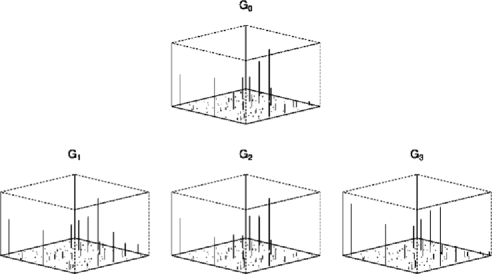
Figure 2: Simulated two-dimensional hierarchical gamma random fields, where $G_{0}$ is the population level gamma random field and $G_{j}$ for $j=1,2,3$ is the individual gamma random field. $G_{0}$ and all the $G_{j}$’s share the same support with different jump heights. On average the jump heights of $G_{j}$ is about those of $G_{0}$.

Note that $\widetilde{\alpha}(d\mathrm{x})$ is a probability measure obtained by normalizing $\alpha(d\mathrm{x})$. The sequence $\{\zeta_{m}\}_{m=1}^{M}$ denotes the arrival times of the standard Poisson process on $\mathbb{R}^{+}$. The $\theta_{m}$ are the jump locations of the gamma random field while $\nu_{m}$ is the jump height at location $\theta_{m}$. This is Theorem 1 and Corollary 2 of Wolpert and Ickstadt (1998a) who also provide a proof. Theorem 2 not only provides an efficient approach to simulate from a gamma random field, it also provides an alternative representation of a gamma random field that simplifies posterior simulation. From this point forward, our Lévy measure construction generalizes that of Wolpert and Ickstadt (1998a) to Hierarchical Poisson/Gamma random fields. Let InvLévy$[\alpha(d\mathrm{x}),\beta]$ represent the joint distribution of $\{(\theta_{m},\nu_{m})\}_{m=1}^{\infty}$ given the base measure $\alpha(d\mathrm{x})$ and inverse scale parameter $\beta$. According to Theorem 2, we can write:

$$G_{0}(d\mathrm{x})=\sum_{m=1}^{\infty}\nu_{m}\delta_{\theta_{m}}(d\mathrm{x}),$$ (5)

where $\{(\theta_{m},\nu_{m})\}_{m=1}^{\infty}\sim\mbox{InvL\'{e}vy}\{\alpha(d\mathrm{x}),\beta\}$. Note that $G_{0}$ has support on $\{\theta_{m}\}_{m=1}^{\infty}$. This implies that each $G_{j}$ necessarily has the same support. See Figure 2 for an illustration. Thus, there exist positive random numbers $\mu_{j,m},j=1,\ldots,J$, such that

$$G_{j}(d\mathrm{x})=\sum_{m=1}^{\infty}\mu_{j,m}\delta_{\theta_{m}}(d\mathrm{x}).$$ (6)

Let $(B_{1},\ldots,B_{r})$ be any finite measurable partition of $\mathcal{B}$. Let $A_{l}=\{m\dvtx\theta_{m}\in B_{l}\}$ for $l=1,\ldots,r$. This implies that $(A_{1},\ldots,A_{r})$ is a finite partition of the natural numbers. For each $j$ and $l$, we have $G_{j}(B_{l})\sim\operatorname{Gamma}(G_{0}(B_{l}),\tau)$ so that $\sum_{m\in A_{l}}\mu_{j,m}\sim\operatorname{Gamma}(\sum_{m\in A_{l}}\nu_{m},\tau)$. Thus, for $m=1,2,\ldots,$

$$\mu_{j,m}\sim\operatorname{Gamma}(\nu_{m},\tau).$$ (7)

We note here that the $\mu_{j,m}$ are the jump heights of the gamma random field $G_{j}(dx)$ and can be thought of as random effects about the population level jump heights $\nu_{m}$ scaled by $\tau$. That is, $E(\mu_{j,m})=\nu_{m}/\tau$. Finally, combining equations (4), (5), (6) and (7) we have the following equivalent representation of our HPGRF model:

$$\bigl{[}(\mathbf{Y}_{j},\mathbf{X}_{j})|\bigl{\{}(\mu_{j,m},\theta_{m})\bigr{\}}_{m=1}^{\infty},\sigma^{2}_{j}\bigr{]}$$

$$\qquad\sim\mathcal{PP}\Biggl{\{}\mathcal{B}\times\mathcal{B},K_{\sigma^{2}_{j}}(d\mathrm{y},\mathrm{x})\sum_{m=1}^{\infty}\mu_{j,m}\delta_{\theta_{m}}(d\mathrm{x})\Biggr{\}},$$

(8)

$$[\mu_{j,m}|\nu_{m},\tau]\stackrel{{\scriptstyle\mathrm{i.i.d.}}}{{\sim}}\operatorname{Gamma}(\nu_{m},\tau),$$

$$\bigl{\{}(\theta_{m},\nu_{m})\bigr{\}}_{m=1}^{\infty}\sim\mbox{InvL\'{e}vy}\bigl{\{}\alpha(d\mathrm{x}),\beta\bigr{\}}.$$

In practice, we cannot sample $\{(\mathbf{Y}_{j},\mathbf{X}_{j})\}_{j=1}^{J}$ according to (2.5), since it requires simulating an infinite number of parameters which, in fact, reflects the nonparametric nature of both the PGRF and the HPGRF models. Rather, we truncate the summation at some large positive integer $M$. In the Web Supplementary Material [Kang et al. (2014)] we provide a theorem (Theorem 3) that states we can approximate the conditional expectation of $N_{\mathbf{Y}_{j}}(A)$ to any degree of accuracy we wish by a suitable choice of the truncation value $M$. We also provide guidelines for choosing $M$ based on the inverse scale parameters $\beta$ and $\tau$ and the base measure $\alpha(\cdot)$. After truncation, model (2.5) only involves a fixed number of parameters which makes posterior computation straightforward. We provide details of the posterior simulation algorithm in the Web Supplementary Material [Kang et al. (2014)] as well.

Table 1: Simulation study parameters for each of the four aggregation regions

Region $\bolds{j}$	1	2	3	4
$\sigma_{j}$	15	10	5	10
$\mu_{j}^{\mathrm{T}}$	$(10,20)$	$(70,30)$	$(40,50)$	$(60,75)$
$\Sigma_{j}$	$\pmatrix{30&15\cr 15&15}$	$\pmatrix{30&-10\cr-10&40}$	$\pmatrix{20&-5\cr-5&10}$	$\pmatrix{10&5\cr 5&20}$
$\varepsilon$	0.001	0.001	0.001	0.001

3 Simulation studies

We simulate 2D spatial point patterns on a region $A=[0,100]^{2}$ from three modified Thomas processes [van Lieshout and Baddeley (2002)]. Specifically, for $i=1,\ldots,N$ and $j=1,2,3$, let $[\mathbf{Y}_{i,j}|\bolds\mu,\bolds\Sigma]\sim\mathcal{PP}\{A,\Lambda_{j}(d\mathrm{x})\}$. For our simulation studies, $\Lambda_{j}$ has associated intensity function $\lambda_{j}(\mathrm{x})=\varepsilon+\sum_{(\theta,\mu,\Sigma)\in(\bolds\theta,\bolds\mu,\bolds\Sigma)_{j}}\theta\phi_{2}(\mathrm{x};\mu,\Sigma)$ where $\phi_{d}(\mathrm{x};\mu,\Sigma)$ denotes the $d$-dimensional Gaussian density at $\mathrm{x}$ with mean $\mu$ and covariance $\Sigma$; while $\varepsilon$ is the homogeneous background intensity and accounts for points that do not cluster or aggregate (i.e., scatter noise and outliers). We set the intensity parameters (see Table 1) such that the point patterns from different types aggregate on four regions. The three sub-types have intensity functions (see Figure 3):

$$\lambda_{1}(\mathrm{x}) = \varepsilon+\theta_{2}\phi_{2}(\mathrm{x};\mu_{2},\Sigma_{2})+\theta_{3}\phi_{2}(\mathrm{x};\mu_{3},\Sigma_{3}),$$

$$\lambda_{2}(\mathrm{x}) = \varepsilon+\theta_{2}\phi_{2}(\mathrm{x};\mu_{2},\Sigma_{2})+\theta_{4}\phi_{2}(\mathrm{x};\mu_{4},\Sigma_{4}),$$

$$\lambda_{3}(\mathrm{x}) = \varepsilon+\theta_{1}\phi_{2}(\mathrm{x};\mu_{1},\Sigma_{1})+\theta_{2}\phi_{2}(\mathrm{x};\mu_{2},\Sigma_{2})+\theta_{3}\phi_{2}(\mathrm{x};\mu_{3},\Sigma_{3}).$$

All three types aggregate in region 2. Types 2 and 3 aggregate region 3. Only type 1 points aggregate in region 1 and only type 3 points aggregate in region 4 (Figure 3). Figure A in the Web Supplementary Material [Kang et al. (2014)] shows marginal posterior histograms of intensity functions evaluated at centers of regions 1–4. This implies that the proposed method well assesses the posterior variability of intensity functions.

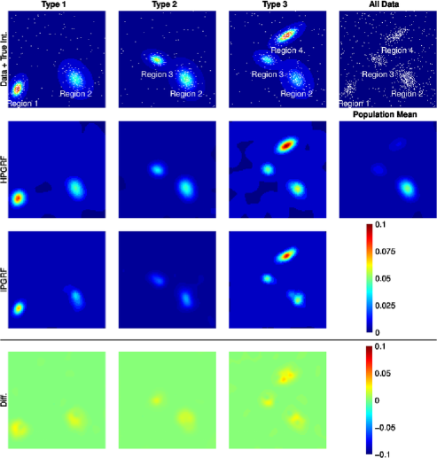
Figure 3: Image intensities in the simulation studies. Top row: True intensity functions with simulated data points from one realization. 2nd row: Estimated posterior mean intensity functions for the three types and for the population-level mean obtain from our HPGRF model for one simulation. 3rd row: Estimated posterior mean intensity functions obtained from the IPGRF model for one simulation. Bottom row: Difference image (HPGRF–IPGRF).

For comparison we fit a spatial point process for each emotion by extending the PGRF model to account for multiple independent realizations. We refer to this model as the independent PGRF (IPGRF) model. We simulate $K=1000$ data sets according to the model specifications in the previous section and fit each data set with the HPGRF model and the IPGRF models, respectively. Figure 3 shows the true intensity functions (top row) along with the estimated posterior mean intensity functions for one simulated data for both our HPGRF model (middle row) and the IPGRF model (bottom row). From this figure we see that both models do a good job, qualitatively, at reproducing the true intensity function. However, the HPGRF intensity appears to have regions of high intensity that are more elliptically shaped and closer to the truth.

Table 2: Simulation study results. Comparison of the IMSE and the IWMSE summary measures for our HPGRF model and the IPGRF model

	IMSE		IWMSE
Region	HPGRF (s.e.)	IPGRF (s.e.)	HPGRF (s.e.)	IPGRF (s.e.)
A	175.94 (22.42)	227.69 (25.57)	11.15 (2.68)	17.11 (2.60)
1	046.75 (10.24)	050.88 (11.83)	03.94 (1.07)	04.20 (1.04)
2	22.76 (6.76)	52.59 (9.53)	00.58 (0.19)	01.72 (0.34)
3	19.70 (4.55)	28.03 (5.86)	00.75 (0.24)	01.16 (0.26)
4	097.31 (16.95)	090.47 (19.40)	10.79 (2.38)	10.02 (2.38)

To quantify model performance, we compute the sub-type average integrated mean square error (IMSE) and integrated weighted mean square error (IWMSE) on region $A$. These quantities are defined, respectively, as

$$\operatorname{IMSE} = \frac{1}{JK}\sum_{j=1}^{J}\sum_{k=1}^{K}\int_{A}\bigl{[}\widetilde{\lambda}_{jk}(\mathrm{x})-\lambda_{j}(\mathrm{x})\bigr{]}^{2}\,d\mathrm{x},$$

$$\operatorname{IWMSE} = \frac{1}{JK}\sum_{j=1}^{J}\sum_{k=1}^{K}\int_{A}\bigl{[}\widetilde{\lambda}_{jk}(\mathrm{x})-\lambda_{j}(\mathrm{x})\bigr{]}^{2}\lambda_{j}(\mathrm{x})\,d\mathrm{x}.$$

Here $\widetilde{\lambda}_{jk}(\mathrm{x})$ is the type $j$ estimated posterior mean intensity function in the $k$th simulation and $\lambda_{j}(\mathrm{x})$ is the true intensity function. The IWMSE gives more weight to regions with a large true intensity. Table 2 summarizes the IMSE and the IWMSE in different regions. Over the entire region $A$, the IMSE and IWMSE are, respectively, 23% and 35% smaller under the HPGRF model than under the IPGRF model. In region 2 (within the true 0.95 probability ellipse), where all three types aggregate, the IMSE and IWMSE under the HPGRF model are 57% and 66% smaller than under the IPGRF model. In regions 1 and 4, where no inter-type aggregation occurs, both the HPGRF and IPGRF models give similar IMSE and IWMSE results (Table 2). Thus, when the different types of point patterns aggregate on a common region, the HPGRF model provides more accurate intensity estimates. When the types do not share any clustering on a region, the HPGRF has comparable performance with the IPGRF.

4 Application

The emotion meta-analysis data set consists of 164 publications designed to determine brain activation elicited by different emotions. Researchers collected both fMRI and PET data. Many articles report results from different statistical comparisons called “contrasts”, though we refer to each contrast as a “study”. We use a subset of the data, the 219 studies and 1393 foci for the five emotions sad, happy, anger, fear and disgust. In Figure 4 we display the locations of all foci from the five emotions.

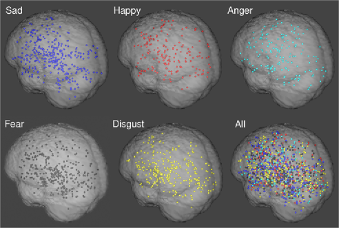
Figure 4: Data: The 1393 foci reported from 219 studies of five emotions.

Recall that we have four priors to specify: $\alpha(dx)$, $\beta$, $\tau$, and $\sigma_{j}^{2}$. We assume $\alpha(dx)$, the base measure of $G_{0}(dx)$, is Lebesgue measure. This implies that $\widetilde{\alpha}(dx)$ in Theorem 2 has a uniform distribution over $\mathcal{B}$ and the jump locations $\theta_{m}$ of the gamma random fields are uniformly distributed over $\mathcal{B}$, a priori. We assign the following prior distributions to the hyper-parameters: $\sigma^{-2}_{j}\sim U[0,10]$ and $\beta,\tau\sim\operatorname{Gamma}(2,2)$. We estimate the posterior on 100,000 iterations of simulation after a burn-in of 20,000, saving every 50th iteration. We truncate the infinite summation in the Lévy construction of the gamma random fields to $M=10\mbox{,}000$. This results in a posterior estimated truncation error of 0.01. We assess our model against both the IPGRF model and the BHICP model using a posterior predictive check in Section 4.1. We summarize results from a sensitivity analysis in Section 4.2 with details in the Web Supplementary Material, Section 3. We also summarize results from convergence diagnostics in Section 4.3.

We are interested in addressing the following questions. (1) Are there consistent activation regions (aggregation of foci) across studies of the same emotion? (2) Are there consistent activation regions across all emotion types? (3) Can we accurately predict the emotion elicited in a newly presented study? For questions (1) and (2) we focus on the amygdalae which are bilateral, almond-sized structures in the brain responsible for emotion processing [Adolphs (1999)], especially anger and fear.

(1) Are there consistent activation regions across studies of the same emotion? For each emotion type we estimate the expected posterior intensity function over the brain. We compare the intensity estimates between the HPGRF and the IPGRF models for axial slice $\mathrm{Z}=-18$ mm (see Figure 5). The intensity estimates are qualitatively similar, however, the HPGRF intensity estimate appears more spatially diffuse than the IPGRF intensity estimate. Furthermore, intensity estimates from the HPGRF model tend to be larger than those from the IPGRF model (Figure 5, 3rd row, where the difference between the HPGRF and IPGRF intensities are shown). These observations are a direct result of the fact that the jump locations of the gamma random fields are shared across emotions, and hence there is a borrowing of strength across the emotions.

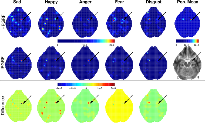
Figure 5: Top row: A single axial slice ($Z=-18$ mm) of the HPGRF posterior mean intensity estimates. (top row). Middle row: The corresponding IPGRF estimates. The arrows point to the right amygdala. All intensity functions have units of expected foci/mm³; the middle right image shows the corresponding brain anatomy. Bottom row: Difference image (HPGRF–IPGRF). Differences in this image can be clearly seen, especially the higher intensity estimate from the HPGRF model in the right amygdala due to borrowing of strength across the emotions.

All emotions show aggregation of foci, or consistent activation, in the amygdalae, although to varying degrees. This basic finding is consistent with previous meta-analytic summaries [Costafreda et al. (2008), Lindquist et al. (2012)]. The posterior intensity is larger in the left amygdala for fear and disgust, consistent with earlier findings of overall left-lateralization in the amygdala [Wager et al. (2003)] and relative specificity for fear and disgust [e.g., Costafreda et al. (2008), Wager et al. (2008), Lindquist et al. (2012), Yarkoni et al. (2010), Yue, Lindquist and Loh (2012)]. Sad and happy also show consistent activation in the left amygdala as well, whereas sad, happy, anger and fear also show strong right amygdala activation.

(2) Are there consistent activation regions across all emotion types? In line with the constructionist view of emotion processing, we are interested in determining whether different emotions activate the same areas of the brain, but perhaps, by varying degrees. This question can be reformulated as a question of whether there is inter-type (inter-emotion) aggregation of foci. To help answer this question we define a “population mean” intensity measure. Recall that $\Lambda_{j}(d\mathrm{y})$ is the intensity measure for each point process $\mathbf{Y}_{i,j}$. We define the “population mean” intensity measure by $\Lambda_{0}(d\mathrm{y})=\tau^{-1}\int_{\mathcal{B}}\widetilde{K}(d\mathrm{y},\mathrm{x})G_{0}(d\mathrm{x})$, where $\widetilde{K}(d\mathrm{y},\mathrm{x})=J^{-1}\sum_{j=1}^{J}K_{\sigma^{2}_{j}}(d\mathrm{y},\mathrm{x})$. Thus, $\Lambda_{0}(d\mathrm{y})$ is the average of the expected intensity measures of the different emotion types: $\Lambda_{0}(d\mathrm{y})=J^{-1}\sum_{j=1}^{J}E[\Lambda_{j}(d\mathrm{y})|G_{0},\sigma^{2}_{j},\tau]$.

The image in the first row, last column of Figure 5 shows a slice of the posterior mean of the “population level” intensity. This slice intersects the amygdalae with the arrow pointing to the right amygdala. There is relatively high intensity in the amygdalae, confirming the importance of these brain structures in the processing of emotions.

To measure the extent to which different emotions share common activation regions we estimate the posterior correlations between the different emotions in the amygdalae based on Theorem 1. The average posterior correlations between the different emotions in the left amygdala range from 0.69 to 0.71 and for the right amygdala from 0.74 to 0.75. Thus, the data suggest that in each amygdala the activation pattern among the five emotions are highly correlated. This lends credence to the constructionist theory which attests that all emotions elicit response in similar regions of the brain, but perhaps to varying degrees, at least in the amygdalae.

(3) Can we accurately predict the emotion elicited in a newly presented study? As described in the Introduction, “reverse inference” is used to infer the most likely class of task to give rise to a particular study. Such predictive inferences are straightforward with our HPGRF model. Over the domain of five emotion subtypes, we can use a single study’s foci to make predictions about the emotion type of that study.

We compare our predictive method to previous work that combines the MKDA and a naïve Bayesian classifier (NBC) [Yarkoni et al. (2011)]. For each study, this method creates binary activation maps using the MKDA, with a value of 1 (activated) assigned to each voxel in the brain if it is within a certain distance (a spherical kernel size) of a reported focus, and 0 (nonactivated) otherwise. These binary activation maps are in turn treated as feature variables in the NBC. The study type, that is, the designed psychological state, determines the class membership. Specifically, for each type, an activation probability map is constructed by a weighted average of the binary maps. Using the activation probability maps, the predictive probability of the study type given activation from a new study is then computed based on Bayes’ theorem under an assumption of independent voxels [see Yarkoni et al. (2011) for details]. This method is very computationally efficient and can handle extremely large sets of voxels without difficulty. However, there are several potential drawbacks of this method. First, NBC ignores the spatial dependence in the activation maps, leading to biased predictive probabilities of the class membership. Second, MKDA requires a fixed tuning parameter—the kernel radius—that might affect classification performance: currently MKDA simply fixes the kernel radius to some constant based on experience rather than estimating it from data. Third, it only focuses on the difference in the spatial distributions of foci between groups while neglecting the absolute rates of foci, which may be important for classification.

Our model has at least three advantages compared with the MKDA based NBC. First, in the CBMA data, the number of foci and their locations are random. Our HPGRF model explicitly models both the random number and random locations of foci, as well as the spatial dependence between foci. These features of the data are not modeled by the MKDA based NBC. Second, our model is a more accurate representation of the true data generating process, relative to how MKDA maps points to a voxel-wise image with a spherical kernel. Third, our Bayesian model captures more sources of variation and appropriately conveys the uncertainty in the computation of the predictive probabilities that determines the classification.

We use Bayes’ theorem to perform prediction using a leave-on-out cross validation (LOOCV) approach. Details are given in the Web Supplementary Material, Section 4. We assume equal prior probability for each emotion, and fit our Bayesian spatial point process classifier using the HPGRF model. As a comparison, we also fit the classifier using the IPGRF model. Table 3 shows the LOOCV classifications rates based on our HPGRF/IPGRF models as well as those based on the MKDA using the NBC. Our spatial classifier correctly classifies 188 of the 219 studies, for overall correct classification rate of $0.86\pm 0.024$ (mean $\pm$ standard error), far above random chance of 0.20. A simple average of correct classification rates over emotions provides an average correct classification rate of $0.85\pm 0.024$. The IPGRF based classifier provides lower classification accuracy with the overall correct classification rate of $0.75\pm 0.029$ and average correct classification rate of $0.75\pm 0.029$. The MKDA based NBC (kernel radius is 10 mm) correctly classifies 99 studies with an overall correct classification rate of $0.45\pm 0.034$ and an average correct classification rate of $0.36\pm 0.032$. Changing the MKDA kernel radius to 5 mm, 15 mm and 20 mm did not improve the method’s accuracy.

Table 3: Confusion matrices of the LOOCV classification. For the naïve Bayesian classifier the overall correct classification rate is $0.45\pm 0.034$ (mean $\pm$ s.e.) and the average correct classification rate is $0.36\pm 0.032$. For the independent Poisson/gamma random field model the overall correct rate and average rate are both $0.75\pm 0.029$. For the hierarchical Poisson/gamma random field model the overall correct classification rate is $0.86\pm 0.024$ and the average rate is $0.85\pm 0.024$. The largest standard error, based on the multinomial distribution, for any of the methods for any emotion is 0.10

		Confusion matrices
	Truth	Sad	Happy	Anger	Fear	Disgust
MKDA-NBC	sad	0.38	0.11	0.07	0.40	0.04
	happy	0.11	0.25	0.03	0.56	0.06
	anger	0.12	0.23	0.00	0.50	0.15
	fear	0.06	0.06	0.01	0.81	0.06
	disgust	0.09	0.16	0.05	0.32	0.39
IPGRF	sad	0.78	0.09	0.04	0.07	0.02
	happy	0.00	0.81	0.03	0.17	0.00
	anger	0.00	0.04	0.69	0.27	0.00
	fear	0.03	0.13	0.06	0.72	0.06
	disgust	0.02	0.09	0.02	0.09	0.77
HPGRF	sad	0.91	0.04	0.00	0.04	0.00
	happy	0.00	0.83	0.08	0.08	0.00
	anger	0.00	0.12	0.77	0.12	0.00
	fear	0.01	0.07	0.04	0.85	0.01
	disgust	0.02	0.05	0.02	0.02	0.89

Thus, our model based classifier does a good job at predicting the emotion actually studied. The emotions anger and happy, when they are misclassified, tend to be misclassified as fear. This finding contradicts the simple assumption that similarity in our subjective experience implies similarity in the brain processes that underlie emotion. That assumption has driven psychologically based theories of affect, such as the valence-arousal model Russell and Barrett (1999), that organize emotion based on direct experience. By contrast, our method provides some early steps toward establishing taxonomies of emotion based on similarity in brain activity patterns. Such taxonomies may be based on properties that are identifiable at a psychological level–for example, fear, anger, and happy all involve an aroused, activated state, whereas disgust and sadness may not to the same degree–but they need not respect our psychological distinctions. These taxonomies are also relative to the level of analysis and spatial resolution one considers: For example, neurons that encode negative and positive information are intermixed in the amygdalae [Paton et al. (2006)], and thus may elicit confusability between these types at the coarse meta-analytic level of resolution. In short, the entire confusion matrix provides information on the nature of emotion processing in the brain.

4.1 Model assessment

As a measure of model fit, we conduct a posterior predictive model check using the $L$ function, a summary statistic for second order properties of a point process [Baddeley, Møller and Waagepetersen (2000), Illian, Møller and Waagepetersen (2009), Kang et al. (2011)]. The $L$ function can indicate aggregation or clustering for a point process. For our model, $L(r;\cdot)=\{3K(r;\cdot)/4\pi\}^{1/3}$, where

$$K(r;\mathbf{Y}_{i,j},\cdot)=\frac{1}{|\mathcal{B}|}\sum_{y_{1},y_{2}\in\mathbf{Y}_{i,j}}\frac{\mathbf{1}[\|y_{1}-y_{2}\|\leq r]}{\lambda_{1c}(y_{1};\cdot)\lambda_{1c}(y_{2};\cdot)}.$$

Consider the posterior predictive distribution of the differences $\Delta_{i,j}(r)=L(r;\mathbf{Y}_{i,j},\cdot)-L(r;\mathbf{Y}^{*}_{i,j},\cdot)$, where $\mathbf{Y}^{*}_{i,j}$ is a simulated sample from the posterior predictive distribution for study $i$ and type $j$. For a range of distances $r$, if zero is an extreme value in the posterior predictive distribution of $\Delta_{i,j}(r)$, then we question the fit of the model [Illian, Møller and Waagepetersen (2009), Kang et al. (2011)]. For $r>0$, we estimate the 95% posterior credible curves (as a function of $r$) of $\Delta_{i,j}(r)$, for each the 219 studies. We consider zero an extreme value at a distance $r$ if it lies outside of the 95% posterior interval. We regard the model a good fit for a study if zero is an extreme value in less than 10% of its range. For our HPGRF model, the model is a good fit for all 219 studies (100%). For the IPGRF model, the model is a good fit for only 138 studies (63%). Finally, for the parametric BHICP model, the model is a good fit for only 142 studies (65%). Thus, overall, our HPGRF model provides a substantially better fit to the data based on this posterior predictive assessment.

4.2 Sensitivity analysis

We conduct a sensitivity analysis of the posterior intensity function as a function of prior parameter distributions (for $\sigma_{j}^{-2}$, $\beta$, $\tau$ and $M$). We simulate the posterior using nine different scenarios as shown in Table A in the Web Supplementary Material [Kang et al. (2014)], where Figure C presents one axial slice ($Z=-18$ mm) of the full 3D posterior mean intensity maps for different scenarios. They looks qualitatively similar. Also, Table B in the Web Supplementary Material [Kang et al. (2014)] shows, for each emotion and for the overall population, the minimum, median and maximum for the expected posterior intensity function. These results show that the posterior is not sensitive to the prior distributions over these nine scenarios.

4.3 Convergence diagnostics and reproducibility

We also monitor convergence. We would like to monitor convergence of the posterior intensity functions at each voxel. However, this is impractical due to the extremely large number of voxels. Instead, we run the model three separate times, with different random number generation seeds and from over-dispersed starting values. From these three runs we determine the location of the maximum difference in the posterior intensity functions for each of the five emotions. We also select ten other locations for which we monitor convergence. Some of these locations are where the posterior intensity is larger and others where it is small. These locations are chosen throughout the brain. We also compute and save the integrated intensity functions (the posterior expected number of foci for each study in each emotion type). We then rerun the posterior simulation three more times, saving the posterior draws of the intensity functions and using the Gelman–Rubin convergence diagnostic for multiple chains [Gelman and Rubin (1992)]. We use a burnin of 20,000 and run the chain for another 25,000 iterations and save values at every 25th iteration for a total of 1000 saved draws from the posterior (note that this is a smaller burnin period and a short overall simulation than for the data analysis). The largest scale reduction factor is 1.02 and the multivariate scale reduction factor is 1.09 [Brooks and Gelman (1998)]. A multivariate scale reduction factor near 1 indicates convergence. From these results we are confident that our chain has reached stationarity and that posterior estimates of intensity functions can be reliably reproduced.

5 Discussion

In this article, we propose a Bayesian nonparametric spatial point process model, the HPGRF model, by generalizing the PGRF model introduced by Wolpert and Ickstadt (1998a) to hierarchical spatial point process models. Our HPGRF model is appropriate for multi-type spatial point pattern data when there is aggregation between and within types. It accounts for positive dependence in the point patterns both within and between types. That is, it allows and models aggregation between points within types and between points across types. Our model also allows for multiple, independent, realizations of the spatial point process within each type—as is demonstrated with the neuroimaging meta-analysis example in Section 4. We note here, that if there is repulsion between types, such as when there is competition between species for resources in ecological data, our model is not appropriate.

In our example analyses we provide “population mean” intensity estimates to identify common regions that share clustering, or aggregation, providing better interpretation of data. Results from the emotion meta-analysis also lend support to the constructionist view of emotions. The LOOCV results demonstrate that, at least for prediction purposes, our model is more appropriate than the IPGRF model and greatly outperforms a simple naïve Bayes classifier. This performance difference is evidence that the point process approach captures important spatial and stochastic features of CBMA data. Such classification results are also a first step in allowing users of fMRI to make “reverse inferences” [Poldrack (2011)].

The simulation studies shows that the HPGRF model improves intensity estimate accuracy over the IPGRF model when aggregation is present across types and does not suffer a loss of accuracy when the point patterns arising from the different types are independent of one another. Posterior predictive checks also indicate that our model fits the data better than both the IPGRF and the BHICP models. Sensitivity analyses and convergence diagnostics demonstrate that our model is robust to prior specification and that posterior estimation of the intensity function is reproducible.

Like the PGRF model, the HPGRF model can accommodate non stationary processes by include spatially varying covariates. For example with a single spatially varying covariate, $\mathbf{Z}(\mathrm{y})$ say, using a semi-parametric regression approach, the random intensity measure for each type $j$ can be modeled as $\tilde{\Lambda}_{j}(d\mathrm{y};\mathbf{Z})=\Lambda_{j}(d\mathrm{y})\exp\{\mathbf{Z}(\mathrm{y}){\bolds\beta_{j}}\}$. We can also assign an hierarchical prior on $\bolds\beta_{j}$ such that the posterior estimates of $\bolds\beta_{j}$ borrow information across different types. $\Lambda_{j}(d\mathrm{y})$ is interpreted as the baseline intensity measure and $\bolds\beta_{j}$ represents the spatial covariate effect for type $j$.

There are several directions one can take to extend our model further. First, the HPGRF model can be extended to more than two levels of hierarchy to deal with more complex spatial point patterns. The depth of the hierarchy would depend on the needs of the data analysis. For instance, in the functional neuroimaging meta-analyses of emotion, there are positive emotions (e.g., happy and affective) and negative emotions (e.g., fear and disgust). One problem of interest is to identify the common consistent activation regions for positive emotions, negative emotions, and all emotions. This motivates the needs for a third level in hierarchy: the first level models each type of emotion; the second level models positive/negative emotions and the third level models the entire population of emotions. Another interesting extension is to allow the HPGRF model to accommodate multiple dependent realizations of multi-type spatial point processes. A practical use for such a model is the analysis of spatio-temporal point pattern data, even for a single type.

Computationally, the Lévy construction relies on the truncation of an infinite sum. The number of points, $M$, in the gamma random field typically must be very large to achieve a reasonable level of accuracy for the intensity estimates, thus the computation cost can be high. The analysis present in Section 4 takes approximately 20 hours on a MAC Pro with 8 Gb of memory and a 3.0 GHz Intel processor.

There is potential to speed up the computation. One possible solution is to approximate the gamma random field using a marked point process according to the Lévy construction, where a point represents the location of a jump and the mark is the height of the jump. Then we can utilize the spatial birth–death process to simulate a gamma random field with a random number of jumps. Currently, we are evaluating the possibility of leveraging the relationship between the gamma process and the Dirichlet process [Ferguson (1973)] and modifying one of the many algorithms developed for Dirichlet process models [see, Walker (2007), e.g., which appears quite promising] for our HPGRF model.

Code is available by contacting the first author.

References

- Adolphs (1999) {barticle}[auto:STB—2014/08/04—07:23:14] \bauthor\bsnmAdolphs, \bfnmR.\binitsR. (\byear1999). \btitleThe human amygdala and emotion. \bjournalNeuroscientist \bvolume5 \bpages125–137. \bptokimsref\endbibitem
- Baddeley, Møller and Waagepetersen (2000) {barticle}[mr] \bauthor\bsnmBaddeley, \bfnmA. J.\binitsA. J., \bauthor\bsnmMøller, \bfnmJ.\binitsJ. and \bauthor\bsnmWaagepetersen, \bfnmR.\binitsR. (\byear2000). \btitleNon- and semi-parametric estimation of interaction in inhomogeneous point patterns. \bjournalStat. Neerl. \bvolume54 \bpages329–350. \biddoi=10.1111/1467-9574.00144, issn=0039-0402, mr=1804002 \bptokimsref\endbibitem
- Best, Ickstadt and Wolpert (2000) {barticle}[mr] \bauthor\bsnmBest, \bfnmNicola G.\binitsN. G., \bauthor\bsnmIckstadt, \bfnmKatja\binitsK. and \bauthor\bsnmWolpert, \bfnmRobert L.\binitsR. L. (\byear2000). \btitleSpatial Poisson regression for health and exposure data measured at disparate resolutions. \bjournalJ. Amer. Statist. Assoc. \bvolume95 \bpages1076–1088. \biddoi=10.2307/2669744, issn=0162-1459, mr=1821716 \bptokimsref\endbibitem
- Best et al. (2002) {bincollection}[mr] \bauthor\bsnmBest, \bfnmNicola G.\binitsN. G., \bauthor\bsnmIckstadt, \bfnmKatja\binitsK., \bauthor\bsnmWolpert, \bfnmRobert L.\binitsR. L., \bauthor\bsnmCockings, \bfnmSamantha\binitsS., \bauthor\bsnmElliott, \bfnmPaul\binitsP., \bauthor\bsnmBennett, \bfnmJames\binitsJ., \bauthor\bsnmBottle, \bfnmAlex\binitsA. and \bauthor\bsnmReed, \bfnmSean\binitsS. (\byear2002). \btitleModeling the impact of traffic-related air pollution on childhood respiratory illness. In \bbooktitleCase Studies in Bayesian Statistics, Vol. V (Pittsburgh, PA, 1999) (\beditor\binitsC.\bfnmC. \bsnmGatsonis, \beditor\binitsR.\bfnmR. \bsnmKass, \beditor\binitsB.\bfnmB. \bsnmCarlin, \beditor\binitsA.\bfnmA. \bsnmCarriquiry, \beditor\binitsA.\bfnmA. \bsnmGelman, \beditor\binitsI.\bfnmI. \bsnmVerdinelli and \beditor\binitsM.\bfnmM. \bsnmWest, eds.). \bseriesLecture Notes in Statist. \bvolume162 \bpages183–259. \bpublisherSpringer, \blocationNew York. \biddoi=10.1007/978-1-4613-0035-9_3, mr=1931868 \bptnotecheck related \bptokimsref\endbibitem
- Bondesson (1982) {barticle}[mr] \bauthor\bsnmBondesson, \bfnmLennart\binitsL. (\byear1982). \btitleOn simulation from infinitely divisible distributions. \bjournalAdv. in Appl. Probab. \bvolume14 \bpages855–869. \biddoi=10.2307/1427027, issn=0001-8678, mr=0677560 \bptokimsref\endbibitem
- Brooks and Gelman (1998) {barticle}[mr] \bauthor\bsnmBrooks, \bfnmStephen P.\binitsS. P. and \bauthor\bsnmGelman, \bfnmAndrew\binitsA. (\byear1998). \btitleGeneral methods for monitoring convergence of iterative simulations. \bjournalJ. Comput. Graph. Statist. \bvolume7 \bpages434–455. \biddoi=10.2307/1390675, issn=1061-8600, mr=1665662 \bptokimsref\endbibitem
- Costafreda et al. (2008) {barticle}[auto:STB—2014/08/04—07:23:14] \bauthor\bsnmCostafreda, \bfnmS. G.\binitsS. G., \bauthor\bsnmBrammer, \bfnmM. J.\binitsM. J., \bauthor\bsnmDavid, \bfnmA. S.\binitsA. S. and \bauthor\bsnmFu, \bfnmC. H. Y.\binitsC. H. Y. (\byear2008). \btitlePredictors of amygdala activation during the processing of emotional stimuli: A meta-analysis of 385 PET and fMRI studies. \bjournalBrain Research Reviews \bvolume58 \bpages57–70. \bptokimsref\endbibitem
- Cox (1955) {barticle}[mr] \bauthor\bsnmCox, \bfnmD. R.\binitsD. R. (\byear1955). \btitleSome statistical methods connected with series of events. \bjournalJ. R. Stat. Soc. Ser. B Stat. Methodol. \bvolume17 \bpages129–157; discussion, 157–164. \bidissn=0035-9246, mr=0092301 \bptnotecheck related \bptokimsref\endbibitem
- Damien, Laud and Smith (1995) {barticle}[mr] \bauthor\bsnmDamien, \bfnmPaul\binitsP., \bauthor\bsnmLaud, \bfnmPurushottam W.\binitsP. W. and \bauthor\bsnmSmith, \bfnmAdrian F. M.\binitsA. F. M. (\byear1995). \btitleApproximate random variate generation from infinitely divisible distributions with applications to Bayesian inference. \bjournalJ. R. Stat. Soc. Ser. B Stat. Methodol. \bvolume57 \bpages547–563. \bidissn=0035-9246, mr=1341323 \bptokimsref\endbibitem
- Eickhoff et al. (2009) {barticle}[pbm] \bauthor\bsnmEickhoff, \bfnmSimon B.\binitsS. B., \bauthor\bsnmLaird, \bfnmAngela R.\binitsA. R., \bauthor\bsnmGrefkes, \bfnmChristian\binitsC., \bauthor\bsnmWang, \bfnmLing E.\binitsL. E., \bauthor\bsnmZilles, \bfnmKarl\binitsK. and \bauthor\bsnmFox, \bfnmPeter T.\binitsP. T. (\byear2009). \btitleCoordinate-based activation likelihood estimation meta-analysis of neuroimaging data: A random-effects approach based on empirical estimates of spatial uncertainty. \bjournalHum. Brain Mapp. \bvolume30 \bpages2907–2926. \biddoi=10.1002/hbm.20718, issn=1097-0193, mid=NIHMS95486, pmcid=2872071, pmid=19172646 \bptokimsref\endbibitem
- Ferguson (1973) {barticle}[mr] \bauthor\bsnmFerguson, \bfnmThomas S.\binitsT. S. (\byear1973). \btitleA Bayesian analysis of some nonparametric problems. \bjournalAnn. Statist. \bvolume1 \bpages209–230. \bidissn=0090-5364, mr=0350949 \bptokimsref\endbibitem
- Fox et al. (1997) {barticle}[pbm] \bauthor\bsnmFox, \bfnmP. T.\binitsP. T., \bauthor\bsnmLancaster, \bfnmJ. L.\binitsJ. L., \bauthor\bsnmParsons, \bfnmL. M.\binitsL. M., \bauthor\bsnmXiong, \bfnmJ. H.\binitsJ. H. and \bauthor\bsnmZamarripa, \bfnmF.\binitsF. (\byear1997). \btitleFunctional volumes modeling: Theory and preliminary assessment. \bjournalHum. Brain Mapp. \bvolume5 \bpages306–311. \biddoi=10.1002/(SICI)1097-0193(1997)5:4¡306::AID-HBM17¿3.0.CO;2-B, issn=1065-9471, pmid=20408233 \bptokimsref\endbibitem
- Gelman and Rubin (1992) {barticle}[auto:STB—2014/08/04—07:23:14] \bauthor\bsnmGelman, \bfnmA.\binitsA. and \bauthor\bsnmRubin, \bfnmD. B.\binitsD. B. (\byear1992). \btitleInference from iterative simulation using multiple sequences. \bjournalStatist. Sci. \bvolume7 \bpages457–472. \bptokimsref\endbibitem
- Iacoboni et al. (2007) {bmisc}[auto:STB—2014/08/04—07:23:14] \bauthor\bsnmIacoboni, \bfnmM.\binitsM., \bauthor\bsnmFreedman, \bfnmJ.\binitsJ., \bauthor\bsnmKaplan, \bfnmJ.\binitsJ., \bauthor\bsnmJamieson, \bfnmK. H.\binitsK. H., \bauthor\bsnmFreedman, \bfnmT.\binitsT., \bauthor\bsnmKnapp, \bfnmB.\binitsB. and \bauthor\bsnmFitzgerald, \bfnmK.\binitsK. (\byear2007). \bhowpublishedThis is your brain on politics. The New York Times. \bptokimsref\endbibitem
- Ickstadt and Wolpert (1999) {bincollection}[mr] \bauthor\bsnmIckstadt, \bfnmKatja\binitsK. and \bauthor\bsnmWolpert, \bfnmRobert L.\binitsR. L. (\byear1999). \btitleSpatial regression for marked point processes. In \bbooktitleBayesian Statistics, 6 (Alcoceber, 1998) (\beditor\binitsJ.\bfnmJ. \bsnmBernardo, \beditor\binitsJ.\bfnmJ. \bsnmBerger, \beditor\binitsA.\bfnmA. \bsnmDawid and \beditor\binitsA.\bfnmA. \bsnmSmith, eds.) \bpages323–341. \bpublisherOxford Univ. Press, \blocationNew York. \bidmr=1723503 \bptnotecheck related \bptokimsref\endbibitem
- Illian, Møller and Waagepetersen (2009) {barticle}[mr] \bauthor\bsnmIllian, \bfnmJanine B.\binitsJ. B., \bauthor\bsnmMøller, \bfnmJesper\binitsJ. and \bauthor\bsnmWaagepetersen, \bfnmRasmus P.\binitsR. P. (\byear2009). \btitleHierarchical spatial point process analysis for a plant community with high biodiversity. \bjournalEnviron. Ecol. Stat. \bvolume16 \bpages389–405. \biddoi=10.1007/s10651-007-0070-8, issn=1352-8505, mr=2749847 \bptokimsref\endbibitem
- Illian et al. (2008) {bbook}[mr] \bauthor\bsnmIllian, \bfnmJanine\binitsJ., \bauthor\bsnmPenttinen, \bfnmAntti\binitsA., \bauthor\bsnmStoyan, \bfnmHelga\binitsH. and \bauthor\bsnmStoyan, \bfnmDietrich\binitsD. (\byear2008). \btitleStatistical Analysis and Modelling of Spatial Point Patterns. \bpublisherWiley, \blocationChichester. \bidmr=2384630 \bptokimsref\endbibitem
- Kang et al. (2014) {bmisc}[author] \bauthor\bsnmKang, \binitsJ., \bauthor\bsnmNichols, \binitsT. E., \bauthor\bsnmWager, \binitsT. D. and \bauthor\bsnmJohnson, \binitsT. D. (\byear2014). \bhowpublishedSupplement to “A Bayesian hierarchical spatial point process model for multi-type neuroimaging meta-analysis.” DOI:\doiurl10.1214/14-AOAS757SUPP. \bptokimsref \endbibitem
- Kang et al. (2011) {barticle}[mr] \bauthor\bsnmKang, \bfnmJian\binitsJ., \bauthor\bsnmJohnson, \bfnmTimothy D.\binitsT. D., \bauthor\bsnmNichols, \bfnmThomas E.\binitsT. E. and \bauthor\bsnmWager, \bfnmTor D.\binitsT. D. (\byear2011). \btitleMeta analysis of functional neuroimaging data via Bayesian spatial point processes. \bjournalJ. Amer. Statist. Assoc. \bvolume106 \bpages124–134. \biddoi=10.1198/jasa.2011.ap09735, issn=0162-1459, mr=2816707 \bptokimsref\endbibitem
- Kober et al. (2008) {barticle}[auto:STB—2014/08/04—07:23:14] \bauthor\bsnmKober, \bfnmH.\binitsH., \bauthor\bsnmBarrett, \bfnmL. F.\binitsL. F., \bauthor\bsnmJoseph, \bfnmJ.\binitsJ., \bauthor\bsnmBliss-Moreau, \bfnmE.\binitsE., \bauthor\bsnmLindquist, \bfnmK.\binitsK. and \bauthor\bsnmWager, \bfnmT. D.\binitsT. D. (\byear2008). \btitleFunctional grouping and cortical–subcortical interactions in emotion: A meta-analysis of neuroimaging studies. \bjournalNeuroImage \bvolume42 \bpages998–1031. \bptokimsref\endbibitem
- Lindquist et al. (2012) {barticle}[pbm] \bauthor\bsnmLindquist, \bfnmKristen A.\binitsK. A., \bauthor\bsnmWager, \bfnmTor D.\binitsT. D., \bauthor\bsnmKober, \bfnmHedy\binitsH., \bauthor\bsnmBliss-Moreau, \bfnmEliza\binitsE. and \bauthor\bsnmBarrett, \bfnmLisa Feldman\binitsL. F. (\byear2012). \btitleThe brain basis of emotion: A meta-analytic review. \bjournalBehav. Brain Sci. \bvolume35 \bpages121–143. \biddoi=10.1017/S0140525X11000446, issn=1469-1825, pii=S0140525X11000446, pmid=22617651 \bptokimsref\endbibitem
- Møller, Syversveen and Waagepetersen (1998) {barticle}[mr] \bauthor\bsnmMøller, \bfnmJesper\binitsJ., \bauthor\bsnmSyversveen, \bfnmAnne Randi\binitsA. R. and \bauthor\bsnmWaagepetersen, \bfnmRasmus Plenge\binitsR. P. (\byear1998). \btitleLog Gaussian Cox processes. \bjournalScand. J. Stat. \bvolume25 \bpages451–482. \biddoi=10.1111/1467-9469.00115, issn=0303-6898, mr=1650019 \bptokimsref\endbibitem
- Møller and Waagepetersen (2004) {bbook}[mr] \bauthor\bsnmMøller, \bfnmJesper\binitsJ. and \bauthor\bsnmWaagepetersen, \bfnmRasmus Plenge\binitsR. P. (\byear2004). \btitleStatistical Inference and Simulation for Spatial Point Processes. \bseriesMonographs on Statistics and Applied Probability \bvolume100. \bpublisherChapman & Hall/CRC, \blocationBoca Raton, FL. \bidmr=2004226 \bptokimsref\endbibitem
- Møller and Waagepetersen (2007) {barticle}[mr] \bauthor\bsnmMøller, \bfnmJesper\binitsJ. and \bauthor\bsnmWaagepetersen, \bfnmRasmus P.\binitsR. P. (\byear2007). \btitleModern statistics for spatial point processes. \bjournalScand. J. Stat. \bvolume34 \bpages643–684. \biddoi=10.1111/j.1467-9469.2007.00569.x, issn=0303-6898, mr=2392447 \bptnotecheck related \bptokimsref\endbibitem
- Nielsen and Hansen (2002) {barticle}[pbm] \bauthor\bsnmNielsen, \bfnmFinn Arup\binitsF. A. and \bauthor\bsnmHansen, \bfnmLars Kai\binitsL. K. (\byear2002). \btitleModeling of activation data in the BrainMap database: Detection of outliers. \bjournalHum. Brain Mapp. \bvolume15 \bpages146–156. \bidissn=1065-9471, pii=10.1002/hbm.10012, pmid=11835605 \bptokimsref\endbibitem
- Niemi and Fernández (2010) {barticle}[mr] \bauthor\bsnmNiemi, \bfnmAki\binitsA. and \bauthor\bsnmFernández, \bfnmCarmen\binitsC. (\byear2010). \btitleBayesian spatial point process modeling of line transect data. \bjournalJ. Agric. Biol. Environ. Stat. \bvolume15 \bpages327–345. \biddoi=10.1007/s13253-010-0024-8, issn=1085-7117, mr=2787262 \bptokimsref\endbibitem
- Paton et al. (2006) {barticle}[auto:STB—2014/08/04—07:23:14] \bauthor\bsnmPaton, \bfnmJ. J.\binitsJ. J., \bauthor\bsnmBelova, \bfnmM. A.\binitsM. A., \bauthor\bsnmMorrison, \bfnmS. E.\binitsS. E. and \bauthor\bsnmSalzman, \bfnmC. D.\binitsC. D. (\byear2006). \btitleThe primate amygdala represents the positive and negative value of visual stimuli during learning. \bjournalNature \bvolume439 \bpages865–870. \bptokimsref\endbibitem
- Poldrack (2011) {barticle}[auto:STB—2014/08/04—07:23:14] \bauthor\bsnmPoldrack, \bfnmR. A.\binitsR. A. (\byear2011). \btitleInferring mental states from neuroimaging data: From reverse inference to large-scale decoding. \bjournalNeuron \bvolume72 \bpages692–697. \bptokimsref\endbibitem
- Radua and Mataix-Cols (2009) {barticle}[pbm] \bauthor\bsnmRadua, \bfnmJoaquim\binitsJ. and \bauthor\bsnmMataix-Cols, \bfnmDavid\binitsD. (\byear2009). \btitleVoxel-wise meta-analysis of grey matter changes in obsessive-compulsive disorder. \bjournalBr. J. Psychiatry \bvolume195 \bpages393–402. \biddoi=10.1192/bjp.bp.108.055046, issn=1472-1465, pii=195/5/393, pmid=19880927 \bptokimsref\endbibitem
- Russell and Barrett (1999) {barticle}[pbm] \bauthor\bsnmRussell, \bfnmJ. A.\binitsJ. A. and \bauthor\bsnmBarrett, \bfnmL. F.\binitsL. F. (\byear1999). \btitleCore affect, prototypical emotional episodes, and other things called emotion: Dissecting the elephant. \bjournalJ. Pers. Soc. Psychol. \bvolume76 \bpages805–819. \bidissn=0022-3514, pmid=10353204 \bptokimsref\endbibitem
- Stoyan and Penttinen (2000) {barticle}[mr] \bauthor\bsnmStoyan, \bfnmDietrich\binitsD. and \bauthor\bsnmPenttinen, \bfnmAntti\binitsA. (\byear2000). \btitleRecent applications of point process methods in forestry statistics. \bjournalStatist. Sci. \bvolume15 \bpages61–78. \biddoi=10.1214/ss/1009212674, issn=0883-4237, mr=1842237 \bptokimsref\endbibitem
- Teh et al. (2006) {barticle}[mr] \bauthor\bsnmTeh, \bfnmYee Whye\binitsY. W., \bauthor\bsnmJordan, \bfnmMichael I.\binitsM. I., \bauthor\bsnmBeal, \bfnmMatthew J.\binitsM. J. and \bauthor\bsnmBlei, \bfnmDavid M.\binitsD. M. (\byear2006). \btitleHierarchical Dirichlet processes. \bjournalJ. Amer. Statist. Assoc. \bvolume101 \bpages1566–1581. \biddoi=10.1198/016214506000000302, issn=0162-1459, mr=2279480 \bptokimsref\endbibitem
- Turkeltaub et al. (2002) {barticle}[pbm] \bauthor\bsnmTurkeltaub, \bfnmPeter E.\binitsP. E., \bauthor\bsnmEden, \bfnmGuinevere F.\binitsG. F., \bauthor\bsnmJones, \bfnmKaren M.\binitsK. M. and \bauthor\bsnmZeffiro, \bfnmThomas A.\binitsT. A. (\byear2002). \btitleMeta-analysis of the functional neuroanatomy of single-word reading: Method and validation. \bjournalNeuroimage \bvolume16 \bpages765–780. \bidissn=1053-8119, pii=S1053811902911316, pmid=12169260 \bptokimsref\endbibitem
- van Lieshout and Baddeley (2002) {bincollection}[mr] \bauthor\bparticlevan \bsnmLieshout, \bfnmM. N. M.\binitsM. N. M. and \bauthor\bsnmBaddeley, \bfnmA. J.\binitsA. J. (\byear2002). \btitleExtrapolating and interpolating spatial patterns. In \bbooktitleSpatial Cluster Modelling (\beditor\binitsA. B.\bfnmA. B. \bsnmLawson and \beditor\binitsD. G. T.\bfnmD. G. T. \bsnmDenison, eds.) \bpages61–86. \bpublisherChapman & Hall/CRC, \blocationBoca Raton, FL. \bidmr=2015031 \bptokimsref\endbibitem
- Wager, Jonides and Reading (2004) {barticle}[pbm] \bauthor\bsnmWager, \bfnmTor D.\binitsT. D., \bauthor\bsnmJonides, \bfnmJohn\binitsJ. and \bauthor\bsnmReading, \bfnmSusan\binitsS. (\byear2004). \btitleNeuroimaging studies of shifting attention: A meta-analysis. \bjournalNeuroimage \bvolume22 \bpages1679–1693. \biddoi=10.1016/j.neuroimage.2004.03.052, issn=1053-8119, pii=S105381190400223X, pmid=15275924 \bptokimsref\endbibitem
- Wager et al. (2003) {barticle}[auto:STB—2014/08/04—07:23:14] \bauthor\bsnmWager, \bfnmT. D.\binitsT. D., \bauthor\bsnmPhan, \bfnmK.\binitsK., \bauthor\bsnmLiberzon, \bfnmI.\binitsI. and \bauthor\bsnmTaylor, \bfnmS. F.\binitsS. F. (\byear2003). \btitleValence, gender, and lateralization of functional brain anatomy in emotion: A meta-analysis of findings from neuroimaging. \bjournalNeuroImage \bvolume19 \bpages513–531. \bptokimsref\endbibitem
- Wager et al. (2008) {bincollection}[auto:STB—2014/08/04—07:23:14] \bauthor\bsnmWager, \bfnmT. D.\binitsT. D., \bauthor\bsnmBarrett, \bfnmL. F.\binitsL. F., \bauthor\bsnmBliss-moreau, \bfnmE.\binitsE., \bauthor\bsnmLindquist, \bfnmK. A.\binitsK. A., \bauthor\bsnmDuncan, \bfnmS.\binitsS., \bauthor\bsnmKober, \bfnmH.\binitsH., \bauthor\bsnmJoseph, \bfnmJ.\binitsJ., \bauthor\bsnmDavidson, \bfnmM.\binitsM. and \bauthor\bsnmMize, \bfnmJ.\binitsJ. (\byear2008). \btitleThe neuroimaging of emotion. In \bbooktitleHandbook of Emotions, Chapter 15 (\beditor\binitsM.\bfnmM. \bsnmLewis, \beditor\binitsJ. M.\bfnmJ. M. \bsnmHaviland-Jones and \beditor\binitsL. F.\bfnmL. F. \bsnmBarrett, eds.) \bpages848. \bpublisherGuilford, \blocationNew York. \bptokimsref\endbibitem
- Walker (2007) {barticle}[mr] \bauthor\bsnmWalker, \bfnmStephen G.\binitsS. G. (\byear2007). \btitleSampling the Dirichlet mixture model with slices. \bjournalComm. Statist. Simulation Comput. \bvolume36 \bpages45–54. \biddoi=10.1080/03610910601096262, issn=0361-0918, mr=2370888 \bptokimsref\endbibitem