Randomly-Directional Beamforming in Millimeter-Wave Multi-User MISO Downlink

Abstract

In this paper, randomly-directional beamforming (RDB) is considered for millimeter-wave (mm-wave) multi-user (MU) multiple-input single-output (MISO) downlink systems. By using asymptotic techniques, the performance of RDB and the MU gain in mm-wave MISO are analyzed based on the uniform random line-of-sight (UR-LoS) channel model suitable for highly directional mm-wave radio propagation channels. It is shown that there exists a transition point on the number of users relative to the number of antenna elements for non-trivial performance of the RDB scheme, and furthermore sum rate scaling arbitrarily close to linear scaling with respect to the number of antenna elements can be achieved under the UR-LoS channel model by opportunistic random beamforming with proper user scheduling if the number of users increases linearly with respect to the number of antenna elements. The provided results yield insights into the most effective beamforming and scheduling choices for mm-wave MU-MISO in various operating conditions. Simulation results validate our analysis based on asymptotic techniques for finite cases.

I Introduction

Motivation:  Recently, mm-wave multiple-input multiple-output (MIMO) operating in the band of 30-300GHz is considered as a promising technology to attain high data rates for 5G wireless communications. Radio propagation in the mm-wave band has several intrinsic properties; the propagation in the mm-wave band is highly directional with large path loss and very few multi-paths. To compensate for the large path loss in the mm-wave band, highly directional beamforming is required based on large antenna arrays which can easily be implemented in the mm-wave band due to small wavelength. To perform highly directional downlink beamforming to a user in the cell, accurate channel state information (CSI) is required at the base station (BS). However, the channel is sparse in the arrival angle domain and downlink channel estimation is difficult [1, 2, 3]. That is, it is difficult to identify the sparse propagation angle and gain between the BS and an arbitrary receiver in the cell, and identifying the sparse channel in the angle domain requires sophisticated algorithms and heavy training overhead [4, 1, 2, 3]. However, the focus of the existing channel estimation methods is single-user mm-wave MIMO systems which do not have MU diversity. Suppose directional downlink beamforming with a large uniform linear array (ULA) of antenna elements at the BS. Although the downlink beam is highly directional, it still has some beam width because the number of antenna elements is finite in practice. Thus, one might ask what happens if there are many users in the cell and the BS just selects the transmission beam direction randomly in the angle domain and looks for a receiver that happens to be in the beam width of the selected beam of the BS. Of course, if there exists only a single receiver in the cell, such randomly-directional beamforming (RDB) with a narrow beam width will not perform well because it will miss the receiver in most cases. However, if there exist more than one receivers randomly located in the cell, the RDB scheme may perform reasonably well with a sufficient number of users in the cell. Then, a natural question is “how many users in the cell are enough for reasonable performance of such simple RDB and RDB with multiple beams in the mm-wave band?” In this paper, we investigate the performance of RDB and the associated MU gain in the mm-wave band to answer the above question.

Channel model for mm-wave MIMO systems :   Since the performance of RDB depends on the channel model, answering the above question should be based on a meaningful channel model. In conventional lower band MIMO communication, many MU gain analyses were performed with the assumption of rich scattering, i.e., mostly under the independent and identically distributed (i.i.d.) Rayleigh fading channel model or its variants such as correlated fading or one-ring channel model [5, 6, 7, 8, 9, 10, 11, 12, 13, 14]. However, the propagation in the mm-wave band is quite different from that in the lower band; propagation in the mm-wave band is highly directional and there are very few multi-paths in propagation channels [1, 15, 3, 4]. To model wireless channels in the mm-wave band, the UR-LoS channel model was proposed in [16, 17]. The UR-LoS channel model well captures the highly directional propagation in the mm-wave band and is still analytically tractable [16, 17]. Under the UR-LoS channel model, the channel vector of each user in the cell has a single LoS path component with a random direction (or angle) and a random path gain. Since there is only one path in each user’s channel under the UR-LoS channel model, the UR-LoS channel model is a simplified channel model capturing LoS propagation environments. To gain insights into random beamforming in the mm-wave band and make performance analysis tractable, we adopt the UR-LoS channel model in this paper even though the actual channel may lie somewhere between the UR-LoS channel model and the i.i.d. Rayleigh fading channel model.

Summary of Results:  The MU gain under rich scattering environments has been investigated extensively during the last decade [5, 6, 7, 8, 9, 10, 11, 12, 13, 14]. However, not much work has been done yet regarding the MU gain in mm-wave MU-MISO/MIMO systems. Recently, in [17], Ngo et al. simplified the UR-LoS channel model as an urn-and-ball model and numerically showed that user scheduling can improve the worst-user performance. This work provides an intuitive and insightful observation regarding the MU gain in mm-wave MU-MISO, but the urn-and-ball channel model seems a bit oversimplified compared to the UR-LoS channel model since the urn-and-ball model does not consider non-orthogonal regions of UR-LoS. (See Fig. 1.) In this paper, we rigorously analyze the RDB scheme, the associated MU gain, and user scheduling in mm-wave MU-MISO in an asymptotic regime in which the number of antenna elements tends to infinity, under the UR-LoS channel model and the assumption of a ULA at the BS, and provide guidelines for optimal operation in highly directional mm-wave MU-MISO systems. The results of this paper are summarized in the below.

1) When $K=c_{u}M^{q}$ with $q\in(\frac{1}{2},1)$, where $K$ is the number of users in the cell, $M$ is the number of antenna elements, $q$ is the fraction order of $M$ for $K$, and $c_{u}$ is some positive constant, the simple RDB scheme (in which the BS transmits only one random beam, selects the user with the maximum received signal power, and transmits to the selected user) achieves $2q-1$ fraction of the rate performance with the knowledge of perfect CSI as $M\to\infty$. On the other hand, if $K=c_{u}M^{q}$ with $q\in(0,\frac{1}{2})$, the simple RDB rate converges to zero as $M\rightarrow\infty$. Hence, $K=c_{u}\sqrt{M}$ is the transition point for the two distinct behaviors of the RDB scheme.

2) When the BS sequentially transmits $S=c_{b}M^{\ell}$ beams equi-spaced in the normalized angle domain with a uniform random offset, selects the best beam among the $S$ beams that has the maximum received power reported among all beams and all users, and transmits data with the best beam to the best user, this multi-beam single-user RDB scheme achieves $2(q+\ell)-1$ fraction of the optimal rate with perfect beamforming with perfect CSI as $M\to\infty$, for $K=c_{u}M^{q},S=c_{b}M^{\ell}$ ($q,\ell\in(0,1)$), if $q+\ell\in(\frac{1}{2},1)$.

3) In the case of multi-beam and multiple-user selection RDB with the UR-LoS channel model, sum rate scaling arbitrarily close to linear scaling with respect to (w.r.t.) the number of antenna elements can be achieved by RDB with proper user scheduling. This result is contrary to the existing result in rich scattering environments that opportunistic random beamforming with user selection does not provide a gain in the regime of a large number of antennas under rich scattering environments [5, 7, 9].

4) Combining the above results, we suggest optimal operation for random beamforming in highly-directional mm-wave MISO depending on the antenna array size and the number of users in the cell, based on a newly defined metric named the fractional rate order (FRO).

Notations and Organization:    Vectors and matrices are written in boldface with matrices in capitals. For a matrix ${\bf A}$, ${\bf A}^{T}$, ${\bf A}^{H}$, and $\mbox{tr}({\bf A})$ indicate the transpose, conjugate transpose, and trace of ${\bf A}$, respectively. ${\bf I}_{n}$ stands for the identity matrix of size $n$. (The subscript will be omitted if unnecessary.) The notation ${\bf x}\sim{\cal C}{\cal N}(\hbox{\boldmath$\mu$\unboldmath},\hbox{$\bf\Sigma$})$ means that ${\bf x}$ is complex Gaussian distributed with mean vector $\mu$ and covariance matrix $\bf\Sigma$, and $\theta\sim\mathrm{Unif}[a,b]$ means that $\theta$ is uniformly distributed over the range $[a,b]$. ${\mathbb{E}}[\cdot]$ denotes the expectation. $|{\cal S}|$ denotes the cardinality of ${\cal S}$. $\iota:=\sqrt{-1}$ and ${\mathbb{Z}}$ is the set of integers. $a\uparrow b$ indicates that $a$ converges to $b$ from the below.

The remainder of this paper is organized as follows. In Section II, the system model and preliminaries are described. In Section III, the considered RDB scheme is explained. The asymptotic performance is analyzed for the single beam case in Section IV and for the multiple beam case with single user selection or multiple user selection in Section V. Numerical results are provided in Section VI, followed by conclusions in Section VII.

II System Model and Preliminaries

We consider a single-cell mm-wave MU-MISO downlink system in which a BS equipped with an ULA of $M$ transmit antennas communicates with $K$ single-antenna users. The received signal at user $k$ is then given by

$$y_{k}={\bf h}_{k}^{H}{\bf x}+n_{k},~{}~{}~{}k=1,2,\cdots,K,$$ (1)

where ${\bf h}_{k}=[h_{k,1},h_{k,2},\cdots,h_{k,M}]^{T}$ is the channel vector of user $k$, ${\bf x}$ is the transmitted signal vector subject to a power constraint $\mathrm{tr}(\mathbb{E}\{{\bf x}{\bf x}^{H}\})\leq P_{t}$, and $n_{k}\sim{\cal C}{\cal N}(0,1)$ is the additive noise at user $k$.

II-A Channel Model

For a typical mm-wave channel, there exist very few multipaths due to the highly directional and quasi-optical nature of electromagnetic wave propagation in the mm-wave band. In general, a mm-wave channel is composed of a line-of-sight (LoS) propagation component and a set of few single-bounce multipath components, and hence the mm-wave channel for ULA systems can be modeled as [15]

$${\bf h}_{k}=\alpha_{k}\sqrt{M}{\bf a}(\theta_{k})+\sum_{i}\alpha_{k,i}\sqrt{M}{\bf a}(\theta_{k,i}),~{}~{}\text{for}~{}~{}k=1,\cdots,K,$$ (2)

where $\alpha_{k}$ and $\theta_{k}$ are the complex gain and normalized direction of the LoS path for user $k$, $\{\alpha_{k,i}\}$ and $\{\theta_{k,i}\}$ represent the complex gains and normalized directions of non-LoS (NLoS) paths for user $k$, and ${\bf a}(\theta)$ is the array steering vector given by

$${\bf a}(\theta)=\frac{1}{\sqrt{M}}[1,e^{-\iota\pi\theta},\cdots,e^{-\iota\pi(M-1)\theta}]^{T}.$$ (3)

Here, the normalized direction $\theta$ is connected with the physical angle of departure $\phi\in[-\pi/2,\pi/2]$ as $\theta=\frac{2d\sin(\phi)}{\lambda}$, where $d$ and $\lambda$ are the distance between two adjacent antenna elements and the carrier wavelength, respectively. We assume the critically-sampled environment, i.e., $\frac{d}{\lambda}=\frac{1}{2}$ in this paper. Note that the array steering vector in (3) has unit norm and thus the normalization factor $\sqrt{M}$ is included in (2).

For mm-wave channels with LoS links, the effect of NLoS links is marginal since the path loss of NLoS components is much larger than that of the LoS component; the power $|\alpha_{k,i}|^{2}$ associated with NLoS paths is typically $20$dB weaker than the LoS component $|\alpha_{k}|^{2}$ [15]. Hence, we neglect the NLoS components and consider the LoS component only here, i.e., $\alpha_{k,i}=0$ for $\forall i$ [16, 18]. We assume that the LoS link gain is Gaussian-distributed, i.e., $\alpha_{k}\overset{\text{i.i.d.}}{\sim}{\cal C}{\cal N}(0,1)$ and that the normalized direction $\theta_{k}$ for each user $k$ is independent and identically distributed (i.i.d.) with $\theta_{k}\stackrel{{\scriptstyle i.i.d.}}{{\sim}}\mathrm{Unif}[-1,1]$. From the above assumptions, the mm-wave channel model (2) can be re-written as

$${\bf h}_{k}=\alpha_{k}\sqrt{M}{\bf a}(\theta_{k}),~{}~{}\text{for}~{}~{}k=1,\cdots,K.$$ (4)

This channel model is the UR-LoS model considered in [17, 16]. In this paper, we also adopt this channel model. Note that the power of the UR-LoS channel model (4) is given by ${\mathbb{E}}\{||{\bf h}_{k}||^{2}\}=M$. Thus, the channel power linearly increases w.r.t. $M$ as in the i.i.d. Rayleigh channel model ${\bf h}_{k}\sim{\cal C}{\cal N}({\mathbf{0}},{\bf I})$. This means that the power radiated in the space is collected by the receiver antennas.

II-B Review of Opportunistic Random Beamforming in Rich Scattering Environments

Before introducing the considered RDB for large mm-wave MIMO systems with the UR-LoS channel model, we briefly review the random (orthogonal) beamforming (RBF) scheme in [5] devised for rich scattering environments under which each element $h_{k,j}$ in the channel vector ${\bf h}_{k}$ has an i.i.d. Rayleigh fading:

$$h_{k,j}\stackrel{{\scriptstyle i.i.d.}}{{\sim}}{\cal C}{\cal N}(0,\sigma_{h}^{2})~{}\text{for}~{}j=1,\cdots,M.$$ (5)

In the RBF scheme, the BS constructs a set of $S$ random orthonormal beam vectors $\{{\bf u}_{1},\cdots,{\bf u}_{S}\}$ and transmits each beam sequentially to the $K$ users in the cell during the training period. Then, each user $k$ computes the signal-to-interference-plus-noise ratio (SINR) for each beam direction at the end of the training period, given by $\mathrm{SINR}_{k,i}=\frac{\frac{P_{t}}{S}|{\bf h}_{k}^{H}{\bf u}_{i}|^{2}}{1+\frac{P_{t}}{S}\sum_{j\neq i}|{\bf h}_{k}^{H}{\bf u}_{j}|^{2}}$ for $i=1,\cdots,S$. After the training period, each user $k$ feeds back its maximum SINR value, i.e., $\max_{1\leq i\leq S}\mathrm{SINR}_{k,i}$, and the beam index $i$ at which the SINR is maximum. Then, after the feedback the BS assigns each beam $i$ to the user $k^{\prime}(i)$ with the highest SINR for beam $i$, i.e., $k^{\prime}(i)=\mathop{\arg\max}_{1\leq k\leq K}\mathrm{SINR}_{k,i}$, and transmits $S$ data streams to the selected $S$ users. In [5], Sharif and Hassibi derived several scaling laws of this RBF scheme in the case of $S=M$ with the small-scale MIMO in mind, i.e., $M\ll K$, as $K\rightarrow\infty$. Specifically, they showed

$${\cal R}_{RBF}\sim_{K}\left\{\begin{array}[]{lll}M\log\log K,&\text{as}~{}K\rightarrow\infty,&\text{for fixed}~{}M,\\ cM,&\text{as}~{}K\rightarrow\infty,&\text{for}~{}M=O(\log K),\end{array}\right.$$ (6)

where ${\cal R}_{RBF}=\mathbb{E}\left[\sum_{i=1}^{M}\log\left(1+\max_{1\leq k\leq K}\mathrm{SINR}_{k,i}\right)\right]$ and $c$ is a positive constant. (Here, $x\sim_{K}y$ indicates that $\lim_{K\to\infty}x/y=1$.) Furthermore, they showed that [5]

$$\lim_{K\to\infty}\frac{{\cal R}_{RBF}}{M}=0,$$ (7)

if $\lim_{K\to\infty}\frac{M}{\log K}=\infty$ (here, $\lim_{K\to\infty}\frac{M}{\log K}=\infty$ is equivalent to $\lim_{K\to\infty}\frac{\log K}{M}=0$). The above scaling laws state that the sum rate of the RBF scheme maintains linear scaling w.r.t. the number $M$ of transmit antennas when $M$ grows no faster than $\log K$ as $K\rightarrow\infty$, but this linear scaling with $M$ is not achieved when $M$ grows faster than $\log K$ as $K\rightarrow\infty$. That is, the RBF scheme performs well, i.e., the RBF data rate grows linearly w.r.t. the number $M$ of antennas in small-scale MIMO systems with a large number of users in the cell, but does not show linear scaling rate w.r.t. $M$ in massive MIMO situations under rich scattering environments.

Now consider the case of mm-wave MIMO with the UR-LoS channel model. Due to large path loss in the mm-wave band, highly directional beamforming is required to compensate for the large path loss. This means a large antenna array at the BS, i.e., $M$ is very large. In the following sections, we investigate the performance of random beamforming under the UR-LoS channel model in a progressive manner from one single random beam and single user selection to multiple random (asymptotically-orthogonal) beams and multiple user selection under a massive MIMO asymptote in which $M$ goes to infinity. Note that under the UR-LoS channel model the randomness in beams lies in the beam direction. Thus, random beamforming under the UR-LoS channel model is named randomly-directional beamforming (RDB) in this paper.

III Randomly-Directional Beamforming in Massive mm-Wave MISO

First consider the RDB strategy in the single beam downlink transmission case. In this case, during the training period, the BS chooses a normalized direction $\vartheta$ randomly and transmits the beam ${\bf x}$ in (1) given by

$${\bf x}={\bf a}(\vartheta)$$ (8)

where $\vartheta\sim\mathrm{Unif}[-1,1]$ and ${\bf a}(\theta)$ is given by (3). (We simply set $P_{t}=1$ for simplicity here.) Then, each user $k$ in the cell composed of $K$ users feeds back the average received power $|\bar{y}_{k}|^{2}~{}(\approx|{\bf h}_{k}{\bf x}|^{2}+\frac{1}{N_{s}})$ to the BS, where $|{\bf h}_{k}^{H}{\bf x}|^{2}=|\alpha_{k}|^{2}\cdot M|{\bf a}(\theta_{k})^{H}{\bf a}(\vartheta)|^{2}$. After the feedback period is over, the BS selects the user that has maximum signal power and transmits a data stream with the beamforming vector ${\bf x}$ in (8) to the user. Then, the expected rate ${\cal R}_{1}$ of the RDB scheme is given by

$${\cal R}_{1}=\mathbb{E}\left[\log\left(1+\max_{1\leq k\leq K}|\alpha_{k}|^{2}M|{\bf a}(\theta_{k})^{H}{\bf a}(\vartheta)|^{2}\right)\right],$$ (9)

where the expectation is over ${\bf h}_{k}$ and ${\bf x}$. Consider the case of $K=1$. In this case, we have an upper bound on ${\cal R}_{1}$ from Jensen’s inequality as

$${\cal R}_{1} =\mathbb{E}\left[\log\left(1+|\alpha_{1}|^{2}M|{\bf a}(\theta_{1})^{H}{\bf a}(\vartheta)|^{2}\right)\right]\leq\log\left(1+\mathbb{E}\left[|\alpha_{1}|^{2}M|{\bf a}(\theta_{1})^{H}{\bf a}(\vartheta)|^{2}\right]\right)$$

$$=\log\left(1+\mathbb{E}\left[|\alpha_{1}|^{2}\right]\mathbb{E}\left[M|{\bf a}(\theta_{1})^{H}{\bf a}(\vartheta)|^{2}\right]\right)=\log 2.$$ (10)

(It will be shown in the next section that ${\cal R}_{1}$ actually goes to zero as $M\to\infty$.) The last equality holds from $\mathbb{E}[|\alpha_{1}|^{2}]=1$ because $|\alpha_{1}|^{2}$ has a chi-square distribution with degree-of-freedom two, i.e., $|\alpha_{1}|^{2}\sim\chi^{2}(2)$ and from

$$\mathbb{E}[M|{\bf a}(\theta_{1})^{H}{\bf a}(\vartheta)|^{2}]=\frac{1}{M}\mathbb{E}\left[\left|\sum_{n=0}^{M-1}e^{-\iota\pi n(\vartheta-\theta_{1})}\right|^{2}\right]=\frac{1}{M}\mathbb{E}\left[M+\sum_{\begin{subarray}{c}n,m\\ n\neq m\end{subarray}}e^{-\iota\pi(m-n)(\vartheta-\theta_{1})}\right]\overset{(a)}{=}1,$$

where step $(a)$ holds because $\mathbb{E}[e^{-j\pi(m-n)(\vartheta-\theta_{1})}]=\frac{1}{2}\int_{-1}^{1}e^{-j\pi(m-n)\tilde{\theta}_{k}}d\tilde{\theta}_{k}=\frac{\sin\pi(m-n)}{\pi(m-n)}=0$ for any $(m-n)\in\mathbb{Z}\backslash\{0\}$[17].

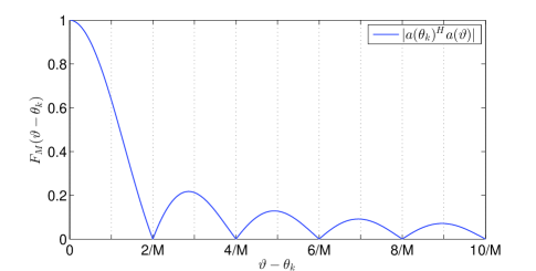
Figure 1: $F_{M}(\vartheta-\theta_{k})$ in (11) when $M=100$.

Thus, the rate of the RDB scheme for $K=1$ is insignificant regardless of the value of $M$. In this case, it is imperative to obtain the CSI of the single user to achieve the attainable rate of $\log(1+|\alpha_{1}|^{2}M)\sim_{M}\log M$ [1, 2, 3]. However, the situation becomes different as $K$ becomes large. In order to obtain an insight into the MU gain in the RDB scheme in mm-wave massive MIMO with the UR-LoS channel model before rigorous analysis in the next section, let us examine the relationship between $|{\bf a}(\theta_{k})^{H}{\bf a}(\vartheta)|$ and $\{\theta_{k},\vartheta\}$:

$$|{\bf a}(\theta_{k})^{H}{\bf a}(\vartheta)| =\frac{1}{M}\left|\sum_{n=0}^{M-1}e^{-\iota\pi n(\vartheta-\theta_{k})}\right|=\frac{1}{M}\left|\frac{1-e^{-\iota\pi(\vartheta-\theta_{k})M}}{1-e^{-\iota\pi(\vartheta-\theta_{k})}}\right|$$

$$=\frac{1}{M}\left|\frac{\sin\frac{\pi(\vartheta-\theta_{k})M}{2}}{\sin\frac{\pi(\vartheta-\theta_{k})}{2}}\right|=:F_{M}(\vartheta-\theta_{k}),$$ (11)

which is the Fejér kernel $F_{M}(\cdot)$ of order $M$ [19]. Fig. 1 shows the value of (11) versus $\vartheta-\theta_{k}$. From (11), we have $|{\bf a}(\theta_{k})^{H}{\bf a}(\vartheta)|\to 0$ as $M\to\infty$ for fixed $\vartheta$ and $\theta_{k}$. On the other hand, we have $|{\bf a}(\theta_{k})^{H}{\bf a}(\vartheta)|\to\left|\frac{2\sin\frac{\pi\Delta}{2}}{\pi\Delta}\right|$ as $M\to\infty$, provided that $\vartheta-\theta_{k}=\frac{\Delta}{M}$ for some $\Delta>0$ [17]. This is because

$$\frac{1}{M}\left|\frac{\sin\frac{\pi(\vartheta-\theta_{k})M}{2}}{\sin\frac{\pi(\vartheta-\theta_{k})}{2}}\right|\overset{(a)}{\approx}\frac{1}{M}\left|\frac{\sin\frac{\pi\Delta}{2}}{\frac{\pi\Delta}{2M}}\right|\to\left|\frac{2\sin\frac{\pi\Delta}{2}}{\pi\Delta}\right|$$ (12)

where $(a)$ holds from $\sin\epsilon\approx\epsilon$ for small $\epsilon>0$. That is, the asymptotic value of $|{\bf a}(\theta_{k})^{H}{\bf a}(\vartheta)|$ may not be zero if $(\vartheta-\theta_{k})$ becomes sufficiently small in the order of $O\left(\frac{1}{M}\right)$ as $M\to\infty$. On the other hand, one can show in a similar way that $|{\bf a}(\theta_{k})^{H}{\bf a}(\vartheta)|\to 0$ as $M\to\infty$, when $\vartheta-\theta_{k}=\frac{\Delta}{M^{\alpha}}$ for some $\alpha<1$ and $\Delta$.

Now, suppose that we can find a user $k$ such that $|\vartheta-\theta_{k}|<\frac{1}{M}$ almost surely due to MU diversity. Then, the rate ${\cal R}_{1}$ of the RDB scheme is lower bounded by

$${\cal R}_{1}\geq\mathbb{E}\left[\log\left(1+|\alpha_{k}|^{2}M\frac{4}{\pi^{2}}\right)\right]\sim_{M}\log M,$$ (13)

as $M\rightarrow\infty$. In other words, if the number $K$ of users as a function of $M$ is sufficiently large such that there exists a user $k$ for whom $|\vartheta-\theta_{k}|$ is sufficiently small in the order of $O\left(\frac{1}{M}\right)$ with high probability, the RDB scheme has asymptotically good performance.

IV Asymptotic Analysis of The RDB Rate: The Single Beam Case

In this section, we rigorously analyze the asymptotic performance of the RDB scheme in the single downlink beam case. Direct computation of ${\cal R}_{1}$ in (9) is difficult since the integral in (9) does not have a closed-form expression. To circumvent this difficulty, we use several techniques to bound ${\cal R}_{1}$ by first assuming that $\alpha_{k}=1$ for all $k$ and focusing on the term $Z_{k}:=M|{\bf a}(\theta_{k})^{H}{\bf a}(\vartheta)|^{2}$ in $\eqref{eq:expected_rate_s1}$. Then, we will include the term $\alpha_{k}\sim{\cal C}{\cal N}(0,1)$ in the performance analysis later. We begin with the following lemma.

Lemma 1

For any constant $p\in(-1,1)$ and sufficiently large $M$, we have

$$|\tilde{\theta}_{k}|<\frac{1}{\frac{\pi}{4}M^{(1+p)/2}}$$ (14)

under the event $\{Z_{k}>M^{p}\}$, and furthermore

$$\frac{1}{2\pi M^{(1+p)/2}}<\mathrm{Pr}\{Z_{k}>M^{p}\}<\frac{1}{\frac{\pi}{4}M^{(1+p)/2}},$$ (15)

where $\tilde{\theta}_{k}=\vartheta-\theta_{k}$ and $Z_{k}=M|{\bf a}(\theta_{k})^{H}{\bf a}(\vartheta)|^{2}$.

Proof: From (11), the event $\{Z_{k}=M|{\bf a}(\theta_{k})^{H}{\bf a}(\vartheta)|^{2}>M^{p}\}$ is equivalent to

$$\left|\frac{\sin\frac{\pi{\tilde{\theta}}_{k}M}{2}}{\sin\frac{\pi{\tilde{\theta}}_{k}}{2}}\right|>M^{(1+p)/2},$$ (16)

where ${\tilde{\theta}}_{k}\sim\mathrm{Unif}[-1,1]$ by Appendix A. A necessary condition to satisfy (16) is that the denominator in the left-hand side (LHS) of (16) should be upper bounded as

$$\left|\sin\frac{\pi{\tilde{\theta}}_{k}}{2}\right|<\frac{1}{M^{(1+p)/2}}$$ (17)

since the numerator $\left|\sin\frac{\pi{\tilde{\theta}}_{k}M}{2}\right|\leq 1$ and $M^{(1+p)/2}>1$ for $p\in(-1,1)$ and $M>1$. For given $p\in(-1,1)$, the upper bound in the right-hand side (RHS) of (17) goes to zero as $M\to\infty$. Hence, by the fact that $\frac{\epsilon}{2}<\sin\epsilon$ for small $\epsilon>0$, (17) implies

$$|{\tilde{\theta}}_{k}|<\frac{1}{\frac{\pi}{4}M^{(1+p)/2}}$$ (18)

for sufficiently large $M$. Therefore, (14) holds and we have the upper bound in (15), since (18) is a necessary condition for $\{Z_{k}>M^{p}\}$:

$$\mathrm{Pr}\{Z_{k}>M^{p}\}<\mathrm{Pr}\left\{|{\tilde{\theta}}_{k}|<\frac{1}{\frac{\pi}{4}M^{(1+p)/2}}\right\}=\frac{1}{\frac{\pi}{4}M^{(1+p)/2}}$$ (19)

for sufficiently large $M$, since $\tilde{\theta}_{k}\sim\mbox{Unif}[-1,1]$.

Now consider the lower bound in (15). From the fact that $\sin\epsilon<\epsilon$ for $\epsilon>0$, we have

$$\left|\sin\frac{\pi{\tilde{\theta}}_{k}}{2}\right|<\frac{1}{2M^{(1+p)/2}}$$ (20)

if

$$\frac{\pi}{2}|{\tilde{\theta}}_{k}|<\frac{1}{2M^{(1+p)/2}}.$$ (21)

If the following equation

$$\left|\sin\frac{\pi{\tilde{\theta}}_{k}M}{2}\right|\geq\frac{1}{2}$$ (22)

is satisfied in addition to (21) implying (20), then (16) is satisfied (i.e., the joint event of (21) and (22) is a sufficient condition for (16)). It is easy to see that the solution to (22) is

$$|{\tilde{\theta}}_{k}|\in\left\{\left[\frac{2k}{M}+\frac{1}{3M},\frac{2k}{M}+\frac{5}{3M}\right],k=0,1,2,\cdots,\right\}.$$ (23)

Note that $\left|\sin\frac{\pi{\tilde{\theta}}_{k}M}{2}\right|$ in (22) has period $\frac{2}{M}$ and the length of one interval per period contained in the set (23) is $\frac{4}{3M}$. Hence, the set (23) occupies $\frac{2}{3}$ length of each period of $\frac{2}{M}$. Since the term $\frac{1}{M^{(p+1)/2}}$ for given $p\in(-1,1)$ converges to zero slower than $\frac{1}{M}$ as $M\rightarrow\infty$, multiple discontinuous intervals in the set (23) are contained in the set defined by (21), and the length of the intersection of the sets (21) and (23) is lower bounded by $\frac{2}{3}\left(\frac{1}{\pi M^{(1+p)/2}}-\frac{2}{M}\right)$, where minus $\frac{2}{M}$ takes into account the impact of the last possibly partially overlapping interval. Hence, we have the lower bound part of (15):

$$\mathrm{Pr}\{Z_{k}>M^{p}\} \geq\frac{2}{3}\left(\frac{1}{\pi M^{(1+p)/2}}-\frac{2}{M}\right)>\frac{1}{2}\cdot\frac{1}{\pi M^{(1+p)/2}}.$$ (24)

for sufficiently large $M$. $\hfill\square$

Using Lemma 1 we have the following theorem.

Theorem 1

For $K=M^{q}$ and $q\in(0,1)$, we have asymptotic upper and lower bounds for ${\cal R}_{1}$ in (9) when $\alpha_{k}=1$ for all $k$, given by

$$\log(1+M^{2q-1-\epsilon})~{}\lesssim_{M}~{}\mathbb{E}\left[\log(1+Z)\right]~{}\lesssim_{M}~{}\log(1+M^{2q-1+\epsilon})$$ (25)

for any sufficiently small $\epsilon>0$, where $Z=\underset{1\leq k\leq K}{\max}Z_{k}$ and $x\lesssim_{M}y$ means $\lim_{M\to\infty}x/y\leq 1$.

Proof: The probability of the event $\{Z>M^{p}\}$ for any $p\in(-1,1)$ can be expressed as

$$\mathrm{Pr}\left\{\max_{k}Z_{k}>M^{p}\right\} =1-\mathrm{Pr}\{Z_{k}\leq M^{p}\}^{K}$$ (26)

$$=1-\left(1-\frac{1}{c_{M}M^{(1+p)/2}}\right)^{K},$$ (27)

where the second equality holds by (15) of Lemma 1 ($c_{M}$ is bounded between $\frac{\pi}{4}$ and $2\pi$ for all sufficiently large $M$). We consider the second term in (27). Pick $p=2q-1-\epsilon$ for small $\epsilon>0$ such that $p\in(-1,1)$. (For such $\epsilon$, $2q-\epsilon>0$.) Then the second term can be expressed as

$$\left(1-\frac{1}{c_{M}M^{(1+p)/2}}\right)^{K} =\left(1-\frac{1}{c_{M}M^{q-\frac{\epsilon}{2}}}\right)^{M^{q}}$$ (28)

$$=e^{M^{q}\log\left(1-\frac{1}{c_{M}M^{q-\frac{\epsilon}{2}}}\right)}$$ (29)

$$=e^{-\frac{1}{c_{M}}M^{\epsilon/2}+O\left(\frac{1}{M^{2q-\epsilon}}\right)}~{}\to 0~{}~{}\text{as}~{}~{}M\to\infty,$$ (30)

where we used the fact that $\log(1-x)=-x+O(x^{2})$ for small $x$ in the third step. Therefore, in this case, we have

$$\mathrm{Pr}\{Z>M^{p}\}\to 1,~{}~{}\text{as}~{}~{}M\to\infty$$ (31)

and thus $\mathbb{E}[\log(1+Z)]$ can be bounded as

$$\mathbb{E}[\log(1+Z)] \geq\int_{M^{p}}^{M}\log(1+z)p(z)dz$$ (32)

$$\geq\log(1+M^{p})\int_{M^{p}}^{M}p(z)dz$$ (33)

$$\sim_{M}\log(1+M^{p}),~{}~{}\text{as}~{}~{}M\to\infty,$$ (34)

since $\int_{M^{p}}^{M}p(z)dz=\mbox{Pr}\{Z>M^{p}\}\rightarrow 1$ in this case. Hence, the claim on the lower bound follows.

Now pick $p=2q-1+\epsilon$ for small $\epsilon>0$ such that $p\in(-1,1)$. (For such $\epsilon$, $2q+\epsilon>0$.) Then, by the techniques used in (28)-(30), the second term in (27) can be computed as

$$\left(1-\frac{1}{c_{M}M^{(1+p)/2}}\right)^{K} =e^{-\frac{1}{c_{M}}M^{-\epsilon/2}+O\left(\frac{1}{M^{2q+\epsilon}}\right)}$$ (35)

$$\stackrel{{\scriptstyle(a)}}{{=}}1+O\left(-\frac{1}{M^{\frac{\epsilon}{2}}}+\frac{1}{M^{2q+\epsilon}}\right)=1-O\left(\frac{1}{M^{\frac{\epsilon}{2}}}\right),$$ (36)

where the step (a) holds by the identity $e^{x}=1+O(x)$ for small $x$. Therefore, in this case, the probability of the event $\{Z>M^{p}\}$ is given by $O\left(\frac{1}{M^{\epsilon/2}}\right)$. Using this, we have

$$\mathbb{E}[\log(1+Z)] =\int_{M^{p}}^{M}\log(1+z)p(z)dz+\int_{0}^{M^{p}}\log(1+z)p(z)dz$$ (37)

$$\leq\log(1+M)O\left(\frac{1}{M^{\epsilon/2}}\right)+\log(1+M^{p})$$ (38)

$$\sim_{M}\log(1+M^{p}),~{}~{}\text{as}~{}~{}M\to\infty.$$ (39)

In the second step, we used $\int_{M^{p}}^{M}p(z)dz=\mbox{Pr}\{Z>M^{p}\}=O\left(\frac{1}{M^{\epsilon/2}}\right)$. Hence, the claim on the upper bound follows. $\hfill\square$

Theorem 1 states that the single-beam RDB scheme under the assumption $\alpha_{k}=1,~{}\forall~{}k$ has asymptotically nontrivial performance, i.e., ${\cal R}_{1}\to\infty$, as $M\rightarrow\infty$, when $K=M^{q}$ with $q\in(\frac{1}{2},1)$. On the other hand, when $K=M^{q}$ with $q\in(0,\frac{1}{2})$, the RDB scheme has trivial performance, i.e., ${\cal R}_{1}\to 0$, as $M\rightarrow\infty$. Thus, $q=\frac{1}{2}$ is the performance transition point for the single-beam RDB scheme under the UR-LoS channel model.

Now consider the impact of the path gain term $\alpha_{k}\overset{i.i.d.}{\sim}{\cal C}{\cal N}(0,1)$ on the single-beam RDB rate ${\cal R}_{1}$. In fact, the same is true under the assumption of $\alpha_{k}\overset{i.i.d.}{\sim}{\cal C}{\cal N}(0,1)$.

Theorem 2

For $K=M^{q}$ with $q\in(\frac{1}{2},1)$ and $\alpha_{k}\stackrel{{\scriptstyle i.i.d.}}{{\sim}}{\cal C}{\cal N}(0,1)$, we have

$$\lim_{M\to\infty}\frac{{\cal R}_{1}}{\mathbb{E}\left[\log(1+M\max_{k}|\alpha_{k}|^{2})\right]}=2q-1,$$ (40)

where ${\cal R}_{1}$ is the optimal single-beam RDB rate defined in (9) considering the random path gain, and $\mathbb{E}\left[\log(1+M\max_{k}|\alpha_{k}|^{2})\right]$ is the optimal rate of exact beamforming based on perfect CSI at the BS. On the other hand, when $q\in(0,\frac{1}{2})$, ${\cal R}_{1}\rightarrow 0$ as $M\rightarrow\infty$.

Proof: See Appendix B. $\hfill\square$

Note that the ratio $2q-1$ of the RDB rate ${\cal R}_{1}$ to the exact beamforming rate is the same for both assumptions $\alpha_{k}=1$ and $\alpha_{k}\sim{\cal C}{\cal N}(0,1)$. As seen, the single-beam RDB strategy achieves $2q-1$ fraction of the exact beamforming rate based on perfect CSI at the BS. The supremum fraction of one can be achieved arbitrarily closely when the number $K$ of users grows almost linearly w.r.t. $M$, i.e., $q$ is arbitrarily close to one.

Theorems 1 and 2 hold exactly in the same form when $K=c_{u}M^{q}$ for any constant $c_{u}>0$. However, for the notational simplicity in the proofs, we just used $K=M^{q}$. Note that in the single beam case we only have the power gain by the antenna array, as shown in the maximum rate of $\mathbb{E}\left[\log(1+M\max_{k}|\alpha_{k}|^{2})\right]$ even by perfect beamforming.

V Asymptotic Analysis of The RDB Rate: The Multiple Beam Case

In this section, we consider the case in which the number $S$ of randomly-directional beams is more than one and allowed to grow to infinity as a function of $M$, and analyze the corresponding asymptotic performance. In the multiple beam case, the BS transmits $S$ random beams equi-spaced in the normalized angle domain, defined as

$${\bf w}_{b}={\bf a}(\vartheta_{b})={\bf a}\left(\vartheta+\frac{2(b-1)}{S}\right),~{}~{}\text{for}~{}~{}b=1,\cdots,S,$$ (41)

where $\vartheta\sim\mathrm{Unif}[-1,1]$, to the downlink sequentially during the training period. We assume that the network is synchronized and thus each user knows the training beam index $b$ by the corresponding training interval. Here, the difference between the normalized directions of two adjacent beams is $\frac{2}{S}$ and the offset $\vartheta$ is randomly generated on $(-1,1]$. (Recall from (3) that ${\bf a}(\theta)$ is periodic in $\theta$ with period 2.) Note that the equi-spaced beams are asymptotically orthogonal to one another, i.e.,

$$\lim_{M\to\infty}|{\bf a}(\vartheta_{b_{1}})^{H}{\bf a}(\vartheta_{b_{2}})|=0~{}~{}\text{for}~{}~{}b_{1}\neq b_{2},$$ (42)

when $S=o(M)$.

In the next subsections, we analyze the asymptotic performance of single user selection based on multiple training beams first and multiple user selection based on multiple beams later.

V-A The Single User Selection Case

In the single user selection case, after the training period is over, each user reports the maximum of its received power values for the $S$ training beams and the corresponding beam index. Then, the BS transmits a data stream to the user that has maximum received power with the corresponding beam ${\bf w}_{b}$. In this case, the rate ${\cal R}_{S}$ is given by

$${\cal R}_{S}=\mathbb{E}\left[\log\left(1+\max_{1\leq k\leq K}\max_{1\leq b\leq S}|\alpha_{k}|^{2}M|{\bf a}(\theta_{k})^{H}{\bf a}(\vartheta_{b})|^{2}\right)\right].$$ (43)

First, consider the case of $|\alpha_{k}|=1$ for all $k=1,\cdots,K$ as before. In this case, we have the following theorem:

Theorem 3

For $K=M^{q}$, $S=M^{\ell}$ and any $\ell,q\in(0,1)$ such that $\ell+q<1$, we have asymptotic lower and upper bounds on ${\cal R}_{S}$ in the case of $|\alpha_{k}|=1,~{}\forall~{}k$, given by

$$\log(1+M^{2q+2\ell-1-\epsilon})~{}\lesssim_{M}~{}\mathbb{E}\left[\log(1+Z^{\prime})\right]~{}\lesssim_{M}~{}\log(1+M^{2q+2\ell-1+\epsilon})$$ (44)

for any sufficiently small $\epsilon>0$, where $Z^{\prime}=\max_{k}Z_{k}^{\prime}$ and $Z_{k}^{\prime}=\max_{b}M|{\bf a}(\theta_{k})^{H}{\bf a}(\vartheta_{b})|^{2}$.

Proof: Proof consists of two steps as in the proofs of Lemma 1 and Theorem 1: (i) first, we bound $\mathrm{Pr}\{Z_{k}^{\prime}\leq M^{p}\}$ and (ii) then bound $\mathbb{E}\left[\log(1+Z^{\prime})\right]$ using the bounds on $\mathrm{Pr}\{Z_{k}^{\prime}\leq M^{p}\}$.

(i) First, consider $\mathrm{Pr}\{A\}:=\mathrm{Pr}\{Z_{k}^{\prime}=\max_{b}M|{\bf a}(\theta_{k})^{H}{\bf a}(\vartheta_{b})|^{2}>M^{p}\}$ for $p\in(-1,1)$. Let $C_{i}$ be the event that $i=\arg\max_{b}M|{\bf a}(\theta_{k})^{H}{\bf a}(\vartheta_{b})|^{2}$, i.e., $C_{i}$ is the event that the $i$-th beam is the optimal beam for user $k$. Note that the distribution of $M|{\bf a}(\theta_{k})^{H}{\bf a}(\vartheta_{b})|^{2}=M\cdot F_{M}^{2}\left(\vartheta_{b}-\theta_{k}\right)=M\cdot F_{M}^{2}\left(\vartheta+\frac{2(b-1)}{S}-\theta_{k}\right)=M\cdot F_{M}^{2}\left({\tilde{\theta}}_{k}+\frac{2(b-1)}{S}\right)$ is independent of $b$ since ${\tilde{\theta}}_{k}=\vartheta-\theta_{k}\sim\mathrm{Unif}[-1,1]$ and the Fejér kernel $F_{M}({\tilde{\theta}})$ is a periodic function with period $2$. Hence, the events $C_{1},C_{2},\cdots,C_{M^{\ell}}$ are equally probable as $\mathrm{Pr}\{C_{i}\}=\frac{1}{S}=\frac{1}{M^{\ell}}$ for every $i=1,\cdots,M^{\ell}$. Furthermore, the conditional events $A|C_{1},A|C_{2},\cdots,A|C_{M^{\ell}}$ are also equally probable, i.e., $\mathrm{Pr}\{A|C_{1}\}=\cdots=\mathrm{Pr}\{A|C_{M^{\ell}}\}$ since the situation is the same for each $\vartheta_{b}$ due to the periodicity of $F_{M}(\cdot)$ of period two and ${\tilde{\theta}}_{k}\sim\mathrm{Unif}[-1,1]$. Hence, by the law of total probability and Bayes’ rule, we have

$$\mathrm{Pr}\{A\}=\sum_{i=1}^{M^{\ell}}\mathrm{Pr}\{A|C_{i}\}\mathrm{Pr}\{C_{i}\}=\mathrm{Pr}\{A|C_{1}\}=M^{\ell}\cdot\mathrm{Pr}\{A,C_{1}\}.$$

Thus, to bound $\mathrm{Pr}\{A\}$, we need to bound $\mathrm{Pr}\{A,C_{1}\}$. In order to bound $\mathrm{Pr}\{A,C_{1}\}$, we find a sufficient condition for the event $C_{1}$. Let $\tilde{C}_{1}(p)$ be the event $M|{\bf a}(\theta_{k})^{H}{\bf a}(\vartheta_{1})|^{2}>M^{p}$. Then, the event $\tilde{C}_{1}(p)$ with $p>2\ell-1$ implies

$$|\theta_{k}-\vartheta_{1}|\stackrel{{\scriptstyle(a)}}{{<}}\frac{1}{\frac{\pi}{4}M^{(p+1)/2}}\stackrel{{\scriptstyle(b)}}{{=}}\frac{1}{\frac{\pi}{4}M^{\ell+\delta/2}}$$ (45)

for sufficiently large $M$, where $\delta=p-(2\ell-1)>0$. (Here, step (a) is by (14) of Lemma 1 with $p\in(-1,1)$, and step (b) is by the new additional condition $p>2\ell-1$.) Therefore, in this case, $|\theta_{k}-\vartheta_{b}|>|\frac{2}{M^{\ell}}-\frac{1}{\frac{\pi}{4}M^{\ell+\delta/2}}|>\frac{1}{M^{\ell}}=\frac{1}{2}\frac{2}{S}$ for any $b\neq 1$ and sufficiently large $M$, and this implies for sufficiently large $M$

$$\tilde{C}_{1}(p)~{}\subset~{}C_{1}~{}~{}\text{for}~{}~{}p\in(-1,1)~{}\mbox{and}~{}p>2\ell-1.$$ (46)

Now consider $\mathrm{Pr}\{A,C_{1}\}$

$$\mathrm{Pr}\{A,C_{1}\} =\mathrm{Pr}\left\{\max_{b}M|{\bf a}(\theta_{k})^{H}{\bf a}(\vartheta_{b})|^{2}>M^{p},~{}1=\mathop{\arg\max}_{b}M|{\bf a}(\theta_{k})^{H}{\bf a}(\vartheta_{b})|^{2}\right\}$$

$$=\mathrm{Pr}\{\tilde{C}_{1}(p),C_{1}\}.$$ (47)

By using (46) and (47), we have

$$\mathrm{Pr}\{A,C_{1}\}\stackrel{{\scriptstyle(c)}}{{=}}\mathrm{Pr}\{\tilde{C}_{1}(p),C_{1}\}\stackrel{{\scriptstyle(d)}}{{=}}\mathrm{Pr}\{\tilde{C}_{1}(p)\}=\mathrm{Pr}\{M|{\bf a}(\theta_{k})^{H}{\bf a}(\vartheta_{1})|^{2}>M^{p}\}$$ (48)

when $p\in(-1,1)$ and $p>2\ell-1$ (these two conditions are required to apply (46) for step (d), and step (c) is valid by (47)). Now by applying (15) of Lemma 1 to the last term in (48) and using $\mathrm{Pr}\{A\}=M^{\ell}\cdot\mathrm{Pr}\{A,C_{1}\}$, we have for $p\in(-1,1)$ and $p>2\ell-1$,

$$\frac{1}{2\pi M^{(1+p-2\ell)/2}}<\mathrm{Pr}\{A\}<\frac{1}{\frac{\pi}{4}M^{(1+p-2\ell)/2}}.$$ (49)

(ii) Substituting $\mathrm{Pr}\{Z_{k}^{\prime}\leq M^{p}\}=1-\mathrm{Pr}\{A\}$ into $\mathrm{Pr}\{Z_{k}\leq M^{p}\}$ in (26) of the proof in Theorem 1 and following the proof of Theorem 1, we have for $p=2q+2\ell-1-\epsilon$ with arbitrarily small $\epsilon>0$,

$$\mathbb{E}[\log(1+Z^{\prime})]\gtrsim_{M}\log(1+M^{p}),$$ (50)

and for $p=2q+2\ell-1+\epsilon$ with arbitrarily small $\epsilon>0$,

$$\mathbb{E}[\log(1+Z^{\prime})]\lesssim_{M}\log(1+M^{p})$$ (51)

provided that $\ell+q<1$ (this is required for the condition $p\in(-1,1)$), where $x\gtrsim_{M}y$ indicates $\lim_{M\to\infty}x/y\geq 1$. Therefore, we have (44). $\hfill\square$

Corollary 1

For $K=M^{q}$, $S=M^{\ell}$ and any $\ell,q\in(0,1)$ such that $\frac{1}{2}<\ell+q<1$, we have

$$\lim_{M\to\infty}\frac{\mathbb{E}[\log(1+Z^{\prime})]}{\log(1+M)}=2(q+\ell)-1.$$ (52)

When the number $S$ of training beams is fixed, i.e., $\ell=0$, Corollary 1 reduces to the single beam result in (40). In the single user selection with multiple training beams, as seen in (52), the supremum of one for the achievable fraction can be achieved arbitrarily closely by the combination of multiple users $q$ and multiple training beams $\ell$. Thus, when there exist not sufficiently many users in the cell, multiple training beams can be used to enhance the RDB performance. Note that even for $q=0$, the optimal rate can be achieved with ${\cal R}_{S}$ by making $\ell\uparrow 1$, as expected. (In fact, this case corresponds to the case considered in the previous works on channel estimation for sparse mm-wave MIMO channels, e.g. [3].) Note also that the effect of two terms is not distinguishable at least in terms of the rate during the data transmission period, although multiple training beams require more training time. It can be shown that even with consideration of the random channel gain $\alpha_{k}\stackrel{{\scriptstyle i.i.d.}}{{\sim}}{\cal C}{\cal N}(0,1)$, the same result as (52) is valid.

V-B The Multiple User Selection Case: Multiplexing Gain

In this section, we consider multiple user selection with RDB with multiple beams, aiming at multiplexing gain, and investigate what can be achieved under the assumption of $|\alpha_{k}|=1,~{}\forall~{}k$ for simplicity. To do so, we consider a simple user scheduling method based on the RBF method [5] and then analyze the asymptotic performance of the considered scheduling method, which gives an achievable performance in the multi-beam multiple user selection case. The considered scheduling method is basically the RBF scheme in [5] with the $S$ random (asymptotically) orthogonal beams given by (41). That is, we choose a user that has maximum signal-to-interference-plus-noise ratio (SINR) for each beam ${\bf w}_{b}$, $b=1,\cdots,S$, defined in (41), and transmit $S$ independent data streams to the $S$ selected users. In this case, the received signal of a selected user $\kappa_{b}$ is given by

$$y_{\kappa_{b}}=\sqrt{\frac{P_{t}}{S}}{\bf h}_{\kappa_{b}}^{H}{\bf w}_{b}+\sqrt{\frac{P_{t}}{S}}\sum_{b^{\prime}\neq b}{\bf h}_{\kappa_{b}}^{H}{\bf w}_{b^{\prime}}+n_{\kappa_{b}},~{}~{}b=1,\cdots,S,$$ (53)

where $\kappa_{b}=\arg\max_{1\leq k\leq K}\mathrm{SINR}_{k,b}$, $\mathrm{SINR}_{k,b}=\frac{\rho M|{\bf a}(\theta_{k})^{H}{\bf a}(\vartheta_{b})|^{2}}{1+\sum_{b^{\prime}\neq b}\rho M|{\bf a}(\theta_{k})^{H}{\bf a}(\vartheta_{b^{\prime}})|^{2}}$, and $\rho=\frac{P_{t}}{S}$ is the per-user power of each scheduled user. The expected sum rate of this scheduling method is given by

$${\cal R}_{M}=\sum_{b=1}^{S}{\cal R}_{\kappa_{b}},$$ (54)

where the data rate of each scheduled user $\kappa_{b}$ for beam $b$ is given by

$${\cal R}_{\kappa_{b}}=\mathbb{E}\left[\log\left(1+\max_{1\leq k\leq K}\mathrm{SINR}_{k,b}\right)\right]=\mathbb{E}\left[\log\left(1+\frac{\rho M|{\bf a}(\theta_{\kappa_{b}})^{H}{\bf a}(\vartheta_{b})|^{2}}{1+\sum_{b^{\prime}\neq b}\rho M|{\bf a}(\theta_{\kappa_{b}})^{H}{\bf a}(\vartheta_{b^{\prime}})|^{2}}\right)\right].$$ (55)

We first introduce the following lemma necessary to derive the asymptotic result regarding (54) and (55):

Lemma 2

For $|{\tilde{\theta}}_{k}|\in(0,1]$, we have an upper bound for $F_{M}({\tilde{\theta}})$, given by $F_{M}({\tilde{\theta}}_{k})\leq\frac{1}{M|{\tilde{\theta}}_{k}|}$, where $F_{M}(\cdot)$ is defined in (11).

Proof: Since $F_{M}({\tilde{\theta}}_{k})$ and $\frac{1}{M|{\tilde{\theta}}_{k}|}$ are even functions, it is enough to consider ${\tilde{\theta}}_{k}\in(0,1]$ only. From (11), we have an upper bound of $F_{M}({\tilde{\theta}}_{k})$:

$$F_{M}({\tilde{\theta}}_{k}) \overset{(a)}{\leq}\frac{1}{M}\frac{1}{\sin\frac{\pi{\tilde{\theta}}_{k}}{2}}\overset{(b)}{\leq}\frac{1}{M{\tilde{\theta}}_{k}}$$

where $(a)$ follows from $|\sin\frac{\pi{\tilde{\theta}}_{k}M}{2}|\leq 1$ and $\sin\frac{\pi{\tilde{\theta}}_{k}}{2}>0$ for ${\tilde{\theta}}_{k}\in(0,1]$, and $(b)$ follows from

$$\frac{1}{{\tilde{\theta}}_{k}}-\frac{1}{\sin\frac{\pi{\tilde{\theta}}_{k}}{2}}\geq 0~{}~{}\Longleftrightarrow~{}~{}f({\tilde{\theta}}_{k}):=\sin\frac{\pi{\tilde{\theta}}_{k}}{2}-{\tilde{\theta}}_{k}\geq 0.$$

The RHS is true because $f(0)=f(1)=0$ with $f^{\prime\prime}({\tilde{\theta}}_{k})=-\frac{\pi^{2}}{4}\sin\frac{\pi{\tilde{\theta}}_{k}}{2}<0$ for ${\tilde{\theta}}_{k}\in(0,1]$. $\hfill\square$ Now the following theorem shows the asymptotic result on (54) and (55) when the total power $P_{t}$ is fixed regardless of $S$.

Theorem 4 (The case of fixed total transmit power $P_{t}=1$)

For $K=M^{q}$, $S=M^{\ell}$ with $q\in(0,1)$ and $\ell\in(0,q-\frac{\epsilon}{2})$, asymptotic upper and lower bounds on the per-user rate ${\cal R}_{\kappa_{b}}$ of selected user $\kappa_{b}$ for fixed total transmit power $P_{t}=1$ are given by

$$\log(1+M^{2q-1-\ell-\epsilon})\lesssim_{M}{\cal R}_{\kappa_{b}}\lesssim_{M}\log(1+M^{2q-1-\ell+\epsilon})$$ (56)

for any $\epsilon>0$.

Proof: The flow of proof is to first find lower and upper bounds on ${\cal R}_{\kappa_{b}}$, denoted by $L$ and $U$, respectively, and then to show that the bounds $L$ and $U$ are asymptotically bounded as

$$\log(1+M^{2q-1-\ell-\epsilon})\lesssim_{M}L\leq{\cal R}_{\kappa_{b}}\leq U\lesssim_{M}\log(1+M^{2q-1-\ell+\epsilon}).$$ (57)

To find $L$ and $U$, we consider a virtual user selection method based on maximizing signal power not SINR for each beam ${\bf a}(\vartheta_{b})$, i.e.,

$$\tilde{\kappa}_{b}=\mathop{\arg\max}_{1\leq k\leq K}M|{\bf a}(\theta_{k})^{H}{\bf a}(\vartheta_{b})|~{}~{}\text{for}~{}~{}b=1,\cdots,S.$$

Since the user $\tilde{\kappa}_{b}$ is chosen based on maximizing signal power only, we have $\mathrm{SINR}_{\tilde{\kappa}_{b},b}\leq\mathrm{SINR}_{\kappa_{b},b}$. Therefore, a lower bound on ${\cal R}_{\kappa_{b}}$ can be obtained as

$${\cal R}_{\kappa_{b}}\geq{\cal R}_{\tilde{\kappa}_{b}}=\mathbb{E}\left[\log\left(1+\frac{\rho Z_{bb}}{1+\rho\sum_{b^{\prime}\neq b}Z_{bb^{\prime}}}\right)\right]=:L$$ (58)

where $Z_{bb^{\prime}}:=M|{\bf a}(\theta_{\tilde{\kappa}_{b}})^{H}{\bf a}(\vartheta_{b^{\prime}}))|^{2}$ for $b^{\prime}=1,\cdots,S$. Furthermore, an upper bound on ${\cal R}_{\kappa_{b}}$ can be obtained by simply ignoring the inter-beam interference as

$${\cal R}_{\kappa_{b}}\leq\mathbb{E}[\log(1+\rho M|{\bf a}(\theta_{\kappa_{b}})^{H}{\bf a}(\vartheta_{b})|^{2})]\leq\mathbb{E}[\log(1+\rho Z_{bb})]=:U.$$ (59)

By modifying Theorem 1 to include $\rho=1/S=M^{-\ell}$ in front of $Z_{bb}$ and applying the modified theorem to $U$ in (59), we obtain

$$U\lesssim_{M}\log(1+M^{2q-1-\ell+\epsilon}).$$ (60)

Hence, the claim on the upper bound follows.

Now consider the case of lower bound $L$. From the fact that $\mathbb{E}[f(X)]=\int f(x)p(x)dx\geq\int f(x)p(x,A)dx=p(A)\mathbb{E}[f(X|A)]$ for a non-negative function $f(X)$, $L$ in (58) with $\rho=1/S=M^{-\ell}$ can be bounded as

$$\mathbb{E}\left[\log\left(1+\frac{M^{-\ell}Z_{bb}}{1+M^{-\ell}\sum_{b^{\prime}\neq b}Z_{bb^{\prime}}}\right)\right]$$

$$~{}~{}\geq\mathrm{Pr}\{Z_{bb}\geq M^{p}\}\cdot\mathbb{E}\left[\log\left(1+\frac{M^{-\ell}Z_{bb}}{1+M^{-\ell}\sum_{b^{\prime}\neq b}Z_{bb^{\prime}}}\right)\bigg{|}Z_{bb}\geq M^{p}\right].$$ (61)

Under the condition that $\{Z_{bb}\geq M^{p}\}$, we have

$$|\theta_{\tilde{\kappa}_{b}}-\vartheta_{b}|\leq\frac{1}{\frac{\pi}{4}M^{(1+p)/2}}$$

by (14) of Lemma 1. Therefore, $|\theta_{\tilde{\kappa}_{b}}-\vartheta_{b^{\prime}}|>\left|\frac{2}{S}-\frac{1}{\frac{\pi}{4}M^{(1+p)/2}}\right|$, $\forall b^{\prime}\neq b$. Furthermore, we can re-arrange the indices of $\{\vartheta_{b^{\prime}}\}_{b^{\prime}\neq b}$ in the order of closeness to $\vartheta_{b}$ with the new indices $\{j\}$. Then, we have

$$|\theta_{\tilde{\kappa}_{b}}-\vartheta_{2j-1}|,|\theta_{\tilde{\kappa}_{b}}-\vartheta_{2j}|>\left|\frac{2j}{M^{\ell}}-\frac{1}{\frac{\pi}{4}M^{(1+p)/2}}\right|,$$ (62)

since $\frac{2}{S}=\frac{2}{M^{\ell}}$ is the angular spacing between two adjacent beams. We now have a lower bound on $L$, given by

$$L \overset{(a)}{\geq}\mathrm{Pr}\{Z_{bb}\geq M^{p}\}\cdot\mathbb{E}\left[\log\left(1+\frac{M^{-\ell}Z_{bb}}{1+M^{-\ell}\sum_{j\neq b}\frac{1}{M|\theta_{\tilde{\kappa}_{b}}-\vartheta_{j}|^{2}}}\right)\bigg{|}Z_{bb}\geq M^{p}\right]$$

$$\overset{(b)}{\geq}\mathrm{Pr}\{Z_{bb}\geq M^{p}\}\cdot\mathbb{E}\left[\log\left(1+\frac{M^{-\ell}Z_{bb}}{1+M^{-\ell}\sum_{j=1}^{\frac{S}{2}}\frac{2}{M\left|\frac{2j}{S}-\frac{1}{\frac{\pi}{4}M^{(1+p)/2}}\right|^{2}}}\right)\bigg{|}Z_{bb}\geq M^{p}\right]$$

$$\overset{(c)}{\gtrsim}_{M}\mathrm{Pr}\{Z_{bb}\geq M^{p}\}\cdot\mathbb{E}\left[\log\left(1+\frac{M^{-\ell}Z_{bb}}{1+2M^{\ell-1}\sum_{j=1}^{\frac{S}{2}}\frac{1}{j^{2}}}\right)\bigg{|}Z_{bb}\geq M^{p}\right]$$

$$\overset{(d)}{\geq}\mathrm{Pr}\{Z_{bb}\geq M^{p}\}\cdot\log\left(1+\frac{M^{-\ell}M^{p}}{1+\frac{\pi^{2}M^{\ell-1}}{3}}\right)$$

$$\sim_{M}\log(1+M^{p-\ell}),$$ (63)

where $(a)$ holds by (61) and Lemma 2 with $Z_{bj}=MF_{M}^{2}(\theta_{\tilde{\kappa}_{b}}-\vartheta_{j})$; $(b)$ holds by (62); $(c)$ holds because $\left|\frac{2j}{M^{\ell}}-\frac{1}{\frac{\pi}{4}M^{(1+p)/2}}\right|^{2}\gtrsim_{M}\left|\frac{j}{M^{\ell}}\right|^{2}$ for large $M$ provided that $\ell<(1+p)/2$; $(d)$ follows from $\sum_{j=1}^{\infty}\frac{1}{j^{2}}=\frac{\pi^{2}}{6}$; and the last step holds because $\mathrm{Pr}\{Z_{bb}\geq M^{p}\}\to 1$ for $p<2q-1$ by (31) and $\frac{\pi^{2}M^{\ell-1}}{3}\to 0$ for $\ell<1$. Hence the claim on the lower bound follows.

Note that the conditions used to derive (63) and (60) are $p<2q-1$, $\ell<(1+p)/2$, and $\ell<1$, and $q$ and $\ell$ are given. Set $p=2q-1-\epsilon$ for $\epsilon>0$. Then, $\ell<q-\epsilon/2<1$ since $q\in(0,1)$. This concludes proof. $\hfill\square$

Theorem 5 (The case of fixed per-user power $\rho=1$, i.e. $P_{t}=S$)

For $K=M^{q}$ and $S=M^{\ell}$ with $q\in(0,1)$ and $\ell\in(0,\min(q-\frac{\epsilon}{2},\frac{1}{2}))$, asymptotic upper and lower bounds on the per-user rate ${\cal R}_{\kappa_{b}}$ of selected user $\kappa_{b}$ for $\rho=1$ are given by

$$\log(1+M^{2q-1-\epsilon})\lesssim_{M}{\cal R}_{\kappa_{b}}\lesssim_{M}\log(1+M^{2q-1+\epsilon})$$ (64)

for any $\epsilon>0$.

Proof: Proof is similar to that of Theorem 4 and omitted due to space limitation. $\hfill\square$

In Theorems 4 and 5, the condition $\ell<q-\epsilon/2<1$ guarantees that the $S$ beams are asymptotically orthonormal by (42) and there exist more users than the number of beams in the cell by the difference in the fractional orders $q$ and $\ell$. First, note that the per-user rate in Theorem 5 is the same as that in Theorem 1, i.e., the same per-user rate as that of the single beam case can be achieved in the multi-beam multi-user selection case when per-user power is fixed and the same. Now consider the sum rate in the multiple beam multi-user selection case. The sum rate ${\cal R}_{M}$ corresponding to Theorem 4 behaves as ${\cal R}_{M}=\Theta(M^{\ell}\log M^{2q-1-\ell})$ when $2q-1-\ell>0$. Pick $\ell=1-\delta_{1}$ for some small $\delta_{1}>0$ and pick $q=\ell+\epsilon/2+\delta_{2}$ for some small $\delta_{2}>0$ such that $\delta_{1}-\delta_{2}-\epsilon/2>0$ to have $q<1$ and $-\delta_{1}+2\delta_{2}+\epsilon>0$ to have $2q-1-\ell>0$. Then, we have $M^{\ell}\log M^{2q-1-\ell}=M^{1-\delta_{1}}\log(M^{-\delta_{1}+2\delta_{2}+\epsilon})$. Thus, sum rate behavior arbitrarily close to linear scaling w.r.t. the number of antennas is possible in the multi-beam multi-user selection case by random beamforming (randomly-directional beamforming) with proper user scheduling under the UR-LoS channel model. This is a significant difference from the sum rate behavior (7) of the RBF method [5] in large-scale MIMO, i.e., $\lim_{K\rightarrow\infty}\frac{\log K}{M}=0$, under the i.i.d. Rayleigh fading channel model (5) representing rich scattering environments. The major performance difference results from the difference in degrees-of-freedom in the two channels: the UR-LoS channel (4) and the i.i.d. Rayleigh fading channel (5). In the i.i.d. Rayleigh fading channel case, we have $M$ independent parameters and the channel vector is randomly located within a ball in the $M$-dimensional space. Consider a cone around each axis in the $M$-dimensional space so that channel vectors each of which is contained in each of the cones are roughly orthogonal, as shown in Fig. 3 of [12]. Then, the probability that a channel vector generated randomly according to (5) falls into such a cone is exponentially decreasing as $M$ increases (See Appendix C). Hence, if the number $K$ of users randomly distributed within the ball does not increases exponentially fast w.r.t. the dimension $M$ (i.e., $\lim_{K\rightarrow\infty}\frac{\log K}{M}=0$), it is difficult to find $M$ users whose channel vectors are contained in the $M$ roughly-orthogonal cones (one for each) [5, 7, 9] (the goal of SUS [6], RBF [5] or ReDOS-PBR [12] scheduling is to find such $M$ users), and linear sum rate scaling by random beamforming w.r.t. the dimension $M$ (i.e., the number of antennas) is not attainable. In the considered mm-wave MIMO with the UR-LoS channel model, however, the situation is quite different. Theorems 4 and 5 state that sum rate scaling arbitrarily close to linear scaling w.r.t. $M$ is possible in this case. This is because the degree-of-freedom in the UR-LoS channel model (4) with $\alpha_{k}=1$ is one regardless of the value of $M$. The orthogonality of the multiple transmit beams is attained by simply dividing the line of the normalized angle $\theta$ with length 2 by line segments each with length $2/S=2/M^{\ell}$. Thus, if $K=M^{q}$ with $q>\ell$, there exists many users in each line segment one of which is well matched to the transmit beam direction associated with each line segment if $2q-1-\ell>0$. Thus, in this case user scheduling to select such $S$ users is beneficial for random beamforming-based BS operation. In fact, the channel matrix composed of the channel vectors of the users scheduled in such a way satisfies the asymptotically favorable propagation condition in [17]. Note that the fundamental difference between the UR-LoS channel (4) modeling high propagation directivity and the i.i.d. Rayleigh fading channel model (5) for rich scattering is that linear sum rate scaling w.r.t. the number $M$ of antennas by random beamforming is attainable with the number $K$ of users increasing linearly w.r.t. $M$ in the UR-LoS channel model, whereas linear sum rate scaling w.r.t. the number $M$ of antennas by random beamforming is attainable with $K$ increasing exponentially w.r.t. $M$ in the i.i.d. Rayleigh fading channel model! Thus, high directivity is preferred to rich scattering for opportunistic random beamforming under massive MIMO situation. This suggests that opportunistic random beamforming is a viable choice for massive MIMO in the mm-wave band with high propagation directivity.

V-C Performance comparison: The fractional rate order

In this subsection, we compare the asymptotic performance of the three schemes considered in the previous sections. Here, we assume $\alpha_{k}=1,~{}\forall~{}k$ and $P_{t}=1$. In order to compare the relative performance, we define the fractional rate order (FRO) $\gamma$ as

$$\gamma:=\lim_{M\to\infty}\frac{\log{\cal R}}{\log M}.$$ (65)

Note that ${\cal R}=\Theta(M^{\gamma})$ for $\gamma\neq 0$. For $\gamma>0$, ${\cal R}$ increases to infinity as $M\rightarrow\infty$, whereas for $\gamma<0$, ${\cal R}$ decreases to zero as $M\rightarrow\infty$. Now consider the three rates ${\cal R}={\cal R}_{1},{\cal R}_{S}$, and ${\cal R}_{M}$. First, for the single beam RDB rate ${\cal R}_{1}$ we have by Theorem 1 that

$$\gamma_{1}=\lim_{M\to\infty}\frac{\log{\cal R}_{1}}{\log M}=\left\{\begin{array}[]{ll}0,&~{}\text{for}~{}q\in(\frac{1}{2},1)\\ 2q-1&~{}\text{for}~{}q\in(0,\frac{1}{2}),\end{array}\right.$$ (66)

where we used $\log(1+x)=x$ for small $x$ for the second part. Next, for the multi-beam RDB scheme with single-user selection, we have

$$\gamma_{S}=\lim_{M\to\infty}\frac{\log{\cal R}_{S}}{\log M}=0,~{}~{}\text{for}~{}~{}q\in(0,1)$$ (67)

by Theorem 3 with setting $\ell$ such that $1/2<\ell+q<1$. Here, $\gamma_{S}=0$ is achieved even for $q\in(0,1/2)$ because of added $\ell$. Finally, we consider the multi-beam RDB strategy with multi-user selection. In this case, ${\cal R}_{M}=\Theta(M^{\ell}\log(1+M^{2q-\ell-1}))$ from Theorem 4 and (54). Using $M^{\ell}\log(1+M^{2q-\ell-1})=\log(1+1/M^{-2q+\ell+1})^{M^{\ell}M^{-2q+\ell+1-(-2q+\ell+1)}}=\log(1+\frac{1}{M^{-2q+\ell+1}})^{M^{-2q+\ell+1}M^{2q-1}}\sim_{M}M^{2q-1}$ by setting $\ell$ such that $2q-1<\ell<q$, we obtain

$$\lim_{M\to\infty}\frac{\log{\cal R}_{M}}{\log M}=2q-1,~{}~{}\text{for}~{}~{}q\in(0,1).$$ (68)

\psfrag{1}[c]{\large$1$}\psfrag{-1}[c]{\large$-1$}\psfrag{q}[c]{ \large$q$}\psfrag{p}[r]{ \large$\underset{M\to\infty}{\lim}\frac{\log{\cal R}}{\log M}$ }\psfrag{h}[c]{\large$\frac{1}{2}$}\psfrag{0}[c]{\large$0$}\psfrag{r1}[l]{\large${\cal R}={\cal R}_{1}$}\psfrag{rs}[l]{\large${\cal R}={\cal R}_{S}$}\psfrag{rm}[l]{\large${\cal R}={\cal R}_{M}$}\epsfbox{figures/perf_region2.eps}

Figure 2: Fractional rate order versus $q$

Fig. 2 shows (66), (67) and (68) versus $q\in(0,1)$, and shows which strategy among RDB should be used for different $q$ determining the number of users in the cell relative to the number of antenna elements. ${\cal R}_{M}$ has the largest FRO for $q\in(\frac{1}{2},1)$, whereas ${\cal R}_{S}$ has the largest FRO for $q\in(0,\frac{1}{2})$. $\gamma_{1}$ is a lower bound on both $\gamma_{S}$ and $\gamma_{M}$ for all $q\in(0,1)$, and $\gamma_{M}\uparrow 1$ as $q\uparrow 1$, as mentioned already. Note that $\gamma_{M}<0$ for $q\in(0,\frac{1}{2})$, which implies ${\cal R}_{M}\rightarrow 0$ as $M\rightarrow\infty$. This is because the total number of users in the cell is not sufficient to find a user well matched to each beam. The transition point of determining the scarcity of users in the cell is $K=\Theta(\sqrt{M})$ under the UR-LoS model, whereas the transition point is $K=\Theta(\exp(\eta^{2}M))$ for some $\eta^{2}\in(0,1)$ or equivalently $M=\Theta(\log K)$ in the i.i.d. Rayleigh fading channel model. When $q\in(0,1/2)$, i.e., there exist not many users in the cell, the best strategy is the multi-beam single-user strategy. This implies that downlink channel estimation to identify the user channel, i.e., user’s propagation angle is important in this regime. On the other hand, when $q\in(1/2,1)$, i.e., there exist a sufficient number of users in the cell, downlink channel estimation is less important, and user scheduling based on equi-spaced random beams with an arbitrary angle offset is sufficient to obtain good performance and achieves linear sum rate scaling w.r.t. the number of antennas when the number of users increases linearly w.r.t. the number of antennas.

VI Numerical results

In this section, we provide some numerical results to validate our asymptotic analysis in the previous sections. All the expectations in the below are average over 5000 channel realizations and we set to $P_{t}=1$.

VI-A The Single Beam Case

To verify the asymptotic analysis in Section IV, we considered a mm-wave MU-MISO downlink system with the UR-LoS channel model. Fig. 3 (a) and (b) shows the value of $\frac{\mathbb{E}[1+Z]}{\log(1+M)}$ versus $q$ for $M=100,500,1000,5000,10000$ for $\alpha_{k}=1$ and $\alpha_{k}\sim{\cal C}{\cal N}(0,1)$, respectively. It is seen that the curve of $\frac{\mathbb{E}[1+Z]}{\log(1+M)}$ versus $q$ gradually converges to the theoretical line of $2q-1$ for $q>\frac{1}{2}$ and $0$ for $q\leq\frac{1}{2}$ as $M$ increases. Note that there exist some gap between the theoretical asymptotic line and the finite-sample results. This results from the slow rate of convergence.

(a) (b)

Figure 3: The ratio of the RDB rate ${\cal R}_{1}$ to the rate with perfect CSI $\mathbb{E}[\log(1+\max_{k}|\alpha_{k}|^{2}M)]$ versus $q$ for different $M$: (a) $\alpha_{k}=1$ and (b) $\alpha_{k}\sim{\cal C}{\cal N}(0,1)$

Fig. 4 (a) and (b) show the actual RDB rate w.r.t. $M$ for $q=0.1$ to $0.5$ and $q=0.6$ to $1$, respectively, in the case of $\alpha_{k}\sim{\cal C}{\cal N}(0,1)$. It is seen in Fig. 4 (a) that the RDB rate for $q$ below $0.5$ decreases as $M$ increases, but it almost remains the same when $q=0.5$. On the other hand, it is seen in Fig. 4 (b) that the RDB rate for $q$ above $0.5$ increases as $M$ increases. (Since x-axis is in log scale, the rate curve is linear as expected by Theorem 2 when $q>0.5$.) The results in Figs. 3 and 4 coincide with Theorems 1 and 2.

(a) (b)

Figure 4: The RDB rate ${\cal R}_{1}$ versus $M$ with $\alpha_{k}\sim{\cal C}{\cal N}(0,1)$ for different $q$ (log scale on x-axis): (a) $q=0.1,0.2,\cdots,0.5$ and (b) $q=0.6,0.7,\cdots,1$

VI-B The Multiple Beam Case

We first considered the multiple beam RDB with single user selection. Fig. 5 (a) and (b) show the ratio of the multiple beam RDB rate ${\cal R}_{S}$ with single-user selection to the rate with perfect CSI versus $q$ for different $\ell$ in the cases of $\alpha_{k}=1$ and $\alpha_{k}\sim{\cal C}{\cal N}(0,1)$, respectively, when $M=1000$. It is seen that the simulation curves roughly match the theoretical lines.

(a) (b)

Figure 5: The ratio of ${\cal R}_{S}$ to the rate with perfect CSI $\mathbb{E}[\log(1+\max_{k}|\alpha_{k}|^{2}M)]$ versus $q$ for different $\ell$: (a) $\alpha_{k}=1,\forall k$ and (b) $\alpha_{k}\sim{\cal C}{\cal N}(0,1),\forall k$

We then verified the rate ${\cal R}_{S}$ for $q=0.3$ with different $\ell$. It is seen in Fig. 6 (a) that ${\cal R}_{S}$ increases as $M$ increases for the cases of $\ell>0.2$ (i.e., $q+\ell>0.5$), as predicted by Theorem 3. On the other hand, the rate decreases for the case of $\ell<0.2$ as $M$ increases. Finally, we verified the multi-beam multi-user selection RDB. We set to $q=0.7$ and used $\alpha_{k}\sim{\cal C}{\cal N}(0,1)$, $\forall~{}k$. Fig. 6 (b) shows the per-user rate ${\cal R}_{\kappa_{b}}$ in Theorem 4 versus $M$ for different $\ell$. It is seen that the per-user rate ${\cal R}_{\kappa_{b}}$ increases when $\ell<0.4$, whereas it decreases when $\ell>0.4$, as $M$ increases, as predicted by Theorem 4 (i.e., $2q-1-\ell>0$ or $2q-1-\ell<0$).

(a) (b)

Figure 6: (a) ${\cal R}_{S}$ versus $M$ ($q=0.3$ and $\alpha_{k}\sim{\cal C}{\cal N}(0,1)$) (log scale on x-axis) and (b) the per-user rate of the multi-beam multi-user selection RDB versus $M$ ($q=0.7$ and $\alpha_{k}\sim{\cal C}{\cal N}(0,1)$)

VII Conclusion

We have considered RDB for millimeter-wave MU-MISO and examined the associated MU gain, using asymptotic performance analysis based on the UR-LoS channel model which well captures radio propagation channels in the mm-wave band. We have shown that there exists a transition point on the number of users relative to the number of antenna elements for non-trivial performance of the RDB scheme and have identified the case in which downlink training and channel estimation are important for good performance. We have also shown that sum rate scaling arbitrarily close to linear scaling w.r.t. the number of antenna elements can be achieved under the UR-LoS channel model by random beamforming based on multiple beams equi-spaced in the angle domain and proper user scheduling, if the number of users in the cell increases linearly w.r.t. the number of antenna elements. We have compared three RDB schemes composed of beamforming and user scheduling based on the newly defined fractional rate order, yielding insights into the most effective beamforming and scheduling choices for mm-wave MU-MISO in various operating conditions. Simulation results validate the analysis based on asymptotic techniques for finite cases. The results here is based on the simplified UR-LoS channel model capturing high propagation directivity, and thus extension to a general channel model is left as future work.

Appendix A Distribution of $\vartheta-\theta_{k}$

Since $\vartheta,\theta_{k}\overset{\text{i.i.d.}}{\sim}\mathrm{Unif}[-1,1]$, the difference random variable ${\tilde{\theta}}_{k}$ has the distribution, given by

$$p({\tilde{\theta}})=\left\{\begin{array}[]{ll}\frac{1}{4}{\tilde{\theta}}+\frac{1}{2},&-2\leq{\tilde{\theta}}\leq 0\\ -\frac{1}{4}{\tilde{\theta}}+\frac{1}{2},&~{}~{}0\leq{\tilde{\theta}}\leq 2.\\ \end{array}\right.$$ (69)

For any function $f(\tilde{\theta})$ with the periodicity of period two, we have $f(\tilde{\theta})=f(\tilde{\theta}+2)$ for $\tilde{\theta}\in[-1,0]$ and $f(\tilde{\theta})=f(\tilde{\theta}-2)$ for $\tilde{\theta}\in[0,1]$. Therefore, we can regard $p(\tilde{\theta})$ on the function $f(\tilde{\theta})$ as

$$p(\tilde{\theta})=\left\{\begin{array}[]{ll}\frac{1}{4}\tilde{\theta}+\frac{1}{2}-\frac{1}{4}\tilde{\theta},&~{}-1\leq\tilde{\theta}\leq 0\\ -\frac{1}{4}\tilde{\theta}+\frac{1}{2}+\frac{1}{4}\tilde{\theta},&~{}~{}~{}~{}0\leq\tilde{\theta}\leq 1\end{array}\right.$$ (70)

i.e., $\tilde{\theta}\sim\mathrm{Unif}[-1,1]$.

Appendix B Proof of Theorem 2

Before proving Theorem 2, we prove another interesting lemma of which proof is partly used in proof of Theorem 2.

Lemma 3

For $K=M^{q}$, $q\in(\frac{1}{2},1)$ and $\alpha_{k}\overset{\text{i.i.d.}}{\sim}{\cal C}{\cal N}(0,1)$, we have

$$\lim_{M\to\infty}\frac{{\cal R}_{1}}{\mathbb{E}\left[\log(1+|\alpha_{k^{\prime}}|^{2}Z_{k^{\prime}})\right]}=1,$$ (71)

where $k^{\prime}=\arg\max_{k}Z_{k}$, and ${\cal R}_{1}$ is the optimal RDB rate in (9) considering the random path gain.

Proof: ${\cal R}_{1}$ is bounded as

$$\mathbb{E}[\log(1+|\alpha_{k^{\prime}}|^{2}Z_{k^{\prime}})]\leq{\cal R}_{1}\leq\mathbb{E}\left[\log\left(1+\left(\max_{k}|\alpha_{k}|^{2}\right)Z_{k^{\prime}}\right)\right].$$ (72)

Eq. (25) in Theorem 1 can easily be modified to

$$\log(1+\beta M^{2q-1-\epsilon})~{}\lesssim_{M}~{}\mathbb{E}\left[\log(1+\beta Z)\right]~{}\lesssim_{M}~{}\log(1+\beta M^{2q-1+\epsilon})$$ (73)

for $q\in(\frac{1}{2},1)$ and $\beta>0$. Note that $\mathbb{E}[\log(1+|\alpha_{k^{\prime}}|^{2}Z_{k^{\prime}})]=\mathbb{E}[\mathbb{E}[\log(1+|\alpha_{k^{\prime}}|^{2}Z_{k^{\prime}})~{}|~{}|\alpha_{k^{\prime}}|^{2}]]$ by the law of iterated expectations. Applying the lower bound in (73) to $\mathbb{E}[\log(1+|\alpha_{k^{\prime}}|^{2}Z_{k^{\prime}})~{}|~{}|\alpha_{k^{\prime}}|^{2}]$, we have

$$\mathbb{E}[\log(1+|\alpha_{k^{\prime}}|^{2}M^{2q-1-\epsilon})]\lesssim_{M}\mathbb{E}[\log(1+|\alpha_{k^{\prime}}|^{2}Z_{k^{\prime}})].$$ (74)

For $q\in(\frac{1}{2},1)$, we have

$$\mathbb{E}[\log(1+|\alpha_{k^{\prime}}|^{2}M^{2q-1-\epsilon})] \sim_{M}\mathbb{E}[\log(|\alpha_{k^{\prime}}|^{2}M^{2q-1-\epsilon})]$$

$$=\mathbb{E}[\log|\alpha_{k^{\prime}}|^{2}]+(2q-1-\epsilon)\log M$$

$$\sim_{M}(2q-1-\epsilon)\log M$$ (75)

for any sufficiently small $\epsilon>0$ such that $2q-1-\epsilon>0$. Since $|\alpha_{k^{\prime}}|^{2}\sim\chi^{2}(2)$, $\mathbb{E}[\log|\alpha_{k^{\prime}}|^{2}]$ is a constant.

Now consider the upper bound in (72). Again applying the law of iterated expectations and the upper bound in (73), we have $\mathbb{E}\left[\log\left(1+\left(\max_{k}|\alpha_{k}|^{2}\right)Z_{k^{\prime}}\right)\right]\leq\mathbb{E}\left[\log\left(1+\left(\max_{k}|\alpha_{k}|^{2}\right)M^{2q-1+\epsilon}\right)\right]$. From the fact that $\mathbb{E}[\log(1+\max_{k}|\alpha_{k}|^{2})]\sim_{M}\log(\log K)$ [5], the above bound can further be simplified as

$$\mathbb{E}\left[\log\left(1+\left(\max_{k}|\alpha_{k}|^{2}\right)Z_{k^{\prime}}\right)\right] \lesssim_{M}\log(M^{2q-1+\epsilon}\log K)$$

$$\sim_{M}(2q-1+\epsilon)\log M+\log(\log M).$$ (76)

Dividing (72) by $\mathbb{E}[\log(1+|\alpha_{k^{\prime}}|^{2}Z_{k^{\prime}})]$, we have

$$1\leq\frac{{\cal R}_{1}}{\mathbb{E}[\log(1+|\alpha_{k^{\prime}}|^{2}Z_{k^{\prime}})]} \leq\frac{\mathbb{E}\left[\log\left(1+\left(\max_{k}|\alpha_{k}|^{2}\right)Z_{k^{\prime}}\right)\right]}{\mathbb{E}[\log(1+|\alpha_{k^{\prime}}|^{2}Z_{k^{\prime}})]}$$

$$\overset{(a)}{\lesssim}_{M}\frac{(2q-1+\epsilon)\log M+\log\log M}{(2q-1-\epsilon)\log M}$$

$$\sim_{M}\frac{2q-1+\epsilon}{2q-1-\epsilon}$$ (77)

where step $(a)$ follows from (75) and (76). Since (77) holds for any small $\epsilon>0$, the claim follows. $\hfill\square$

Proof of Theorem 2:     By (72), (75), and (76), we have

$$(2q-1-\epsilon)\log M\lesssim_{M}{\cal R}_{1}\lesssim_{M}(2q-1+\epsilon)\log M+\log\log M.$$

Dividing the above equation by $\mathbb{E}[\log(1+M\max_{k}|\alpha_{k}|^{2})]$ and using the fact that $\mathbb{E}[\log(1+M\max_{k}|\alpha_{k}|^{2})]\sim_{M}\log M+\log\log M$ [5], we have

$$\frac{(2q-1-\epsilon)\log M}{\log M+\log\log M}\lesssim_{M}\frac{{\cal R}_{1}}{\mathbb{E}[\log(1+M\max_{k}|\alpha_{k}|^{2})]}\lesssim_{M}\frac{(2q-1+\epsilon)\log M+\log\log M}{\log M+\log\log M}$$

for arbitrarily and sufficiently small $\epsilon>0$. Hence, we have

$$2q-1-\epsilon\lesssim_{M}\frac{{\cal R}_{1}}{\mathbb{E}[\log(1+M\max_{k}|\alpha_{k}|^{2})]}\lesssim_{M}2q-1+\epsilon.$$ (78)

Now consider the case of $q\in(0,\frac{1}{2})$. In this case, Eq. (25) in Theorem 1 can be modified to

$$\beta M^{2q-1-\epsilon}\lesssim_{M}\mathbb{E}[\log(1+\beta Z)]\lesssim_{M}\beta M^{2q-1+\epsilon}$$ (79)

for $\beta>0$ and sufficiently small $\epsilon>0$ such that $2q-1+\epsilon<0$, since $\log(1+\beta M^{2q-1\pm\epsilon})\sim_{M}\beta M^{2q-1\pm\epsilon}$ from $\log(1+x)\to x$ as $x\to 0$. Again applying the law of iterated expectations and the upper bound in (79), ${\cal R}_{1}$ is upper bounded as

$${\cal R}_{1} \leq\mathbb{E}\left[\log\left(1+\left(\max_{k}|\alpha_{k}|^{2}\right)Z_{k^{\prime}}\right)\right]$$ (80)

$$\lesssim_{M}{\mathbb{E}}\left(\max_{k}|\alpha_{k}^{2}|\right)M^{2q-1+\epsilon}$$ (81)

$$\sim_{M}(q\log M)M^{2q-1+\epsilon}\to 0$$ (82)

as $M\to\infty$. This concludes the proof. $\hfill\square$

Appendix C

A double cone (or cone) ${\cal C}_{j}$ around each axis $j$ in the $M$-dimensional space is defined as

$${\cal C}_{j}(\eta)=\left\{{\bf h}_{k}:\frac{|{\bf h}_{k}^{H}{\bf e}_{j}|}{\|{\bf h}_{k}\|}\geq\eta\right\},$$ (83)

where ${\bf h}_{k}\sim{\cal C}{\cal N}({\bf 0},{\bf I}_{M})$, ${\bf e}_{j}$ is the $j$-th column of the $M\times M$ identity matrix, and $\eta\in(0,1)$. The probability that the channel vector ${\bf h}_{k}$ is contained in the cone ${\cal C}_{j}$ is given by

$$\mathrm{Pr}\{{\bf h}_{k}\in{\cal C}_{j}(\eta)\} =\mathrm{Pr}\{|h_{k,j}|\geq\eta\|{\bf h}_{k}\|\}$$

$$\overset{(a)}{\approx}\mathrm{Pr}\{|h_{k,j}|^{2}\geq\eta^{2}M\}$$

$$\overset{(b)}{=}e^{-\eta^{2}M}$$ (84)

where $(a)$ becomes tight for large $M$ due to $\|{\bf h}_{k}\|^{2}/M\to 1$, and $(b)$ holds by $|h_{k,j}|^{2}\sim\chi^{2}(2)$. Therefore, the probability that the cone ${\cal C}_{j}$ contains at least one out of the $K$ channel vectors is given by

$$\mathrm{Pr}\{{\cal C}_{j}\neq\emptyset\} =1-\mathrm{Pr}\{{\cal C}_{j}=\emptyset\}=1-\mathrm{Pr}\{{\bf h}_{k}\notin{\cal C}_{j}\}^{K}$$

$$\approx 1-\left(1-\frac{1}{e^{\eta^{2}M}}\right)^{K}\to\left\{\begin{array}[]{ll}1,&~{}~{}\text{for}~{}~{}\lim_{M,K\to\infty}\frac{\log K}{M}=\infty\\ c_{1},&~{}~{}\text{for}~{}~{}K=\Theta(\exp(\eta^{2}M)),~{}\text{or}~{}M=\Theta(\log K)\\ 0,&~{}~{}\text{for}~{}~{}\lim_{M,K\to\infty}\frac{\log K}{M}=0\end{array}\right.$$ (88)

as $M,K\to\infty$, where $c_{1}\in(0,1)$ is a constant. This is the physical intuition behind the results in [5].

References

- [1] A. Alkhateeb, O. E. Ayach, G. Leus, and R. W. Heath Jr., “Channel estimation and hybrid precoding for millimeter wave cellular systems,” IEEE J. Sel. Topics Signal Process., vol. 8, pp. 831 – 846, Oct. 2014.
- [2] W. U. Bajwa, J. Haupt, A. M. Sayeed, and R. Nowak, “Compressed channel sensing: a new approach to estimating sparse multipath channels,” Proc. IEEE, vol. 98, pp. 1058 – 1076, Jun. 2010.
- [3] J. Seo, Y. Sung, G. Lee, and D. Kim, “Pilot beam sequence design for channel estimation in millimeter-wave MIMO systems: A POMDP framework,” in IEEE SPAWC 2015 (to appear), Jun. 2015.
- [4] A. Alkhateeb, O. E. Ayach, G. Leus, and R. W. Heath Jr., “Hybrid precoding for millimeter wave cellular systems with partial channel knowledge,” in Proc. Inf. Theory and Appl. Workshop, (San Diego, CA), 2013.
- [5] M. Sharif and B. Hassibi, “On the capacity of MIMO broadcast channels with partial side information,” IEEE Trans. Inf. Theory, vol. 51, pp. 506 – 522, Feb. 2005.
- [6] T. Yoo and A. Goldsmith, “On the optimality of multiantenna broadcast scheduling using zero-forcing beamforming,” IEEE J. Sel. Areas Commun., vol. 24, pp. 528 – 541, Mar. 2006.
- [7] A. Tomasoni and G. Caire and M. Ferrari and S. Bellini, “On the selection of semi-orthogonal users for zero-forcing beamforming,” in Proc. IEEE ISIT, Jul. 2009.
- [8] T. Al-Naffouri and M. Sharif and B. Hassibi, “How much does transmit correlation affect the sum-rate scaling of MIMO Gaussian broadcast channels?,” IEEE Trans. Commun., vol. 57, pp. 562 – 572, Feb. 2009.
- [9] H. Hur, A. M. Tulino, and G. Caire, “Network MIMO with linear zero-forcing beamforming: Large system analysis, impact of channel estimation, and reduced-complexity scheduling,” IEEE Trans. Inf. Theory, vol. 58, pp. 2911 – 2934, May 2012.
- [10] T. L. Marzetta, “Noncooperative cellular wireless with unlimited numbers of base station antennas,” IEEE Trans. Wireless Commun., vol. 9, pp. 3590 – 3600, Nov. 2010.
- [11] J. Nam and A. Adhikary and J. Ahn and and G. Caire, “Joint spatial division and multiplexing: Opportunistic beamforming, user grouping and simplified downlink scheduling,” IEEE J. Sel. Topics Signal Process., vol. 8, pp. 876 – 890, Oct. 2014.
- [12] G. Lee and Y. Sung, “A new approach to user scheduling in massive multi-user MIMO broadcast channels,” submitted to IEEE Trans. Inf. Theory., Mar. 2014. Available at http://arxiv.org/pdf/1403.6931.pdf.
- [13] J. Chung and C. Hwang and K. Kim and Y. K. Kim, “A random beamforming technique in MIMO systems exploiting multiuser diversity,” IEEE J. Sel. Areas Commun., vol. 21, pp. 848 – 855, Jun. 2003.
- [14] P. Viswanath and D. Tse and R. Laroia, “Opportunistic beamforming using dumb antennas,” IEEE Trans. Inf. Theory, vol. 48, pp. 1277 – 1294, Jun. 2002.
- [15] T. S. Rappaport, E. Ben-Dor, J. N. Murdock, and Y. Qiao, “38 GHz and 60 GHz angle-dependent propagation for cellular & peer-to-peer wireless communications,” in Proc. IEEE Int. Conf. Commun. (ICC), Jun. 2012.
- [16] A. Sayeed and J. Brady, “Beamspace MIMO for high-dimensional multiuser communication at millimeter-wave frequencies,” in Proc. IEEE Global Telecommun. Conf. (Globecom), pp. 3679 – 3684, Dec. 2013.
- [17] H. Q. Ngo, E. G. larsson, and T. L Marzetta, “Aspects of favorable propagation in massive MIMO,” in Proc. IEEE EUSIPCO 2014, pp. 76 – 80, Sep. 2014.
- [18] T. Bai, V. Desai, and R. W. Heath, “Millimeter wave cellular channel models for system evaluation,” in Proc. IEEE ICNC 2014, pp. 178 – 182, Feb. 2014.
- [19] R. S. Strichartz, The Way of Analysis. Sudbury, MA: Jones and Bartlett Publishers, 2000.