Lorenz-like attractors in nonholonomic models of Celtic stone.

Abstract

We study chaotic dynamics in nonholonomic model of Celtic stone. We show that, for certain values of parameters characterizing geometrical and physical properties of the stone, a strange Lorenz-like attractor is observed in the model. We study also bifurcation scenarios for appearance and break-down of this attractor.

1 Introduction

It is well known that the dynamics of three-dimensional systems of differential equations can be drastically different from that of two-dimensional systems. The same situation takes place for the dynamics of three-dimensional diffeomorphisms in contrast with the dynamics of two-dimensional ones. Though chaotic behavior can be observed both in two-dimensional and three-dimensional maps, nevertheless, especially when the Jacobian of a three-dimensional map is not too close to zero, the chaos can take forms which are totally different from ones observed in two-dimensional diffeomorphisms.

One of these phenomena, discovered in [1], is the emergence of Lorenz-like attractors for diffeomorphisms of dimension 3 and higher. We will call such attractors discrete Lorenz attractors. The simplest model of such attractor can be given by the attractor in the Poincaré map for periodically perturbed three-dimensional flow having the classical Lorenz attractor. The latter is a genuine strange attractor [2, 3]: it contains no stable periodic orbits, and every orbit in such attractor has positive maximal Lyapunov exponent. Moreover, these properties are robust, even though the attractor itself is structurally unstable [4, 3]. When the perturbation is small the obtained discrete Lorenz attractor possesses the same properties [5].

Note that the dynamics of discrete Lorenz attractors is actually different from the dynamics of Lorenz attractors for flows (by taking the flow suspension of a three-dimensional diffeomorphism with a Lorenz-like attractor we obtain a four-dimensional flow whose attractor may contain Newhouse wild sets and saddle periodic orbits with three-dimensional unstable manifolds [5], as well as saddle invariant tori and heterodimensional cycles; none of these objects exists within the classical Lorenz attractor). However, visually, a Lorenz-like attractor of a diffeomorphism may look quite similar to the classical Lorenz attractor, see e.g. Fig. 3.

The reason for the robust chaoticity of both the flow and discrete Lorenz attractors is that they possess a pseudo-hyperbolic structure, [6, 5] (see the exact Definition 1 in Section 3.1).

As a result, the discrete Lorenz attractor does not contain stable periodic orbits, and moreover, no any stable orbit can emerge in its neighbourhood for small perturbations of the diffeomorphism. Thus, the fact that these attractors exist in important class of three-dimensional maps (see [1, 12]) is remarkable. Moreover in [13, 14], it was proposed a simple and universal scenario of emergence of discrete Lorenz attractors in 3D maps; this scenario is the result of the bifurcation chain which includes the sequence

$$\mbox{periodic attractor}\;\;\Rightarrow\;\;\mbox{period doubling}\;\;\Rightarrow\;\;\mbox{homoclinic attractor},$$

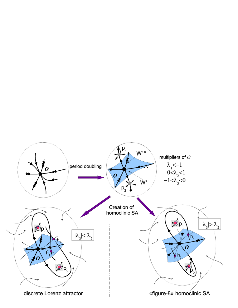
Figure 1: Main steps of creation of a homoclinic strange attractor: a discrete Lorenz attractor (below left), a “figure-eight” pseudo-hyperbolic strange attractor (below right).

In Fig. 1 this scenario is illustrated for the case when the periodic attractor $O$ is an asymptotically stable fixed fixed point; then this point loses stability via period doubling bifurcation, and a period 2 attractor appears so that the point $O$ becomes a saddle $O$ with $\dim W^{u}(O)=1$; and further the stable and unstable manifold of $O$ intersect (creating the “homoclinic attractor”). Note also that the period-2 attractor must lose stability. In the case when the point $O$ has multipliers $\lambda_{i}$ with that $\lambda_{1}<-1$, $0<\lambda_{2}<1,-1<\lambda_{3}<0$, $|\lambda_{3}|<\lambda_{2}$ and $|\lambda_{1}\lambda_{2}|>1$ the configuration of $W^{u}(O)$ is quite similar to those for the classical Lorenz attractor.

This scenario provides us with examples of truly high-dimensional (i.e. not two-dimensional) robust chaotic behavior which, as we sure, must occur in various applications. In the present paper we show that discrete Lorenz attractors can exist in Poincaré map of a nonholonomic model of Celtic stone, see also [16, 17].

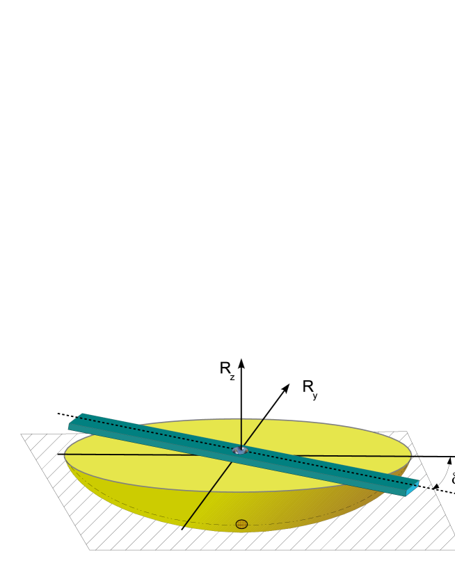
Figure 2: The sample of Celtic stone. The main body (of form of elliptic paraboloid) is symmetric with respect to the vertical axis $R_{z}$, the geometric horizontal axes are $R_{x}$ and $R_{h}$. The dynamical asymmetry is achieved due to a massive bar kept on the top of stone, which can be rotated by an angle $\delta$ with respect to the axis $R_{x}$. If $0<\delta<\pi/2$, the clockwise rotation of this stone is stable, whereas, the counterclockwise rotation is unstable.

Recall that, in the rigid body dynamics, the Celtic stone is a top (usually, of symmetric form which remains a boat, see Fig. 2) whose one of the principal inertial axes is vertical and other two axes are horizontal and they are rotated by some angle with respect to the geometrical axes. A nonholonomic model of Celtic stone is a mathematical model provided that both the stone and the plane are absolutely rigid and rough, i.e. the stone moves along the plane without slipping and, moreover, the friction force has zero moment. This means that the full energy is conserved which is a certain disadvantage of the model. However, it is well known that the nonholonomic model allows one to explain the main phenomenon of the Celtic stone dynamics – the nature of reverse, i.e., rotational asymmetry, which results in the fact that the stone can rotate freely in one direction (e.g. clockwise) but “does not want” to rotate in the opposite direction (counterclockwise). In the latter case it performs several rotations due to inertia, then stops rotating and starts oscillating, after that it changes the direction of rotation and finally continues rotating freely (clockwise).

A mathematical explanation of this phenomenon seems now simple enough. The fact is that, like most of the well-known nonholonomic mechanical models, the Celtic stone model is described by a reversible system, i.e., a system that is invariant with respect to the coordinate and time change of the form $X\to{\cal R}\;X,\;\;t\to-t$, where ${\cal R}$ is an involution, i.e. a specific diffeomorphism of the phase space such that ${\cal R}^{2}=Id$. However, in the case of Celtic stone, this system is, in general, neither conservative nor integrable, although it possesses two independent integrals (see formula (2.4)). Because of this, the system can possess, on the common level set of the integrals, asymptotic stable and completely unstable solutions, stationary (equilibria), periodic (limit cycles) solutions etc., ${\cal R}$-symmetric with respect to each other. Then, for example, a stable equilibrium corresponds to a stable vertical rotation of the stone, and an unstable equilibrium symmetric with respect to it corresponds to an unstable rotation in the opposite direction. Such an explanation of the reverse in the Celtic stone dynamics was given in a series of papers: by I.S. Astapov [18], A.V. Karapetyan [19], A.P. Markeev [20] and others (further references can be found in [21]).

Nevertheless, the motion of the Celtic stone is still regarded in mechanics as one of the most complicated and poorly studied types of rigid body motion. Moreover, this is one of the few types of motion in which chaotic dynamics was observed [22, 23, 24, 26].

The paper is organized as follows. Section 2 contains necessary facts related to a nonholonomic model of Celtic stone under consideration. Section 3 is the main part of the paper. In this section we consider the nonholonomic model of Celtic stone with parameters (3.1) and show (mostly numerically) that a discrete Lorenz attractor exists in this model. We study this problem using a research strategy (Section 3.2) based on fundamental facts from the theory of Lorenz-like attractors (see Section 3.1). Main results are formulated and discussed in Section 3.3.

2 The nonholonomic model of Celtic stone.

We study the dynamics of a rigid body moving on a plane without slipping. This means that we consider a nonholonomic model of motion in which the contact point of the body has zero velocity, i.e. we have

$${\mbox{{\bf{\em v}}}}+\boldsymbol{\omega}\times\mbox{{\bf{\em r}}}=0$$ (2.1)

where r is the radius vector from the center of mass $C$ to the contact point, v is the velocity of $C$ and $\boldsymbol{\omega}$ is the angular velocity of the body. As usual, the coordinates of all vectors are defined in some coordinates rigidly attached to the body. Then the equations of motion can be written in the form [28]

$$\begin{array}[]{l}\dot{\mbox{{\bf{\em M}}}}=\mbox{{\bf{\em M}}}\times\boldsymbol{\omega}+m\dot{\mbox{{\bf{\em r}}}}\times(\boldsymbol{\omega}\times\mbox{{\bf{\em r}}})+m{\mbox{g}}\mbox{{\bf{\em r}}}\times\boldsymbol{\gamma},\\ \dot{\boldsymbol{\gamma}}=\boldsymbol{\gamma}\times\boldsymbol{\omega},\end{array}$$ (2.2)

where

$$\mbox{{\bf{\em M}}}=\mbox{{\bf{\em I}}}\;\boldsymbol{\omega}+m{\mbox{{\bf{\em r}}}}\times(\boldsymbol{\omega}\times\mbox{{\bf{\em r}}})$$ (2.3)

is the angular momentum of the body with respect to the contact point, $\boldsymbol{\gamma}$ is the unit vertical vector and $m{\mbox{g}}$ is the gravity force. The equation (2.2) admits two integrals

$${\cal H}=\frac{1}{2}({\mbox{{\bf{\em M}}}},\boldsymbol{\omega})-m{\mbox{g}}({\mbox{{\bf{\em r}}}},\boldsymbol{\gamma})\;\;\mbox{and}\;\;(\boldsymbol{\gamma},\boldsymbol{\gamma})=1,$$ (2.4)

the energy integral and the geometric integral, respectively.

We consider the Celtic stone whose surface $F(\mbox{{\bf{\em r}}})$ has the shape of the elliptic paraboloid

$$F(\mbox{{\bf{\em r}}})=\frac{1}{2}\left(\frac{r_{1}^{2}}{a_{1}}+\frac{r_{2}^{2}}{a_{2}}\right)-(r_{3}+h)=0,$$

where $a_{1}$ and $a_{2}$ are the principal radii of curvature at the paraboloid vertex $(0,0,-h)$ respectively, and the center of mass is the point $r_{1}=r_{2}=r_{3}=0$. Therefore, the vector r and $\boldsymbol{\gamma}$ are related by:

$$\begin{array}[]{l}\displaystyle r_{1}=-a_{1}\frac{\gamma_{1}}{\gamma_{3}},\;\;r_{2}=-a_{2}\frac{\gamma_{2}}{\gamma_{3}},\;\;r_{3}=-h+\frac{a_{1}\gamma_{1}^{2}+a_{2}\gamma_{2}^{2}}{2\gamma_{3}^{2}}.\end{array}$$ (2.5)

It is also assumed that one of the principal axes of inertia is vertical. One of the main features of Celtic stone is that two other principal axes of inertia are rotated about the geometrical axes by some angle $\delta$, where $0<\delta<\pi/2$. Accordingly, the inertia tensor takes the following form [23]:

$$\mbox{{\bf{\em I}}}\;=\;\left(\begin{array}[]{ccc}I_{1}\cos^{2}\delta+I_{2}\sin^{2}\delta&(I_{1}-I_{2})\cos\delta\sin\delta&0\\ (I_{1}-I_{2})\cos\delta\sin\delta&I_{1}\sin^{2}\delta+I_{2}\cos^{2}\delta&0\\ 0&0&I_{3}\end{array}\right)\;\;,$$ (2.6)

where $I_{1},I_{2}$ and $I_{3}$ are the principal moments of inertia of the stone. We express vectors r, $\dot{\mbox{{\bf{\em r}}}}$ and $\boldsymbol{\omega}$ by M and $\boldsymbol{\gamma}$ using relations (2.1), (2.3), (2.5) and (2.6). Then the system (2.2) can be represented in the standard form

$$(\dot{\mbox{{\bf{\em M}}}},\dot{\boldsymbol{\gamma}})=G(\mbox{{\bf{\em M}}},\boldsymbol{\gamma},\mu),$$ (2.7)

of six-dimensional system with respect to phase variables M and $\boldsymbol{\gamma}$. This system depends also on parameters $\mu$ characterizing the geometrical and physical properties of the stone. Note that on the common level set of the integrals (2.4) the system (2.2) defines the flow on a four-dimension manifold: ${\cal M}^{4}=\{(\mbox{{\bf{\em M}}},\boldsymbol{\gamma}):(\boldsymbol{\gamma},\boldsymbol{\gamma})=1,{\cal H}(\mbox{{\bf{\em M}}},\boldsymbol{\gamma})=\mbox{const}\},$ which is homeomorphic to ${\mathbb{S}^{3}\times\mathbb{S}^{3}}$.

2.1 The Andoyer-Deprit variables.

In numerical investigations of dynamics of Celtic stone we use the so-called Andoyer-Deprit variables $(L,H,G,g,l)$ defined by the formulas [28]

$$\begin{array}[]{l}\displaystyle M_{1}=\sqrt{G^{2}-L^{2}}\sin l,\;\;M_{2}=\sqrt{G^{2}-L^{2}}\cos l,\;\;M_{3}=L,\\ \displaystyle\gamma_{1}=\left(\frac{H}{G}\sqrt{1-\frac{L^{2}}{G^{2}}}+\frac{L}{G}\sqrt{1-\frac{H^{2}}{G^{2}}}\cos g\right)\sin l+\sqrt{1-\frac{H^{2}}{G^{2}}}\sin g\cos l\\ \displaystyle\gamma_{2}=\left(\frac{H}{G}\sqrt{1-\frac{L^{2}}{G^{2}}}+\frac{L}{G}\sqrt{1-\frac{H^{2}}{G^{2}}}\cos g\right)\cos l-\sqrt{1-\frac{H^{2}}{G^{2}}}\sin g\sin l\\ \displaystyle\gamma_{3}=\frac{HL}{G^{2}}-\sqrt{1-\frac{L^{2}}{G^{2}}}\sqrt{1-\frac{H^{2}}{G^{2}}}\cos g\end{array}$$ (2.8)

By definition (see, e.g., [28]),

$$H=(\mbox{{\bf{\em M}}},\boldsymbol{\gamma})=M_{1}\gamma_{1}+M_{2}\gamma_{2}+M_{3}\gamma_{3}.$$ (2.9)

On the common level set of two integrals (2.4), the system (2.7) represents the four-dimensional flow ${\cal G}_{E}$. Note that the new coordinates $L,H,G,g$ and $l$ are chosen in such a way that the condition $(\boldsymbol{\gamma},\boldsymbol{\gamma})=1$ holds automatically. Thus, the formulae (2.8) specify a one-to-one correspondence between the coordinates $\{(\mbox{{\bf{\em M}}},\boldsymbol{\gamma}):\boldsymbol{\gamma}^{2}=1\}$ and $(L,H,G,g,l)$ everywhere except for the planes ${L}/{G}=\pm 1$ and ${H}/{G}=\pm 1$ (for which the coordinate $l$ and, respectively, $g$ are not defined).

Further, we will investigate the systems on the four-dimensional energy levels
${\cal H}(L,G,H,l,g)=E$. In this case the planes $g=g_{0}=\mbox{const}$ (for appropriate $g_{0}$) can be considered as cross-sections for orbits of the corresponding four-dimensional flow ${\cal G}_{E}$. Thus, we can also study the dynamics of the three-dimensional Poincaré map [22, 23]:

$$\bar{x}={\cal F}_{g_{0}}(x),\;\;x=\left(l,\frac{L}{G},\frac{H}{G}\right),$$ (2.10)

which is defined in the domain $0\leq l<2\pi,-1<\frac{L}{G}<1,-1<\frac{H}{G}<1$.

2.2 Symmetries in the Celtic stone model.

The system (2.7) possesses a number of interesting and useful symmetries described by the following lemma.

Lemma 1

[23] In the case under consideration, the system (2.7) is symmetric with respect to the coordinate changes:

$$(a)\qquad{\cal S}_{1}:\;\omega\to-(-\omega_{1},-\omega_{2},\omega_{3})\;\;,\;\;\gamma\to(-\gamma_{1},-\gamma_{2},\gamma_{3})\\$$ (2.11)

and is reversible with respect to the following involutions:

$$\begin{array}[]{l}(b)\qquad{\cal I}_{1}:\;\omega\to-\omega,\;\;,\;\;\gamma\to\gamma,\;\;,\;\;t\to-t\\ (c)\qquad{\cal I}_{2}:\;\omega\to(\omega_{1},\omega_{2},-\omega_{3})\;\;,\;\;\gamma\to(-\gamma_{1},-\gamma_{2},\gamma_{3}),\;\;t\to-t\end{array}$$ (2.12)

Note that these symmetries and involutions are also preserved for the Andoyer-Deprit coordinates. However, they cannot always be linear in this case. But for the Poincaré map (2.10) with the crosssection $g=0$, which we denote as ${\cal F}_{0}$, the symmetries (2.12) remain linear.

Lemma 2

[23] The map ${\cal F}_{0}$ is invariant under the following transformations:

$$\begin{array}[]{l}\vskip 3.0pt plus 1.0pt minus 1.0pt\displaystyle(a)\qquad\;\;\tilde{\cal S}_{1}:\;\;l\to l+\pi,\;\;\frac{L}{G}\to\frac{L}{G},\;\;\frac{H}{G}\to\frac{H}{G},\\ \vskip 3.0pt plus 1.0pt minus 1.0pt\displaystyle(b)\;\;\tilde{\cal I}_{1}:\;l\to l+\pi,\;\;\frac{L}{G}\to-\frac{L}{G},\;\;\frac{H}{G}\to-\frac{H}{G},\;\;{\cal F}_{0}\to{\cal F}_{0}^{-1}\\ \displaystyle(c)\;\;\tilde{\cal I}_{2}=\tilde{\cal I}_{1}\tilde{\cal S}_{1}:\;l\to l,\;\;\frac{L}{G}\to-\frac{L}{G},\;\;\frac{H}{G}\to-\frac{H}{G},\;\;{\cal F}_{0}\to{\cal F}_{0}^{-1}\end{array}$$ (2.13)

Corollary 1

Let $L^{*}$ be an orbit of ${\cal F}_{0}$. Then $\tilde{S}_{1}(L^{*})$, $\tilde{\cal I}_{1}(L^{*})$ and $\tilde{\cal I}_{2}(L^{*})$ are also orbits of ${\cal F}_{0}$. Moreover, the orbits $L^{*}$ and $\tilde{S}_{1}(L^{*})$, as well as $\tilde{\cal I}_{1}(L^{*})$ and $\tilde{\cal I}_{2}(L^{*})$, are symmetric with respect to each other. The orbits $L^{*}$ and $\tilde{S}_{1}(L^{*})$ are both in involution with the orbits $\tilde{\cal I}_{1}(L^{*})$ and $\tilde{\cal I}_{2}(L^{*})$.

3 On discrete Lorenz attractors in Celtic stone dynamics.

In this section we consider the nonholonomic model of Celtic stone whose physical parameters are as follows:

$$I_{1}=2,I_{2}=6,I_{3}=7,m=1,{\rm g}=100,a_{1}=9,a_{2}=4,h=1.$$ (3.1)

We also take $\delta=0.485$.

Note that the Celtic stone model with the parameters (3.1) was considered in [25] in which a strange attractor was found, with $E=770,\delta=0.405$. This strange attractor is quite similar to the attractor in Fig. 7(f). Since analogous attractors are known to exist in three-dimensional Hénon maps [13, 12] near the boundaries of destruction of discrete Lorenz attractors, the question naturally arises whether a discrete Lorenz attractor exists for close values of the parameters $E$ and $\delta$. The answer is positive and we give below a short review of results obtained.

Before description of main results (Sections 3.2 and 3.3)we make some remarks and recall necessary definitions.

3.1 On pseudo-hyperbolic Lorenz-like attractors.

First of all we give the definition of pseudo-hyperbolicity for diffeomorphisms, which is, in fact, a reformulation of the corresponding definition for flows from [5], see also [29].

Let $f$ be a $C^{r}$-diffeomorphism, $r\geq 1$ and let $Df$ be its linearization. An open bounded domain ${\cal D}\subset\mathbb{R}^{n}$ is absorbing for $f$ if $f(\overline{{\cal D}})\subset{\cal D}$.

Definition 1

The diffeomorphism $f$ is called pseudo-hyperbolic on $D$ if the following conditions hold.

• For each point of $D$ there exist two transversal subspaces $N_{1}$ and $N_{2}$ continuously depending on the point ($\dim N_{1}=k\geq 1,\dim N_{2}=n-k$) which are invariant with respect to $Df$:

  $$Df(N_{1}(x))=N_{1}(f(x)),\;\;Df(N_{2}(x))=N_{2}(f(x)).$$

  and for each orbit $L:\{x_{i}\;|\;x_{i+1}=f(x_{i}),\;i=0,1,...;x_{0}\in D\}$ the maximal Lyapunov exponent corresponding to the subspace $N_{1}$ is strictly smaller than the minimal Lyapunov exponent corresponding to the subspace $N_{2}$, i.e., the following inequality holds:

  $$\begin{array}[]{l}\displaystyle\lim\limits_{n\to\infty}\sup\frac{1}{n}\;\ln\;(\!\!\sup\limits_{\begin{array}[]{c}u\in N_{1}(x_{0})\\ \|u\|=1\end{array}}\!\!\|D^{n}f(x_{0})u\|)<\\ \qquad\qquad\qquad\displaystyle<\;\lim\limits_{n\to\infty}\inf\frac{1}{n}\;\ln\;(\!\!\inf\limits_{\begin{array}[]{c}v\in N_{2}(x_{0})\\ \|v\|=1\end{array}}\!\!\|D^{n}f(x_{0})v\|).\end{array}$$ (3.2)

• The restriction of $f$ to $N_{1}$ is contracting, i.e., there exist constants $\lambda>0$ and $C_{1}>0$ such that

  $$\|D^{n}f(N_{1})\|\leq C_{1}e^{-\lambda n}.$$ (3.3)

• The restriction of $f$ to $N_{2}$ expands volumes exponentially, i.e., there exist such constants $\sigma>0$ and $C_{2}>0$ such that

  $$|\det D^{n}f(N_{2})|\geq C_{2}e^{\sigma n}.$$ (3.4)

The following property immediately follows from this definition:

• All the orbits in ${\cal D}$ are unstable: each orbit has positive maximal Lyapunov exponent

  $$\Lambda_{max}(x)=\lim\limits_{n\to\infty}\sup\frac{1}{n}\;\ln\;\|D^{n}f(x)\|>0$$

Note that the pseudo-hyperbolicity conditions require the expansion of only $(n-k)$-dimensional volumes by the restriction of the diffeomorphism to $N_{2}$, which makes these conditions different from those for uniform hyperbolicity, where the following condition must hold: $\|D^{-n}f(N_{2})\|<Ce^{-\sigma n}$, i.e., the uniform expansion should be along all directions in $N_{2}$. Nevertheless, it is possible to establish the following fact in a standard way [30, 6].

• The pseudo-hyperbolicity conditions are not violated under small $C^{r}$-perturbations of the system. Moreover, the spaces $N_{1}$ and $N_{2}$ change continuously.

These two conditions imply that if the diffeomorphism $f$ has an attractor in ${\cal D}$, then this attractor is strange and does not contain stable periodic orbits, which also do not appear under small perturbations. In other words, pseudo-hyperbolic attractors are genuine strange attractor. The discrete Lorenz attractors form a certain subclass of the class of pseudo-hyperbolic attractors.

Note that the dynamical properties of the geometric Lorenz model [3] under small time-periodic perturbations were investigated in [5]. It was also shown that the properties of pseudo-hyperbolicity and chain transitiveness of a non perturbed Lorenz attractor hold for a periodically perturbed attractor as well. Thus, the Poincaré map also possesses here a pseudo-hyperbolic attractor $A$, which appears to be a basic example of a discrete Lorenz attractor. Note that the saddle equilibrium of the Lorenz attractor corresponds, after perturbations, to the saddle type fixed point of the corresponding Poincaré map.

The same conclusions can also be drawn without assuming that the map under consideration is a Poincaré map of a system periodic in time and close to an autonomous one. For this general case the corresponding definition of a discrete Lorenz attractor was given in [12]. Formally, this definition requires to satisfy main conditions which hold for the Poincaré map of periodically perturbed Lorenz attractor, including the geometrical analogy and the spectrum of Lyapunov exponents due to the Definition 1. Thus, for numerical study of a discrete Lorenz attractor, we need to check the required geometrical analogy and that fact that the numerical Lyapunov exponents $\Lambda_{1},\Lambda_{2},\Lambda_{3}$ satisfy conditions $\Lambda_{3}<\min\{\Lambda_{1},\Lambda_{2}\}$, $\Lambda_{3}<0$ and $\Lambda_{1}+\Lambda_{2}>0$ (some analogs of conditions (3.2), (3.3) and (3.4), respectively).

In Section 3.2 we describe the corresponding research strategy.The obtained results are collected in Section 3.3.

3.2 A strategy of qualitative and numerical study of discrete Lorenz attractors on example of the family ${\cal F}_{0E}$.

When studying dynamics and bifurcations in the family ${\cal F}_{0E}$ of the Poincaré map ${\cal F}_{0E}$ (2.10) for appropriate values of $E$ (with fixed $\delta=0.485$), we will act by employing the following strategy which, in fact, is justified by Definition 1 and its corollaries $1^{*}$ and $2^{*}$.

• Verify the geometrical similarity of our attractor $A_{E^{*}}$ found in the Celtic stone model to the Lorenz attractor. Here the strange attractor which was found for $E=E^{*}=752$ is examined.

In particular, this similarity manifests itself in the fact that our three-dimensional map ${\cal F}_{0E^{*}}$ possesses the following features: (i) it has a fixed saddle point $O^{*}$ belonging to the attractor $A_{E^{*}}$ with the multipliers of $\lambda_{1},\lambda_{2},\gamma$ such that $|\lambda_{2}|<|\lambda_{1}|<1<|\gamma|$, $\lambda_{1}>0,\lambda_{2}<0,\gamma<-1$ and $|\lambda_{1}\gamma|>1$; (ii) the manifolds $W^{u}(O)$ and $W^{s}(O)$ have nonempty intersection; (iii) the phase portraits look “similar”, see Fig. 3, and, moreover, the main bifurcations leading to appearance of the attractor are quite analogous to those in the Lorenz system, see item 4) below.

We mention that negative values of the multipliers $\lambda_{2}$ and $\gamma$ provide the Lorenz symmetry ($x\to x,y\to-y,z\to-z)$ of the homoclinic structure. Moreover, for the values of the parameter $E$ close to $E^{*}$, the manifold $W^{u}$ will intersect $W^{s}$ strictly from one side of the strong stable invariant manifold $W^{ss}(O)$, which is tangent to the eigendirection corresponding to the multiplier $\lambda_{2}$ of $O^{*}$, which provides the homoclinic configuration of the figure-eight-butterfly similar to the Lorenz attractor.

• Verify numerically the strangeness and pseudo-hyperbolicity of the attractor $A_{E^{*}}$.

At this stage we investigate the spectrum $\Lambda_{1},\Lambda_{2},\Lambda_{3}$ of the Lyapunov exponents of the map ${\cal F}_{0E^{*}}$ on the attractor $A^{*}$ and show that this spectrum, where $\Lambda_{1}>\Lambda_{2}>\Lambda_{3}$, satisfies the following conditions: (1) $\Lambda_{1}>0$; (2) $\Lambda_{1}+\Lambda_{2}+\Lambda_{3}<0$; (3) $\Lambda_{1}+\Lambda_{2}>0$. The conditions (1) and (2) imply that the attractor $A^{*}$ is strange and the condition (3) holds when the attractor is pseudo-hyperbolic (the map expands two-dimensional areas transversal to the strong contraction direction related to the exponent $\Lambda_{3}<0$).

• Plot numerically the dependence of the maximal exponent $\Lambda_{1}$ for some range of the parameter $E$ containing this value, $E=E^{*}$, for which the attractor $A_{E^{*}}$ exists, see Fig. 4.

At this stage we verify (only numerically) that our attractor is not a quasi-attractor, i.e., it does not contain stable periodic orbits of large periods, which do not appear under perturbations either. As is seen from Fig. 4, the graph resides in the domain $\Lambda_{1}>0$ and looks like a continuous function, whereas, if $A_{E^{*}}$ were a quasi-attractor, the “holes” would be observed on the plot containing the ranges of $\Lambda_{1}<0$ corresponding to “stability windows”.

• Investigate (mostly numerically) the main bifurcations starting at the stable fixed point and leading to the appearance of discrete Lorenz attractors (including $A_{E^{*}}$). We also trace the main stages of destruction of strange attractor.

In principle, this item may seem unnecessary but we suppose it to be the most interesting because here one can follow a certain “genetic” connection between the phenomena observed in flows with the Lorenz attractors (Lorenz model, Shimizu-Morioka model etc.) and those observed in the model of Celtic stone. Moreover, as the calculations show, our Poincaré map ${\cal F}_{0E}$ behaves like a “small perturbation of the time shift of the flow in the geometric Lorenz model” for corresponding values of $E$. Formally, this circumstance can be caused by the interesting fact that the middle Lyapunov exponent $\Lambda_{2}$ is very close to zero (for the flow case it is simply equal to zero): during calculations it demonstrates small oscillations in the range between $0.00007$ and $0.00015$, see [1] for a discussion of this topic. But what is really interesting is that the bifurcations leading to the appearance of strange attractor are here almost identical to those which accompany the birth of strange attractor in the Lorenz model [31], see. Fig. 5(b)–(f).

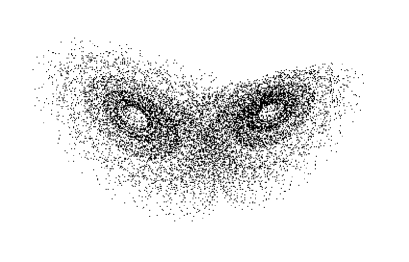
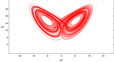
(a)	(b)

Figure 3: (a) a Lorenz-like attractor for $E=E^{*}=752$ in the Celtic stone model (about 10000 iterations of some initial point are shown); b) the projection of the Lorenz attractor from the Lorenz model onto the $(x,z)$ plane.

3.3 Results of the numerical study.

Below we show the results of numerical investigations performed according to items 1)–4) of the strategy.

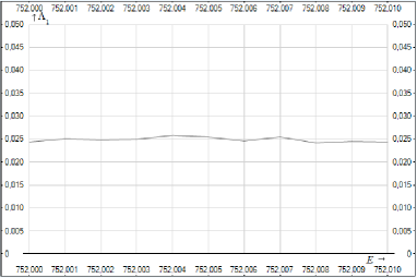
Figure 4: The plot of $\Lambda_{1}(E)$ in the range of $[752;752.01]$.

1) Fig. 3 shows (a) iterations of a single point of the attractor $A_{E^{*}}$ of the map $T_{E}$ for $E=E^{*}=752$ (for an appropriate angle of projection) and (b) the projection of orbits of the classical Lorenz attractor from the Lorenz model for $r=28$, $\sigma=10$, and $b=8/3$ onto the $(x,z)$ plane displayed for comparison.

The fixed saddle point $O^{*}$ with coordinates of $l=3.650;\;{L}/{G}=0.669;\;{H}/{G}=-0.384$ on the attractor $A_{E^{*}}$ has the multipliers $\lambda_{1}=0.996;\;\lambda_{2}=-0.664;\;\gamma=-1.312$. If one draws its unstable manifolds (“separatrices”), then, as expected, they will have “loops” (due to the existence of the homoclinic intersection), see Fig. 6(a), in contrast with the unstable separatrices of the Lorenz attractor in flows which appear to be sufficiently monotonous spirals.

2) For the attractor $A_{E^{*}}$ at $E=E^{*}=752$ the spectrum of the Lyapunov exponents was obtained as follows: $\Lambda_{1}=0.0248;\;\;\Lambda_{3}=-0.2445,\;\;0.00007<\Lambda_{2}<0.00015$.

Evidently, the conditions $\Lambda_{1}>0$, $\Lambda_{1}+\Lambda_{2}+\Lambda_{3}<0$ and $\Lambda_{1}+\Lambda_{2}>0$ hold here.

3) On the graph of Fig. 4 the dependence of the maximal Lyapunov exponent $\Lambda_{1}=\Lambda_{1}(E)$ on $E$ is shown for the range $[752;752.01]$ of the parameter $E$.

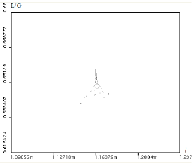
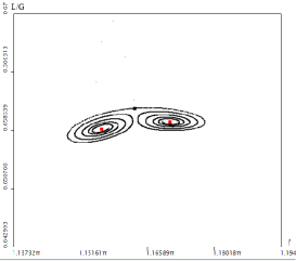
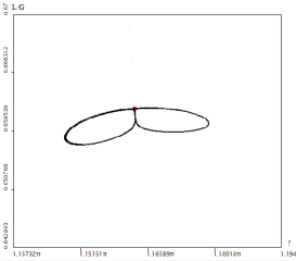
a) E=747	b) E=748.4	c) E=748.4395
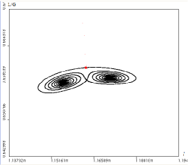
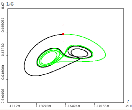
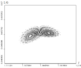
d) E = 748.5	e) E=750	f) E=750

Figure 5: The main stages of evolution of the Lorenz-like attractor in the map $T_{E}$. Figs. a) and f) show iterations of some starting point, and Figs. b)–g) show unstable manifolds of the fixed point $O$.

4) Fig. 5 illustrates the main stages of evolution of a discrete Lorenz attractor in the map ${\cal F}_{0E}$ for the parameter $E$ growing from $E=747$ to $E=E^{*}=750$.

Initially the attractor is a stable fixed point $O$, Fig. 5 a). Then, at $E=E_{1}=747.61$, it undergoes a period-doubling bifurcation, and the stable cycle $P=(p_{1},p_{2})$ of period two becomes an attractor, Fig. 5 b). At $E=E_{2}=748.4395$ the “homoclinic figure-eight-butterfly” of the unstable manifolds (separatrices) of the saddle $O$ is created, Fig. 5 c), which then gives rise to a saddle-type closed invariant curve $L=(L_{1},L_{2})$ of period two (where ${\cal F}_{0E}(L_{1})=L_{2},{\cal F}_{0E}(L_{2})=L_{1}$), the curves $L_{1}$ and $L_{2}$ surround the point $p_{1}$ and $p_{2}$, respectively. At the same time, the unstable separatrices of $O$ are rebuilt and now, for $E_{2}<E<E_{3}$, the left (right) one is coiled around the right (left) point of the cycle $P$, Fig. 5 d). Moreover, together with the closed period-$2$ invariant curve $L$, an invariant limit set $\Omega$ is born here, [31], which is not attracting yet. As the numerical calculations show, for $E=E_{3}\sim 748.97$ the separatrices “lie” on the stable manifold of the curve $L$ and then leave it. Almost immediately after that, at $E=E_{4}\sim 748.98$, the period-$2$ cycle $P$ sharply loses stability under a subcritical torus-birth bifurcation: the closed invariant curve $L$ merges with the cycle $P$, after that the cycle becomes a saddle and the curve disappears. The value of $E=E_{4}$ is the bifurcation moment of the creation of strange attractor – the invariant set $\Omega$ becomes attracting. Even for the parameter values close to $E=E_{3}$ (and $E>E_{3}$) the separatrices start to unwind, see Fig. 5 e) and their configuration becomes similar to the Lorenzian one, which also applies to the phase portrait, see Fig. 5 f).

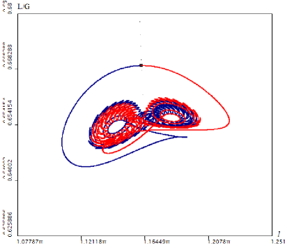
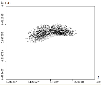
a)	b)

Figure 6:

Fig. 6 shows the behavior of (a) manifolds $W^{u}(O^{*})$ and b) iterations of the points on the attractor $A^{*}$ of map ${\cal F}_{0E^{*}}$ (here $E=E^{*}=752$). This attractor is studied in items 1)–3) above.

Fig. 7 shows some stages of destruction of the discrete Lorenz attractor, which is related to the appearance of resonant stable invariant curves , (b), (d) and (e), and the chaotic regimes (torus-chaos), (c) and (f). Note that for $E>790$ nothing remains of the discrete Lorenz attractor and the orbits run away from its neighborhood, tending to a new stable regime – the spiral attractor, observed in [24, 25].

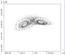
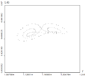
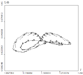
a) E=754	b) E=755	c) E=765
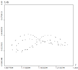
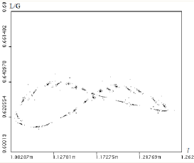
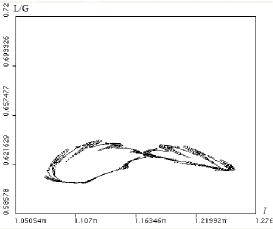
d) E= 770	e) E=775	f) E=780

Figure 7: Certain stages of destruction of the discrete Lorenz attractor: a) this is definitely a discrete Lorenz attractor; b), d) and e) various resonant invariant curves ; c) this attractor is very probably not of Lorenz type; f) a torus-chaos.

4 Conclusion.

The Lorenz attractors for flows play a special role in the theory of dynamical chaos. Until recently, these and hyperbolic attractors were the only ones which were classified as “genuine” strange attractors, which, in particular, do not allow the appearance of stable periodic orbits under small perturbations. After publication of the paper [6] by Turaev and Shilnikov the situation changed drastically. They not only provided an example of a wild hyperbolic spiral attractor that must be regarded as a genuine strange attractor but also introduced a new class of pseudo-hyperbolic attractors. Thus, a new trend related to the study of such strange attractors appeared in the theory of dynamical chaos.

Discrete Lorenz attractors should be considered as very interesting examples of such genuine attractors. However, unlike the flow Lorenz attractors, their mathematical theory has not been constructed yet. Although, the basic elements of this theory already exist, [6, 5, 1, 12], and “actively work”.

In particular, the example of a discrete Lorenz attractor found in this paper for the model of Celtic stone is, as we know, the first one for models from applications. However, we are sure that discrete Lorenz attractors exist in other models, one needs to make a more detailed search. Especially, since such attractors are not quite exotic, they could appear in dynamical systems (e.g. in three-dimensional maps) as a result of simple and universal bifurcation scenarios [13, 14].

Aknowledgements. The author are grateful to M. Malkin and D.Turaev for fruitful discussions and useful comments. This work has been partially supported by the Russian Scientific Foundation Grant 14-41-00044 and the RFBR grant 13-01-00589. Section 3 is carried out by the RSciF-grant (project No.14-12-00811).

References

- [1] Gonchenko S V, Ovsyannikov I I, Simó C and Turaev D, 2005, Three-dimensional Hénon-like maps and wild Lorenz-like attractors Int. J. Bif. And Chaos 15, 3493-3508.
- [2] Afraimovich V S, Bykov V V and Shilnikov L P, 1977, The origin and structure of the Lorenz attractor Sov. Phys. Dokl. 22, 253-255.
- [3] Afraimovich V S, Bykov V V and Shilnikov L P, 1982, On attracting structurally unstable limit sets of lorenz attractor type Trans. Mosc. Math. Soc. 44, 153-216.
- [4] Guckenheimer J and Williams R F, 1979, Structural stability of Lorenz attractors IHES Publ. Math. 50, 59-72.
- [5] Turaev D V and Shilnikov L P, 2008, Pseudo-hyperbolisity and the problem on periodic perturbations of Lorenz-like attractors Doklady Mathematics 77(1), 17-21.
- [6] Turaev D V and Shilnikov L P, 1998, An example of a wild strange attractor Sb. Math. 189, 291–314.
- [7] Newhouse S E, 1974, Diffeomorphisms with infinitely many sinks Topology 13, 9-18.
- [8] Aframovich V S and Shilnikov L P, 1983, Quasiattractors. in Nonlinear Dynamics and Turbulence, eds G.I.Barenblatt, G.Iooss, D.D.Joseph (Boston,Pitmen), 1983.
- [9] Benedicks M and Carleson L, 1991, The dynamics of the Henon map, Ann. Math. 133, 73-169.
- [10] Mora L and Viana M, 1993, Abundance of strange attractors Acta Math. 171(1), 1-71.
- [11] Ures R, 1995, On the Approximation of Hénon-like Attractors by Homoclinic Tangencies Ergod. Th. Dyn. Sys. 15, 1223–1229.
- [12] Gonchenko A S, Gonchenko S V, Ovsyannikov I I and Turaev D, 2013, Lorenz-Like Attractors in Three-Dimensional Hénon Maps, Math. Model. Nat. Phenom. 8(5), 80-92.
- [13] Gonchenko A S, Gonchenko S V and Shilnikov L P, 2012, Towards scenarios of chaos appearance in three-dimensional maps, Rus. Nonlinear Dynamics 8(1), 3-28.
- [14] Gonchenko A S, Gonchenko S V, Kazakov A O and Turaev D, 2014, Simple scenarios of oncet of chaos in three-dimensional maps, Int. J. Bif. And Chaos 24(8), 25 pages.
- [15] Borisov A V, Kazakov A O and Sataev I R, 2014, Phenomena of regular and chaotic dynamics in a nonholonomic model of Chaplygin top, Rus. Nonlinear Dynamics ??? (3), to appear.
- [16] Gonchenko A S, 2013, On Lorenz-like attractors in a model of Celtic stone, Vestnik UdGU mech., mat. 2(3), 3-11 (in Russian)
- [17] Gonchenko A S, Gonchenko S V, 2013, On existence of Lorenz-like attractors in a nonholonomic model of a Celtic stone, Rus. Nonlinear Dynamics 9(1), 77-89.
- [18] Astapov I S, 1980, On Rotation Stability of Celtic Stone, Vestnik Moskov. Univ. Ser. 1. Mat. Mekh. 2, 97–100. (Russian).
- [19] Karapetyan A V, 1981, On permanent rotations of heavy rigid body on the absolutely rough horizontal plane, J. Appl. Math. Mech. 45(5), 808–814.
- [20] Markeev A P, 1983, The Dynamics of a Rigid Body on an Absolutely Rough Plane, J. Appl. Math. Mech. 47(4), 473–478.
- [21] Markeev A P, 2011, Dynamics of a Body Touching a Rigid Surface, Moscow–Izhevsk: Regular and Chaotic Dynamics, Institute of Computer Science (Russian).
- [22] Borisov A V and Mamaev I S, 2002, Strange Attractors in the Rattleback Dynamics, Nonholonomic Dynamical Systems: Integrability, Chaos, Strange Attractors, Moscow–Izhevsk: Regular and Chaotic Dynamics, Institute of Computer Science, 296–326 (Russian).
- [23] Borisov A V and Mamaev I S, 2003, Strange Attractors in Rattleback Dynamics, 2003, Physics-Uspekhi 46(4), 393-403.
- [24] Gonchenko A S, Gonchenko S V and Kazakov A O, 2012, On new aspects of chaotic dynamics of “celtic stone”, Rus. Nonlinear Dynamics 8(3), 507-518.
- [25] Borisov A V, Jalnin A Yu, Kuznetsov S P, Sataev I R and Sedova J V, 2012, Dynamical phenomena occurring due to phase volume compression in nonholonomic model of the rattleback, Regular and Chaotic Dynamics 17(6), 512-532.
- [26] Gonchenko A S, Gonchenko S V and Kazakov A O., 2013, Richness of chaotic dynamics in nonholonomic models of Celtic stone, Regular and Chaotic Dynamics 15(5), 521-538.
- [27] Kazakov A O, 2013, Strange Attractors and Mixed Dynamics in the Unbalanced Rubber Ball on a Plane Problem, Regular and Chaotic Dynamics 18(5), 508-520.
- [28] Borisov A V and Mamaev I S, 2001, Dynamics of a Rigid Body, Moscow–Izhevsk: Regular and Chaotic Dynamics, Institute of Computer Science, (Russian).
- [29] Sataev E A, 2010, Stochastic properties of the singular hyperbolic attractors, Rus. Nonlinear dynamics 6(1), 187-206.
- [30] Anosov D V, 1967, Geodesic Flows on Closed Riemannian Manifolds of Negative Curvature, Proc. Steklov. Inst. Math. 90, 3–209.
- [31] Shilnikov L P, 1980, The Bifurcation Theory and the Lorenz Model, in: Bifurcation of the Cycle and Its Applications, Moscow: Mir, 317–335 (Russian).