Study of morphology and stellar content of the Galactic H ii  region IRAS 16148-5011

Abstract

An investigation of the IRAS 16148-5011 region - a cluster at a distance of 3.6 kpc - is presented here, carried out using multiwavelength data in near-infrared (NIR) from the 1.4 m Infrared Survey Facility telescope, mid-infrared (MIR) from the archival Spitzer GLIMPSE survey, far-infrared (FIR) from the Herschel archive, and low-frequency radio continuum observations at 1280 and 843 MHz from the Giant Metrewave Radio Telescope (GMRT) and Molonglo Survey archive, respectively. A combination of NIR and MIR data is used to identify 7 Class I and 133 Class II sources in the region. Spectral Energy Distribution (SED) analysis of selected sources reveals a 9.6 $~{}M_{\odot}$  high-mass source embedded in nebulosity. However, Lyman continuum luminosity calculation using radio emission - which shows a compact H ii  region - indicates the spectral type of the ionizing source to be earlier than B0-O9.5. Free-free emission SED modelling yields the electron density as 138 cm^-3, and thus the mass of the ionized hydrogen as $\sim$ 16.4 $~{}M_{\odot}$. Thermal dust emission modelling, using the FIR data from Herschel and performing modified blackbody fits, helped us construct the temperature and column density maps of the region, which show peak values of 30 K and 3.3$\times$10²² cm^-2, respectively. The column density maps reveal an A${}_{V}>$ 20 mag extinction associated with the nebular emission, and weak filamentary structures connecting dense clumps. The clump associated with this IRAS object is found to have dimensions of $\sim$ 1.1 pc$\times$0.8 pc, and a mass of 1023 $~{}M_{\odot}$.

1 Introduction

Most star formation activity is known to take place in clusters (Lada & Lada, 2003), and as such, observational studies of young embedded stellar cluster regions are imperative, because they serve as a template to further investigate various associated processes and their signatures. Due to the youth of such regions and the fact that their natal medium has still not been dispersed, these clusters can be used to scrutinize various theories related to star formation, stellar cluster dynamics, as well as stellar and cloud evolution. Of even more importance are the cluster regions which harbour high-mass stars, partly because such regions are few and far between, and more so as high-mass star formation is not very well understood (Zinnecker & Yorke, 2007).

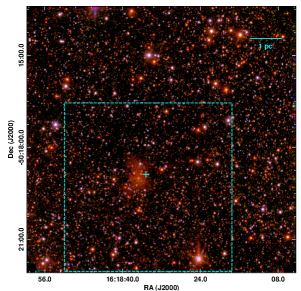
Figure 1: Colour composite image of the IRAS 16148-5011 region, made using the $K_{s}$ (red), $H$ (green), and $J$ (blue) band images. The area of analysis in this paper has been marked by the dashed rectangle. Plus symbol marks the IRAS catalogue position of IRAS 16148-5011. The scale bar shows 1 pc extent at a distance of 3.6 kpc.

IRAS 16148-5011 is an infrared nebula (Fig. 1) in the southern sky ($\alpha_{2000}=16^{h}18^{m}35.2^{s}$, $\delta_{2000}=-50^{o}18\arcmin 53\arcsec$) associated with which is an IR cluster found using the Two Micron All-Sky Survey (2MASS) data by Dutra et al. (2003). It is located at the Galactic plane ($l\sim 333.047^{o},b\sim+0.037^{o}$) and is in the vicinity of the well-known star-forming region RCW 106. Though other star-forming regions are present nearby, IRAS 16148-5011 appeared to be a relatively isolated region in past mappings (Karnik et al., 2001; Mookerjea et al., 2004). Kinematic distance estimates to this region vary from $\sim$ 3.3-11.9 kpc (near- and far-distance estimates; Molinari et al., 2008), and we adopt the distance of 3.6 kpc from Lumsden et al. (2013) (based on the spectrophotometric distance of a prominent source - “G333.0494$+$00.0324B”  in their nomenclature - associated with the central nebula) for our work. The compilation of Lumsden et al. (2013) also reveals other nearby regions at this distance, providing preliminary indications that this could be a part of larger complex. In the early analyses of Haynes, Caswell, & Simons (1979) (also see Chan, Henning, & Schreyer, 1996), radio continuum emission at 6 cm was detected, with peak in the neighbourhood ($\gtrsim$ 1′ , positional accuracy $\sim$ 30″ ) of this region, and it was predicted to be harbouring massive young stellar objects. The IRAS colour analysis by MacLeod et al. (1998) was also found to be consistent with that for an H ii  region, and Molinari et al. (2008) - using the IRAS “[25-12]”  colour value - have suggested that this region is among the younger IRAS detected regions. A high-mass stellar source was detected by Grave & Kumar (2009) with the help of spectral energy distribution (SED) fitting using NIR to millimeter data. Analyses of this region at 1.2 mm dust continuum emission and at molecular lines have revealed the presence of dense gas, with a large column density, as well as massive clumps. The total luminosity estimate ($\sim$ 4.4$\times$10⁴ L_⊙, by integrating IRAS flux densities) has also been found to be well in the regime of high-mass stellar objects (Beltrán et al., 2006; Fontani et al., 2005). Therefore, taking into account these characteristics, this region makes a good candidate to carry out an investigation for understanding the morphology and stellar population. However, since this is a possible H ii  region with an embedded cluster, multiwavelength observations are required to fully discern this region’s various constituents and how they relate to each other. In this paper, we have tried to accomplish this using deep NIR observations, archival MIR Spitzer data, archival FIR Herschel data, and low-frequency radio continuum observations.

In Section 2, we detail the various observations and the corresponding data analysis procedures, followed by an examination of the stellar population in the region in Section 3. The morphology of the region is discussed in Section 4. Discussion and conclusions are presented in Sections 5 and 6, respectively.

2 Observations and data reduction

2.1 Near-Infrared Observations

NIR photometric observations in $J$ (1.25 $\mu$m), $H$ (1.63 $\mu$m), and $K_{s}$ (2.14 $\mu$m) bands (centered on $\alpha_{2000}\sim 16^{h}18^{m}31^{s}$, $\delta_{2000}\sim-50^{o}17^{{}^{\prime}}32^{{}^{\prime\prime}}$) were carried out on 2004 July 29 using the 1.4 m Infrared Survey Facility (IRSF) telescope, South Africa. The observations were taken with the help of the Simultaneous InfraRed Imager for Unbiased Survey (SIRIUS) instrument, a three colour simultaneous camera mounted at the f/10 Cassegrain focus of the telescope. SIRIUS is equipped with three 1k$\times$1k HgCdTe arrays, each of which, with a pixel scale of 0.45″ , provide a field of view (FoV) of 7.8′ $\times$7.8′ . Further details can be obtained from Nagashima et al. (1999) and Nagayama et al. (2003). Five sets of frames, with each set containing observations at ten dithered positions (exposure time of 5 s at each dither position), were obtained (i.e. total exposure time = 5$\times$10$\times$5 s = 250 s, in each band). The sky conditions were photometric, with a seeing size of $\sim$ 1.35″ . In addition to the target field, a sky region ($\sim$ 10′  to the north of target region) and the standard star P9172 (Persson et al., 1998) were also observed.

Following a standard data reduction procedure, which involved bad pixel masking, dark subtraction, flat-field correction, sky subtraction, combining dithered frames, and astrometric calibration, point spread function (psf) photometry was carried out using the allstar algorithm of the daophot package in iraf. About 11-13 sources were used to construct the psf for each band. Finally the instrumental magnitudes were calibrated using the standard star P9172. The astrometric calibration rms obtained was $<$ 0.05″, and the median photometric error $<$ 0.05 mag. On comparing our catalogues with the 2MASS catalogues, sources with $K_{s}$ magnitude $\leq$ 9.5 were found to be saturated, and hence had their $J,H,$ and $K_{s}$ magnitudes replaced by the corresponding 2MASS magnitudes. The final NIR catalogue is used to identify the young stellar objects (YSOs) in the region. The area of study in this paper is about 5.5′$\times$5.5′  encompassing the nebular cloud region, centered on $\alpha_{2000}\sim 16^{h}18^{m}35^{s}$, $\delta_{2000}\sim-50^{o}19^{{}^{\prime}}18^{{}^{\prime\prime}}$.

Completeness limits were calculated for all three bands by carrying out artificial star experiments using the addstar package in iraf. A fixed number of stars were added in each 0.5 magnitude bin and analysis carried out to see how many stars are detected. The ratio of the number of detected stars to the number of added stars gives us the completeness fraction as a function of magnitude. The 90% completeness limit was thus calculated as 16.6, 15.8, and 15.5 for the $J,H,$ and $K_{s}$ bands, respectively.

2.2 Radio Continuum Observations

Radio continuum observations at 1280 MHz were obtained on 2012 November 09 using the Giant Metrewave Radio Telescope (GMRT) array. The GMRT array consists of 30 antennae arranged in an approximate Y-shaped configuration, with each antenna having a diameter of 45 m. This translates to a primary beam-size of 26.2′  at 1280 MHz. A central region of $\sim$1 km$\times$1 km contains 12 randomly distributed antennae, while the remaining 18 are along the three radial arms (6 along each arm) which extend upto $\sim$14 km. Details about the GMRT can be found in Swarup et al. (1991).

For our observations, the Very Large Array (VLA) phase and flux calibrators ‘1626-298’  and ‘3C286’ , respectively, were used. The total observation time (including the calibrators) was about 3.5 hrs, limited by the low declination of the source. Data reduction was carried out using the aips software. Initial steps involved flagging the bad data (carried out using a combination of ‘vplot-uvflg’  and ‘tvflg’  tasks) and calibration (carried out using ‘calib-getjy-clcal’ ). After a few iterations of flagging and calibration, the source data was ‘split’  from the whole, and was used for imaging using the task ‘imagr’ . A few rounds of (phase) self-calibration were also carried out using the task ‘calib’  to remove any ionospheric phase distortion effects. To check that the flux calibration was done correctly, the image of the flux calibrator was constructed, and its flux determined and checked against literature values. The final (target) source images were rescaled to take into account the system temperature corrections for the GMRT. These corrections are required as, at the Galactic plane, the large amount of radiation at meter wavelengths increases the effective temperature of the antennae. This was done as follows. Using the sky temperature map of Haslam et al. (1982) at 408 MHz, and the spectral index of -2.6 given therein, the temperature towards this region was obtained, i.e. $T_{frequency}=T_{408}\times(frequency/408\,{\rm MHz})^{-2.6}$, where $T_{408}$ is the temperature at 408 MHz and $T_{frequency}$ is the temperature at required $frequency$ (1280 MHz here). The images were subsequently rescaled by a factor given by $(T_{frequency}+T_{sys})/T_{sys}$, i.e. the ratio of temperature towards the target to that towards the flux calibrator. $T_{sys}$, the system temperature, was obtained from the GMRT manual.

In addition to the GMRT observations, we also obtained the archival first epoch Molongolo Galactic Plane Survey (MGPS) data at 843 MHz (Green et al., 1999). The MGPS observations were carried out using the Molonglo Observatory Synthesis Telescope (MOST) with a resolution of 43″ $\times$43″ cosec |Declination| . For our analysis purpose, we retrieved the original processed image for this region’s Galactic coordinates (resolution $\sim$ 55.84″$\times$43″ ) from the website. The radio images are used to obtain the physical parameters and examine the morphology of the ionized gas in the region (see Section 4.2).

2.3 Other Archival Data Sets

2.3.1 Spitzer mid-infrared observations

Archival MIR observations of this region, obtained using the Spitzer Space Telescope under the Galactic Legacy Infrared Midplane Survey Extraordinaire (GLIMPSE) program (Benjamin et al., 2003; Churchwell et al., 2009), were retrieved with the help of the InfraRed Science Archive (the Spring ’07 Archive more complete catalogue). GLIMPSE observations were taken using the InfraRed Array Camera (IRAC) in 3.6, 4.5, 5.8, and 8.0 $\mu$m bands. The final image cutouts (pixel scale of 0.6″ ) as well as the final catalogues were downloaded. While the images are further used to analyse features in the region, the photometric catalogue, in conjunction with the NIR catalogue (Section 2.1) was used to identify the YSOs in the region.

2.3.2 Herschel far-infrared observations

This region has been observed at FIR wavelengths, in the range 70-500 µm , using the instruments Photodetector Array Camera and Spectrometer (PACS; Poglitsch et al., 2010) and Spectral and Photometric Imaging Receiver (SPIRE; Griffin et al., 2010) on the 3.5 m Herschel Space Observatory (Pilbratt et al., 2010), as a part of the Proposal ID “KPOT_smolinar_1”  (Molinari et al., 2010). For our analyses, we obtained the PACS 70 µm  and 160 µm  level2_5 MADmap images (Cantalupo et al., 2010); and the SPIRE 250 µm , 350 µm , and 500 µm  level2_5 extended source (“extdPxW” ) map products using the Herschel Science Archive. The 70 µm, 160 µm , 250 µm , 350 µm , and 500 µm  images have pixel scales of 3.2″ , 6.4″ , 6″ , 10″ , and 14″ , respectively, with resolutions varying from $\sim$ 5.5″ –36″ . While the PACS image obtained had the surface brightness unit of Jy pixel^-1, the SPIRE images were in the units of MJy sr^-1. Detailed information about the data products is provided on the Herschel site. We use the FIR data to examine the physical conditions of the region.

3 Stellar Population in the region

3.1 Identification of YSOs

The NIR and MIR photometric catalogues from IRSF (Section 2.1) and GLIMPSE (Section 2.3.1), respectively, were cross-matched within 0.6″  matching radius and collated to obtain a combined photometric catalogue. Thereafter, the following set of steps were followed for the identification of the YSOs (similar to Mallick et al., 2013) :

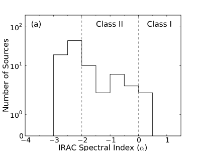
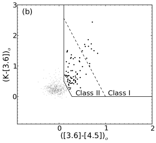
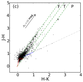
Figure 2: (a) Histogram of the IRAC spectral indices. The limits for Class I and Class II sources have been marked by dashed grey vertical lines. (b) NIR-MIR CCD using the procedure of Gutermuth et al. (2009). The regions of Class I and Class II sources have been labelled. The identified YSOs have been shown with black solid circles. (c) NIR CCD in CIT system. The red curve and the blue line show the dwarf locus (Bessell & Brett, 1988) and the CTTS locus (Meyer, Calvet, & Hillenbrand, 1997), respectively. The grey dot-dashed line is the extension of CTTS locus. Three parallel slanted dashed lines mark the reddening vectors, drawn using extinction laws from Cohen et al. (1981). Three separate regions, ‘F’ , ‘T’ , ‘P’  have been labelled on the plot. The source marked with a cross in ‘P’  region is a high-mass YSO (see text).

1. First, the YSOs were identified using their MIR magnitudes. The sources with detections in all four IRAC bands with errors $\leq$ 0.15 mag were used here. Using simple linear regression, the IRAC spectral index ($\alpha_{IRAC}=d\log(\lambda F_{\lambda})/d\log(\lambda)$; Lada, 1987) was calculated for each source (in the wavelength range 3.6-8.0 µm), followed by their classification into Class I and Class II categories using the limits from Chavarría et al. (2008) ($\alpha_{IRAC}>0$ for Class I, and $-2\leq\alpha_{IRAC}\leq 0$ for Class II; see Fig. 2).

2. All sources need not have detections at 5.8 and 8.0 $\mu$m, but might have good quality detections in NIR bands. To identify the YSOs from amongst such sources, we use a combination of $H,K_{s}$, 3.6 $\mu$m, and 4.5 $\mu$m bands following the procedure of Gutermuth et al. (2009). Again, only those sources whose 3.6 and 4.5 $\mu$m magnitude errors are $\leq$ 0.15 are used here. The YSOs were identified from their location in the dereddened - using the colour excess ratios from Flaherty et al. (2007) - “$K_{s}$-[3.6]”  versus “[3.6]-[4.5]”  colour-colour diagram (CCD), as is shown in Fig. 2.

3. Additional YSOs were identified using the $J-H/H-K$ CCD (Fig. 2) according to the following procedure. In Fig. 2, the red solid curve marks the dwarf locus from Bessell & Brett (1988) and the blue solid line marks the Classical T Tauri Stars (CTTS) locus from Meyer, Calvet, & Hillenbrand (1997). All the loci curves as well as sources’ colours were converted to CIT (California Institute of Technology) photometric system (using Carpenter, 2001) for this analysis. The slanted dashed lines are the reddening vectors, drawn using the reddening laws of Cohen et al. (1981) for the CIT photometric system. In this CCD, three separate regions have been marked, similar to Ojha et al. (2004a, b). The sources in ‘T’  and ‘P’  regions are taken to be Class II sources (Lada & Adams, 1992), as they exhibit IR-excess emission. In the ‘P’  region, since there could be a slight overlap between Herbig Ae/Be stars and Class II sources (Hillenbrand et al., 1992), we conservatively took only those sources which were above the CTTS locus extended into this region (similar to Mallick et al., 2014). It should be noted that sources in the ‘T’  region could also contain a few Class III sources with small IR-excess.

Finally, we merged the sources identified in each step. An overlapping source might have different identifications in different steps. Thus, in the final list, the class of a YSO was taken as that in which it was identified as first in the above order of steps. A total of 7 Class I and 133 Class II sources were obtained (for a FoV of $\sim$ 5.5′$\times$5.5′  encompassing the molecular cloud, as marked in Fig. 1) in the final YSO catalogue, which is given in Table 1.

3.2 Spectral Energy Distribution of YSOs

SED modelling was carried out for (a subset of) YSOs to get estimates of their physical parameters. The grid of YSO models from Robitaille et al. (2006) - implemented in the online SED fitting tool of Robitaille et al. (2007) - was used for this purpose. The basic model consists of a pre-main sequence (PMS) star surrounded by a flared accretion disk having a rotationally flattened envelope with cavities carved out by a bipolar outflow. A total of 200000 SED models are computed in a 14 dimensional parameter space (covering properties of the central source, the infalling envelope, and the disk), using the radiation transfer code of Whitney et al. (2003a, b). The online fitting tool attempts to fit the available SED models to the data, characterising each fitting by a $\chi^{2}$ parameter. The distance range and the interstellar visual extinction (A_V) are free parameters whose range has to be specified by the user. Accounting for the uncertainties, we adopted a large distance range of 3.4 to 3.8 kpc for our sources. From extinction calculations (see Section 4.1) we find that almost all non-YSO sources had A${}_{V}\leq$ 20 mag, and thus we specified the range of interstellar visual extinction A_V as 1-20 mag.

Since the number of SED models is very large, spanning a wide range of parameter space, the models fitting each source can only be constrained by increasing the number of data points used, and having data points to sufficiently cover the entire wavelength range of fitting. For this reason, we choose the sources with photometry in at least all four IRAC bands for SED modelling. However, in addition to those selected using this criterion, we also carried out SED analysis for the prominent sources associated with the central nebula (even though two of them lacked 8.0 µm  photometry). We note that photometry from Herschel images is not useful here as none of the YSOs have counterparts at those wavelengths, which in part is due to poor resolution.

For each source, the SED fitting tool - besides giving the best fit model - also gives a set of well fit models ranked by their $\chi^{2}$ values as a measure of their relative “goodness-of-fit”. Following a method similar to Robitaille et al. (2007), we consider only those models for further calculation which satisfied the following criterion :

$$\chi^{2}-\chi^{2}_{min}<3\ \rm{(per\ data\ point)}.$$ (1)

As elucidated in Robitaille et al. (2007), though this criterion is based on visual examination of SED plots and has no rigid mathematical backing, a stricter criterion might lead to over-interpretation. For each parameter, the weighted mean value and standard deviation were calculated using the models which satisfied Equation (1). The inverse of the respective $\chi^{2}$ was taken as the weight for each model (similar to Grave & Kumar, 2009). Table 2 gives our SED modelling results, listing the physical parameters : age of the central source (t_∗), mass of the central source, disk mass ($M_{disk}$), disk accretion rate ($\dot{M}_{disk}$), envelope mass ($M_{env}$), temperature of the central source ($T_{*}$), total system luminosity ($L_{total}$), interstellar visual extinction (A_V), and the $\chi^{2}_{min}$ per data point. Errors for some parameters tend to be large as we are dealing with a large parameter space while we have very few data points to constrain the number of models. If a source was simply fit better as a star with high interstellar extinction, it has not been included in the table. Thus finally, SED results are given for a total of 3 Class I sources, 24 Class II sources (including 2 central sources), and one extra central source.

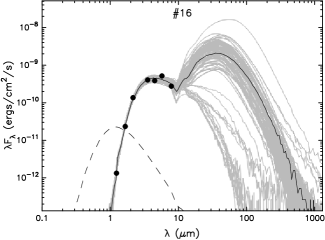
Figure 3: SED fitting using the online tool of Robitaille et al. (2007) for source #16 (a Class II source) in Table 2. The black dots mark the data points. The solid black curve is the best fitted model, while the grey curves denote the subsequent good fits for $\chi^{2}-\chi^{2}_{min}(per~{}data~{}point)<3$. The dashed curve is the photosphere (in the presence of interstellar extinction, but absence of circumstellar dust) of the central source for the best-fit model.

Even though the statistics for the YSOs (i.e. Class I and Class II sources) is not very significant, we can still use them to get an idea of the physical parameters of the stellar sources forming in this region. As can be seen from Table 2, there appears to be a considerable age dispersion, with the ages ranging from $\sim$ 0.05 Myr to 0.5 Myr for most of the sources. 5 YSOs even have ages $>$ 1 Myr. This is suggestive of ongoing star formation. All the YSOs analysed here yield masses $>$ 2 $~{}M_{\odot}$, and five of them $>$ 6 $~{}M_{\odot}$. One of the YSOs (#16) appears to be a high-mass star of $\sim$ 9.6 $~{}M_{\odot}$, and is embedded in the nebular emission associated with this region (see Section 4). The SED plot for this source is shown in Fig. 3. Grave & Kumar (2009) had also done SED analysis for what they mention as an embedded point source in this IR nebula with $JHK$ and four IRAC bands. Since among the possible embedded sources in the central part of this IR nebula, only this source (#16) had all 7 magnitudes, most likely their ‘16148-5011mms2near’  refers to this source itself. Grave & Kumar (2009) calculated the age and mass of this source as 4.2$\pm$0.3 ($\log t_{*}$) and 11$\pm$1 $~{}M_{\odot}$, respectively. Though the mass estimate appears consistent (within error limits) with our results, their age estimate is much lower. It is probable that this could be because they use different distance estimates and 1.2 mm fluxes from literature. This source is also classified as a YSO by Lumsden et al. (2013, called “G333.0494$+$00.0324B” ). Another source (#28) associated with the nebula appears to be a high-mass stellar object, with age $>$ 1 Myr, though it is not classified as a YSO in our analysis.

It should be noted that the SED results are only representative of the actual values, as an empirically consistent fit might not be the correct fit. A deliberate sampling bias of the huge parameter space, to reduce computational time, could give rise to pseudotrends in the results. The results are also contingent upon the validity of assumed evolutionary tracks from literature. Most importantly, the models are for individual sources, and could be misleading in cases of stellar multiplicity. The caveats are dealt in detail in Robitaille (2008).

3.3 Luminosity Function

The slope of the $K_{s}$-band luminosity function (KLF) can serve as an indicator of the age of a stellar cluster (Zinnecker, McCaughrean, & Wilking, 1993; Lada & Lada, 1995; Vig et al., 2014). If we were to assume that the mass function and the mass-luminosity relation for a (coeval) stellar cluster are power laws, i.e. they are of the form $dN(\log m_{*})\propto m_{*}^{-\gamma}d\log m_{*}$ and $L_{K}\propto m_{*}^{B}$, then it can be shown that the slope of the KLF will be of the form :

$$\alpha=\gamma/2.5B$$ (2)

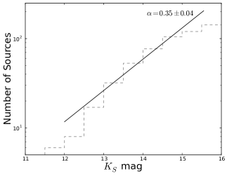
Figure 4: The grey dashed histogram shows the cumulative KLF for the YSOs. The black straight line is the fit in [12,15.5] mag range, whose slope is given by $\alpha$.

(Lada, Young, & Greene, 1993; Megeath, 1996). First of all, we try to estimate the KLF slope. We only consider the YSOs here, as opposed to all the observed sources, as they will be much less affected by any field star contamination. Our K-band 100% completeness limit is upto 14 mag, and thus completeness correction was implemented in the (0.5 mag sized) bins after this limit. Thereafter, the (cumulative) KLF of the YSOs was constructed, and is shown in Fig. 4. The fit to the histogram is also shown, and its slope ($d\log N/dm_{K}$) in [12,15.5] mag range is calculated to be ($\alpha=$) 0.35$\pm$0.04 (the slope will be same for cumulative and differential KLFs here, see Lada, Young, & Greene, 1993). As for the slope of mass-luminosity relation, if we adopt the value of $B=2$ (which can be shown to be the approximate value for O-F main sequence stars; Lada, Young, & Greene 1993), then the mass function slope comes out to be ($\gamma=$)1.75$\pm$0.20 (a value slightly steeper than the Salpeter slope of 1.35).

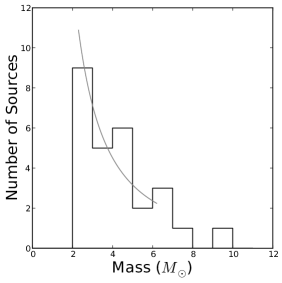
Figure 5: Histogram of stellar masses obtained from the SED fitting (Table 2). The grey curve shows the power law fit in the intermediate mass range.

Alternatively, we could get an estimate of the mass function slope using the SED fitting results. Since most of our sources are of intermediate mass in 2-6 $~{}M_{\odot}$  range (see Table 2), we consider only this range to estimate the slope $\gamma$. Fig. 5 shows the mass histogram (for the YSOs). Assuming that the star formation is strictly coeval, the mass function slope is given by $\gamma=-(d\log N/d\log m_{*})$ (Massey, 1998), and thus we calculate $\gamma\sim 1.59\pm 0.70$ for our case. The grey curve in Fig. 5 shows the fitted function for 2-6 $~{}M_{\odot}$. This is consistent with $\gamma$ obtained above. The major source of uncertainty here is the sparse statistics, and thus possible incompleteness in the mass bins.

A similar set of values (both $\alpha$ and $\gamma$) was found by Balog et al. (2004) for the 1 Myr old NGC 7538 cluster (distance $\sim$ 2.65 kpc; Mallick et al., 2014). $\alpha$ also appears consistent with that derived for the Orion molecular clouds ($\sim$ 0.37-0.38, age $\sim$ 1 Myr; Lada & Lada, 1995; Lada et al., 1991). However, other embedded clusters in literature, such as the NGC 1893 cluster ($\sim$ 0.34$\pm$0.07, distance $\sim$ 3.25 kpc; Sharma et al., 2007), the Tr 14-16 clusters in Carina nebula ($\sim$ 0.30-0.37, distance $\sim$ 2.5 kpc; Sanchawala et al., 2007), and the IRAS 06055+2039 cluster ($\sim$ 0.43$\pm$0.09, distance $\sim$ 2.6 kpc; Tej et al., 2006) do exhibit slightly larger cluster ages, upto $\sim$ 4 Myr. Hence it appears that 1 Myr should be the lower age limit of the cluster.

3.4 Mass Spectrum

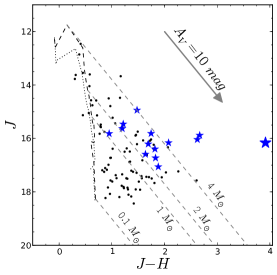
Figure 6: $J$/$J-H$ colour-magnitude diagram for the YSOs with at least $J$ and $H$ band detections. The dashed and dotted black curves plot the 1 Myr and 2 Myr PMS isochrones, respectively, from Siess, Dufour, & Forestini (2000). The reddening vectors (parallel grey dashed lines) for the 1 Myr isochrone are drawn at 0.1, 1, 2, and 4 $~{}M_{\odot}$. The blue star symbols are the sources for which SED analysis was done.

In addition to the SED, we also use the $J/J-H$ colour-magnitude diagram (CMD) to get an estimate of the mass range of the YSOs. We avoid using a CMD involving the $K$-band magnitude as this band is the most affected by the NIR excess flux arising from circumstellar material, which in turn can lead to brightening, and thus erroneous mass estimate, of the sources. Fig. 6 shows the $J/J-H$ CMD for the YSOs with at least $J$ and $H$ band detections. The 1 Myr PMS isochrone, along with the 2 Myr isochrone for reference, from Siess, Dufour, & Forestini (2000) has been shown on the image. For the 1 Myr PMS isochrone, reddening vectors are shown for 0.1, 1, 2, and 4 $~{}M_{\odot}$ . As can be seen, all but one of the YSOs for which the SED analysis has been done (marked with blue stars) lie in the mass range $\ga$ 2 $~{}M_{\odot}$ , matching well with our SED results. In general, the sources lie in the mass range $\sim$ 0.1-4 $~{}M_{\odot}$, or, put differently, the observations probe stellar objects upto the 0.1 $~{}M_{\odot}$  limit. The (blue star) source at the far-right end of the diagram is the 9.6 $~{}M_{\odot}$  high-mass source from SED analysis. The wide variation in the colours of YSOs is probably an indication of variable extinction as well as different evolutionary stages of the sources. Major causes of uncertainty here are : uncertainty in distance estimate which is used to obtain the apparent magnitude (for the isochrones), and unresolved (especially since the source distance of $\sim$  3.6 kpc is much larger than most of the previously studied clusters) binarity. Additionally, it should be kept in mind that, in general, a particular PMS model will introduce its own systematic error.

4 Morphology of the Region

4.1 Cluster Analysis and Extinction mapping

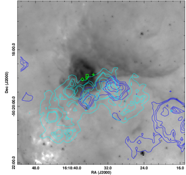
Figure 7: Spitzer 8.0 $\mu$m image of the region with overlaid surface density contours (at 5, 5.75, 6, 7, 7.5, and 8 YSOs pc^-2) in cyan, and visual extinction contours (at A_V = 4, 4.5, 5, 6, and 6.5 mag) in blue. Green plus symbol marks the IRAS catalogue position of IRAS 16148-5011, green cross the high-mass source (#16 from Table 2), while the diamond and box symbols mark the millimeter and MSX peaks, respectively, from Molinari et al. (2008).

Fig. 7 shows the Spitzer 8.0 $\mu$m image with overlaid surface density contours (in cyan) as well as visual extinction contours (in blue). The high-mass source in this region (see Section 3.2), as well as the millimeter (mm) and MSX peaks from Molinari et al. (2008, 16148-5011 MM 1 and 16148-5011 A from their Tables 2 and 3, respectively) have also been marked on the image. The marked mm peak is almost coincident with the (mm) peak from Beltrán et al. (2006, 16148-5011 Clump 2 from their Table 2). The surface density and extinction contours were calculated as follows. The surface density analysis was carried out using the nearest-neighbour (NN) method (Casertano & Hut, 1985) to discern the YSO clusterings in the region. We chose 20 NN, similar to Schmeja, Kumar, & Ferreira (2008); Schmeja (2011); Mallick et al. (2013). The extinction in the region was estimated by constructing the extinction map with the help of the NIR photometric data. We use the NIR CCD (see Fig. 2) for this purpose. In this NIR CCD, the ‘F’  region mostly contains the main-sequence field sources along with a few probable Class III sources. Since these are sources which have almost lost their circumstellar material, any extinction they exhibit will come from interstellar - rather than circumstellar - material. The sources from this ‘F’  region, which were not identified as a YSO in Section 3.1, were therefore selected. Subsequently, we used a method similar to the Near-IR-Colour-Excess method of Lada et al. (1994), but here the $(H-K)$ colour excess was estimated by dereddening the sources - along the reddening vector - to the low-mass end (turnover onwards) of the dwarf locus (which was approximated as a straight line). $A_{V}$ was then calculated using the reddening laws of Cohen et al. (1981). After we obtained the visual extinction $A_{V}$ for each source, an extinction map of the region was made by using the NN method, where the extinction at each grid point on the map is the median (because median rejects outliers) of $A_{V}$ of 20 NN. It is possible that the extinction could be slightly underestimated because, due to the large distance to this region, a significant fraction of the detected sources could be foreground sources, specially towards the center of the nebula.

In Fig. 7, the surface density contours are drawn at 5, 5.75, 6, 7, 7.5, and 8 YSOs pc^-2, while the extinction contours have been drawn at A${}_{V}=$ 4, 4.5, 5, 6, and 6.5 mag levels. As can be seen on the image, both the surface density as well as extinction contours are in the southern portion of the nebular emission and appear to be along the sharp boundary of the nebula. The highest surface density contour levels coincide with the highest extinction levels. Though we would have expected to see high interstellar extinction along the main body of the nebula, this is not so possibly because the NIR observations are not deep enough to detect stars from behind the nebula and thus the extinction of the nebula should be higher than the highest extinction contour level here (it is later estimated to be A${}_{V}>$ 20 mag; see Section 4.4) It should also be noted that the cluster detected here is in the southern part of the nebula also coincident with extended radio continuum emission (see Section 4.2).

4.2 Radio Morphology

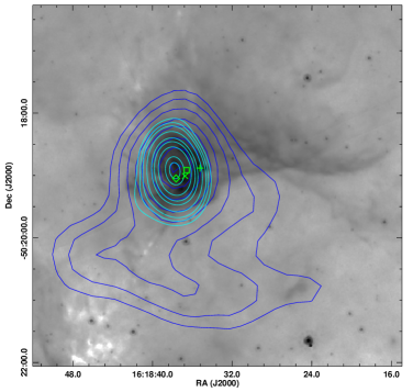
Figure 8: Spitzer 8.0 $\mu$m image of the region with overlaid 1280 MHz contours (at 3, 4, 5, 7, 10, 12, 15, 20, and 22 $\sigma$, where $\sigma\sim$ 8.85 mJy; resolution $\sim$ 56″$\times$35″ ) in cyan and 843 MHz contours (at 5, 7, 10, 15, 20, 30, 40, and 50 $\sigma$, where $\sigma\sim$ 5.57 mJy; resolution $\sim$ 56″$\times$43″ ) in blue. The symbols are same as for Fig. 7.

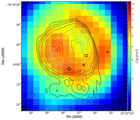
Figure 9: The colourmap Herschel 70 µm  image with overlaid 1280 MHz contours at 3, 4, 5, 7, 11, 13, 15, 17, 19, 20, and 21 $\sigma$ (where $\sigma\sim$ 0.4 mJy). The contours are from the maximum resolution (7″$\times$2″) radio continuum image that could be constructed at 1280 MHz. The symbols are same as Fig. 7.

Fig. 8 shows a $Spitzer$ 8.0 µm  image of the region with overlaid 843 MHz contours from MGPS and 1280 MHz contours from GMRT. Rest of the objects marked are same as in Fig. 7. The central core appears to be a compact H ii  region, near whose peak lie the mm peak and the high-mass source. The 843 MHz contours show extended emission in addition to the central compact region. The extended emission is only in the southern part and none in the northern part of the compact H ii  region, indicating the presence of dense molecular cloud in the northern part which is not ionized to the same extent as the southern region. The background 8.0 µm  image also shows the diffuse nebular emission in the north. Using the aips task jmfit, the compact cores at both the frequencies were fit with a Gaussian model to determine the source sizes and the fluxes. The obtained results are given in Table 3. The beam-deconvolved source size for MGPS 843 MHz is found to be much larger in area than that for 1280 MHz. The larger integrated flux density for 843 MHz could be because of this. Fig. 9 shows the maximum resolution image of the region which could be obtained at 1280 MHz ($\sim$7″$\times$2″), overlaid on the Herschel 70 µm  image. This contours show multiple peaks which is probably indicative of the clumpy nature of the ionized matter in the region. These peaks are mostly conincident with large 70 µm  emission, which is to be expected as 70 µm  also traces the thermal dust emission.

We tried to estimate the physical parameters of the region, using the lower resolution images, as follows. The Lyman continuum luminosity (in photons s^-1) required to generate the observed flux density was determined using the following formula (adapted from Kurtz, Churchwell, & Wood, 1994, see their Equations 1 and 3) :

$$S_{*}\geq\left(\frac{7.59\times 10^{48}}{a(\nu,T_{e})}\right)\left(\frac{S_{\nu}}{Jy}\right)\left(\frac{T_{e}}{K}\right)^{-0.5}\left(\frac{D}{kpc}\right)^{2}\left(\frac{\nu}{GHz}\right)^{0.1}$$ (3)

where $S_{\nu}$ is the integrated flux density in Jy, $D$ is the distance in kiloparsec, $T_{e}$ is the electron temperature, $a(\nu,T_{e})$ is the correction factor, and $\nu$ is the frequency in GHz at which the luminosity is to be calculated. The dynamical age of the H ii  region ($t$) can be solved for by using the following equation from Spitzer (1978) :

$$R(t)=R_{s}\left(1+\frac{7c_{II}t}{4R_{s}}\right)^{4/7}$$ (4)

where $R(t)$ is the radius of the H ii region at time $t$, $c_{II}$ is the speed of sound in H ii  region (11$\times$10⁵ cm s^-1; Stahler & Palla, 2005), and $R_{s}$ is the Strömgren radius. The Strömgren radius ($R_{s}$, in cm) is given by (Strömgren, 1939) :

$$R_{s}=\left(\frac{3S_{*}}{4\pi n_{o}^{2}\beta_{2}}\right)^{1/3}$$ (5)

where $n_{o}$ is the initial ambient density (in cm^-3), and $\beta_{2}$ is the total recombination coefficient to the first excited state of hydrogen. For our calculation, we assume a typical value of 10000 K for $T_{e}$ (which will imply a value of 0.99 for the correction factor ‘$a$’ ; see Table 6 of Mezger & Henderson, 1967), and the corresponding $\beta_{2}$ of 2.6$\times$10^-13 cm³ s^-1 (Stahler & Palla, 2005). For $n_{o}$, we use the value of 4.8$\times$10⁴ cm^-3 from Beltrán et al. (2006). $R(t)$ is taken as the geometric mean of fitted Gaussian source sizes from Table 3. Using these formulae and the 1280 MHz data, we calculated $S_{*}$ and $t$ as $\sim$ 10^47.41 photons s^-1 and $\sim$ 0.3 Myr, respectively. If we were to use the 843 MHz flux density data point, then $S_{*}$ and $t$ come out to be $\sim$ 10^47.73 photons s^-1 and $\sim$ 0.5 Myr, respectively. Assuming ZAMS, a comparison of $\log S_{*}$ with the tabulated values from Panagia (1973) shows that a spectral type of B0-O9.5 corresponds to this luminosity. Recent calibrations, like Martins, Schaerer, & Hillier (2005), also suggest a (luminosity class V) spectral type of $\sim$ O9.5. So, it seems that the spectral type of the source ionizing the region (assuming a single source) has to be earlier than B0-O9.5 for the ionization in the nebula to be sustained, since there can be absorption of ionizing photons by dust in the region which is often significant (Arthur et al., 2004). The dynamical age is approximately of the order of a few tenths of Myr.

We also try to fit to our data the free-free emission model of Mezger & Henderson (1967), according to which (adapted from Mezger, Schraml, & Terzian, 1967) :

$$S_{\nu}/\Omega=3.07\times 10^{-2}T_{e}\nu^{2}(1-e^{-\tau(\nu)})$$ (6)

$$\tau(\nu)=1.643\times 10^{5}a(\nu,T_{e})T_{e}^{-1.35}\nu^{-2.1}n_{e}^{2}l$$ (7)

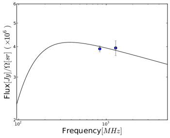
Figure 10: The fitted free-free emission model for the H ii  region. The data points at 843 MHz and 1280 MHz have been marked with solid circles.

where, $S_{\nu}$ is the integrated flux density (in Jy), $\nu$ is the frequency (in MHz), $n_{e}$ is the electron density in cm^-3, $l$ is the extent of the ionized region in pc, $\tau$ is the optical depth, and $\Omega$ is the solid angle subtended by the source (in steradians). $n_{e}^{2}l$ measures the optical depth in the medium (in cm^-6 pc), and is called the emission measure. Taking $\Omega$ as ($1.133\times\theta_{major}\times\theta_{minor}$), and the two data points, we fit the above equation using non-linear regression keeping $n_{e}^{2}l$ - the emission measure - as a free parameter. The fit is shown in Fig. 10. The emission measure is thus determined to be $\sim$ 4.00 $\pm$ 0.09 $\times$ 10⁴ cm^-6 pc. Since most of the central radio emission is confined within a circle of 120″  diameter, we can assume it to be the extent of the H ii  region ($\sim$ 2.1 pc), and thus the electron density ($n_{e}$) turns out to be $\sim$ 138 $cm^{-3}$. Further, using the formula from Mezger, Schraml, & Terzian (1967, Equation A.5), we calculate the total mass of ionized hydrogen (M${}_{\rm H\textsc{ii}}$) to be $\sim$ 16.4 $~{}M_{\odot}$ . These low values of $n_{e}$ and M${}_{\rm H\textsc{ii}}$, as well as the extent, would suggest that this region might be slightly more evolved than a compact H ii  region (Kurtz & Franco, 2002).

4.3 Central region

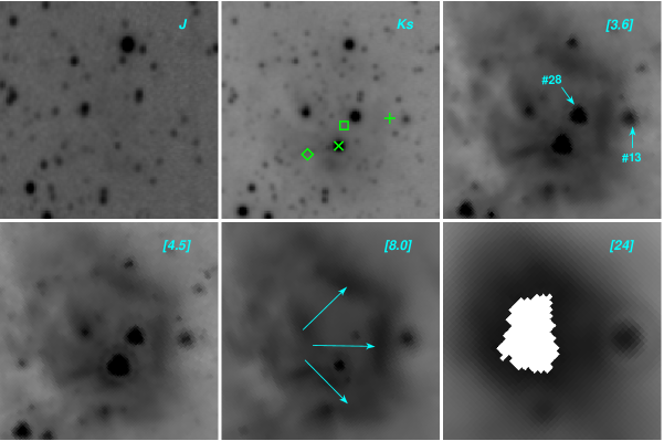
Figure 11: 1′ $\times$ 1′  central region of IRAS 16148-5011. The images (left-to-right, top-to-bottom) are $J$, $K_{s}$, 3.6 µm , 4.5 µm , 8.0 µm , and 24 µm . North is up and east is to the left. The symbols on the $K_{s}$ band image are same as Fig. 7 (green cross is #16 from Table 2). The numbered sources on the 3.6 µm  image are from Table 2. The cyan arrows on the 8.0 µm  image mark the ‘ring-like’  morphology. The white patch on the 24 µm  image is the saturated region.

Fig. 11 shows the central 1′ $\times$ 1′  region of IRAS 16148-5011 in the NIR $J$ and $K_{s}$ bands, IRAC 3.6 µm , 4.5 µm , and 8.0 µm  bands, and the MIPS 24 µm  band. The IRAC 3.6 µm  and 8.0 µm  bands, besides the continuum emission, also encompass the weak PAH emission feature at 3.3 µm , and strong PAH features at 7.7 µm  and 8.6 µm . The 4.5 µm  band does not contain any PAH features, but does contain shocked molecular gas emission from $H_{2}(v=0-0)~{}S(9,10,11)$ and $CO(v=1-0)$. 24 µm  emission is mainly the thermal continuum emission from the hot dust (Watson et al., 2008; Churchwell et al., 2009).

The $K_{S}$ band image has been marked with, among others, the high-mass source detected (green cross, #16 in Table 2) and the MSX peak from Molinari et al. (2008, ‘IRAS 16148-5011 A’) (green box). The marked high-mass source is of $\sim$ B2-B3 spectral type (as per tabulated values from Stahler & Palla, 2005, see their Table 1.1), while the radio flux suggests an ionizing star of type $\geq$ B0-O9.5. In addition, Molinari et al. (2008), using SED modelling (assuming an embedded ZAMS source) and the MSX flux values, have estimated the spectral type of ‘IRAS 16148-5011 A’  source as O8. Therefore, it appears that there could be further embedded high-mass source(s) in this region, in addition to those seen in NIR and MIR, for the values to be consistent. It is possible that the cores seen by radio contours in Fig. 9 could be hosting such high-mass source(s) and contributing to the radio luminosity.

The other sources associated with this central part of the nebula have been marked on the 3.6 µm  image (#13 and #28 from Table 2, Section 3.2). The source #13 appears to be a highly embedded intermediate-mass young source ($\sim$ 6.17 $~{}M_{\odot}$ , $\sim$ a few 10⁴ yr; see Section 3.2), even visible at 24 µm. Source #28 appears to be a much older and evolved source ($\sim$ 8.48 $~{}M_{\odot}$ , $\sim$ a few 10⁶ yr), possibly shrouded in the surrounding nebulosity (interstellar extinction of A${}_{V}\sim$ 18.38 mag), leading to a lack of detection in the $J$ band (though it is the second brightest source after the 9.6 $~{}M_{\odot}$  - #16 from Table 2 - source in the central region in $K_{s}$ band). The radio continuum emission contribution from this source will be much lower, hardly making a difference even when taken in combination with the emission from the high-mass source, and thus will not affect the inferences regarding radio emission above.

For H ii  regions, the PAH emissions serve as useful diagnostic tools as they are characteristic of photo-dissociation regions (PDRs). As a high-mass star ionizes its natal medium, the UV radiation destroys the PAH in its surroundings. However, at the boundary of the H ii  region produced, the UV intensity falls off, and a PDR is formed where the PAH’s are merely highly excited, leading to strong emission (Povich et al., 2007). The PDR is supposed to be the transition region between the ionized and neutral matter. This usually results in a ‘bubble’  morphology, where H ii  regions surrounded by ring-like PAH emission are seen (Churchwell et al., 2006). A similar morphology can be seen in the 3.6 µm  and the 8.0 µm  image in Fig. 11. A ‘semi-ring’  in the western half of the image is seen (marked by cyan arrows on the 8.0 µm  image). We note that this feature is also faintly seen in the 4.5 µm  image, though this could just be continuum emission. That this ring-like feature does not appear symmetric (i.e. there is no clear eastern ‘semi-ring’ , though faint indications are seen) could possibly be due to eastern denser and/or non-homogeneous molecular cloud, or projection effects. Volk et al. (1991), on the basis of low-resolution spectra, had classified IRAS 16148-5011 as a PAH source. Bulk of the radio emission (see Fig. 8), as well as the 24 µm  emission from hot dust, is confined within this ring-like feature as expected (Watson et al., 2008). Some of the emission from this ring-like structure could also be due to swept-up material by the expanding ionization front of the H ii  region.

4.4 Herschel Results

Thermal emission from cold dust lies in the FIR wavelength range, and thus its analysis can be used to obtain the physical parameters like dust temperature and column density of a region (Launhardt et al., 2013; Battersby et al., 2011). This was carried out by the SED modelling of the thermal dust emission, whose Rayleigh-Jeans regime is covered by the Herschel FIR bands (160–500 µm), using the following order of steps.

First of all, the surface brightness unit for all the images was converted to Jy pixel^-1. Since the PACS image is already in Jy pixel^-1, this step was only required for the SPIRE images (whose units are in MJy sr^-1), and was carried out using the pixel scales for the respective SPIRE bands. Next, the 160-350 µm  images were convolved to the resolution of the 500 µm  image ($\sim$ 36″ , lowest among all images) using the convolution kernels of Aniano et al. (2011), and regridded to a pixel scale of 14 ″  (same as 500 µm  image). Using these final reworked images with same resolution and pixel scale, a background flux level, $I_{bg}$, was determined from a “smooth”  (i.e. no abrupt clumpy regions) and relatively “dark”  patch of the sky. The distribution of individual pixel values in the dark patch of the sky, for each of the bands, was fitted with a Gaussian iteratively, rejecting the pixel values outside $\pm$ 2$\sigma$ in each iteration, till the fit converged. The same patch of the sky was used for each band. The background flux level, $I_{bg}$, was thus determined as 0.29, 2.67, 1.27, and 0.45 Jy pixel^-1 for the 160 µm, 250 µm, 350 µm, and 500 µm  images, respectively. We note that the 70 µm  image, though available, was not used here as the optically thin assumption might not hold true at this wavelength (Lombardi et al., 2014).

Modified blackbody fitting was subsequently carried out on a pixel-by-pixel basis using the following formulation (Battersby et al., 2011; Sadavoy et al., 2012; Nielbock et al., 2012; Launhardt et al., 2013) :

$$S_{\nu}(\nu)-I_{bg}(\nu)=B_{\nu}(\nu,T_{d})\Omega(1-e^{-\tau(\nu)}),$$ (8)

with

$$\tau(\nu)=\mu_{H_{2}}m_{H}\kappa_{\nu}N(H_{2}),$$ (9)

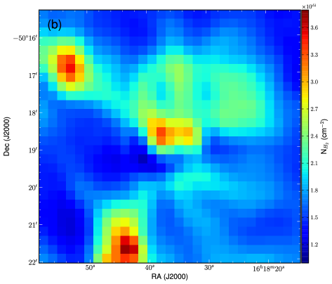
Figure 12: (a) Dust temperature map, and (b) column density map of the region around IRAS 16148-5011, derived using the SED fitting to the thermal dust emission.

where, $\nu$ is the frequency, $S_{\nu}(\nu)$ is the observed flux density, $I_{bg}(\nu)$ is the background flux in that particular band (estimated above), $B_{\nu}(\nu,T_{d})$ is the Planck’s function, $T_{d}$ is the dust temperature, $\Omega$ is the solid angle (in steradians) from where the flux is obtained (just the solid angle subtended by a 14″ $\times$14″  pixel here), $\tau(\nu)$ is the optical depth, $\mu_{H_{2}}$ is the mean molecular weight (adopted as 2.8 here), $m_{H}$ is the mass of hydrogen, $\kappa_{\nu}$ is the dust opacity, and $N(H_{2})$ is the column density. For opacity, we adopt a functional form of $\kappa_{\nu}=0.1$ $(\nu/1000$ GHz$)^{\beta}$ cm² g^-1, with $\beta=2$ (see André et al. 2010, Beckwith et al. 1990, Hildebrand 1983). For each pixel, Equation 8 was fit using the 4 data points, keeping $T_{d}$ and $N(H_{2})$ as free parameters. Pixels for which the fit did not converge, or the error was larger than 10%, had their values taken as the median of 8 immediate-neighbour pixels. The final obtained temperature and column density maps of the wider region (to clearly discern the morphological features) surrounding IRAS 16148-5011 are shown in Fig. 12.

From the temperature (Fig. 12) and column density (Fig. 12) maps, we obtain the peak values as $\sim$ 30 K and 3.3$\times$10²² cm^-2, respectively, for IRAS 16148-5011. Fontani et al. (2005) provide a temperature of 38 K (using greybody fit with 60 µm , 100 µm , and 1.2 mm data), and a (beam-averaged) column density of 3$\times$10²³ cm^-2 (using C¹⁷O molecular line observations) for IRAS 16148-5011. Here our peak temperature is about 20% lower, and the column density estimate an order of magnitude smaller. The difference in temperature seems to be due to their fitting limitations owing to sparse data points, as well as the fact that the 60 µm  emission might not be optically thin. It should be noted, however, that the dust temperature distribution from Fontani et al. (2005) (for their analysed catalogue of IRAS sources) peaks at $\sim$ 30 K. Column density disparity can probably be explained by the dependence of Fontani et al. (2005) on the molecular abundance of the rare C¹⁷O, whose value can have wide variations (Redman et al., 2002; Walsh et al., 2010).

The column density map (Fig. 12) displays three peaks - the central IRAS 16148-5011 object, a peak to its north-east, and a peak to its south. These north-east and south peaks appear to be associated with cold clumps, as is evident from the temperature map which shows T${}_{d}<20$ K at their positions. The column density map shows that all the peaks appear to be connected by weak filamententary features, similar to previous results for myriad regions (see André, 2013, and references therein). For the central IRAS 16148-5011 object, we estimated the associated clump dimensions, using the “clumpfind”  software (Williams, de Geus, & Blitz, 1994), to be $\sim$ 62″$\times$46″  (i.e. 1.1 pc$\times$0.8 pc at 3.6 kpc). Due to the low resolution of the column density image generated here, it does not appear possible to resolve further sub-clumps. The mass of the clump can be estimated by :

$$M_{clump} = \mu_{H_{2}}~{}m_{H}~{}\Sigma~{}N(H_{2})~{}Area_{pixel}$$ (10)

$$= \mu_{H_{2}}~{}m_{H}~{}Area_{pixel}~{}\Sigma~{}N(H_{2})$$ (11)

i.e. calculating the mass in each pixel and then summing over all the pixels which constitute the clump. Using the $\Sigma~{}N(H_{2})$ returned by the “clumpfind”  software, the total clump mass was calculated to be $\sim$ 1023 $~{}M_{\odot}$.

Another noticeable feature in this map is that the immediate northern vicinity of the central region exhibits higher column density than the immediate southern portion. This suggests dense nebula in the northern part, affirming the inference also drawn from extinction and cluster analysis in Section 4.1 (also see Fig. 7). This is also consonant with the fact that the dense nebular emission is in the northern part, with no extended radio emission seen there (unlike in the southern part). To get an estimate of the visual extinction in this northern part, we use the relation $\langle N(H_{2})/A_{V}\rangle$=0.94$\times$10²¹ molecules cm^-1 mag^-1 (adapted from Bohlin, Savage, & Drake, 1978, assuming a total-to-selective extinction ratio $R_{V}$=3.1, and that the gas is in molecular form). Now, typical N(H₂) seen here is $\gtrsim$ 2$\times$10²² cm^-3, which implies an A${}_{V}>20$ mag. This high value of A_V is probably the reason why very few YSOs are associated with this northern nebular emission (see Fig. 7). If the value of R_V were to be larger, as has been conjectured for dense environments, then it will lead to an increase in A_V.

5 Discussion

The IRAS 16148-5011 region appears to be hosting an infrared cluster containing high-mass star(s) embedded in the nebula, and could serve as a future template to study the high-mass star formation process. Age estimates for any cluster are usually plagued with uncertainties (see Lada & Lada, 2003, for a discussion), and various proxies are often used to ascertain the evolutionary stage of a cluster. One such is the ratio of Class II to Class I sources (as Class II sources are older) (Schmeja, Klessen, & Froebrich, 2005; Beerer et al., 2010; Gutermuth et al., 2009). We have detected 133 Class II and 7 Class I sources in this region. However, here it seems that the large ratio (19) could be because Class I sources are deeply embedded and their detection is affected by large nebular extinction, though varying ratio values have been estimated for other clusters (Gutermuth et al., 2009).

The two brightest (NIR) sources in the central region appear to be high-mass (see Section 4.3) with indications of futher embedded high-mass sources. Also in literature, Beltrán et al. (2006) report two clumps within 90″  of the IRAS 16148-5011 IRAS catalogue position - ‘16148-5011 Clump 2’  (206 $~{}M_{\odot}$) and ‘16148-5011 Clump 3’  (42 $~{}M_{\odot}$) - detected using 1.2 mm emission and a dust temperature of 30 K. While ‘Clump 2’ , is almost coincident with the ‘16148-5011 MM 1’  peak from Molinari et al. (2008) (marked with a diamond symbol on Fig. 11), ‘Clump 3’  coordinates are same as the IRAS 16148-5011’s IRAS catalogue coordinates (green plus in Fig. 11). The presence of these massive clumps could also point towards ongoing high-mass star formation in the region.

Though this part of the sky also harbours other IRAS sources (Karnik et al., 2001), IRAS 16148-5011 does not appear to be a part of any larger star-forming complex as such, but it seems to be connected to other clumps via filaments (similar to the hub-filament morphology of Myers, 2009). The high-mass stellar cluster formation in the associated molecular cloud appears to be spontaneous. However, along the rather sharp southern boundary of the molecular cloud, the results from cluster analysis show a stellar sub-cluster forming (Fig. 7), which could partly be due to the triggering by the expanding ionization front of the H ii  region.

6 Conclusions

The main conclusions of this paper, resulting from a multiwavelength study involving NIR, MIR, FIR, and radio continuum data, are as follows :

1. 7 Class I and 133 Class II YSOs are identified using a combination of NIR and MIR data. A 9.6 $~{}M_{\odot}$  high-mass source is found to be associated with the central nebula.

2. Low-frequency radio emission reveals a compact H ii  region, with extended emission in the southern part. Lyman continuum photon luminosity calculation gives B0-O9.5 as the lower limit for the spectral type of the ionizing source (assuming single source). The dynamical age of the H ii  region is in 0.3-0.5 Myr range. SED modelling of the free-free emission yields an electron density of 138 cm^-3. The mass of the ionized hydrogen is calculated to be $\sim$ 16.4 $~{}M_{\odot}$. The high-resolution 7″$\times$2″  contour map shows clumpy ionized gas in the region.

3. The central nebular region shows a ring-like PAH emission feature near the borders of the compact H ii  region, tracing the PDR. There appear to be three NIR- and MIR-visible central sources, of masses $\sim$ 6.2 $~{}M_{\odot}$, 9.60 $~{}M_{\odot}$, and 8.5 $~{}M_{\odot}$. Based on the incongruency between the total radio flux from these sources and the flux obtained from radio observations, and literature estimates of an early type star using MIR SED fitting, it is possible that there could be high-mass embedded source(s) present in this region.

4. Dust temperature and column density maps are obtained using SED modelling of the thermal dust emission. The peak temperature and column density values are 30 K and 3.3$\times$10²² cm^-2, respectively, for IRAS 16148-5011. The column density map reveals that the immediate northern vicinity of IRAS 16148-5011, which contains the nebular emission seen prominently at MIR wavelengths, has a large extinction of A${}_{V}>$ 20 mag. This map also shows that weak filamententary structures join IRAS 16148-5011 to nearby cold clumps. The size and mass of the clump associated with IRAS 16148-5011 is estimated to be $\sim$ 1.1 pc$\times$0.8 pc (at 3.6 kpc) and $\sim$ 1023 $~{}M_{\odot}$, respectively.

Future observations of individual objects in spectral lines, deeper IR data to get a full stellar census upto below brown-dwarf limit, further molecular line observations which probe high column densities will help put the star formation scenario on a firm footing and help study high-mass star formation.

Table 1: YSOs identified using NIR and MIR data

RA	Dec.	$J$	$H$	$K_{s}$	$[3.6]$	$[4.5]$	$[5.8]$	$[8.0]$	YSO
(J2000)	(J2000)	(mag)	(mag)	(mag)	(mag)	(mag)	(mag)	(mag)	Classification
244.575165	-50.365025	17.861 $\pm$ 0.130	16.631 $\pm$ 0.001	15.509 $\pm$ 0.047	14.311 $\pm$ 0.145	14.132 $\pm$ 0.203	—	—	Class2
244.575241	-50.367393	14.580 $\pm$ 0.021	13.876 $\pm$ 0.010	13.643 $\pm$ 0.032	12.983 $\pm$ 0.099	12.872 $\pm$ 0.122	—	—	Class2
244.576645	-50.293938	16.137 $\pm$ 0.016	14.443 $\pm$ 0.010	13.570 $\pm$ 0.020	12.780 $\pm$ 0.102	12.372 $\pm$ 0.132	—	—	Class2
244.577545	-50.314171	15.557 $\pm$ 0.010	14.358 $\pm$ 0.010	13.818 $\pm$ 0.028	13.001 $\pm$ 0.108	12.820 $\pm$ 0.143	—	—	Class2
244.579193	-50.321396	17.491 $\pm$ 0.045	15.921 $\pm$ 0.020	14.881 $\pm$ 0.038	13.412 $\pm$ 0.161	13.265 $\pm$ 0.132	—	—	Class2

Table 1 is available in its entirety in a machine-readable form in the online journal. A portion is shown here for guidance regarding its form and content.

Table 2: Main parameters from SED analysis

S.No.	RA	Dec.	$\log\,t_{*}$	Mass	$\log\,M_{disk}$	$\log\,\dot{M}_{disk}$	$\log\,M_{env}$	$\log\,T_{*}$	$\log\,L_{total}$	$A_{V}$	$\chi_{min}^{2}$
	(J2000)	(J2000)	($yr$)	($M_{\odot}$)	($M_{\odot}$)	($M_{\odot}~{}yr^{-1}$)	($M_{\odot}$)	(K)	($L_{\odot}$)	(mag)	(per data point)
Class I sources
1	244.591080	-50.285355	6.33 $\pm$ 0.74	2.42 $\pm$ 0.79	-3.38 $\pm$ 1.64	-9.29 $\pm$ 1.73	-4.43 $\pm$ 2.73	3.85 $\pm$ 0.15	1.41 $\pm$ 0.30	4.81 $\pm$ 2.35	0.29
2	244.603455	-50.292828	4.71 $\pm$ 0.40	4.20 $\pm$ 1.42	-1.39 $\pm$ 0.70	-6.70 $\pm$ 0.99	0.68 $\pm$ 1.06	3.66 $\pm$ 0.07	2.11 $\pm$ 0.28	15.95 $\pm$ 4.98	0.01
3	244.671539	-50.338348	5.30 $\pm$ 1.02	2.58 $\pm$ 1.61	-2.90 $\pm$ 1.82	-8.08 $\pm$ 2.02	-2.70 $\pm$ 2.90	3.73 $\pm$ 0.20	1.56 $\pm$ 0.56	7.45 $\pm$ 4.16	0.10
Class II sources
4	244.584152	-50.353664	4.65 $\pm$ 0.37	6.41 $\pm$ 0.54	-2.12 $\pm$ 0.75	-6.94 $\pm$ 0.80	1.65 $\pm$ 0.40	3.66 $\pm$ 0.01	2.49 $\pm$ 0.06	12.17 $\pm$ 5.81	9.90
5	244.599808	-50.286560	4.94 $\pm$ 0.37	3.80 $\pm$ 1.81	-1.99 $\pm$ 0.84	-7.55 $\pm$ 1.30	0.54 $\pm$ 0.66	3.66 $\pm$ 0.05	1.93 $\pm$ 0.41	11.51 $\pm$ 5.27	1.93
6	244.606796	-50.307327	5.57 $\pm$ 0.87	7.50 $\pm$ 3.12	-4.67 $\pm$ 2.72	-9.18 $\pm$ 2.08	-3.10 $\pm$ 4.21	4.02 $\pm$ 0.35	2.95 $\pm$ 0.68	13.72 $\pm$ 5.07	5.34
7	244.609207	-50.351631	4.97 $\pm$ 0.27	4.68 $\pm$ 1.40	-2.11 $\pm$ 0.93	-7.66 $\pm$ 1.31	1.24 $\pm$ 0.53	3.67 $\pm$ 0.05	2.12 $\pm$ 0.32	17.37 $\pm$ 3.72	10.85
8	244.610397	-50.279411	5.14 $\pm$ 0.76	2.99 $\pm$ 1.59	-2.25 $\pm$ 0.95	-7.76 $\pm$ 1.28	-0.70 $\pm$ 2.22	3.70 $\pm$ 0.15	1.73 $\pm$ 0.36	13.43 $\pm$ 5.74	0.29
9	244.612305	-50.365067	4.84 $\pm$ 0.45	5.60 $\pm$ 2.59	-2.04 $\pm$ 1.05	-7.61 $\pm$ 1.55	1.09 $\pm$ 0.87	3.70 $\pm$ 0.07	2.31 $\pm$ 0.66	4.51 $\pm$ 2.81	0.34
10	244.614349	-50.327496	6.28 $\pm$ 0.66	2.50 $\pm$ 0.83	-3.40 $\pm$ 1.71	-9.21 $\pm$ 1.89	-4.37 $\pm$ 2.56	3.85 $\pm$ 0.17	1.44 $\pm$ 0.35	6.20 $\pm$ 2.30	0.13
11	244.633514	-50.326122	5.73 $\pm$ 0.70	2.58 $\pm$ 0.99	-3.20 $\pm$ 1.77	-8.84 $\pm$ 1.80	-2.83 $\pm$ 2.80	3.77 $\pm$ 0.19	1.54 $\pm$ 0.35	8.83 $\pm$ 4.50	0.28
12	244.639954	-50.283981	5.10 $\pm$ 0.07	4.80 $\pm$ 0.22	-2.36 $\pm$ 0.66	-7.50 $\pm$ 0.20	1.14 $\pm$ 0.56	3.66 $\pm$ 0.01	2.02 $\pm$ 0.07	9.75 $\pm$ 5.38	2.16
13a,b	244.644714	-50.314804	4.18 $\pm$ 1.01	6.17 $\pm$ 1.74	-	-	-0.18 $\pm$ 1.92	3.76 $\pm$ 0.26	2.82 $\pm$ 0.31	6.18 $\pm$ 3.86	0.03
14	244.649155	-50.346909	5.65 $\pm$ 0.90	2.44 $\pm$ 1.12	-2.92 $\pm$ 1.44	-8.40 $\pm$ 1.68	-2.87 $\pm$ 3.05	3.79 $\pm$ 0.20	1.58 $\pm$ 0.35	7.63 $\pm$ 4.29	0.03
15	244.651047	-50.328751	6.29 $\pm$ 0.68	3.46 $\pm$ 0.86	-3.43 $\pm$ 1.48	-8.96 $\pm$ 1.60	-4.83 $\pm$ 2.75	3.99 $\pm$ 0.18	2.01 $\pm$ 0.27	6.70 $\pm$ 2.41	0.13
16a,c	244.652878	-50.316849	5.44 $\pm$ 0.61	9.60 $\pm$ 1.44	-2.15 $\pm$ 1.24	-7.00 $\pm$ 1.35	0.00 $\pm$ 3.42	4.29 $\pm$ 0.20	3.69 $\pm$ 0.16	15.97 $\pm$ 4.36	0.89
17	244.663803	-50.352959	6.02 $\pm$ 0.78	2.93 $\pm$ 0.82	-3.23 $\pm$ 1.35	-8.92 $\pm$ 1.53	-3.75 $\pm$ 3.08	3.86 $\pm$ 0.19	1.74 $\pm$ 0.24	4.75 $\pm$ 2.79	0.07
18	244.671738	-50.278400	5.30 $\pm$ 0.28	3.02 $\pm$ 1.19	-2.97 $\pm$ 1.18	-8.96 $\pm$ 1.72	-0.74 $\pm$ 0.91	3.67 $\pm$ 0.05	1.62 $\pm$ 0.27	10.13 $\pm$ 3.37	3.23
19	244.679535	-50.293499	4.97 $\pm$ 0.36	4.10 $\pm$ 1.47	-2.07 $\pm$ 0.86	-7.70 $\pm$ 1.19	0.45 $\pm$ 0.86	3.67 $\pm$ 0.06	2.01 $\pm$ 0.30	9.06 $\pm$ 5.71	2.25
20	244.685440	-50.357010	6.29 $\pm$ 0.72	3.69 $\pm$ 0.99	-3.83 $\pm$ 1.67	-9.31 $\pm$ 1.77	-5.06 $\pm$ 2.77	4.03 $\pm$ 0.19	2.14 $\pm$ 0.32	9.15 $\pm$ 3.12	0.17
21	244.689316	-50.343143	4.99 $\pm$ 0.39	3.85 $\pm$ 1.38	-2.13 $\pm$ 0.83	-7.74 $\pm$ 1.20	0.28 $\pm$ 1.05	3.67 $\pm$ 0.06	1.94 $\pm$ 0.26	7.45 $\pm$ 5.58	2.23
22	244.689453	-50.366440	4.90 $\pm$ 0.48	4.06 $\pm$ 1.33	-1.97 $\pm$ 0.87	-7.40 $\pm$ 1.17	0.37 $\pm$ 1.39	3.67 $\pm$ 0.09	2.04 $\pm$ 0.26	13.02 $\pm$ 5.40	0.17
23	244.693146	-50.279778	5.50 $\pm$ 0.67	2.95 $\pm$ 0.96	-2.39 $\pm$ 0.94	-8.01 $\pm$ 1.08	-1.47 $\pm$ 2.53	3.73 $\pm$ 0.16	1.68 $\pm$ 0.19	7.19 $\pm$ 3.64	4.84
24	244.704742	-50.351349	4.78 $\pm$ 0.39	5.70 $\pm$ 0.86	-2.26 $\pm$ 0.30	-7.61 $\pm$ 0.94	1.65 $\pm$ 0.30	3.66 $\pm$ 0.02	2.37 $\pm$ 0.09	17.61 $\pm$ 2.63	14.26
25	244.708603	-50.286385	4.89 $\pm$ 0.35	4.59 $\pm$ 1.48	-1.92 $\pm$ 0.84	-7.52 $\pm$ 1.14	0.89 $\pm$ 0.71	3.67 $\pm$ 0.06	2.14 $\pm$ 0.34	12.96 $\pm$ 5.63	3.55
26	244.683786	-50.363702	4.75 $\pm$ 0.39	6.24 $\pm$ 2.25	-1.56 $\pm$ 0.82	-6.91 $\pm$ 1.09	1.25 $\pm$ 0.72	3.71 $\pm$ 0.11	2.52 $\pm$ 0.51	6.59 $\pm$ 5.53	1.57
27	244.687016	-50.353573	5.46 $\pm$ 0.73	2.87 $\pm$ 1.67	-2.60 $\pm$ 1.34	-8.20 $\pm$ 1.54	-1.73 $\pm$ 2.66	3.74 $\pm$ 0.16	1.62 $\pm$ 0.50	12.36 $\pm$ 6.40	0.01
Extra central source
28a,b	244.650894	-50.314579	6.17 $\pm$ 0.35	8.48 $\pm$ 1.17	-4.25 $\pm$ 1.30	-9.31 $\pm$ 1.32	-4.20 $\pm$ 3.65	4.36 $\pm$ 0.06	3.52 $\pm$ 0.21	18.38 $\pm$ 2.26	3.09

$a$ : Prominent sources associated with the central nebula; $b$ : Did not have 8.0 µm  photometry; $c$ : Identified as “G333.0494+00.0324B”  (and also classified as a YSO) in Lumsden et al. (2013).

Table 3: Fitting results for compact H ii  region

	1280 MHz	843 MHz
2-D Gaussian fit
size	60.30″$\times$39.71″	69.41″$\times$76.17″
Beam-deconvolved
source size	23.35″$\times$18.31″	51.25″$\times$54.97″
Position Angle (deg)	160.1	128.2
Peak flux
density (mJy beam-1)	204$\pm$9	258$\pm$5
Integrated flux
density (mJy)	252$\pm$18	552$\pm$16

References

- Anderson et al. (2012) Anderson L. D., et al., 2012, A&A, 542, A10
- André et al. (2010) André P., et al., 2010, A&A, 518, L102
- André (2013) André P., 2013, arXiv, arXiv:1309.7762
- Aniano et al. (2011) Aniano G., Draine B. T., Gordon K. D., Sandstrom K., 2011, PASP, 123, 1218
- Arthur et al. (2004) Arthur S. J., Kurtz S. E., Franco J., Albarrán M. Y., 2004, ApJ, 608, 282
- Balog et al. (2004) Balog Z., Kenyon S. J., Lada E. A., Barsony M., Vinkó J., Gáspaŕ A., 2004, AJ, 128, 2942
- Battersby et al. (2011) Battersby C., et al., 2011, A&A, 535, A128
- Beckwith et al. (1990) Beckwith S. V. W., Sargent A. I., Chini R. S., Guesten R., 1990, AJ, 99, 924
- Beerer et al. (2010) Beerer I. M., et al., 2010, ApJ, 720, 679
- Beltrán et al. (2006) Beltrán M. T., Brand J., Cesaroni R., Fontani F., Pezzuto S., Testi L., Molinari S., 2006, A&A, 447, 221
- Benjamin et al. (2003) Benjamin R. A., et al., 2003, PASP, 115, 953
- Bessell & Brett (1988) Bessell M. S., Brett J. M., 1988, PASP, 100, 1134
- Bohlin, Savage, & Drake (1978) Bohlin R. C., Savage B. D., Drake J. F., 1978, ApJ, 224, 132
- Cantalupo et al. (2010) Cantalupo C. M., Borrill J. D., Jaffe A. H., Kisner T. S., Stompor R., 2010, ApJS, 187, 212
- Carpenter (2001) Carpenter J. M., 2001, AJ, 121, 2851
- Casertano & Hut (1985) Casertano S., Hut P., 1985, ApJ, 298, 80
- Chan, Henning, & Schreyer (1996) Chan S. J., Henning T., Schreyer K., 1996, A&AS, 115, 285
- Chavarría et al. (2008) Chavarría L. A., Allen L. E., Hora J. L., Brunt C. M., Fazio G. G., 2008, ApJ, 682, 445
- Churchwell et al. (2006) Churchwell E., et al., 2006, ApJ, 649, 759
- Churchwell et al. (2009) Churchwell E., et al., 2009, PASP, 121, 213
- Cohen et al. (1981) Cohen J. G., Persson S. E., Elias J. H., Frogel J. A., 1981, ApJ, 249, 481
- Dutra et al. (2003) Dutra C. M., Bica E., Soares J., Barbuy B., 2003, A&A, 400, 533
- Flaherty et al. (2007) Flaherty K. M., Pipher J. L., Megeath S. T., Winston E. M., Gutermuth R. A., Muzerolle J., Allen L. E., Fazio G. G., 2007, ApJ, 663, 1069
- Fontani et al. (2005) Fontani F., Beltrán M. T., Brand J., Cesaroni R., Testi L., Molinari S., Walmsley C. M., 2005, A&A, 432, 921
- Grave & Kumar (2009) Grave J. M. C., Kumar M. S. N., 2009, A&A, 498, 147
- Green et al. (1999) Green A. J., Cram L. E., Large M. I., Ye T., 1999, ApJS, 122, 207
- Griffin et al. (2010) Griffin M. J., et al., 2010, A&A, 518, L3
- Gutermuth et al. (2009) Gutermuth R. A., Megeath S. T., Myers P. C., Allen L. E., Pipher J. L., Fazio G. G., 2009, ApJS, 184, 18, Erratum : 2010, ApJS, 189, 352
- Haslam et al. (1982) Haslam C. G. T., Salter C. J., Stoffel H., Wilson W. E., 1982, A&AS, 47, 1
- Haynes, Caswell, & Simons (1979) Haynes R. F., Caswell J. L., Simons L. W. J., 1979, AuJPA, 48, 1
- Hildebrand (1983) Hildebrand R. H., 1983, QJRAS, 24, 267
- Hillenbrand et al. (1992) Hillenbrand L. A., Strom S. E., Vrba F. J., Keene J., 1992, ApJ, 397, 613
- Karnik et al. (2001) Karnik A. D., Ghosh S. K., Rengarajan T. N., Verma R. P., 2001, MNRAS, 326, 293
- Kurtz, Churchwell, & Wood (1994) Kurtz S., Churchwell E., Wood D. O. S., 1994, ApJS, 91, 659
- Kurtz & Franco (2002) Kurtz S., Franco J., 2002, RMxAC, 12, 16
- Lada (1987) Lada C. J., 1987, IAUS, 115, 1
- Lada et al. (1991) Lada E. A., Depoy D. L., Evans N. J., II, Gatley I., 1991, ApJ, 371, 171
- Lada & Adams (1992) Lada C. J., Adams F. C., 1992, ApJ, 393, 278
- Lada, Young, & Greene (1993) Lada C. J., Young E. T., Greene T. P., 1993, ApJ, 408, 471
- Lada et al. (1994) Lada C. J., Lada E. A., Clemens D. P., Bally J., 1994, ApJ, 429, 694
- Lada & Lada (1995) Lada E. A., Lada C. J., 1995, AJ, 109, 1682
- Lada & Lada (2003) Lada C. J., Lada E. A., 2003, ARA&A, 41, 57
- Launhardt et al. (2013) Launhardt R., et al., 2013, A&A, 551, A98
- Lombardi et al. (2014) Lombardi M., Bouy H., Alves J., Lada C. J., 2014, A&A, 566, A45, Erratum : 2014, A&A, 568, 1
- Lumsden et al. (2013) Lumsden S. L., Hoare M. G., Urquhart J. S., Oudmaijer R. D., Davies B., Mottram J. C., Cooper H. D. B., Moore T. J. T., 2013, ApJS, 208, 11
- MacLeod et al. (1998) MacLeod G. C., van der Walt D. J., North A., Gaylard M. J., Galt J. A., Moriarty-Schieven G. H., 1998, AJ, 116, 2936
- Mallick et al. (2013) Mallick K. K., Kumar M. S. N., Ojha D. K., Bachiller R., Samal M. R., Pirogov L., 2013, ApJ, 779, 113
- Mallick et al. (2014) Mallick K. K., et al., 2014, MNRAS, 443, 3218
- Martins, Schaerer, & Hillier (2005) Martins F., Schaerer D., Hillier D. J., 2005, A&A, 436, 1049
- Massey (1998) Massey P., 1998, ASPC, 142, 17
- Megeath (1996) Megeath S. T., 1996, A&A, 311, 135
- Meyer, Calvet, & Hillenbrand (1997) Meyer M. R., Calvet N., Hillenbrand L. A., 1997, AJ, 114, 288
- Mezger, Schraml, & Terzian (1967) Mezger P. G., Schraml J., Terzian Y., 1967, ApJ, 150, 807
- Mezger & Henderson (1967) Mezger P. G., Henderson A. P., 1967, ApJ, 147, 471
- Molinari et al. (2008) Molinari S., Pezzuto S., Cesaroni R., Brand J., Faustini F., Testi L., 2008, A&A, 481, 345
- Molinari et al. (2010) Molinari S., et al., 2010, PASP, 122, 314
- Mookerjea et al. (2004) Mookerjea B., Kramer C., Nielbock M., Nyman L.-Å., 2004, A&A, 426, 119
- Moran (1983) Moran J. M., 1983, RMxAA, 7, 95
- Myers (2009) Myers P. C., 2009, ApJ, 700, 1609
- Nagashima et al. (1999) Nagashima C., et al., 1999, sf99.proc, 397
- Nagayama et al. (2003) Nagayama T., et al., 2003, SPIE, 4841, 459
- Nielbock et al. (2012) Nielbock M., et al., 2012, A&A, 547, A11
- Ojha et al. (2004a) Ojha D. K., et al., 2004a, ApJ, 608, 797
- Ojha et al. (2004b) Ojha D. K., et al., 2004b, ApJ, 616, 1042
- Panagia (1973) Panagia N., 1973, AJ, 78, 929
- Persson et al. (1998) Persson S. E., Murphy D. C., Krzeminski W., Roth M., Rieke M. J., 1998, AJ, 116, 2475
- Pilbratt et al. (2010) Pilbratt G. L., et al., 2010, A&A, 518, L1
- Poglitsch et al. (2010) Poglitsch A., et al., 2010, A&A, 518, L2
- Povich et al. (2007) Povich M. S., et al., 2007, ApJ, 660, 346
- Redman et al. (2002) Redman M. P., Rawlings J. M. C., Nutter D. J., Ward-Thompson D., Williams D. A., 2002, MNRAS, 337, L17
- Robitaille et al. (2006) Robitaille T. P., Whitney B. A., Indebetouw R., Wood K., Denzmore P., 2006, ApJS, 167, 256
- Robitaille et al. (2007) Robitaille T. P., Whitney B. A., Indebetouw R., Wood K., 2007, ApJS, 169, 328
- Robitaille (2008) Robitaille T. P., 2008, ASPC, 387, 290
- Sadavoy et al. (2012) Sadavoy S. I., et al., 2012, A&A, 540, A10
- Samal et al. (2014) Samal M. R., et al., 2014, A&A, 566, A122
- Sanchawala et al. (2007) Sanchawala K., et al., 2007, ApJ, 667, 963
- Schmeja (2011) Schmeja S., 2011, AN, 332, 172
- Schmeja, Klessen, & Froebrich (2005) Schmeja S., Klessen R. S., Froebrich D., 2005, A&A, 437, 911
- Schmeja, Kumar, & Ferreira (2008) Schmeja S., Kumar M. S. N., Ferreira B., 2008, MNRAS, 389, 1209
- Sharma et al. (2007) Sharma S., Pandey A. K., Ojha D. K., Chen W. P., Ghosh S. K., Bhatt B. C., Maheswar G., Sagar R., 2007, MNRAS, 380, 1141
- Siess, Dufour, & Forestini (2000) Siess L., Dufour E., Forestini M., 2000, A&A, 358, 593
- Spitzer (1978) Spitzer L., 1978, ppim.book,
- Stahler & Palla (2005) Stahler S. W., Palla F., 2005, fost.book
- Strömgren (1939) Strömgren B., 1939, ApJ, 89, 526
- Swarup et al. (1991) Swarup G., Ananthakrishnan S., Kapahi V. K., Rao A. P., Subrahmanya C. R., Kulkarni V. K., 1991, CuSc, 60, 95
- Tej et al. (2006) Tej A., Ojha D. K., Ghosh S. K., Kulkarni V. K., Verma R. P., Vig S., Prabhu T. P., 2006, A&A, 452, 203
- Vig et al. (2014) Vig S., Ghosh S. K., Ojha D. K., Verma R. P., Tamura M., 2014, MNRAS, 440, 3078
- Volk et al. (1991) Volk K., Kwok S., Stencel R. E., Brugel E., 1991, ApJS, 77, 607
- Walsh et al. (2010) Walsh A. J., Thorwirth S., Beuther H., Burton M. G., 2010, MNRAS, 404, 1396
- Watson et al. (2008) Watson C., et al., 2008, ApJ, 681, 1341
- Williams, de Geus, & Blitz (1994) Williams J. P., de Geus E. J., Blitz L., 1994, ApJ, 428, 693
- Whitney et al. (2003a) Whitney B. A., Wood K., Bjorkman J. E., Cohen M., 2003, ApJ, 598, 1079
- Whitney et al. (2003b) Whitney B. A., Wood K., Bjorkman J. E., Wolff M. J., 2003, ApJ, 591, 1049
- Zinnecker & Yorke (2007) Zinnecker H., Yorke H. W., 2007, ARA&A, 45, 481
- Zinnecker, McCaughrean, & Wilking (1993) Zinnecker H., McCaughrean M. J., Wilking B. A., 1993, prpl.conf, 429