Higher derivative Chern-Simons extension in the noncommutative QED3

M. Ghasemkhani111e-mail: $m_{{}_{-}}$ghasemkhani@sbu.ac.ir${}^{;\ a}$ and R. Bufalo222e-mail: rodrigo.bufalo@helsinki.fi${}^{;\ b,c}$

a
Department of Physics, Shahid Beheshti University,
G.C., Evin, Tehran 19839, Iran
b
Department of Physics, University of Helsinki, P.O. Box 64
FI-00014 Helsinki, Finland
c
Instituto de FΓ­sica TeΓ³rica (IFT), Universidade Estadual Paulista
Rua Dr. Bento Teobaldo Ferraz 271, Bloco II, 01140-070 SΓ£o Paulo, SP, Brazil

The noncommutative (NC) massive quantum electrodynamics in $2+1$ dimensions is considered. We show explicitly that the one-loop effective action arising from the integrating out the fermionic fields leads to the ordinary NC Chern-Simons and NC Maxwell action at the long wavelength limit (large fermion mass). In the next to leading order, the higher-derivative contributions to NC Chern-Simons are obtained. Moreover, the gauge invariance of the outcome action is carefully discussed. We then consider the higher-derivative modification into the pure NC Chern-Simons Lagrangian density and evaluate the one-loop correction to the pole of the photon propagator.

1 Introduction

Low-dimensional field theories were recognized, a long time ago, as serving as laboratories where important theoretical ideas are suitably tested in a simple setting, specially on condensed matter systems. Besides, these studies were also driven with the wishful thought that in such simpler setting we can learn useful things about the well-recognized four-dimensional problems. Furthermore, including to that, the fact that a field theory defined in a three-dimensional space-time contains a highly interesting inner structure, due to the odd space-time dimensionality, it is rather natural to investigate them as theoretical options [2, 3, 4, 5].

Due to the recent improvement concerning the precision of the measurements of experiments (LHC, ILC, etc) investigating particles properties, the possibility of observing direct evidence of new physics has captured and led to a major interest in the development and understanding of the physics in higher scales, for instance at Planck scale. A conscientious point in the majority of the analyses is that the nature of the space-time may change at Planck scale. This fact had strong influence in thinking that the physics at Planck scale may suitably be described by a noncommutativity between the coordinates of the space-time. Direct motivations supporting considering models constructed on noncommutative space-time are many, and come from several theoretical areas such as string theory, quantum gravity, and Lorentz breaking [6, 7, 8].

In recent years, we have witnessed an enormous activity involving the development of noncommutative (NC) gauge theories in high-energy physics [6, 9]. The noncommutativity of space-time, whose structure is determined by $[x^{\mu},x^{\nu}]=i\theta^{\mu\nu}$, has provided a better understanding about the quantum nature of space-time. On the other hand, it has been also studied how noncommutativity affects established properties of conventional theories, i.e., studying NC extensions of well studied quantum field theories and to look then for NC effects on its deviations, since it is generally found that such extensions behave in a very interesting and nontrivial ways. Despite its close relation with the space-time structure, no consistent gravitational theory defined on noncommutative space-time has been established yet [10].

In fact, various studies in analyzing three-dimensional gauge theories defined in a noncommutative space-time have uncovered deviations of known phenomena and interesting new properties of these theories [11, 12, 13, 14, 15, 16, 17]. One of the most exploited features of a three-dimensional gauge theory is that, in one side, if you started with a theory with massless fermionic fields interacting with Chern-Simons gauge fields, a mass for the fermionic fields is generated dynamically by radiative corrections; on the other side, if you started with a theory with massive fermionic fields interacting with an external gauge field, the Chern-Simons action is also induced by radiative corrections. These properties are usually related to nonperturbative phenomena due to the space-time dimensionality.

The generation of the Chern-Simons action in a noncommutative gauge theory was the subject of several analyses, with the most different purposes [15, 17, 18, 19, 20, 21, 22]. However, no higher-derivative (HD) extensions of the Chern-Simons action have been considered. This subject was first discussed in great detail by considering the full Abelian action, consisting in the Chern-Simons added by the Maxwell theory, 111This theory is the so-called topologically massive electrodynamics [2], and describes a helicity $\pm 1$ mode., adjoined by higher-derivative contributions appearing from a $(\partial/m)$ perturbative expansion of the effective action of QED3 [23, 24]. Our main aim in the present paper is to treat the latter phenomenon in full detail when formulated within the framework of noncommutative gauge theory.

In this paper, we discuss, within the effective action approach, the one-loop properties of the three-dimensional noncommutative QED. For this purpose, we follow the idea outlined in Ref.[25] in which noncommutative fermionic effective actions were considered. Although the Seiberg-Witten map is perturbative by nature [6], remarkably, it suffices to consider the existence of an exact Seiberg-Witten map, valid to all orders in $\theta$, in a formal way that the noncommutative effects into the resulting outcome are in fact nonperturbative. For this purpose, in Sec.Β 2, we review the basic ideas consisting in this nonperturbative approach (in $\theta$) to the NC QED3, obtaining the main objects of our analysis at one-loop effective action. Furthermore, in Sec.Β 3, we perform explicitly the calculation for two, three and four gauge fields of the one-loop effective action. In particular, we will consider the long wavelength limit (large fermion mass) and consider the terms in the expansion $\mathcal{O}(m^{0})$, $\mathcal{O}(m^{-1})$ and $\mathcal{O}(m^{-2})$, which correspond exactly to the NC Chern-Simons action, NC Maxwell action, and higher-derivative extension to the NC Chern-Simons action, respectively. Also, the gauge invariance of the higher-derivative extension is discussed. By completion we present a discussion to characterize the excitation modes regarding the effective action of the HD extension of the pure NC Chern-Simons theory in Sec.Β 4. As well as the one-loop correction, arising from the higher-derivative terms, to the pole of the photon propagator in the infrared limit is studied, which leads to the noncommutative UV/IR mixing effect. In Sec.Β 5 we summarize the results, and present our final remarks.

2 General discussion

In this section, we will introduce our basic notation and describe the analysis method. Let us consider the noncommutative extension of fermionic fields interacting in the presence of an external gauge field. For this, we shall consider the following action:

$$S=\int d^{3}x\left[\bar{\psi}\star i\gamma^{\mu}D_{\mu}^{\star}\psi-m\bar{\psi}\star\psi\right],$$ (2.1)

in which the covariant derivative is defined as $D_{\mu}^{\star}\psi=\partial_{\mu}\psi-igA_{\mu}\star\psi$. The action is invariant under the infinitesimal gauge transformations,

$$\delta A_{\mu}=\partial_{\mu}\lambda-ig\left[A_{\mu},\lambda\right]_{\star},\quad\delta\psi=ig\lambda\star\psi.$$ (2.2)

Moreover, it should be emphasized that we are working with a two-component representation for the fermionic fields. In this representation, the $\gamma$-matrices satisfy $\gamma^{\mu}\gamma^{\nu}=\eta^{\mu\nu}-i\epsilon^{\mu\nu\alpha}\gamma_{\alpha}$. Furthermore, we introduce the Moyal star product between the functions $f$ and $g$ defined as

$$f\left(x\right)\star g\left(x\right)=f\left(x\right)\exp\bigg{(}\frac{i}{2}\theta^{\mu\nu}\overleftarrow{\partial_{\mu}}~{}\overrightarrow{\partial_{\nu}}\bigg{)}g\left(x\right),$$ (2.3)

where we assume that the noncommutative structure of the space-time is determined by $[x^{\mu},x^{\nu}]=i\theta^{\mu\nu}$, in which $\theta^{\mu\nu}=-\theta^{\nu\mu}$ are constant parameters. The one-loop effective action can be readily obtained by integrating out the fermionic fields of (2.1),

iΞ“[A]=lndet(D̸⋆+i​m)det(βˆ‚ΜΈ+i​m)=βˆ’βˆ‘n1ntr[(βˆ‚ΜΈ+im)βˆ’1igA̸⋆]n.i\Gamma\left[A\right]=\ln\frac{\det\left(\displaystyle{\not}D^{\star}+im\right)}{\det\left(\displaystyle{\not}\partial+im\right)}=-\sum_{n}\frac{1}{n}tr\bigg{[}\left(\displaystyle{\not}\partial+im\right)^{-1}ig\displaystyle{\not}A\star\bigg{]}^{n}. (2.4)

The differential operator in (2.4) is identified as being the fermionic propagator,

(βˆ‚ΜΈ+i​m)βˆ’1​δ​(xβˆ’y)=∫d3​p(2​π)3​i​(pΜΈ+m)p2βˆ’m2+i​Ρ​eβˆ’i​p.(xβˆ’y).superscriptnot-partial-differentialπ‘–π‘š1𝛿π‘₯𝑦superscript𝑑3𝑝superscript2πœ‹3𝑖italic-pΜΈπ‘šsuperscript𝑝2superscriptπ‘š2π‘–πœ€superscript𝑒formulae-sequence𝑖𝑝π‘₯𝑦\left(\displaystyle{\not}\partial+im\right)^{-1}\delta\left(x-y\right)=\int\frac{d^{3}p}{\left(2\pi\right)^{3}}\frac{i\left(\displaystyle{\not}p+m\right)}{p^{2}-m^{2}+i\varepsilon}e^{-ip.\left(x-y\right)}. (2.5)

Nevertheless, we can rewrite (2.4) in a more suitable form as for perturbative computation,

$$i\Gamma\left[A\right]=\sum_{n}\int d^{3}x_{1}\ldots\int d^{3}x_{n}A_{\mu_{1}}\left(x_{1}\right)A_{\mu_{2}}\left(x_{2}\right)\cdots A_{\mu_{n}}\left(x_{n}\right)\Gamma^{\mu_{1}\mu_{2}\ldots\mu_{n}}\left(x_{1},x_{2},\ldots,x_{n}\right),$$ (2.6)

where we have written the one-loop contributions from the noncommutative gauge field such as

$\displaystyle\Gamma^{\mu_{1}\mu_{2}\ldots\mu_{n}}\left(x_{1},x_{2},\ldots x_{n}\right)=$ $\displaystyle-\frac{\left(-g\right)^{n}}{n}\int\prod_{i}\frac{d^{3}p_{i}}{\left(2\pi\right)^{3}}\left(2\pi\right)^{3}\delta(\sum_{i}p_{i})\exp(-i\sum_{i}p_{i}.x_{i})$
$\displaystyle\times\exp\left(-\frac{i}{2}\sum_{i<j}p_{i}\times p_{j}\right)\Xi^{\mu_{1}\mu_{2}\ldots\mu_{n}}\left(p_{1},p_{2},\ldots,p_{n-1}\right),$ (2.7)

in which we have introduced the notation $p\times q=\theta^{\mu\nu}p_{\mu}q_{\nu}$, and by simplicity we have also defined the one-loop contributions in the form,

Ξμ1​μ2​…​μn=∫d3​q(2​π)3​t​r​[(qΜΈ+pΜΈ1+m)​γμ1​(qΜΈ+m)​γμ2​(qΜΈβˆ’pΜΈ2+m)​γμ3​…​(qΜΈβˆ’βˆ‘i=2nβˆ’1pΜΈi+m)​γμn][(q+p1)2βˆ’m2]​[q2βˆ’m2]​[(qβˆ’p2)2βˆ’m2]​…​[(qβˆ’βˆ‘i=2nβˆ’1pi)2βˆ’m2].superscriptΞsubscriptπœ‡1subscriptπœ‡2…subscriptπœ‡π‘›superscript𝑑3π‘žsuperscript2πœ‹3π‘‘π‘Ÿdelimited-[]italic-qΜΈsubscriptitalic-pΜΈ1π‘šsuperscript𝛾subscriptπœ‡1italic-qΜΈπ‘šsuperscript𝛾subscriptπœ‡2italic-qΜΈsubscriptitalic-pΜΈ2π‘šsuperscript𝛾subscriptπœ‡3…italic-qΜΈsuperscriptsubscript𝑖2𝑛1subscriptitalic-pΜΈπ‘–π‘šsuperscript𝛾subscriptπœ‡π‘›delimited-[]superscriptπ‘žsubscript𝑝12superscriptπ‘š2delimited-[]superscriptπ‘ž2superscriptπ‘š2delimited-[]superscriptπ‘žsubscript𝑝22superscriptπ‘š2…delimited-[]superscriptπ‘žsuperscriptsubscript𝑖2𝑛1subscript𝑝𝑖2superscriptπ‘š2\displaystyle\Xi^{\mu_{1}\mu_{2}\ldots\mu_{n}}=\int\frac{d^{3}q}{\left(2\pi\right)^{3}}\frac{tr\bigg{[}\left(\displaystyle{\not}q+\displaystyle{\not}p_{1}+m\right)\gamma^{\mu_{1}}\left(\displaystyle{\not}q+m\right)\gamma^{\mu_{2}}\left(\displaystyle{\not}q-\displaystyle{\not}p_{2}+m\right)\gamma^{\mu_{3}}\ldots(\displaystyle{\not}q-\sum\limits_{i=2}^{n-1}\displaystyle{\not}p_{i}+m)\gamma^{\mu_{n}}\bigg{]}}{\left[\left(q+p_{1}\right)^{2}-m^{2}\right]\left[q^{2}-m^{2}\right]\left[\left(q-p_{2}\right)^{2}-m^{2}\right]\ldots\left[(q-\sum\limits_{i=2}^{n-1}p_{i})^{2}-m^{2}\right]}. (2.8)

It should be stressed that in order to rewrite (2.4) into the form (2.6), we have made use of the general result,

$\displaystyle\int d^{3}x\left[\mathcal{O}_{1}\left(x\right)\star\mathcal{O}_{2}\left(x\right)\ldots\star\mathcal{O}_{n}\left(x\right)\right]$ $\displaystyle=\int\prod_{i}d^{3}x_{i}\prod_{i}\frac{d^{3}p_{i}}{\left(2\pi\right)^{3}}~{}[\mathcal{O}_{1}\left(x_{1}\right)\mathcal{O}_{2}\left(x_{2}\right)\ldots\mathcal{O}_{n}\left(x_{m}\right)]$
$\displaystyle\times\exp(-i\sum_{i}p_{i}.x_{i})\exp\left(-\frac{i}{2}\sum_{i<j}p_{i}\times p_{j}\right)\delta(\sum_{i}p_{i}).$ (2.9)

Now that we have concluded with our formal development and presented all the necessary information, we will proceed in evaluating explicitly the contributions for $n=2,3,4$ gauge fields in (2.6). Initially we will consider and evaluate the general expressions for such contributions; however, by means of illustration we will consider in particular the resulting expressions in the long wavelength limit (i.e., $m^{2}\gg p^{2}$, where $p$ is an external momenta). Moreover, we will concentrate on the leading contributions $\mathcal{O}\left(m^{0}\right)$, $\mathcal{O}\left(m^{-1}\right)$, and $\mathcal{O}\left(m^{-2}\right)$, which are responsible to generate the noncommutative Chern-Simons, Maxwell, and HD Chern-Simons extension, respectively.

3 Perturbative effective action

We shall now proceed in evaluating explicitly the one-loop contributions of (2.6) for two, three and four gauge fields. Actually, the contribution of one gauge field of (2.6) is identically vanishing. Among all the terms from such contributions, we will show that at the long wavelength limit the complete three-dimensional action for the noncommutative Chern-Simons and Maxwell theory is generated; moreover, we also discuss the higher-derivatives extension for the noncommutative Chern-Simons action. 222Indeed, a complete discussion of all higher-derivative contributions at order s​g​n​(m)/m2π‘ π‘”π‘›π‘šsuperscriptπ‘š2sgn(m)/m^{2} is presented (and generalized) in the Appendix A.

Refer to caption
Figure 1: Relevant graph for the AA-term.

3.1 AA-term contribution

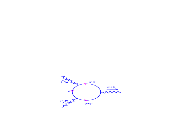
In order to evaluate the first nonvanishing contribution, let us take $n=2$ in the one-loop contribution (2.8), which is shown in Fig.Β 1:

ΞžΞΌβ€‹Ξ½β€‹(p)=∫d3​q(2​π)3​t​r​[(qΜΈ+pΜΈ+m)​γμ​(qΜΈ+m)​γν][(q+p)2βˆ’m2]​[q2βˆ’m2].superscriptΞžπœ‡πœˆπ‘superscript𝑑3π‘žsuperscript2πœ‹3π‘‘π‘Ÿdelimited-[]italic-qΜΈitalic-pΜΈπ‘šsuperscriptπ›Ύπœ‡italic-qΜΈπ‘šsuperscriptπ›Ύπœˆdelimited-[]superscriptπ‘žπ‘2superscriptπ‘š2delimited-[]superscriptπ‘ž2superscriptπ‘š2\Xi^{\mu\nu}\left(p\right)=\int\frac{d^{3}q}{\left(2\pi\right)^{3}}\frac{tr\left[\left(\displaystyle{\not}q+\displaystyle{\not}p+m\right)\gamma^{\mu}\left(\displaystyle{\not}q+m\right)\gamma^{\nu}\right]}{\left[\left(q+p\right)^{2}-m^{2}\right]\left[q^{2}-m^{2}\right]}. (3.1)

This expression can be put into a more convenient form, which facilitates the evaluation of the momentum integration. Thus, we can make use of the Feynman parametrization, which combined with the change of variables $q\rightarrow q+xp$ results into

ΞžΞΌβ€‹Ξ½β€‹(p)=∫01𝑑xβ€‹βˆ«d3​q(2​π)3​t​r​[(qΜΈ+(1βˆ’x)​pΜΈ+m)​γμ​(qΜΈβˆ’x​pΜΈ+m)​γν][q2+x​(1βˆ’x)​p2βˆ’m2]2.superscriptΞžπœ‡πœˆπ‘superscriptsubscript01differential-dπ‘₯superscript𝑑3π‘žsuperscript2πœ‹3π‘‘π‘Ÿdelimited-[]italic-qΜΈ1π‘₯italic-pΜΈπ‘šsuperscriptπ›Ύπœ‡italic-qΜΈπ‘₯italic-pΜΈπ‘šsuperscriptπ›Ύπœˆsuperscriptdelimited-[]superscriptπ‘ž2π‘₯1π‘₯superscript𝑝2superscriptπ‘š22\Xi^{\mu\nu}\left(p\right)=\int_{0}^{1}dx\int\frac{d^{3}q}{\left(2\pi\right)^{3}}\frac{tr\left[\left(\displaystyle{\not}q+\left(1-x\right)\displaystyle{\not}p+m\right)\gamma^{\mu}\left(\displaystyle{\not}q-x\displaystyle{\not}p+m\right)\gamma^{\nu}\right]}{\left[q^{2}+x\left(1-x\right)p^{2}-m^{2}\right]^{2}}. (3.2)

We can evaluate the trace in (3.2) and write the integration into a dimensional regularization form. Hence, with the known results for a two-dimensional representation,

$$tr\left(\gamma^{\mu}\gamma^{\nu}\right)=2\eta^{\mu\nu},\quad tr\left(\gamma^{\mu}\gamma^{\beta}\gamma^{\nu}\right)=2i\epsilon^{\mu\beta\nu},\quad tr\left(\gamma^{\alpha}\gamma^{\mu}\gamma^{\beta}\gamma^{\nu}\right)=2\left(\eta^{\alpha\mu}\eta^{\beta\nu}-\eta^{\alpha\beta}\eta^{\mu\nu}+\eta^{\alpha\nu}\eta^{\mu\beta}\right),$$ (3.3)

we obtain [26]

$$\Xi^{\mu\nu}\left(p\right)=2\int_{0}^{1}dx\int\frac{d^{d}q}{\left(2\pi\right)^{d}}\frac{\left(\frac{2}{d}-1\right)q^{2}\eta^{\mu\nu}-2x\left(1-x\right)p^{\mu}p^{\nu}+imp_{\alpha}\epsilon^{\alpha\mu\nu}+\left(m^{2}+x\left(1-x\right)p^{2}\right)\eta^{\mu\nu}}{\left[q^{2}+x\left(1-x\right)p^{2}-m^{2}\right]^{2}}.$$ (3.4)

Here $d$ denotes the dimension of the space-time. The detailed evaluation of the momentum integral is rather direct, taking the limit $d\rightarrow 3$ and the resulting expression reads

$\displaystyle\Xi^{\mu\nu}\left(p\right)$ $\displaystyle=-\frac{1}{4\pi}mp_{\alpha}\epsilon^{\alpha\mu\nu}\int_{0}^{1}dx\frac{1}{\left(m^{2}-x\left(1-x\right)p^{2}\right)^{\frac{1}{2}}}+\frac{i}{2\pi}\left(p^{2}\eta^{\mu\nu}-p^{\mu}p^{\nu}\right)\int_{0}^{1}dx\frac{x\left(1-x\right)}{\left(m^{2}-x\left(1-x\right)p^{2}\right)^{\frac{1}{2}}}.$ (3.5)

3.1.1 Higher derivative contribution

Let us take a closer look at the expression (3.5). The higher-derivative contributions are obtained by considering the long wavelength limit $p^{2}\ll m^{2}$. Thus expanding the expression and performing the remaining integrals, we obtain

$\displaystyle\Xi^{\mu\nu}\left(p\right)$ =βˆ’s​g​n​(m)4​π​(pα​ϡα​μ​ν)​(1+p212​m2)+i12​π​1|m|​(p2β€‹Ξ·ΞΌβ€‹Ξ½βˆ’pμ​pΞ½)+π’ͺ​(p4m4),absentπ‘ π‘”π‘›π‘š4πœ‹subscript𝑝𝛼superscriptitalic-Ο΅π›Όπœ‡πœˆ1superscript𝑝212superscriptπ‘š2𝑖12πœ‹1π‘šsuperscript𝑝2superscriptπœ‚πœ‡πœˆsuperscriptπ‘πœ‡superscriptπ‘πœˆπ’ͺsuperscript𝑝4superscriptπ‘š4\displaystyle=-\frac{sgn\left(m\right)}{4\pi}\left(p_{\alpha}\epsilon^{\alpha\mu\nu}\right)\left(1+\frac{p^{2}}{12m^{2}}\right)+\frac{i}{12\pi}\frac{1}{\left|m\right|}\left(p^{2}\eta^{\mu\nu}-p^{\mu}p^{\nu}\right)+\mathcal{O}\left(\frac{p^{4}}{m^{4}}\right), (3.6)

in which, s​g​n​(m)≑m|m|π‘ π‘”π‘›π‘šπ‘šπ‘šsgn\left(m\right)\equiv\frac{m}{\left|m\right|} is the sign function. As it is easily seen, the first term corresponds to the kinetic term of the Chern-Simons term, $\mathcal{O}\left(m^{0}\right)$, and its HD extension, $\mathcal{O}\left(m^{-2}\right)$, while the second one is the kinetic part of the noncommutative Maxwell action, $\mathcal{O}\left(m^{-1}\right)$. By means of illustration, let us consider the first term from (3.6) which corresponds to the Chern-Simons contribution

$\displaystyle\Xi_{\tiny\mbox{CS}}^{\mu\nu}\left(p\right)$ =βˆ’s​g​n​(m)4​π​(pα​ϡα​μ​ν)​(1+p212​m2+π’ͺ​(p4m4)).absentπ‘ π‘”π‘›π‘š4πœ‹subscript𝑝𝛼superscriptitalic-Ο΅π›Όπœ‡πœˆ1superscript𝑝212superscriptπ‘š2π’ͺsuperscript𝑝4superscriptπ‘š4\displaystyle=-\frac{sgn\left(m\right)}{4\pi}\left(p_{\alpha}\epsilon^{\alpha\mu\nu}\right)\left(1+\frac{p^{2}}{12m^{2}}+\mathcal{O}\left(\frac{p^{4}}{m^{4}}\right)\right). (3.7)

Substituting it into the expression (2.7) and after some integral manipulation, we find

$\displaystyle\Gamma_{\tiny\mbox{CS}}^{\mu\nu}\left(x_{1},x_{2}\right)$ $\displaystyle=-\frac{g^{2}}{2}\int\frac{d^{3}p}{\left(2\pi\right)^{3}}\exp\left[-ip.\left(x_{1}-x_{2}\right)\right]\Xi_{cs}^{\mu\nu}\left(p\right),$
=βˆ’i​g28​π​s​g​n​(m)​ϡα​μ​ν​(1βˆ’β–‘12​m2)β€‹βˆ‚Ξ±Ξ΄β€‹(x1βˆ’x2).absent𝑖superscript𝑔28πœ‹π‘ π‘”π‘›π‘šsuperscriptitalic-Ο΅π›Όπœ‡πœˆ1β–‘12superscriptπ‘š2subscript𝛼𝛿subscriptπ‘₯1subscriptπ‘₯2\displaystyle=-i\frac{g^{2}}{8\pi}sgn\left(m\right)\epsilon^{\alpha\mu\nu}\left(1-\frac{\square}{12m^{2}}\right)\partial_{\alpha}\delta\left(x_{1}-x_{2}\right). (3.8)

Finally, we substitute (3.8) into (2.6) to then obtain the expression for the Chern-Simons effective action

$\displaystyle i\Gamma_{\tiny\mbox{CS}}\left[AA\right]$ =i​g28​π​s​g​n​(m)β€‹Ο΅ΞΌβ€‹Ξ±β€‹Ξ½β€‹βˆ«d3​x​[Aμ​(x)​(1βˆ’β–‘12​m2)β€‹βˆ‚Ξ±Aν​(x)].absent𝑖superscript𝑔28πœ‹π‘ π‘”π‘›π‘šsuperscriptitalic-Ο΅πœ‡π›Όπœˆsuperscript𝑑3π‘₯delimited-[]subscriptπ΄πœ‡π‘₯1β–‘12superscriptπ‘š2subscript𝛼subscript𝐴𝜈π‘₯\displaystyle=i\frac{g^{2}}{8\pi}sgn\left(m\right)\epsilon^{\mu\alpha\nu}\int d^{3}x\left[A_{\mu}\left(x\right)\left(1-\frac{\square}{12m^{2}}\right)\partial_{\alpha}A_{\nu}\left(x\right)\right]. (3.9)

As it is well known, the expression for two gauge fields (3.9) does not display effects from noncommutativity, since the phase factor from (2.7) vanishes for $n=2$. Furthermore, one can perform the same manipulation as above and realize that the second term in (3.6), when written in terms of the effective action, is the quadratic part of the noncommutative Maxwell action

$\displaystyle i\Gamma_{\tiny\mbox{M}}\left[AA\right]$ $\displaystyle=i\frac{g^{2}}{24\pi}\frac{1}{\left|m\right|}\int d^{3}x\left[\partial^{\nu}A_{\mu}\partial_{\nu}A^{\mu}-\partial^{\nu}A_{\mu}\partial^{\mu}A_{\nu}\right].$ (3.10)

3.2 AAA-term contribution

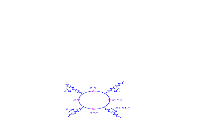
In the same way as the previous calculation, we start by evaluating the one-loop contribution (2.8) for the case $n=3$, represented in Fig.Β 2:

ΞžΞΌβ€‹Ξ½β€‹Οƒβ€‹(p,k)=∫d3​q(2​π)3​t​r​[(qΜΈ+pΜΈ+m)​γμ​(qΜΈ+m)​γν​(qΜΈβˆ’kΜΈ+m)​γσ][(q+p)2βˆ’m2]​[q2βˆ’m2]​[(qβˆ’k)2βˆ’m2].superscriptΞžπœ‡πœˆπœŽπ‘π‘˜superscript𝑑3π‘žsuperscript2πœ‹3π‘‘π‘Ÿdelimited-[]italic-qΜΈitalic-pΜΈπ‘šsuperscriptπ›Ύπœ‡italic-qΜΈπ‘šsuperscriptπ›Ύπœˆitalic-qΜΈitalic-kΜΈπ‘šsuperscriptπ›ΎπœŽdelimited-[]superscriptπ‘žπ‘2superscriptπ‘š2delimited-[]superscriptπ‘ž2superscriptπ‘š2delimited-[]superscriptπ‘žπ‘˜2superscriptπ‘š2\Xi^{\mu\nu\sigma}\left(p,k\right)=\int\frac{d^{3}q}{\left(2\pi\right)^{3}}\frac{tr\left[\left(\displaystyle{\not}q+\displaystyle{\not}p+m\right)\gamma^{\mu}\left(\displaystyle{\not}q+m\right)\gamma^{\nu}\left(\displaystyle{\not}q-\displaystyle{\not}k+m\right)\gamma^{\sigma}\right]}{\left[\left(q+p\right)^{2}-m^{2}\right]\left[q^{2}-m^{2}\right]\left[\left(q-k\right)^{2}-m^{2}\right]}. (3.11)

Moreover, we can use the Feynman parametrization and the change of variables qβ†’qβˆ’(x​pβˆ’z​k)≑qβˆ’sβ†’π‘žπ‘žπ‘₯π‘π‘§π‘˜π‘žπ‘ q\rightarrow q-\left(xp-zk\right)\equiv q-s to obtain

ΞžΞΌβ€‹Ξ½β€‹Οƒβ€‹(p,k)=2β€‹βˆ«π‘‘ΞΎβ€‹βˆ«d3​q(2​π)3​t​r​[(qΜΈβˆ’sΜΈ+pΜΈ+m)​γμ​(qΜΈβˆ’sΜΈ+m)​γν​(qΜΈβˆ’sΜΈβˆ’kΜΈ+m)​γσ][q2+A2​(p,k)βˆ’m2]3,superscriptΞžπœ‡πœˆπœŽπ‘π‘˜2differential-dπœ‰superscript𝑑3π‘žsuperscript2πœ‹3π‘‘π‘Ÿdelimited-[]italic-qΜΈitalic-sΜΈitalic-pΜΈπ‘šsuperscriptπ›Ύπœ‡italic-qΜΈitalic-sΜΈπ‘šsuperscriptπ›Ύπœˆitalic-qΜΈitalic-sΜΈitalic-kΜΈπ‘šsuperscriptπ›ΎπœŽsuperscriptdelimited-[]superscriptπ‘ž2superscript𝐴2π‘π‘˜superscriptπ‘š23\Xi^{\mu\nu\sigma}\left(p,k\right)=2\int d\xi\int\frac{d^{3}q}{\left(2\pi\right)^{3}}\frac{tr\left[\left(\displaystyle{\not}q-\displaystyle{\not}s+\displaystyle{\not}p+m\right)\gamma^{\mu}\left(\displaystyle{\not}q-\displaystyle{\not}s+m\right)\gamma^{\nu}\left(\displaystyle{\not}q-\displaystyle{\not}s-\displaystyle{\not}k+m\right)\gamma^{\sigma}\right]}{\left[q^{2}+A^{2}\left(p,k\right)-m^{2}\right]^{3}}, (3.12)
Refer to caption
Figure 2: Relevant graph for the AAA-term.

where we have introduced the notation $\int d\xi=\int_{0}^{1}dx\int_{0}^{1-x}dz$, and $A^{2}\left(p,k\right)=-\left(xp-zk\right)^{2}+xp^{2}+zk^{2}$. The momentum integration can be performed without any complication by using standard methods. Hence, after separating the different powers of $q$ in the numerator and then evaluating the integration, we find

$\displaystyle\Xi^{\mu\nu\sigma}\left(p,k\right)$ $\displaystyle=\frac{i}{16\pi}\int d\xi\left[\frac{A^{\mu\nu\sigma}\left(p,k;x,z\right)}{\left(m^{2}-A^{2}\left(p,k\right)\right)^{\frac{1}{2}}}-\frac{B^{\mu\nu\sigma}\left(p,k;x,z\right)}{\left(m^{2}-A^{2}\left(p,k\right)\right)^{\frac{3}{2}}}\right],$ (3.13)

by sake of notation, we have introduced the quantities, with sΞΌ=x​pΞΌβˆ’z​kΞΌsubscriptπ‘ πœ‡π‘₯subscriptπ‘πœ‡π‘§subscriptπ‘˜πœ‡s_{\mu}=xp_{\mu}-zk_{\mu},

Aμ​ν​σ​(p,k;x,z)=superscriptπ΄πœ‡πœˆπœŽπ‘π‘˜π‘₯𝑧absent\displaystyle A^{\mu\nu\sigma}\left(p,k;x,z\right)= t​r​[γα​γμ​γα​γν​(βˆ’sΜΈβˆ’kΜΈ+m)​γσ]βˆ’t​r​[γα​γμ​s̸​γν​γα​γσ]π‘‘π‘Ÿdelimited-[]superscript𝛾𝛼superscriptπ›Ύπœ‡subscript𝛾𝛼superscriptπ›Ύπœˆitalic-sΜΈitalic-kΜΈπ‘šsuperscriptπ›ΎπœŽπ‘‘π‘Ÿdelimited-[]superscript𝛾𝛼superscriptπ›Ύπœ‡italic-sΜΈsuperscriptπ›Ύπœˆsubscript𝛾𝛼superscriptπ›ΎπœŽ\displaystyle tr\left[\gamma^{\alpha}\gamma^{\mu}\gamma_{\alpha}\gamma^{\nu}\left(-\displaystyle{\not}s-\displaystyle{\not}k+m\right)\gamma^{\sigma}\right]-tr\left[\gamma^{\alpha}\gamma^{\mu}\displaystyle{\not}s\gamma^{\nu}\gamma_{\alpha}\gamma^{\sigma}\right]
+m​t​r​[γα​γμ​γν​γα​γσ]βˆ’t​r​[s̸​γμ​γα​γν​γα​γσ]π‘šπ‘‘π‘Ÿdelimited-[]superscript𝛾𝛼superscriptπ›Ύπœ‡superscriptπ›Ύπœˆsubscript𝛾𝛼superscriptπ›ΎπœŽπ‘‘π‘Ÿdelimited-[]italic-sΜΈsuperscriptπ›Ύπœ‡superscript𝛾𝛼superscriptπ›Ύπœˆsubscript𝛾𝛼superscriptπ›ΎπœŽ\displaystyle+mtr\left[\gamma^{\alpha}\gamma^{\mu}\gamma^{\nu}\gamma_{\alpha}\gamma^{\sigma}\right]-tr\left[\displaystyle{\not}s\gamma^{\mu}\gamma^{\alpha}\gamma^{\nu}\gamma_{\alpha}\gamma^{\sigma}\right]
+t​r​[p̸​γμ​γα​γν​γα​γσ]+m​t​r​[γμ​γα​γν​γα​γσ],π‘‘π‘Ÿdelimited-[]italic-pΜΈsuperscriptπ›Ύπœ‡superscript𝛾𝛼superscriptπ›Ύπœˆsubscript𝛾𝛼superscriptπ›ΎπœŽπ‘šπ‘‘π‘Ÿdelimited-[]superscriptπ›Ύπœ‡superscript𝛾𝛼superscriptπ›Ύπœˆsubscript𝛾𝛼superscriptπ›ΎπœŽ\displaystyle+tr\left[\displaystyle{\not}p\gamma^{\mu}\gamma^{\alpha}\gamma^{\nu}\gamma_{\alpha}\gamma^{\sigma}\right]+mtr\left[\gamma^{\mu}\gamma^{\alpha}\gamma^{\nu}\gamma_{\alpha}\gamma^{\sigma}\right], (3.14)

and

Bμ​ν​σ​(p,k;x,z)=superscriptπ΅πœ‡πœˆπœŽπ‘π‘˜π‘₯𝑧absent\displaystyle B^{\mu\nu\sigma}\left(p,k;x,z\right)= t​r​[s̸​γμ​s̸​γν​(βˆ’sΜΈβˆ’kΜΈ+m)​γσ]βˆ’m​t​r​[s̸​γμ​γν​(βˆ’sΜΈβˆ’kΜΈ+m)​γσ]π‘‘π‘Ÿdelimited-[]italic-sΜΈsuperscriptπ›Ύπœ‡italic-sΜΈsuperscriptπ›Ύπœˆitalic-sΜΈitalic-kΜΈπ‘šsuperscriptπ›ΎπœŽπ‘šπ‘‘π‘Ÿdelimited-[]italic-sΜΈsuperscriptπ›Ύπœ‡superscriptπ›Ύπœˆitalic-sΜΈitalic-kΜΈπ‘šsuperscriptπ›ΎπœŽ\displaystyle tr\left[\displaystyle{\not}s\gamma^{\mu}\displaystyle{\not}s\gamma^{\nu}\left(-\displaystyle{\not}s-\displaystyle{\not}k+m\right)\gamma^{\sigma}\right]-mtr\left[\displaystyle{\not}s\gamma^{\mu}\gamma^{\nu}\left(-\displaystyle{\not}s-\displaystyle{\not}k+m\right)\gamma^{\sigma}\right]
βˆ’t​r​[p̸​γμ​s̸​γν​(βˆ’sΜΈβˆ’kΜΈ+m)​γσ]+m​t​r​[p̸​γμ​γν​(βˆ’sΜΈβˆ’kΜΈ+m)​γσ]π‘‘π‘Ÿdelimited-[]italic-pΜΈsuperscriptπ›Ύπœ‡italic-sΜΈsuperscriptπ›Ύπœˆitalic-sΜΈitalic-kΜΈπ‘šsuperscriptπ›ΎπœŽπ‘šπ‘‘π‘Ÿdelimited-[]italic-pΜΈsuperscriptπ›Ύπœ‡superscriptπ›Ύπœˆitalic-sΜΈitalic-kΜΈπ‘šsuperscriptπ›ΎπœŽ\displaystyle-tr\left[\displaystyle{\not}p\gamma^{\mu}\displaystyle{\not}s\gamma^{\nu}\left(-\displaystyle{\not}s-\displaystyle{\not}k+m\right)\gamma^{\sigma}\right]+mtr\left[\displaystyle{\not}p\gamma^{\mu}\gamma^{\nu}\left(-\displaystyle{\not}s-\displaystyle{\not}k+m\right)\gamma^{\sigma}\right]
βˆ’m​t​r​[γμ​s̸​γν​(βˆ’sΜΈβˆ’kΜΈ+m)​γσ]+m2​t​r​[γμ​γν​(βˆ’sΜΈβˆ’kΜΈ+m)​γσ].π‘šπ‘‘π‘Ÿdelimited-[]superscriptπ›Ύπœ‡italic-sΜΈsuperscriptπ›Ύπœˆitalic-sΜΈitalic-kΜΈπ‘šsuperscriptπ›ΎπœŽsuperscriptπ‘š2π‘‘π‘Ÿdelimited-[]superscriptπ›Ύπœ‡superscriptπ›Ύπœˆitalic-sΜΈitalic-kΜΈπ‘šsuperscriptπ›ΎπœŽ\displaystyle-mtr\left[\gamma^{\mu}\displaystyle{\not}s\gamma^{\nu}\left(-\displaystyle{\not}s-\displaystyle{\not}k+m\right)\gamma^{\sigma}\right]+m^{2}tr\left[\gamma^{\mu}\gamma^{\nu}\left(-\displaystyle{\not}s-\displaystyle{\not}k+m\right)\gamma^{\sigma}\right]. (3.15)

As usual, we could analyze in detail the full contribution of (3.13), but since we are interested in particular cases that induce the $AAA$ noncommutative parts of the Chern-Simons and Maxwell action, we will retain our attention into the $\mathcal{O}\left(m^{0}\right)$, $\mathcal{O}\left(m^{-1}\right)$ and $\mathcal{O}\left(m^{-2}\right)$ contributions.

3.2.1 Higher derivative contribution

The contributions for the effective action from $AAA$ gauge fields are more complicated than those from the $AA$ fields; this is due to the structure of the denominator and numerator of the terms from the expression (3.13). Nevertheless, the contributions for the Chern-Simons action and its HD extension are those associated with terms of order $\mathcal{O}\left(m^{0}\right)$ and $\mathcal{O}\left(m^{-2}\right)$. Hence, by simple power counting, we consider those terms that are linear in $m$ from (3.14),

$\displaystyle A_{\tiny\mbox{CS}}^{\mu\nu\sigma}$ $\displaystyle\left(p,k;x,z\right)=-mtr\left[\gamma^{\mu}\gamma^{\nu}\gamma^{\sigma}\right]-mtr\left[\gamma^{\mu}\gamma^{\nu}\gamma^{\sigma}\right]-mtr\left[\gamma^{\mu}\gamma^{\nu}\gamma^{\sigma}\right],$ (3.16)

and those that are linear and cubic in $m$ from (3.15),

BCSμ​ν​σ​(p,k;x,z)superscriptsubscript𝐡CSπœ‡πœˆπœŽπ‘π‘˜π‘₯𝑧\displaystyle B_{\tiny\mbox{CS}}^{\mu\nu\sigma}\left(p,k;x,z\right) =m​t​r​[(sΜΈβˆ’pΜΈ)​γμ​s̸​γν​γσ]+m​t​r​[(sΜΈβˆ’pΜΈ)​γμ​γν​(sΜΈ+kΜΈ)​γσ]absentπ‘šπ‘‘π‘Ÿdelimited-[]italic-sΜΈitalic-pΜΈsuperscriptπ›Ύπœ‡italic-sΜΈsuperscriptπ›Ύπœˆsuperscriptπ›ΎπœŽπ‘šπ‘‘π‘Ÿdelimited-[]italic-sΜΈitalic-pΜΈsuperscriptπ›Ύπœ‡superscriptπ›Ύπœˆitalic-sΜΈitalic-kΜΈsuperscriptπ›ΎπœŽ\displaystyle=mtr\left[\left(\displaystyle{\not}s-\displaystyle{\not}p\right)\gamma^{\mu}\displaystyle{\not}s\gamma^{\nu}\gamma^{\sigma}\right]+mtr\left[\left(\displaystyle{\not}s-\displaystyle{\not}p\right)\gamma^{\mu}\gamma^{\nu}\left(\displaystyle{\not}s+\displaystyle{\not}k\right)\gamma^{\sigma}\right]
+m​t​r​[γμ​s̸​γν​(sΜΈ+kΜΈ)​γσ]+m3​t​r​[γμ​γν​γσ],π‘šπ‘‘π‘Ÿdelimited-[]superscriptπ›Ύπœ‡italic-sΜΈsuperscriptπ›Ύπœˆitalic-sΜΈitalic-kΜΈsuperscriptπ›ΎπœŽsuperscriptπ‘š3π‘‘π‘Ÿdelimited-[]superscriptπ›Ύπœ‡superscriptπ›Ύπœˆsuperscriptπ›ΎπœŽ\displaystyle+mtr\left[\gamma^{\mu}\displaystyle{\not}s\gamma^{\nu}\left(\displaystyle{\not}s+\displaystyle{\not}k\right)\gamma^{\sigma}\right]+m^{3}tr\left[\gamma^{\mu}\gamma^{\nu}\gamma^{\sigma}\right], (3.17)

while, for the Maxwell action we shall consider the terms $\mathcal{O}\left(m^{-1}\right)$, which are those terms independent of $m$ in (3.14),

AMμ​ν​σ​(p,k;x,z)superscriptsubscript𝐴Mπœ‡πœˆπœŽπ‘π‘˜π‘₯𝑧\displaystyle A_{\tiny\mbox{M}}^{\mu\nu\sigma}\left(p,k;x,z\right) =t​r​[γμ​γν​(sΜΈ+kΜΈ)​γσ]+t​r​[γμ​s̸​γν​γσ]+t​r​[s̸​γμ​γν​γσ]βˆ’t​r​[p̸​γμ​γν​γσ],absentπ‘‘π‘Ÿdelimited-[]superscriptπ›Ύπœ‡superscriptπ›Ύπœˆitalic-sΜΈitalic-kΜΈsuperscriptπ›ΎπœŽπ‘‘π‘Ÿdelimited-[]superscriptπ›Ύπœ‡italic-sΜΈsuperscriptπ›Ύπœˆsuperscriptπ›ΎπœŽπ‘‘π‘Ÿdelimited-[]italic-sΜΈsuperscriptπ›Ύπœ‡superscriptπ›Ύπœˆsuperscriptπ›ΎπœŽπ‘‘π‘Ÿdelimited-[]italic-pΜΈsuperscriptπ›Ύπœ‡superscriptπ›Ύπœˆsuperscriptπ›ΎπœŽ\displaystyle=tr\left[\gamma^{\mu}\gamma^{\nu}\left(\displaystyle{\not}s+\displaystyle{\not}k\right)\gamma^{\sigma}\right]+tr\left[\gamma^{\mu}\displaystyle{\not}s\gamma^{\nu}\gamma^{\sigma}\right]+tr\left[\displaystyle{\not}s\gamma^{\mu}\gamma^{\nu}\gamma^{\sigma}\right]-tr\left[\displaystyle{\not}p\gamma^{\mu}\gamma^{\nu}\gamma^{\sigma}\right], (3.18)

and quadratic in $m$ from (3.15),

BMμ​ν​σ​(p,k;x,z)superscriptsubscript𝐡Mπœ‡πœˆπœŽπ‘π‘˜π‘₯𝑧\displaystyle B_{\tiny\mbox{M}}^{\mu\nu\sigma}\left(p,k;x,z\right) =βˆ’m2​t​r​[s̸​γμ​γν​γσ]+m2​t​r​[p̸​γμ​γν​γσ]absentsuperscriptπ‘š2π‘‘π‘Ÿdelimited-[]italic-sΜΈsuperscriptπ›Ύπœ‡superscriptπ›Ύπœˆsuperscriptπ›ΎπœŽsuperscriptπ‘š2π‘‘π‘Ÿdelimited-[]italic-pΜΈsuperscriptπ›Ύπœ‡superscriptπ›Ύπœˆsuperscriptπ›ΎπœŽ\displaystyle=-m^{2}tr\left[\displaystyle{\not}s\gamma^{\mu}\gamma^{\nu}\gamma^{\sigma}\right]+m^{2}tr\left[\displaystyle{\not}p\gamma^{\mu}\gamma^{\nu}\gamma^{\sigma}\right]
βˆ’m2​t​r​[γμ​s̸​γν​γσ]βˆ’m2​t​r​[γμ​γν​(sΜΈ+kΜΈ)​γσ].superscriptπ‘š2π‘‘π‘Ÿdelimited-[]superscriptπ›Ύπœ‡italic-sΜΈsuperscriptπ›Ύπœˆsuperscriptπ›ΎπœŽsuperscriptπ‘š2π‘‘π‘Ÿdelimited-[]superscriptπ›Ύπœ‡superscriptπ›Ύπœˆitalic-sΜΈitalic-kΜΈsuperscriptπ›ΎπœŽ\displaystyle-m^{2}tr\left[\gamma^{\mu}\displaystyle{\not}s\gamma^{\nu}\gamma^{\sigma}\right]-m^{2}tr\left[\gamma^{\mu}\gamma^{\nu}\left(\displaystyle{\not}s+\displaystyle{\not}k\right)\gamma^{\sigma}\right]. (3.19)

Let us now focus our attention into the Chern-Simons contributions. We can simplify the above equations by means of the Clifford algebra $\left\{\gamma^{\mu},\gamma^{\nu}\right\}=2\eta^{\mu\nu}$ and the identities (3.3), resulting in the following expressions

$\displaystyle A_{\tiny\mbox{CS}}^{\mu\nu\sigma}\left(p,k;x,z\right)$ $\displaystyle=-6im\epsilon^{\mu\nu\sigma},$ (3.20)

and

$\displaystyle B_{\tiny\mbox{CS}}^{\mu\nu\sigma}\left(p,k;x,z\right)$ $\displaystyle=im\widetilde{B}_{\tiny\mbox{CS}}^{\mu\nu\sigma}\left(p,k;x,z\right)+2im^{3}\epsilon^{\mu\nu\sigma},$ (3.21)

where we have defined the quantity

$\displaystyle\widetilde{B}_{\tiny\mbox{CS}}^{\mu\nu\sigma}\left(p,k;x,z\right)$ =2​(pμ​kΞ±βˆ’sμ​sΞ±βˆ’2​sμ​kΞ±)​ϡα​ν​σ+2​(sα​sΞ½βˆ’2​sν​pΞ±βˆ’pα​kΞ½)​ϡα​μ​σabsent2superscriptπ‘πœ‡subscriptπ‘˜π›Όsuperscriptπ‘ πœ‡subscript𝑠𝛼2superscriptπ‘ πœ‡subscriptπ‘˜π›Όsuperscriptitalic-Ο΅π›ΌπœˆπœŽ2subscript𝑠𝛼superscriptπ‘ πœˆ2superscriptπ‘ πœˆsubscript𝑝𝛼subscript𝑝𝛼superscriptπ‘˜πœˆsuperscriptitalic-Ο΅π›Όπœ‡πœŽ\displaystyle=2\left(p^{\mu}k_{\alpha}-s^{\mu}s_{\alpha}-2s^{\mu}k_{\alpha}\right)\epsilon^{\alpha\nu\sigma}+2\left(s_{\alpha}s^{\nu}-2s^{\nu}p_{\alpha}-p_{\alpha}k^{\nu}\right)\epsilon^{\alpha\mu\sigma}
βˆ’2​(sα​sΟƒ+2​pα​kΟƒ)​ϡα​μ​ν+2​pα​kβ​ην​σ​ϡα​μ​β.2subscript𝑠𝛼superscriptπ‘ πœŽ2subscript𝑝𝛼superscriptπ‘˜πœŽsuperscriptitalic-Ο΅π›Όπœ‡πœˆ2subscript𝑝𝛼subscriptπ‘˜π›½superscriptπœ‚πœˆπœŽsuperscriptitalic-Ο΅π›Όπœ‡π›½\displaystyle-2\left(s_{\alpha}s^{\sigma}+2p_{\alpha}k^{\sigma}\right)\epsilon^{\alpha\mu\nu}+2p_{\alpha}k_{\beta}\eta^{\nu\sigma}\epsilon^{\alpha\mu\beta}. (3.22)

Hence, replacing the expressions (3.20) and (3.21) back into (3.13), we find the following expression for the Chern-Simons contribution:

$\displaystyle\Xi_{\tiny\mbox{CS}}^{\mu\nu\sigma}\left(p,k\right)$ =12​π​s​g​n​(m)β€‹βˆ«π‘‘ΞΎβ€‹[ϡμ​ν​σ+18​m2​(6​ϡμ​ν​σ​A2​(p,k)+B~CSμ​ν​σ​(p,k;x,z))].absent12πœ‹π‘ π‘”π‘›π‘šdifferential-dπœ‰delimited-[]superscriptitalic-Ο΅πœ‡πœˆπœŽ18superscriptπ‘š26superscriptitalic-Ο΅πœ‡πœˆπœŽsuperscript𝐴2π‘π‘˜superscriptsubscript~𝐡CSπœ‡πœˆπœŽπ‘π‘˜π‘₯𝑧\displaystyle=\frac{1}{2\pi}sgn\left(m\right)\int d\xi\left[\epsilon^{\mu\nu\sigma}+\frac{1}{8m^{2}}\bigg{(}6\epsilon^{\mu\nu\sigma}A^{2}\left(p,k\right)+\widetilde{B}_{\tiny\mbox{CS}}^{\mu\nu\sigma}\left(p,k;x,z\right)\bigg{)}\right]. (3.23)

From the expression (3.23) we see that, differently from the contributions appearing in the $AA$-term, (3.7), we now have HD terms with different indices in the antisymmetric Levi-CivitΓ  tensor, this shows that these HD terms arising from $\widetilde{B}_{\tiny\mbox{CS}}^{\mu\nu\sigma}$ contribute in a more involving form in terms of derivatives than those arising from $\epsilon^{\mu\nu\sigma}A^{2}$. Nonetheless, the remaining integrals in (3.23) can be readily evaluated to give

$\displaystyle\int d\xi A^{2}\left(p,k\right)$ $\displaystyle=\frac{1}{12}\left(p^{2}+\left(p.k\right)+k^{2}\right),$ (3.24)

and

$\displaystyle\int d\xi\widetilde{B}_{\tiny\mbox{CS}}^{\mu\nu\sigma}$ $\displaystyle=\frac{1}{6}\bigg{[}\epsilon^{\alpha\nu\sigma}(\frac{5}{2}p^{\mu}k_{\alpha}-p^{\mu}p_{\alpha}+\frac{1}{2}k^{\mu}p_{\alpha}+3k^{\mu}k_{\alpha})+\epsilon^{\alpha\mu\sigma}(-3p_{\alpha}p^{\nu}-k_{\alpha}p^{\nu}+k_{\alpha}k^{\nu}-3p_{\alpha}k^{\nu})$
$\displaystyle-\epsilon^{\alpha\mu\nu}(p_{\alpha}p^{\sigma}-k_{\alpha}p^{\sigma}+k_{\alpha}k^{\sigma}+5p_{\alpha}k^{\sigma})\bigg{]}+\epsilon^{\alpha\mu\beta}\eta^{\nu\sigma}p_{\alpha}k_{\beta}.$ (3.25)

Finally, to obtain the second part of the Chern-Simons and its HD extension contributions to the effective action, we should replace the above results in such a way: first (3.24) and (3.25) into (3.23), and then substituting the resulting expression back into (2.6) (for the case $n=3$), with the choice $p_{1}=p$ and $p_{2}=k$ then $p_{3}=-p-k$, after such substitution we get

$\displaystyle i\Gamma_{\tiny\mbox{CS}}[AAA]$ $\displaystyle=\frac{g^{3}}{3}\int d^{3}x_{1}d^{3}x_{2}d^{3}x_{3}~{}A_{\mu}(x_{1})A_{\nu}(x_{2})A_{\sigma}(x_{3})$
$\displaystyle\times\int\frac{d^{3}p}{(2\pi)^{3}}\frac{d^{3}k}{(2\pi)^{3}}\exp[-ip.(x_{1}-x_{3})-ik.(x_{2}-x_{3})]\exp[-\frac{i}{2}(p\times k)]~{}\Xi_{\tiny\mbox{CS}}^{\mu\nu\sigma}.$ (3.26)

Thus, after some manipulation involving the momentum factors becoming derivatives, and integrations involving the noncommutativity between the gauge fields, we are able to find the final expression for the Chern-Simons effective action for the $AAA$-gauge fields,

$\displaystyle i\Gamma_{\tiny\mbox{CS}}[AAA]$ =g312​π​s​g​n​(m)β€‹βˆ«d3​x​Ρμ​ν​σ​Aμ⋆Aν⋆AΟƒabsentsuperscript𝑔312πœ‹π‘ π‘”π‘›π‘šβ‹†superscript𝑑3π‘₯superscriptπœ€πœ‡πœˆπœŽsubscriptπ΄πœ‡subscript𝐴𝜈subscript𝐴𝜎\displaystyle=\frac{g^{3}}{12\pi}~{}sgn(m)\int d^{3}x~{}\varepsilon^{\mu\nu\sigma}A_{\mu}\star A_{\nu}\star A_{\sigma}
$\displaystyle-\frac{g^{3}}{48\pi m^{2}}~{}sgn(m)\int d^{3}x~{}\bigg{\{}\frac{3}{4}~{}\varepsilon^{\mu\nu\sigma}\Box A_{\mu}\star A_{\nu}\star A_{\sigma}+\varepsilon^{\alpha\mu\beta}\eta^{\nu\sigma}\partial_{\alpha}A_{\mu}\star\partial_{\beta}A_{\nu}\star A_{\sigma}$
$\displaystyle+\frac{1}{12}\varepsilon^{\alpha\nu\sigma}\bigg{[}13\partial_{\alpha}A_{\sigma}\star\partial^{\mu}A_{\nu}\star A_{\mu}-8\partial^{\mu}A_{\nu}\star\partial_{\alpha}A_{\mu}\star A_{\sigma}-3\partial^{\mu}A_{\nu}\star\partial_{\alpha}A_{\sigma}\star A_{\mu}$
$\displaystyle+6\partial_{\alpha}A_{\mu}\star\partial^{\mu}A_{\nu}\star A_{\sigma}\bigg{]}\bigg{\}}.$ (3.27)

The first term in (3.27) is the known $AAA$-part of the NC Chern-Simons action, while the remaining terms are those HD contributions. Moreover, as aforementioned, the HD contributions of the $AAA$-fields, (3.27), are more involving than those from the $AA$-term, (3.7). These HD terms give new types of derivative interactions. The extended Chern-Simons action, the sum of Eqs.(3.9) and (3.27), can be cast conveniently into the following form

$\displaystyle i\Gamma_{\tiny\mbox{CS}}=i\Gamma_{\tiny\mbox{CS}}^{{}^{(0)}}+i\Gamma_{\tiny\mbox{CS}}^{{}^{\tiny\mbox{HD}}},$ (3.28)

where we have defined, with ${\cal A}_{\mu}=-igA_{\mu}$, the NC Chern-Simons action

i​ΓCS(0)=i8​π​s​g​n​(m)β€‹Ξ΅ΞΌβ€‹Ξ½β€‹Οƒβ€‹βˆ«d3​x​[π’œΞΌβ€‹(x)β€‹βˆ‚Ξ½π’œΟƒβ€‹(x)+23β€‹π’œΞΌβ€‹(x)β‹†π’œΞ½β€‹(x)β‹†π’œΟƒβ€‹(x)],𝑖superscriptsubscriptΞ“CS0𝑖8πœ‹π‘ π‘”π‘›π‘šsuperscriptπœ€πœ‡πœˆπœŽsuperscript𝑑3π‘₯delimited-[]subscriptπ’œπœ‡π‘₯subscript𝜈subscriptπ’œπœŽπ‘₯⋆⋆23subscriptπ’œπœ‡π‘₯subscriptπ’œπœˆπ‘₯subscriptπ’œπœŽπ‘₯\displaystyle i\Gamma_{\tiny\mbox{CS}}^{{}^{(0)}}=\frac{i}{8\pi}sgn(m)\varepsilon^{\mu\nu\sigma}\int d^{3}x~{}\bigg{[}{\cal A}_{\mu}\left(x\right)\partial_{\nu}{\cal A}_{\sigma}\left(x\right)+\frac{2}{3}{\cal A}_{\mu}(x)\star{\cal A}_{\nu}(x)\star{\cal A}_{\sigma}(x)\bigg{]}, (3.29)

and the higher-derivative extended NC Chern-Simons action

$\displaystyle i\Gamma_{\tiny\mbox{CS}}^{{}^{\tiny\mbox{HD}}}$ $\displaystyle=\frac{i}{96\pi m^{2}}sgn(m)\int d^{3}x~{}\bigg{\{}\epsilon^{\mu\nu\sigma}{\cal A}_{\mu}(x)~{}\square\partial_{\nu}{\cal A}_{\sigma}\left(x\right)+\frac{3}{4}~{}\varepsilon^{\mu\nu\sigma}\Box A_{\mu}\star A_{\nu}\star A_{\sigma}$
$\displaystyle+\varepsilon^{\alpha\mu\beta}\eta^{\nu\sigma}\partial_{\alpha}A_{\mu}\star\partial_{\beta}A_{\nu}\star A_{\sigma}+\frac{1}{12}\varepsilon^{\alpha\nu\sigma}\bigg{[}13\partial_{\alpha}A_{\sigma}\star\partial^{\mu}A_{\nu}\star A_{\mu}-8\partial^{\mu}A_{\nu}\star\partial_{\alpha}A_{\mu}\star A_{\sigma}$
$\displaystyle-3\partial^{\mu}A_{\nu}\star\partial_{\alpha}A_{\sigma}\star A_{\mu}+6\partial_{\alpha}A_{\mu}\star\partial^{\mu}A_{\nu}\star A_{\sigma}\bigg{]}\bigg{\}}.$ (3.30)

By means of dimensional analysis, it can be shown that there are other terms contributing to the higher-derivative Chern-Simons action at this order, arising from the AAAA and the AAAAA part (see appendix A). Hence, obviously, the relevant effective action would not be gauge invariant, without considering these parity violating terms. However, the NC Chern-Simons action $\Gamma_{\tiny\mbox{CS}}^{{}^{(0)}}$ in (3.29) is explicitly gauge invariant under the infinitesimal gauge transformation $\delta{\cal A}_{\mu}=\partial_{\mu}\lambda+\left[{\cal A}_{\mu},\lambda\right]_{\star}+\mathcal{O}(\lambda^{2})$. At last, just by means of complementarity, we can evaluate the Maxwell contributions from (3.18) and (3.19),

$\displaystyle A_{\tiny\mbox{M}}^{\mu\nu\sigma}\left(p,k;x,z\right)$ $\displaystyle=2\left(\left(x-1\right)p+\left(1-z\right)k\right)^{\sigma}\eta^{\mu\nu}+2\left(\left(x-1\right)p-\left(1+z\right)k\right)^{\mu}\eta^{\nu\sigma}$
$\displaystyle+2\left(\left(1+x\right)p+\left(1-z\right)k\right)^{\nu}\eta^{\mu\sigma},$ (3.31)

and

$\displaystyle B_{\tiny\mbox{M}}^{\mu\nu\sigma}\left(p,k;x,z\right)$ $\displaystyle=2m^{2}\left(\left(1-x\right)p+\left(1+z\right)k\right)^{\mu}\eta^{\nu\sigma}-2m^{2}\left(\left(1+x\right)p+\left(1-z\right)k\right)^{\nu}\eta^{\mu\sigma}$
$\displaystyle+2m^{2}\left(\left(1-x\right)p+\left(z-1\right)k\right)^{\sigma}\eta^{\mu\nu}.$ (3.32)

Finally, replacing these results back into (3.23), we obtain the $AAA$-fields part for the NC Maxwell action,

$\displaystyle\Xi_{\tiny\mbox{M}}^{\mu\nu\sigma}\left(p,k\right)$ $\displaystyle=\frac{i}{12\pi}\frac{1}{\left|m\right|}\left[\left(-p+k\right)^{\sigma}\eta^{\mu\nu}-\left(p+2k\right)^{\mu}\eta^{\nu\sigma}+\left(2p+k\right)^{\nu}\eta^{\mu\sigma}\right].$ (3.33)
Refer to caption
Figure 3: Relevant graph for the AAAA-term.

3.3 AAAA-term contribution

By means of complementarity, let us present here the resulting expression for the one-loop contribution (2.8) for the case $n=4$, which is shown in Fig.Β 3. This contribution is important in a way to provide the remaining $AAAA$-fields piece for the NC Maxwell action. The general expression to be evaluated is

ΞžΞΌβ€‹Ξ½β€‹Οƒβ€‹Οβ€‹(p,k,r)=∫d3​q(2​π)3​t​r​[(qΜΈ+pΜΈ+m)​γμ​(qΜΈ+m)​γν​(qΜΈβˆ’kΜΈ+m)​γσ​(qΜΈβˆ’rΜΈβˆ’kΜΈ+m)​γρ][(q+p)2βˆ’m2]​[q2βˆ’m2]​[(qβˆ’k)2βˆ’m2]​[(qβˆ’rβˆ’k)2βˆ’m2].superscriptΞžπœ‡πœˆπœŽπœŒπ‘π‘˜π‘Ÿsuperscript𝑑3π‘žsuperscript2πœ‹3π‘‘π‘Ÿdelimited-[]italic-qΜΈitalic-pΜΈπ‘šsuperscriptπ›Ύπœ‡italic-qΜΈπ‘šsuperscriptπ›Ύπœˆitalic-qΜΈitalic-kΜΈπ‘šsuperscriptπ›ΎπœŽitalic-qΜΈitalic-rΜΈitalic-kΜΈπ‘šsuperscriptπ›ΎπœŒdelimited-[]superscriptπ‘žπ‘2superscriptπ‘š2delimited-[]superscriptπ‘ž2superscriptπ‘š2delimited-[]superscriptπ‘žπ‘˜2superscriptπ‘š2delimited-[]superscriptπ‘žπ‘Ÿπ‘˜2superscriptπ‘š2\Xi^{\mu\nu\sigma\rho}\left(p,k,r\right)=\int\frac{d^{3}q}{\left(2\pi\right)^{3}}\frac{tr\left[\left(\displaystyle{\not}q+\displaystyle{\not}p+m\right)\gamma^{\mu}\left(\displaystyle{\not}q+m\right)\gamma^{\nu}\left(\displaystyle{\not}q-\displaystyle{\not}k+m\right)\gamma^{\sigma}\left(\displaystyle{\not}q-\displaystyle{\not}r-\displaystyle{\not}k+m\right)\gamma^{\rho}\right]}{\left[\left(q+p\right)^{2}-m^{2}\right]\left[q^{2}-m^{2}\right]\left[\left(q-k\right)^{2}-m^{2}\right]\left[\left(q-r-k\right)^{2}-m^{2}\right]}. (3.34)

Its analysis follows by the same guidelines as presented above for the previous contributions. Hence, in order to obtain the term of interest from the $AAAA$-contribution, let us consider an expansion $m^{2}\gg M^{2}\left(p,k,r\right)$ [in which $M^{2}\left(p,k,r\right)$ is a function of the external momenta]; this provides the following contributions at order $\mathcal{O}\left(m^{-1}\right)$,

$\displaystyle\Xi_{\tiny\mbox{M}}^{\mu\nu\sigma\rho}\left(p,k,r\right)$ $\displaystyle=\frac{i}{12\pi}\frac{1}{\left|m\right|}\biggl{[}\eta^{\mu\nu}\eta^{\sigma\rho}-\eta^{\mu\sigma}\eta^{\nu\rho}+\eta^{\mu\rho}\eta^{\nu\sigma}\biggr{]}.$ (3.35)

Therefore, by adding the pieces (3.10), (3.33), and (3.35) we find the complete expression of the NC Maxwell action, $\Gamma_{\tiny\mbox{M}}\sim\frac{1}{\left|m\right|}\int d^{3}x~{}{\cal F}_{\mu\nu}\star{\cal F}^{\mu\nu}$, in which the field strength tensor has the following expression: ${\cal F}_{\mu\nu}=\partial_{\mu}{\cal A}_{\nu}-\partial_{\nu}{\cal A}_{\mu}+\left[{\cal A}_{\mu},{\cal A}_{\nu}\right]_{\star}$.

4 Propagating modes

In order to characterize the excitations described by the HD contribution as derived in the previous section, let us consider the following higher-order derivative modification into the pure NC Chern-Simons Lagrangian density and analyze the induced corrections to the propagator pole. In particular, we shall analyze the infrared sector of the theory, where we expect that the noncommutative UV/IR effects may be present and turn gauge theory unstable. By simplicity we shall consider the following free Lagrangian:

$$\mathcal{L}=\frac{m}{2}\epsilon^{\mu\nu\lambda}A_{\mu}\left(1+\frac{\square}{M^{2}}\right)\partial_{\nu}A_{\lambda}-\frac{1}{2\xi}\left(\partial^{\mu}A_{\mu}\right)^{2},$$ (4.1)

where we assume $m$ and $M$ both positive. Now, by taking $M=m$, the propagator in the Landau gauge, $\xi=0$, is given by

$$iD_{\mu\nu}\left(p\right)=m\frac{i\epsilon_{\mu\nu\lambda}p^{\lambda}}{p^{2}\left(p^{2}-m^{2}\right)}.$$ (4.2)

In addition to the free part Eq.(4.1), we shall take the following interacting part [27],333Although this Lagrangian does not constitute the whole contribution, we have considered some of the parts obtained from the derivative contributions for the vertex functions that suffice to our interest in a quantitative discussion for the NC and HD contributions in the dispersion relation; the remaining terms would contribute as changing the numerical factors in the resulting outcome, but this does not change our quantitative analysis.

$\displaystyle\mathcal{L}_{int}$ $\displaystyle=mg\varepsilon^{\mu\nu\sigma}\left(\frac{2}{3}A_{\mu}\star A_{\nu}\star A_{\sigma}+\frac{1}{6m^{2}}\square A_{\mu}\star A_{\nu}\star A_{\sigma}\right)$
$\displaystyle+\frac{mg}{12m^{2}}\varepsilon^{\alpha\beta\gamma}\eta^{\lambda\delta}\partial_{\alpha}A_{\beta}\star\partial_{\gamma}A_{\lambda}\star A_{\delta}+\frac{img^{2}}{2m^{2}}\varepsilon^{\mu\nu\sigma}A_{\mu}\star A_{\nu}\star\partial^{\rho}A_{\sigma}\star A_{\rho},$ (4.3)

besides, we also have the ghost term,

$$\mathcal{L}_{gh}=\partial^{\mu}\overline{c}\star D_{\mu}c,$$ (4.4)

with $D_{\mu}c=\partial_{\mu}c-ig\left[A_{\mu},c\right]_{\star}$. We are here interested in evaluating the one-loop photon self-energy diagrams. The respective Feynman rules can be obtained from the above Lagrangian densities, the $AAA$, $AAAA$ and $\bar{c}Ac$ vertex functions.444Notice that the $AAAAA$ vertex, which is needed to ensure the gauge invariance of the HD parts (see appendix A), does not contribute to the one-loop diagrams. Actually, the diagrams needed to be computed have the same form as in the usual NC Chern-Simons theory, however we have now obtained different (derivative) Feynman rules.

For the purpose of calculating the leading terms of the ultraviolet contribution [28], we can set $|p|=0$, while keeping $\tilde{p}$ on the phase factor in the vertex functions, which can lead to the UV/IR mixing. Finally, after evaluating the three diagrams contributing at one-loop order, we have the complete planar contribution [27]

(Πμ​ν)p​(p)=m​g260​π​ημ​ν,subscriptsuperscriptΞ πœ‡πœˆπ‘π‘π‘šsuperscript𝑔260πœ‹superscriptπœ‚πœ‡πœˆ\left(\Pi^{\mu\nu}\right)_{p}\left(p\right)=\frac{mg^{2}}{60\pi}\eta^{\mu\nu}, (4.5)

whereas, the complete non-planar contribution reads

(Πμ​ν)nβˆ’p​(p)subscriptsuperscriptΞ πœ‡πœˆπ‘›π‘π‘\displaystyle\left(\Pi^{\mu\nu}\right)_{n-p}\left(p\right) $\displaystyle=-\frac{g^{2}}{36\pi}\biggl{\{}\left[\eta^{\mu\nu}-\left(1+\left|\tilde{p}\right|m\right)\frac{\tilde{p}^{\mu}\tilde{p}^{\nu}}{\tilde{p}^{2}}\right]\frac{e^{-\left|\tilde{p}\right|m}}{\left|\tilde{p}\right|}+6m^{2}\int_{0}^{1}dx\left(1-x\right)\left[\frac{1}{\alpha}\eta^{\mu\nu}-\left|\tilde{p}\right|\frac{\tilde{p}^{\mu}\tilde{p}^{\nu}}{\tilde{p}^{2}}\right]e^{-\left|\tilde{p}\right|\alpha}$
$\displaystyle+9m^{4}\int_{0}^{1}dx\int_{0}^{1-x}dy\left(1-x-y\right)\left[\frac{1}{\beta^{3}}\left(1+\left|\tilde{p}\right|\beta\right)\eta^{\mu\nu}-\frac{1}{\beta}\tilde{p}^{\mu}\tilde{p}^{\nu}\right]e^{-\left|\tilde{p}\right|\beta}\biggr{\}}$
$\displaystyle+\frac{g^{2}}{4\pi}\frac{1}{\left|\tilde{p}\right|}\left[\eta^{\mu\nu}-\frac{\tilde{p}^{\mu}\tilde{p}^{\nu}}{\tilde{p}^{2}}\right]-\frac{g^{2}}{4\pi}\frac{1}{\left|\tilde{p}\right|}\int_{0}^{1}dx\left[\eta^{\mu\nu}-\left(1+\left|\tilde{p}\right|\alpha\right)\frac{\tilde{p}^{\mu}\tilde{p}^{\nu}}{\tilde{p}^{2}}\right]e^{-\left|\tilde{p}\right|\alpha},$ (4.6)

where $\alpha^{2}=\left(1-x\right)m^{2}$ and $\beta^{2}=\left(1-x-y\right)m^{2}$.

In order to discuss the radiative correction effects into the photon propagator pole, it is interesting to recall that due to gauge symmetry constrain the tensor structure to be

Πμ​ν​(p)=(Ξ·ΞΌβ€‹Ξ½βˆ’pμ​pΞ½p2)​ΠS​(p2)+p~μ​p~Ξ½p~2​ΠNC​(p2)+i​ϡμ​ν​λ​pλ​ΠA​(p2).subscriptΞ πœ‡πœˆπ‘subscriptπœ‚πœ‡πœˆsubscriptπ‘πœ‡subscriptπ‘πœˆsuperscript𝑝2subscriptΞ Ssuperscript𝑝2subscript~π‘πœ‡subscript~π‘πœˆsuperscript~𝑝2subscriptΞ NCsuperscript𝑝2𝑖subscriptitalic-Ο΅πœ‡πœˆπœ†superscriptπ‘πœ†subscriptΞ Asuperscript𝑝2\Pi_{\mu\nu}\left(p\right)=\left(\eta_{\mu\nu}-\frac{p_{\mu}p_{\nu}}{p^{2}}\right)\Pi_{\tiny\mbox{S}}\left(p^{2}\right)+\frac{\tilde{p}_{\mu}\tilde{p}_{\nu}}{\tilde{p}^{2}}\Pi_{\tiny\mbox{NC}}\left(p^{2}\right)+i\epsilon_{\mu\nu\lambda}p^{\lambda}\Pi_{\tiny\mbox{A}}\left(p^{2}\right). (4.7)

Moreover, we can determine the expression for the complete propagator by making use of the following identity: (π’Ÿβˆ’1)μ​ν​(p)=Γμ​ν​(p)βˆ’Ξ ΞΌβ€‹Ξ½β€‹(p)superscriptsuperscriptπ’Ÿ1πœ‡πœˆπ‘superscriptΞ“πœ‡πœˆπ‘superscriptΞ πœ‡πœˆπ‘\left(\mathcal{D}^{-1}\right)^{\mu\nu}\left(p\right)=\Gamma^{\mu\nu}\left(p\right)-\Pi^{\mu\nu}\left(p\right) and that $\left(\mathcal{D}^{-1}\right)^{\mu\nu}\mathcal{D}_{\nu\lambda}=i\delta_{\lambda}^{\mu}$. After some algebraic manipulation we obtain that

iβ€‹π’ŸΞΌβ€‹Ξ½=Ξ S+Ξ N​Cℛ​(Ξ·ΞΌβ€‹Ξ½βˆ’pμ​pΞ½p2)+ΞΎp2​pμ​pΞ½p2βˆ’Ξ N​Cℛ​p~μ​p~Ξ½p~2βˆ’1m​(p2βˆ’m2)+Ξ Aℛ​i​ϡμ​ν​λ​pΞ»,𝑖subscriptπ’Ÿπœ‡πœˆsubscriptΠ𝑆subscriptΠ𝑁𝐢ℛsubscriptπœ‚πœ‡πœˆsubscriptπ‘πœ‡subscriptπ‘πœˆsuperscript𝑝2πœ‰superscript𝑝2subscriptπ‘πœ‡subscriptπ‘πœˆsuperscript𝑝2subscriptΠ𝑁𝐢ℛsubscript~π‘πœ‡subscript~π‘πœˆsuperscript~𝑝21π‘šsuperscript𝑝2superscriptπ‘š2subscriptΠ𝐴ℛ𝑖subscriptitalic-Ο΅πœ‡πœˆπœ†superscriptπ‘πœ†i\mathcal{D}_{\mu\nu}=\frac{\Pi_{S}+\Pi_{NC}}{\cal R}\left(\eta_{\mu\nu}-\frac{p_{\mu}p_{\nu}}{p^{2}}\right)+\frac{\xi}{p^{2}}\frac{p_{\mu}p_{\nu}}{p^{2}}-\frac{\Pi_{NC}}{\cal{R}}\frac{\tilde{p}_{\mu}\tilde{p}_{\nu}}{\tilde{p}^{2}}-\frac{\frac{1}{m}\left(p^{2}-m^{2}\right)+\Pi_{A}}{\cal{R}}i\epsilon_{\mu\nu\lambda}p^{\lambda}, (4.8)

where β„›=Ξ S​(Ξ S+Ξ NC)βˆ’p2​(1m​(p2βˆ’m2)+Ξ A)2β„›subscriptΞ SsubscriptΞ SsubscriptΞ NCsuperscript𝑝2superscript1π‘šsuperscript𝑝2superscriptπ‘š2subscriptΞ A2{\cal{R}}=\Pi_{\tiny\mbox{S}}\left(\Pi_{\tiny\mbox{S}}+\Pi_{\tiny\mbox{NC}}\right)-p^{2}\left(\frac{1}{m}\left(p^{2}-m^{2}\right)+\Pi_{\tiny\mbox{A}}\right)^{2}. From the above results, at one-loop order, we immediately see that Ξ A=0subscriptΞ A0\Pi_{\tiny\mbox{A}}=0. Now, the remaining form factors, in the leading contributions when $\left|\tilde{p}\right|\rightarrow 0$,

Ξ NC​(p2)subscriptΞ NCsuperscript𝑝2\displaystyle\Pi_{\tiny\mbox{NC}}\left(p^{2}\right) =g236​π​1|p~|+π’ͺ​(m​|p~|);Ξ S​(p2)=βˆ’7​g220​π​mβˆ’g224​π​1|p~|+π’ͺ​(g2​|p~|).formulae-sequenceabsentsuperscript𝑔236πœ‹1~𝑝π’ͺπ‘š~𝑝subscriptΞ Ssuperscript𝑝27superscript𝑔220πœ‹π‘šsuperscript𝑔224πœ‹1~𝑝π’ͺsuperscript𝑔2~𝑝\displaystyle=\frac{g^{2}}{36\pi}\frac{1}{\left|\tilde{p}\right|}+\mathcal{O}\left(m\left|\tilde{p}\right|\right);\quad\Pi_{\tiny\mbox{S}}\left(p^{2}\right)=-\frac{7g^{2}}{20\pi}m-\frac{g^{2}}{24\pi}\frac{1}{\left|\tilde{p}\right|}+\mathcal{O}\left(g^{2}\left|\tilde{p}\right|\right). (4.9)

We notice that the last term of (4.8) can be rewritten as m(p2βˆ’m2)​i​ϡμ​ν​λ​pΞ»p2βˆ’m2(p2βˆ’m2)2​ΠS​(Ξ S+Ξ NC)π‘šsuperscript𝑝2superscriptπ‘š2𝑖subscriptitalic-Ο΅πœ‡πœˆπœ†superscriptπ‘πœ†superscript𝑝2superscriptπ‘š2superscriptsuperscript𝑝2superscriptπ‘š22subscriptΞ SsubscriptΞ SsubscriptΞ NC\frac{m}{\left(p^{2}-m^{2}\right)}\frac{i\epsilon_{\mu\nu\lambda}p^{\lambda}}{p^{2}-\frac{m^{2}}{\left(p^{2}-m^{2}\right)^{2}}\Pi_{\tiny\mbox{S}}\left(\Pi_{\tiny\mbox{S}}+\Pi_{\tiny\mbox{NC}}\right)}.
This shows that the HD pole remains intact and only the massless mode, $p^{2}=0$, receives contribution from the radiative corrections. From this we obtain the dispersion relation,

Ο‰2​(𝐩)=𝐩2+1m2​ΠS​(Ξ S+Ξ NC)+π’ͺ​(g2​|p|m2).superscriptπœ”2𝐩superscript𝐩21superscriptπ‘š2subscriptΞ SsubscriptΞ SsubscriptΞ NCπ’ͺsuperscript𝑔2𝑝superscriptπ‘š2\omega^{2}\left(\mathbf{p}\right)=\mathbf{p}^{2}+\frac{1}{m^{2}}\Pi_{\tiny\mbox{S}}\left(\Pi_{\tiny\mbox{S}}+\Pi_{\tiny\mbox{NC}}\right)+\mathcal{O}\left(g^{2}\frac{\left|p\right|}{m^{2}}\right). (4.10)

Now, the tree-level parameter can be conveniently rewritten $g^{2}\sim m/\kappa$, we finally find at low momenta,

$\displaystyle\omega^{2}\left(\mathbf{p}\right)$ $\displaystyle=\mathbf{p}^{2}+m_{eff}^{2}+\frac{1}{1728\pi^{2}}\frac{m^{4}}{\kappa^{2}}\frac{h^{2}}{\mathbf{p}^{2}}+\frac{7}{360\pi^{2}}\frac{m^{3}}{\kappa^{2}}\frac{h}{\left|\mathbf{p}\right|}+\mathcal{O}\left(\frac{\left|p\right|}{m\kappa}\right)+\mathcal{O}\left(\frac{m\left|\tilde{p}\right|}{\kappa}\right),$ (4.11)

where we have defined $m_{eff}^{2}=\frac{49}{400\pi^{2}}\frac{m^{2}}{\kappa^{2}}$ and $h^{-1}=m^{2}\theta$. In contrast with the analysis in Ref.Β [29], we have no instability in the infrared when $\left|\mathbf{p}\right|/m\ll h$. There the authors have considered a different expression for Ξ SsubscriptΠ𝑆\Pi_{S}, where no $1/\left|\tilde{p}\right|$ term is present; this consideration has changed the sign of the $h$ term in (4.11) to negative, implying therefore that the range of applicability of the above expression was for $\left|\mathbf{p}\right|/m\ll h$. Moreover, this consideration has also excluded the most infrared singular $1/\left|\tilde{p}\right|^{2}$ contribution.

5 Concluding remarks

In this paper we have studied the one-loop effective action of NC QED3, fermionic fields interacting with an Abelian gauge field. After integrating out the fermionic fields, we obtained the effective action for the noncommutative gauge field, next we have computed explicitly the contributions of the $n=2,3,4$ terms for the effective action. In addition, it should be remarked that the noncommutative effects into the resulting outcome are in fact nonperturbative. This fact is supported, in a formal way, in the existence of an exact Seiberg-Witten map, valid to all orders in $\theta$.

In completion to previous analyses, we have supplied with detailed calculation of the $n=2,3,4$ terms for the effective action. Based in the exact calculation, we have considered, in particular, the long wavelength limit (large fermion mass) into the terms in the expansion $\mathcal{O}(m^{0})$, $\mathcal{O}(m^{-1})$ and $\mathcal{O}(m^{-2})$, that corresponded exactly to the NC Chern-Simons action, NC Maxwell action, and higher-derivative extension to the NC Chern-Simons action, respectively. Moreover, the gauge invariance of the higher-derivative extension was also discussed.
In addition, we introduced a new Lagrangian density including the pure NC Chern-Simons term with its higher-derivative extension. Then, the one-loop effect of the higher-derivative terms to the pole of the photon propagator and the relevant dispersion relation in the infrared limit was addressed.

Certainly a study considering the effects of these higher-derivative terms in the gauge fields into the theory’s quantities would be rather interesting [30], as well as a detailed study about the finite gauge invariance of these higher-derivative NC gauge fields [31, 32]. Those aspects are currently under scrutiny.

Acknowledgments

The authors would like to thank the anonymous referee for his/her comments and suggestions to improve this paper. M.Gh. is grateful to M.M. Sheikh-Jabbari for fruitful discussions and also thanks School of Physics of Institute for research in fundamental sciences (IPM) for the partial support and for the research facilities and environment. R.B. acknowledges FAPESP for full support, Project No. 2013/26571-4.

Appendix A Fixing the general structure of the HD-terms

In this appendix, we use the dimensional analysis to discuss carefully the gauge invariance of the higher-derivative extended NC Chern-Simons action $\Gamma_{\tiny\mbox{CS}}^{{}^{\tiny\mbox{HD}}}$ in (3.30). The mass dimension of the gauge and fermionic fields in $d$ dimensions is given by

$\displaystyle[A]=\frac{d-2}{2},\quad[\psi]=\frac{d-1}{2}.$ (A.1)

For the case $d=3$, we have $[A]=\frac{1}{2}$ and $[\psi]=1$. Hence the mass dimension of the coupling constant $g$ (minimal coupling) would be $[g]=\frac{1}{2}$. For the sake of our discussion it is useful to introduce ${\cal A}_{\mu}=-igA_{\mu}$, which is concluded $[{\cal A}]=1$.

Now, considering the ordinary CS term: ${\cal A}\partial{\cal A}$ with $[{\cal A}\partial{\cal A}]=3$, that other possible contribution with mass dimension of 3 is ${\cal A}{\cal A}{\cal A}$ (non-Abelian or noncommutative self-interacting gauge fields). Hence, by dimensional analysis, the CS action without higher-derivative (HD) terms is given by a linear combination of ${\cal A}\partial{\cal A}$ and ${\cal A}{\cal A}{\cal A}$.

What about the HD terms? Suppose that we know the structure of the HD terms appearing in the AA-part, hence, we then try to guess recursively the general structure of HD terms needed to be added into the AA-part in order to make a gauge invariant higher-derivative action. The mass dimension of the simplest HD contribution in the AA-term is given by $[{\cal A}\partial\Box{\cal A}]=5$, so we can make all of the possible contributions using ${\cal A}$ and $\partial$ with total mass dimension of 5. It is important to emphasize that due to the Levi-CivitΓ  tensor $\epsilon^{\mu\nu\lambda}$ and metric $g^{\rho\sigma}$, the several terms are produced just like those appearing in relation (3.30) at the order of s​g​n​(m)/m2π‘ π‘”π‘›π‘šsuperscriptπ‘š2sgn(m)/m^{2}:

$\displaystyle\Gamma^{(2)}:~{}~{}{\cal A}\partial\Box{\cal A},$ (A.2)
$\displaystyle\Gamma^{(3)}:~{}~{}{\cal A}\partial{\cal A}\partial{\cal A},\quad\Box{\cal A}{\cal A}{\cal A},$ (A.3)
$\displaystyle\Gamma^{(4)}:~{}~{}\partial{\cal A}{\cal A}{\cal A}{\cal A},$ (A.4)
$\displaystyle\Gamma^{(5)}:~{}~{}{\cal A}{\cal A}{\cal A}{\cal A}{\cal A}.$ (A.5)

We then can conclude that these arguments suffice to determine the general structure of such terms, but only the explicit calculation of their contributions that allows us to determine the tensorial coefficients of these different terms, although the gauge invariance imposes some limitations.

To show the correctness of the above argument, let us consider the dimensional analysis of the loop integrals that we have mentioned, $n=4$ in (2.8), 555For the contributions as (A.2) and (A.3) see (3.9) and (3.30), respectively.

$\displaystyle\Xi^{\mu\nu\rho\sigma}\sim\int\frac{d^{\omega}q}{(2\pi)^{\omega}}~{}\frac{\frac{1}{\omega(\omega+2)}~{}q^{4}C^{\mu\nu\rho\sigma}+\frac{1}{\omega}q^{2}D^{\mu\nu\rho\sigma}+E^{\mu\nu\rho\sigma}}{\bigg{[}q^{2}+M^{2}-m^{2}\bigg{]}^{4}},$ (A.6)

in which each contribution labeled by its coefficient in the leading order is given by

$\displaystyle C:~{}\int\frac{d^{\omega}q}{(2\pi)^{\omega}}~{}\frac{q^{4}}{(q^{2}+M^{2}-m^{2})^{4}}\sim\frac{1}{(M^{2}-m^{2})^{4-2-\frac{\omega}{2}}}\sim\frac{1}{|m|},$
$\displaystyle D:~{}\int\frac{d^{\omega}q}{(2\pi)^{\omega}}~{}\frac{q^{2}}{(q^{2}+M^{2}-m^{2})^{4}}\sim\frac{1}{(M^{2}-m^{2})^{4-1-\frac{\omega}{2}}}\sim\frac{1}{|m|}\frac{1}{m^{2}},$
$\displaystyle E:~{}\int\frac{d^{\omega}q}{(2\pi)^{\omega}}~{}\frac{1}{(q^{2}+M^{2}-m^{2})^{4}}\sim\frac{1}{(M^{2}-m^{2})^{4-\frac{\omega}{2}}}\sim\frac{1}{|m|}\frac{1}{m^{4}}.$ (A.7)

By means of dimensional analysis, it is deduced that

  • β€’

    There is not any power of $m$ in $C^{\mu\nu\rho\sigma}$.

  • β€’

    There is an $m$ term in $D^{\mu\nu\rho\sigma}$ and $m^{3}$ in $E^{\mu\nu\rho\sigma}$ that contribute to our result, which are corresponding to those terms with one-derivative structure: $\partial{\cal A}{\cal A}{\cal A}{\cal A}$ in (A.4).

Now, by completeness, we study the case $n=5$ of (2.8):

$\displaystyle\Xi^{\mu\nu\rho\sigma\lambda}\sim\int\frac{d^{\omega}q}{(2\pi)^{\omega}}~{}\frac{\frac{1}{\omega(\omega+2)}~{}q^{4}C^{\mu\nu\rho\sigma\lambda}+\frac{1}{\omega}q^{2}D^{\mu\nu\rho\sigma\lambda}+E^{\mu\nu\rho\sigma\lambda}}{\bigg{[}q^{2}+M^{2}-m^{2}\bigg{]}^{5}},$ (A.8)

where

$\displaystyle C:~{}\int\frac{d^{\omega}q}{(2\pi)^{\omega}}~{}\frac{q^{4}}{(q^{2}+M^{2}-m^{2})^{5}}\sim\frac{1}{(M^{2}-m^{2})^{5-2-\frac{\omega}{2}}}\sim\frac{1}{|m|}\frac{1}{m^{2}},$
$\displaystyle D:~{}\int\frac{d^{\omega}q}{(2\pi)^{\omega}}~{}\frac{q^{2}}{(q^{2}+M^{2}-m^{2})^{5}}\sim\frac{1}{(M^{2}-m^{2})^{5-1-\frac{\omega}{2}}}\sim\frac{1}{|m|}\frac{1}{m^{4}},$
$\displaystyle E:~{}\int\frac{d^{\omega}q}{(2\pi)^{\omega}}~{}\frac{1}{(q^{2}+M^{2}-m^{2})^{5}}\sim\frac{1}{(M^{2}-m^{2})^{5-\frac{\omega}{2}}}\sim\frac{1}{|m|}\frac{1}{m^{6}}.$ (A.9)

We can then see that

  • β€’

    There is an $m$ term in $C^{\mu\nu\rho\sigma}$, an $m^{3}$ in $D^{\mu\nu\rho\sigma}$, and $m^{5}$ in $E^{\mu\nu\rho\sigma}$ that contribute to our result. These contributions lead to those terms without any derivative: $~{}{\cal A}{\cal A}{\cal A}{\cal A}{\cal A}$ in (A.5).

Here, we would like to generalize this analysis for the generic higher-derivative terms that may appear in the next orders. Since we have expanded our result in powers of $(\frac{\Box}{m^{2}})$ in (3.6), in general, we can call the order of the expansion $\ell$ and start from the AA-part,

$\displaystyle{\cal A}\partial(\frac{\Box}{m^{2}})^{\ell}{\cal A}=\frac{1}{m^{2\ell}}{\cal A}\partial\Box^{\ell}{\cal A},$ (A.10)

in which the mass dimension of ${\cal A}\partial\Box^{\ell}{\cal A}$ is given by

$\displaystyle[{\cal A}\partial\Box^{\ell}{\cal A}]=3+2\ell.$ (A.11)

Therefore, we can determine the general structure of the different higher-derivative expressions with the mass dimension of $3+2\ell$ using combinations of ${\cal A}$ and $\partial$. Actually, these expressions contribute to the gauge invariant NC Chern-Simons action $\Gamma^{t}_{\ell}$ at order $\ell$. Inserting the several values for $\ell$, we obtain

  • β€’

    β„“=0β†’[Ξ“β„“t]=3β†’Ξ“0t=Ξ±0​Γ0(2)+Ξ²0​Γ0(3)β„“0β†’delimited-[]subscriptsuperscriptΓ𝑑ℓ3β†’subscriptsuperscriptΓ𝑑0subscript𝛼0subscriptsuperscriptΞ“20subscript𝛽0subscriptsuperscriptΞ“30\ell=0~{}\mathbf{\rightarrow}~{}[\Gamma^{t}_{\ell}]=3~{}\mathbf{\rightarrow}~{}\Gamma^{t}_{0}=\alpha_{0}\Gamma^{(2)}_{0}+\beta_{0}\Gamma^{(3)}_{0}.

Here, $t$ indicates the total action. We note that the case $\ell=0$ corresponds to the ordinary noncommutative Chern-Simons action with $\alpha_{0}=1$ and $\beta_{0}=\frac{2}{3}$:

$\displaystyle\Gamma^{(2)}_{0}\sim{\cal A}\partial{\cal A},\quad\Gamma^{(3)}_{0}\sim{\cal A}{\cal A}{\cal A}.$ (A.12)
  • β€’

    β„“=1β†’[Ξ“β„“t]=5β†’Ξ“1t=Ξ±1​Γ1(2)+Ξ²1​Γ1(3)+ρ1​Γ1(4)+Οƒ1​Γ1(5)β„“1β†’delimited-[]subscriptsuperscriptΓ𝑑ℓ5β†’subscriptsuperscriptΓ𝑑1subscript𝛼1subscriptsuperscriptΞ“21subscript𝛽1subscriptsuperscriptΞ“31subscript𝜌1subscriptsuperscriptΞ“41subscript𝜎1subscriptsuperscriptΞ“51\ell=1~{}\mathbf{\rightarrow}~{}[\Gamma^{t}_{\ell}]=5~{}\mathbf{\rightarrow}~{}\Gamma^{t}_{1}=\alpha_{1}\Gamma^{(2)}_{1}+\beta_{1}\Gamma^{(3)}_{1}+\rho_{1}\Gamma^{(4)}_{1}+\sigma_{1}\Gamma^{(5)}_{1},

in which

$\displaystyle\Gamma^{(2)}_{1}\sim{\cal A}\partial\Box{\cal A};\quad\Gamma^{(3)}_{1}\sim\Box{\cal A}{\cal A}{\cal A},~{}\partial{\cal A}\partial{\cal A}{\cal A};\quad\Gamma^{(4)}_{1}\sim\partial{\cal A}{\cal A}{\cal A}{\cal A};\quad\Gamma^{(5)}_{1}\sim{\cal A}{\cal A}{\cal A}{\cal A}{\cal A}.$ (A.13)
  • β€’

    β„“=2β†’[Ξ“β„“t]=7β†’Ξ“2t=Ξ±2​Γ2(2)+Ξ²2​Γ2(3)+ρ2​Γ2(4)+Οƒ2​Γ2(5)+Ξ»2​Γ2(6)+ΞΎ2​Γ2(7)β„“2β†’delimited-[]subscriptsuperscriptΓ𝑑ℓ7β†’subscriptsuperscriptΓ𝑑2subscript𝛼2subscriptsuperscriptΞ“22subscript𝛽2subscriptsuperscriptΞ“32subscript𝜌2subscriptsuperscriptΞ“42subscript𝜎2subscriptsuperscriptΞ“52subscriptπœ†2subscriptsuperscriptΞ“62subscriptπœ‰2subscriptsuperscriptΞ“72\ell=2~{}\mathbf{\rightarrow}~{}[\Gamma^{t}_{\ell}]=7~{}\mathbf{\rightarrow}~{}\Gamma^{t}_{2}=\alpha_{2}\Gamma^{(2)}_{2}+\beta_{2}\Gamma^{(3)}_{2}+\rho_{2}\Gamma^{(4)}_{2}+\sigma_{2}\Gamma^{(5)}_{2}+\lambda_{2}\Gamma^{(6)}_{2}+\xi_{2}\Gamma^{(7)}_{2}

in which

$\displaystyle\Gamma^{(2)}_{2}\sim{\cal A}\partial\Box^{2}{\cal A};\quad\Gamma^{(3)}_{2}\sim\Box^{2}{\cal A}{\cal A}{\cal A},\quad\partial{\cal A}\partial{\cal A}\Box{\cal A},\quad\partial\Box{\cal A}\partial{\cal A}{\cal A},\quad\Box{\cal A}\Box{\cal A}{\cal A};$ (A.14)
$\displaystyle\Gamma^{(4)}_{2}\sim\partial\Box{\cal A}{\cal A}{\cal A}{\cal A},\quad\partial{\cal A}\Box{\cal A}{\cal A}{\cal A},\quad\partial{\cal A}\partial{\cal A}\partial{\cal A}{\cal A};$ (A.15)
$\displaystyle\Gamma^{(5)}_{2}\sim\Box{\cal A}{\cal A}{\cal A}{\cal A}{\cal A},\quad\partial{\cal A}\partial{\cal A}{\cal A}{\cal A}{\cal A};\quad\Gamma^{(6)}_{2}\sim\partial{\cal A}{\cal A}{\cal A}{\cal A}{\cal A}{\cal A};\quad\Gamma^{(7)}_{2}\sim{\cal A}{\cal A}{\cal A}{\cal A}{\cal A}{\cal A}{\cal A}.$ (A.16)

All of the coefficients appearing in $\Gamma^{t}_{\ell}$ are determined using the explicit calculations such that the gauge invariance of the total NC Chern-Simons action is preserved.

References

  • [1]
  • [2] S. Deser, R. Jackiw, and S. Templeton, Three-Dimensional Massive Gauge Theories, Phys. Rev. Lett. 48, 975 (1982); S. Deser, R. Jackiw, and S. Templeton, Topologically Massive Gauge Theories, Ann. Phys. 140, 372 (1982); Erratum-ibid. 185, 406 (1988); Ann. Phys. 281, 409 (2000).
  • [3] A.J. Niemi and G.W. Semenoff, Axial Anomaly Induced Fermion Fractionization and Effective Gauge Theory Actions in Odd Dimensional Space-Times, Phys. Rev. Lett. 51, 2077 (1983); A.N. Redlich, Parity Violation and Gauge Noninvariance of the Effective Gauge Field Action in Three-Dimensions, Phys. Rev. D 29, 2366 (1984).
  • [4] J.F. Schonfeld, A Mass Term for Three-Dimensional Gauge Fields, Nucl. Phys. B 185, 157 (1981); T.W. Appelquist, M. Bowick, D. Karabali, and L.C.R. Wijewardhana, Spontaneous Chiral Symmetry Breaking in Three-Dimensional QED, Phys. Rev. D 33, 3704 (1986).
  • [5] G.V. Dunne, Aspects of Chern-Simons Theory, arXiv:hep-th/9902115.
  • [6] N. Seiberg and E. Witten, String theory and noncommutative geometry, J. High Energy Phys. 09, 032 (1999), arXiv:hep-th/9908142.
  • [7] A. Connes, M.R. Douglas, and A.S. Schwarz, Noncommutative geometry and matrix theory: Compactification on tori, J. High Energy Phys. 9802, 003 (1998); arXiv:hep-th/9711162.
  • [8] F. Ardalan, H. Arfaei, M.M. Sheikh-Jabbari, Noncommutative geometry from strings and branes, J. High Energy Phys. 9902, 016 (1999); arXiv:hep-th/9810072.
  • [9] M.R. Douglas and N. Nekrasov, Noncommutative field theory, Rev. Mod. Phys. 73, 977 (2001); arXiv:hep-th/0106048; R.J. Szabo, Quantum field theory on noncommutative spaces, Phys. Rept. 378, 207 (2003); arXiv:hep-th/0109162.
  • [10] M. Chaichian, A. Tureanu, R.B. Zhang, and X. Zhang, Riemannian Geometry of Noncommutative Surfaces, J. Math. Phys. 49, 073511 (2008), arXiv:hep-th/0612128.
  • [11] L. Susskind, The Quantum Hall Fluid and Non-Commutative Chern-Simons Theory, arXiv:hep-th/0101029.
  • [12] R. Jackiw, Observations on noncommuting coordinates and on fields depending on them, Annales Henri PoincarΓ© 4, S913 (2003), arXiv:hep-th/0212146.
  • [13] S. Ghosh, Noncommutativity in Maxwell-Chern-Simons-matter theory simulates Pauli magnetic coupling, Mod. Phys. Lett. A 20, 1227 (2005); arXiv:hep-th/0407086.
  • [14] P.K. Panigrahi and T. Shreecharan, Induced magnetic moment in noncommutative Chern-Simons scalar QED, J. High Energy Phys. 0502, 045 (2005); arXiv:hep-th/0411132.
  • [15] R. Banerjee, S. Ghosh, and T. Shreecharan, Three dimensional noncommutative bosonization, Phys. Lett. B 662, 231 (2008); arXiv:0712.3631 [hep-th].
  • [16] R. Bufalo, T. Cardoso and B. M. Pimentel, KΓ€llΓ©n-Lehmann representation of noncommutative quantum electrodynamics, Phys. Rev. D 89, 085010 (2014); arXiv:1404.0941 [hep-th].
  • [17] C.-Sun Chu, Induced Chern-Simons and WZW action in noncommutative space-time, Nucl. Phys. B 580, 352 (2000); arXiv:hep-th/0003007.
  • [18] S. Ghosh, Gauge invariance and duality in the noncommutative plane, Phys. Lett. B 558, 245 (2003); arXiv:hep-th/0210107. S. Ghosh, Bosonization in the noncommutative plane, Phys. Lett. B 563, 112 (2003); arXiv:hep-th/0303022.
  • [19] M.B. Cantcheff and P. Minces, Duality between noncommutative Yang-Mills-Chern-Simons and nonAbelian selfdual models, Phys. Lett. B 557, 283 (2003); arXiv:hep-th/0212031; M.B. Cantcheff and P. Minces, Duality in noncommutative topologically massive gauge field theory revisited, Eur. Phys. J. C 34 393, (2004); arXiv:hep-th/0306206.
  • [20] Omer F. Dayi, Noncommutative Maxwell-Chern-Simons theory, duality and a new noncommutative Chern-Simons theory in $d=3$, Phys. Lett. B 560, 239 (2003); arXiv:hep-th/0302074.
  • [21] M.S. Guimaraes, D.C. Rodrigues, C. Wotzasek, and J.L. Noronha, On duality of the noncommutative extension of the Maxwell-Chern-Simons model, Phys. Lett. B 605, 419 (2005); arXiv:hep-th/0410156.
  • [22] T. Mariz, R. Menezes, J.R.S. Nascimento, R.F. Ribeiro, and C. Wotzasek, Issues of duality on noncommutative manifolds: The Nonequivalence between selfdual and topologically massive models, Phys. Rev. D 70, 085018 (2004); arXiv:hep-th/0306265.
  • [23] S. Deser and A.N. Redlich, CP**1 - Fermion Correspondence in $D=3$, Phys. Rev. Lett. 61, 1541 (1988).
  • [24] S. Deser and R. Jackiw, Higher derivative Chern-Simons extensions, Phys. Lett. B 451, 73 (1999); arXiv:hep-th/9901125.
  • [25] C.P. Martin and C. Tamarit, Renormalisability of the matter determinants in noncommutative gauge theory in the enveloping-algebra formalism, Phys. Lett. B 658, 170 (2008); arXiv:0706.4052 [hep-th].
  • [26] M. Chaichian and W.F. Chen, Inconsistency of Naive Dimensional Regularizations and Quantum Correction to Non-Abelian Chern-Simons-Matter Theory Revisited, Phys. Rev. D 58, 125004 (1998); arXiv:hep-th/9806127.
  • [27] R. Bufalo and M. Ghasemkhani, in preparation.
  • [28] S. Weinberg, Infrared photons and gravitons, Phys. Rev. 140, B516 (1965).
  • [29] J.L.F. Barbon and A. Paredes, Noncommutative field theory and the dynamics of quantum Hall fluids , Int. J. Mod. Phys. A17, 3589 (2002); hep-th/0112185.
  • [30] Guang-Hong Chen and Yong-Shi Wu, One loop shift in noncommutative Chern-Simons coupling, Nucl. Phys. B 593, 562 (2001); arXiv:hep-th/0006114; A.K. Das and M.M. Sheikh-Jabbari, Absence of higher order corrections to noncommutative Chern-Simons coupling, J. High Energy Phys. 0106, 028 (2001); arXiv:hep-th/0103139.
  • [31] S. Coleman and B. Hill, No More Corrections to the Topological Mass Term in QED in Three-Dimensions, Phys. Lett. B 159, 184 (1985); T. Lee, The Absence of Radiative Corrections from Higher Order Loops to Topological Mass in (2+1)-dimensional Electrodynamics, Phys. Lett. B 171, 247 (1986).
  • [32] M.M. Sheikh-Jabbari, A Note on noncommutative Chern-Simons theories, Phys.Lett. B 510, 247 (2001); arXiv:hep-th/0102092.