Decay constants and masses of light tensor mesons ($J^{P}=2^{+}$)

Abstract

We calculate the masses and decay constants of the light tensor mesons with quantum numbers $J^{P}=2^{+}$ in the framework of the QCD sum rules in the standard model. The non-perturbative contributions up to dimension-$5$ as important terms of the operator product expansion are considered.

I Introduction

In the flavor $SU(3)$ symmetry, the light $p$-wave tensor mesons with the angular momentum $L=1$ and total spin $S=1$ form an $1^{3}P_{2}$ nonet. In other words, iso-vector mesons $a_{2}(1320)$, iso-doublet states $K^{*}_{2}(1430)$, and two iso-singlet mesons $f_{2}(1270)$ and $f^{\prime}_{2}(1525)$, are building the ground state nonet which have been experimentally known Wang ; Dombrowski . The quark content, $q\bar{q}$ for the iso-vector and iso-doublet tensor resonances are obvious. The iso-scalar tensor states, $f_{2}(1270)$ and $f^{\prime}_{2}(1525)$ have a mixing wave functions where mixing angle should be small PDG1 ; Li . Therefore, $f_{2}(1270)$ is primarily a $(u\bar{u}+d\bar{d})/\sqrt{2}$ state, while $f^{\prime}_{2}(1525)$ is dominantly $s\bar{s}$ Cheng .

Studying the light tensor mesons properties can be useful for understanding the QCD in low energy. In this work, we plan to consider masses and decay constants of the light tensor mesons via the QCD sum rules (SR). The SR have been successfully applied to a wide variety of problems in hadron physics (for details of this method, see shifman1 ; shifman2 ). In this method, calculation is started with correlation function investigated in two phenomenological and theoretical sides. Computing the theoretical part of the correlation function via the operator product expansion (OPE) consists to two perturbative and non-perturbative parts that the last part is called condensate contributions. The condensate term of dimension-$3$ is related to the contribution of the quark-quark condensate and dimension-$4$ and $5$ are connected to the gluon-gluon and gluon-quark condensate, respectively. Equating two sides of correlation function, the phenomenological and theoretical, and applying the Borel transformation to suppress the contribution of the higher states and continuum, the physical quantities are estimated.

The masses and decay constants of the light tensor mesons have been calculated in the framework of the SR in different approaches Cheng ; Shifman ; Aliev ; Bagan . Also, several papers have derived decay constant of $f_{2}$ from the measurement of $\Gamma(f_{2}\to\pi\pi)$ Terazawa ; Suzuki . As a new approach in the present work, we calculate the masses and decay constants of the light tensor mesons by extracting the Wilson coefficients $C^{(0)}$, and $C^{(3)}$ related to the bare loop and quark-quark correction, respectively. Our results for the masses and decay constants of the light tensor mesons are in consistent agreement with the mass experimental values and decay constant predictions of other methods. The obtained results for the masses and decay constants can be used in calculation of the magnetic dipole moments of the light tensor mesons Lee .

This paper includes three sections. In section II, the method of the SR for calculation of the masses and decay constants of the light tensor mesons are presented. Section III is devoted to our numerical analysis of the masses and decay constants as well as the comparison of them with the experimental data and predicted values by other methods.

II The Method

To compute the decay constants and masses of the tensor mesons using the two-point QCD sum rules, we begin with the correlation function as

$${\Pi_{\mu\nu\alpha\beta}}=i\int{{d^{4}}x{e^{iq(x-y)}}\left\langle 0\right|T[{j_{\mu\nu}}(x)j^{{\dagger}}_{\alpha\beta}(y)]\left|0\right\rangle},$$ (1)

the current ${j_{\mu\nu}}$, responsible for production of the tensor meson from the QCD vacuum, is:

$${j_{\mu\nu}}(x)=\frac{i}{2}\left[\bar{q}_{1}(x)\gamma_{\mu}\stackrel{{\scriptstyle\leftrightarrow}}{{D}}_{\nu}(x)q_{2}(x)+\bar{q}_{1}(x)\gamma_{\nu}\stackrel{{\scriptstyle\leftrightarrow}}{{D}}_{\mu}(x)q_{2}(x)\right],$$ (2)

where $q_{1}$ and $q_{2}$ are wave functions related to two quarks composed the tensor meson. Also

$$\stackrel{{\scriptstyle\leftrightarrow}}{{D}}_{\mu}(x) = \frac{1}{2}\left[\stackrel{{\scriptstyle\rightarrow}}{{D}}_{\mu}(x)-\stackrel{{\scriptstyle\leftarrow}}{{D}}_{\mu}(x)\right],$$

$$\stackrel{{\scriptstyle\rightarrow}}{{D}}_{\mu}(x) = \stackrel{{\scriptstyle\rightarrow}}{{\partial}}_{\mu}(x)-i\frac{g}{2}\lambda^{a}\textbf{\emph{A}}^{a}_{\mu}(x),$$

$$\stackrel{{\scriptstyle\leftarrow}}{{D}}_{\mu}(x) = \stackrel{{\scriptstyle\leftarrow}}{{\partial}}_{\mu}(x)+i\frac{g}{2}\lambda^{a}\textbf{\emph{A}}^{a}_{\mu}(x),$$

${\lambda^{a}}{\rm{(}}a=1,...,8)$ are the Gell-man matrixes and $\textbf{\emph{A}}^{a}_{\mu}(x)$ are the external (vacuum) gluon field that in Fock-Schwinger gauge, $x^{\mu}\textbf{\emph{A}}^{a}_{\mu}(x)=0$.

As noted, the correlation function is a complex function of which the real part comprises the computations of the phenomenology and imaginary part comprises the computations of the theoretical part (QCD). By linking these two parts via the dispersion relation as

$$\Pi(q^{2})=\frac{1}{\pi}\int\frac{\mbox{Im}\Pi(s)}{s-q^{2}}ds,$$ (3)

the physical quantities such as the decay constants and masses of the tensor mesons are calculated. To compute the phenomenology part of the correlation function, a complete set of the quantum states of mesons is inserted in the correlation function (Eq. (1)). After performing integral over $x$ and separating the contribution of the higher states and continuum and opting $y=0$, we obtain:

$${\Pi_{\mu\nu\alpha\beta}}=\frac{{\left\langle 0\right|{j_{\mu\nu}}\left|T(q)\right\rangle\left\langle T(q)\right|{j_{\alpha\beta}}\left|0\right\rangle}}{{m_{T}^{2}-{q^{2}}}}+\mbox{higher states and continuum},$$ (4)

$m_{T}$ is mass of the tensor meson $T$. The matrix elements of Eq. (4) can be defined as follows Shifman ; Katz :

$$\langle 0|j_{\mu\nu}|T(q)\rangle=f_{T}~{}m_{T}^{3}~{}\varepsilon_{\mu\nu},$$ (5)

where $f_{T}$ and ${\varepsilon_{\mu\nu}}$ are the decay constant and polarization of the tensor meson, respectively. Inserting Eq. (5) into Eq. (4) and using the relation

$$\varepsilon_{\mu\nu}\varepsilon_{\alpha\beta}=\frac{1}{2}T_{\mu\alpha}T_{\nu\beta}+\frac{1}{2}T_{\mu\beta}T_{\nu\alpha}-\frac{1}{3}T_{\mu\nu}T_{\alpha\beta},$$

where $T_{\mu\nu}=-g_{\mu\nu}+\frac{q_{\mu}q_{\nu}}{m_{T}^{2}}$, and choosing a suitable independent tensor structure, we obtain:

$$\Pi_{\mu\nu\alpha\beta}=\left\{\frac{1}{2}(g_{\mu\alpha}g_{\nu\beta}+g_{\mu\beta}g_{\nu\alpha})\frac{f_{T}^{2}~{}m_{T}^{6}}{m_{T}^{2}-q^{2}}+\mbox{other structures}\right\}+\mbox{ higher states}.$$ (6)

In QCD, the correlation function can be evaluated by the operator product expansion (OPE), in the deep Euclidean region, as

$$\Pi_{\mu\nu\alpha\beta}^{QCD}=C^{(0)}_{\mu\nu\alpha\beta}+\langle 0|\bar{q}q|0\rangle C^{(3)}_{\mu\nu\alpha\beta}+\langle 0|G_{\varphi\lambda}^{a}G_{a}^{\varphi\lambda}|0\rangle C^{(4)}_{\mu\nu\alpha\beta}+\langle 0|\bar{q}~{}\sigma_{\varphi\lambda}T^{a}G_{a}^{\varphi\lambda}~{}q|0\rangle C^{(5)}_{\mu\nu\alpha\beta}+...,$$

where $C^{(i)}_{\mu\nu\alpha\beta}$ are the Wilson coefficients, $\bar{q}$ is the local fermion filed operator of the light quark and $G_{\varphi\lambda}^{a}$ is gluon strength tensor. The Wilson coefficients are determined by the contribution of the bare-loop, and power corrections coming from the quark-gluon condensates of dimension-3, 4 and higher dimensions. The diagrams corresponding to the perturbative (bare loop), and non-perturbative part contributions up to dimension-$5$ are depicted in Fig. 1.

Figure 1: The Fynnmans graphs corresponding to the perturbative (a), and non-perturbative part contributions (b,…,p), up to dimension-$5$.

To compute the portion of the perturbative part (Fig 1-(a)), using the Feynman rules for the bare loop, we obtain:

$$C^{(0)}_{\mu\nu\alpha\beta} = P_{\mu\nu\alpha\beta}+P_{\mu\nu\beta\alpha}+P_{\nu\mu\alpha\beta}+P_{\nu\mu\beta\alpha},$$ (7)

where

$$P_{\mu\nu\alpha\beta} = -\frac{i}{4}\int d^{4}x~{}e^{iqx}~{}\mbox{Tr}\left[S_{q_{1}}(y-x)\gamma_{\mu}\stackrel{{\scriptstyle\leftrightarrow}}{{D}}_{\nu}(x)S_{q_{2}}(x-y)\gamma_{\alpha}\stackrel{{\scriptstyle\leftrightarrow}}{{D}}_{\beta}(y)\right]_{|_{y=0}}.$$ (8)

Taking the partial derivative with respect to $x$ and $y$ of the light quark free propagators, and performing the Fourier transformation and using the Cutkosky rules, i.e., $\frac{1}{p^{2}-m^{2}}\rightarrow-2i\pi\delta(p^{2}-m^{2})$, imaginary part of the $P_{\mu\nu\alpha\beta}$ is calculated as

$$\mbox{Im}(P_{\mu\nu\alpha\beta}) = -\frac{1}{{(8\pi)}^{2}}\int d^{4}k~{}\delta(k^{2}-m_{1}^{2})\delta((q+k)^{2}-m_{2}^{2})~{}(q_{\nu}q_{\beta}+2q_{\nu}k_{\beta}+2k_{\nu}q_{\beta}+4k_{\nu}k_{\beta})$$ (9)

$$\times \mbox{Tr}\left[(\not k+m_{1})\gamma_{\mu}(\not q+\not k+m_{2})\gamma_{\alpha}\right],$$

where $q$ is the four-momentum of the tensor meson, $m_{1}$ and $m_{2}$ are the masses of the two quarks $q_{1}$, and $q_{2}$, respectively. To solve the integral in Eq. (9), we will have to deal with the integrals as $I_{\mu\nu...}=\int d^{4}k~{}[k_{\mu}k_{\nu}...]\delta(k^{2}-m_{1}^{2})\delta((q+k)^{2}-m_{2}^{2})$. Each integral can be taken as an appropriate tensor structure of the $q_{\mu}$, $q_{\nu}$ and $g_{\mu\nu}$ as

$$I_{0} = \frac{\pi}{2s}\sqrt{\lambda(s,m_{1}^{2},m_{2}^{2})},$$

$$I_{\mu} = A(q_{\mu}),$$

$$I_{\mu\nu} = B_{1}(g_{\mu\nu})+B_{2}(q_{\mu}q_{\nu}),$$

$$I_{\mu\nu\alpha} = C_{1}(q_{\mu}q_{\nu}q_{\alpha})+C_{2}(q_{\mu}g_{\nu\alpha}+q_{\nu}g_{\mu\alpha}+q_{\alpha}g_{\mu\nu}),$$

$$I_{\mu\nu\alpha\beta} = E_{1}(q_{\mu}q_{\nu}q_{\alpha}q_{\beta})+E_{2}(g_{\mu\nu}g_{\alpha\beta}+g_{\mu\alpha}g_{\nu\beta}+g_{\mu\beta}g_{\nu\alpha})+E_{3}(q_{\mu}q_{\nu}g_{\alpha\beta}+q_{\mu}q_{\alpha}g_{\nu\beta}+q_{\mu}q_{\beta}g_{\nu\alpha}$$ (10)

$$+ q_{\alpha}q_{\beta}g_{\mu\nu}+q_{\alpha}q_{\nu}g_{\mu\beta}+q_{\nu}q_{\beta}g_{\alpha\mu}),$$

where $s=q^{2}$. The quantities of the coefficient $\lambda(s,m_{1}^{2},m_{2}^{2})$, $A$, $B_{i},~{}C_{i},~{}i=1,2$, and $E_{j},~{}j=1,...,3$, are stated in the appendix. By computing the trace realized in Eq. (9) and using the relations in Eq. (II) and dispersion relation (to calculate the real part from the imaginary), the perturbative part contribution of the correlation function, for the suitable structure corresponding to Eq. (6), can be shown as follows:

$$C^{(0)}_{\mu\nu\alpha\beta} = \frac{1}{16\pi^{3}}(g_{\mu\alpha}g_{\nu\beta}+g_{\mu\beta}g_{\nu\alpha})\int_{0}^{\infty}\frac{\psi(s)}{s-q^{2}}ds+\mbox{other structures},$$

$$\psi(s) = B_{1}{(m_{1}-m_{2})}^{2}-B_{1}s-8E_{2}.$$ (11)

Now, the condensate terms of dimension $3,4$ and $5$ are considered. The non-perturbative part contains the quark and gluon condensate diagrams. Our calculations show that the important contributions coming from dimension-$3$ related to Fig 1-(b) and (c). The rest contributions are either zero such as (d) to (i), or very small in comparison with the contributions of dimension-$3$ that, their contributions can be easily ignored such as (j) to (p). It should be reminded that in the SR method, when the light quark is a spectator, the gluon-gluon condensate contributions are very small Colangelo . We will continue computation of the QCD part of the correlation function by extracting Wilson coefficient $C^{(3)}$ corresponding to the Feynman graphs (b) and (c). For Fig. 1-(b), we have:

$$C^{(3),b}_{\mu\nu\alpha\beta} = N_{\mu\nu\alpha\beta}+N_{\mu\nu\beta\alpha}+N_{\nu\mu\alpha\beta}+N_{\nu\mu\beta\alpha},$$ (12)

where

$$N_{\mu\nu\alpha\beta} = -\frac{i}{4}\int{d^{4}x~{}e^{iqx}\langle 0|\bar{q}_{1\rho}(x){\left[\gamma_{\mu}\stackrel{{\scriptstyle\leftrightarrow}}{{D}}_{\nu}(x)S_{q_{2}}(x-y)\gamma_{\alpha}\stackrel{{\scriptstyle\leftrightarrow}}{{D}}_{\beta}(y)\right]}_{\rho\sigma}q_{1\sigma}(y)|0\rangle}_{|_{y=0}}.$$ (13)

To extract the $N_{\mu\nu\alpha\beta}$, we can expand $q_{1}(x)$ around the origin as follows:

$$q_{1}(x) = q_{1}(0)+x^{\xi}\stackrel{{\scriptstyle\rightarrow}}{{D}}_{\xi}q_{1}(0)+\frac{1}{2}x^{\xi}x^{\xi^{\prime}}\stackrel{{\scriptstyle\rightarrow}}{{D}}_{\xi}\stackrel{{\scriptstyle\rightarrow}}{{D}}_{\xi^{\prime}}q_{1}(0)+\ldots.$$

It should be noted that the Wilson coefficients are evaluated in the deep Euclidean region ($x-y\ll 1$), and $y$ is chosen as the origin in our calculations, therefore $x\ll 1$. Hence, we include only the first term of this expansion in Eq. (13). Also, using the definition for the following matrix elements as

$$\langle 0|\bar{q}_{1\rho}(0)q_{1\sigma}(0)|0\rangle = \frac{1}{4}\delta_{\rho\sigma}\langle 0|\bar{q}_{1}q_{1}|0\rangle,$$

$$\langle 0|\bar{q}_{1\rho}(0)\stackrel{{\scriptstyle\rightarrow}}{{D}}_{\mu}q_{1\sigma}(0)|0\rangle = -i\frac{m_{1}}{16}{(\gamma_{\mu})}_{\rho\sigma}\langle 0|\bar{q}_{1}q_{1}|0\rangle,$$

$$\langle 0|\bar{q}_{1\rho}(0)\stackrel{{\scriptstyle\leftarrow}}{{D}}_{\mu}\stackrel{{\scriptstyle\rightarrow}}{{D}}_{\nu}q_{1\sigma}(0)|0\rangle = \frac{1}{16}(\frac{m_{0}^{2}}{2}-m_{1}^{2}){(g_{\mu\nu})}_{\rho\sigma}\langle 0|\bar{q}_{1}q_{1}|0\rangle,$$

and after some calculations, we obtain:

$$C^{(3),b}_{\mu\nu\alpha\beta}=\frac{1}{16}(g_{\mu\alpha}g_{\nu\beta}+g_{\mu\beta}g_{\nu\alpha})\frac{\kappa\langle 0|\bar{q}_{1}q_{1}|0\rangle}{q^{2}-m_{2}^{2}}+\mbox{other structures},$$

where $\kappa=m_{2}(m_{1}^{2}-\frac{m_{0}^{2}}{2})$ and $m_{0}^{2}(1GeV)=(0.8\pm 0.2)GeV^{2}$ Belyaev . After the similar calculations for Fig 1-(c), the final result for the non-perturbative contributions, $C^{(3)}_{\mu\nu\alpha\beta}$ is obtained as follows:

$$C^{(3)}_{\mu\nu\alpha\beta} = \frac{1}{16}(g_{\mu\alpha}g_{\nu\beta}+g_{\mu\beta}g_{\nu\alpha})\left(\frac{\kappa\langle 0|\bar{q}_{1}q_{1}|0\rangle}{q^{2}-m_{2}^{2}}+\frac{\kappa^{\prime}\langle 0|\bar{q}_{2}q_{2}|0\rangle}{q^{2}-m_{1}^{2}}\right)+\mbox{other structures},$$ (14)

where $\kappa^{\prime}=m_{1}(m_{2}^{2}-\frac{m_{0}^{2}}{2})$.

Now, equating two the phenomenology part, Eq .(6), and QCD part, Eqs .(II) and (14), of the correlation function as well as applying the Borel transformation

$$\hat{B}_{M^{2}}(q^{2})\frac{1}{m^{2}-q^{2}}=\frac{1}{M^{2}}e^{-\frac{m^{2}}{M^{2}}},$$

to both sides, the decay constant of the tensor meson is computed as

$$f^{2}_{T} = \frac{e^{m_{T}^{2}/M^{2}}}{8~{}m_{T}^{6}}\left\{\frac{3}{\pi^{3}}\int_{0}^{s_{T}}\psi(s)e^{-s/M^{2}}ds\right.-\left.\kappa\langle 0|\bar{q}_{1}q_{1}|0\rangle e^{-m_{2}^{2}/M^{2}}-\kappa^{\prime}\langle 0|\bar{q}_{2}q_{2}|0\rangle e^{-m_{1}^{2}/M^{2}}\right\},$$

where $s_{T}$ is the continuum threshold of the tensor meson. In the above equation, in order to subtract the contributions of the higher states and the continuum, the quark-hadron duality assumption is also used, i.e., it is assumed that Colangelo :

$${\rm higher~{}states}\simeq\frac{1}{\pi}\int_{s_{T}}^{\infty}\frac{\rho^{\rm OPE}}{s-q^{2}}ds,$$ (16)

where $\rho^{\rm OPE}=\frac{3}{8\pi^{2}}\psi(s)$. In fact $\rho^{\rm OPE}$ is related to the Wilson coefficient $C^{(0)}_{\mu\nu\alpha\beta}$.

Furthermore, by applying derivation to both sides of Eq. (II) in term of $M^{2}$, the mass of the tensor meson is obtained as

$$m_{T}^{2}=\frac{\frac{3}{\pi^{3}}\int_{0}^{s_{T}}s~{}\psi(s)e^{-s/M^{2}}ds-\kappa\langle 0|\bar{q}_{1}q_{1}|0\rangle~{}m_{2}^{2}e^{-m_{2}^{2}/M^{2}}-\kappa^{\prime}\langle 0|\bar{q}_{2}q_{2}|0\rangle~{}m_{1}^{2}e^{-m_{1}^{2}/M^{2}}}{\frac{3}{\pi^{3}}\int_{0}^{s_{T}}\psi(s)e^{-s/M^{2}}ds-\kappa\langle 0|\bar{q}_{1}q_{1}|0\rangle e^{-m_{2}^{2}/M^{2}}-\kappa^{\prime}\langle 0|\bar{q}_{2}q_{2}|0\rangle e^{-m_{1}^{2}/M^{2}}}.$$ (17)

III Numerical Analysis and Conclusion

In this section, using Eqs. (II) and (17) the masses and decay constants for the four light tensor mesons $K_{2}^{*}(1430)$, ${a_{2}}(1320)$, ${f_{2}}(1270)$, and ${f^{\prime}_{2}}(1525)$ are computed. To this aim, we need to insert the parameters $s_{T}$ and the light quark masses in these equations. The masses of $u$ and $d$ quarks can be numerically neglected. The mass of the $s$ quark, at the scale $1~{}GeV$, is: $m_{s}=142~{}MeV$ MQH . The continuum threshold $s_{T}$ is correlated with the energy of the first excited state of the tensor meson under consideration. In this work, we consider the value of the continuum threshold to be $s_{T}=(m_{T}+\Delta)^{2}~{}GeV^{2}$, where $\Delta=(0.20-0.30)$. Also $\langle 0|\bar{s}s|0\rangle=(0.8\pm 0.2)\langle 0|\bar{u}u|0\rangle$, $\langle 0|\bar{u}u|0\rangle=\langle 0|\bar{d}d|0\rangle=-(0.240\pm 0.010~{}GeV)^{3}$ that we choose the value of the condensates at a fixed renormalization scale of about $1~{}GeV$ BLIoffe .

The expressions for the mass and decay constant in Eqs .(II) and (17) contain also the Borel mass square $M^{2}$ that is not physical quantities. The physical quantities, mass and decay constant, should be independent of the parameter $M^{2}$. The dependence of the masses and decay constants of the tensor mesons on $M^{2}$ is shown in Fig. 2. As can be seen from the following graphs, in our analysis, the dependence of the masses and the decay constants on the Broel parameter is insignificant in the region $1.5~{}GeV^{2}\leq M^{2}\leq 2.5~{}GeV^{2}$.

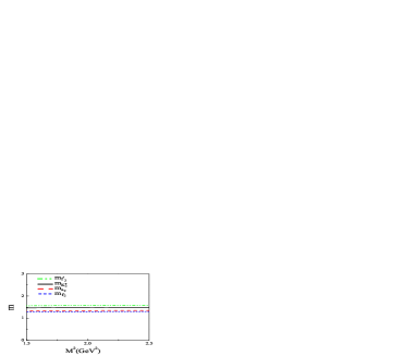
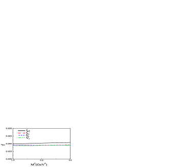
Figure 2: The dependence of the tensor meson masses on the Borel parameter $M^{2}$ (left). The same as it but for the decay constants (right).

The results of our analysis for the masses of the tensor mesons for different values of $\Delta$ and $M^{2}=2$, are given in Table 1. This table contains also the experimental quantities of the light tensor mesons. As it is seen, our values for $\Delta_{2}=0.25~{}GeV$ are in very good agreement with the experimental values.

Table 1: Comparison of the light tensor meson masses in this work for various $\Delta$, where $\Delta_{1}=0.20~{}GeV,\Delta_{2}=0.25~{}GeV,\Delta_{3}=0.30~{}GeV$, with the experimental values in $GeV$.

Mass	$m_{T}(\Delta_{1})$	$m_{T}(\Delta_{2})$	$m_{T}(\Delta_{3})$	EXP PDG
$m_{K_{2}^{*}}$	$1.39\pm 0.22$	$1.42\pm 0.31$	$1.46\pm 0.42$	$1.43$
$m_{a_{2}}$	$1.28\pm 0.21$	$1.31\pm 0.30$	$1.35\pm 0.41$	$1.32$
$m_{f_{2}}$	$1.25\pm 0.21$	$1.28\pm 0.30$	$1.35\pm 0.41$	$1.28$
$m_{f^{\prime}_{2}}$	$1.49\pm 0.23$	$1.52\pm 0.33$	$1.55\pm 0.45$	$1.53$

In Table 2, our results for the decay constants of the tensor mesons for different values of $\Delta$ and $M^{2}=2$, as well as the obtained results via other ways in the framework of the SR are presented. It should be noted that the decay constant $f_{T}$ defined in Cheng ; Bagan differs from ours by a factor of $1/(2m_{T})$. Therefore, their values have been rescaled and then presented in Table 2.

Table 2: Comparison of the decay constant values of the tensor mesons in this work for various $\Delta$, where $\Delta_{1}=0.20~{}GeV,\Delta_{2}=0.25~{}GeV,\Delta_{3}=0.30~{}GeV$, with the values obtained by others (in units of $10^{-3}$).

Decay Constant	$f_{T}(\Delta_{1})$	$f_{T}(\Delta_{2})$	$f_{T}(\Delta_{3})$	Cheng	Aliev	Shifman	Bagan
$f_{K_{2}^{*}}$	$34\pm 3$	$36\pm 4$	$39\pm 5$	$41$	$50$	—	—
$f_{a_{2}}$	$34\pm 3$	$37\pm 4$	$40\pm 5$	$41$	—	—	—
$f_{f_{2}}$	$35\pm 3$	$38\pm 4$	$41\pm 6$	$40$	—	$40$	$52-72$
$f_{f^{\prime}_{2}}$	$33\pm 2$	$35\pm 3$	$37\pm 4$	$42$	—	—	$37-50$

The results derived by us, especially for $\Delta_{3}=0.30~{}GeV$, are in consistent agreement with other values.

The errors are estimated by the variation of the Borel parameter $M^{2}$, the variation of the continuum threshold $s_{T}$, and uncertainties in the values of the other input parameters. The main uncertainty comes from the continuum thresholds of the central value, while the other uncertainties are small, constituting a few percent.

References

(1)
W. Wang, Phys. Rev. D 83, 014008 (2011).
(2)
S. V. Dombrowski, Nucl. Phys. Proc. Suppl. 56, 125 (1997).
(3)
C. Amsler et al., Particle Data Group, Phys. Lett. B 667, 1 (2008).
(4)
D. M. Li, H. Yu, and Q. X. Shen, J. Phys. G 27, 807 (2001).
(5)
H. Y. Cheng, Y. Koike, and K. C. Yang, Phys. Rev. D 82, 054019 (2010).
(6)
M. A. Shifman, A. I. Vainshtein, and V. I. Zakharov, Nucl. Phys. B 147,
385 (1979).
(7)
P. Colangelo, and A. Khodjamirian, in At the Frontier of Particle
Physics/Handbook of QCD, edited by M. Shifman (World Scientific,
Singapore, 2001), Vol. III, p. 1495.
(8)
T. M. Aliev, and M. A. Shifman, Phys. Lett. B 112, 401 (1982); Sov. J.
Nucl. Phys. 36 (1982) 891 [Yad. Fiz. 36 (1982) 1532].
(9)
T. M. Aliev, K. Azizi, and V. Bashiry, J. Phys. G 37, 025001 (2010).
(10)
E. Bagan and S. Narison, Phys. Lett. B 214, 451 (1988).
(11)
H. Terazawa, Phys. Lett. B 246, 503 (1990).
(12)
M. Suzuki, Phys. Rev. D 47, 1043 (1993).
(13)
F. X. Lee, S. Moerschbacher, and W. Wilcox, Phys. Rev. D 78, 094502
(2008).
(14)
E. Katz, A. Lewandowski, and M. D. Schwartz, Phys. Rev. D 74, 086004
(2006).
(15)
P. Colangelo, and A. Khodjamirian, arXiv: hep-ph/0010175; A. V.
Radyushkin, arXiv: hep-ph/0101227.
(16)
V. M. Belyaev, and B. L. Ioffe, JETP 56, 493 (1982).
(17)
M. Q. Huang, Phys. Rev. D 69, 114015 (2004).
(18)
B. L. Ioffe, Prog. Part. Nucl. Phys. 56, 232 (2006).
(19)
J. Beringer et al., Particle Data Group, Phys. Rev. D 86, 010001
(2012).