Formation Mechanism of Bound States in Graphene Point Contacts

Abstract

Electronic localization in narrow graphene constrictions are theoretically studied, and it is found that long-lived ($\sim 1~{}\mbox{ns}$) quasi-bound states (QBSs) can exist in a class of ultra-short graphene quantum point contacts (QPCs). These QBSs are shown to originate from the dispersionless edge states that are characteristic of the electronic structure of generically terminated graphene in which pseudo time-reversal symmetry is broken. The QBSs can be regarded as interface states confined between two graphene samples and their properties can be modified by changing the sizes of the QPC and the interface geometry. In the presence of bearded sites, these QBS can be converted into bound states. Experimental consequences and potential applications are discussed.

I Introduction

Quantum point contacts (QPCs), which are narrow constrictions connecting two wider samples, constitute fundamental building blocks of miniaturized devices such as quantum dots and qubits Houten1996 ; Zhang2011 . Being open systems, QPCs are usually incapable of supporting atomistically small quasi-bound states (QBSs) Houten1992 ; Thomas2010 . However, if they exist, QBSs can radically affect the properties of a system. For example, they might trap electrons and produce local magnetic moments Iqbal2013 ; Bauer2013 ; Yakimenko2013 ; Yoon2009 ; Rejec2006 ; Hirose2003 ; Thomas1996 ; Thomas1998 , which can cause spin-dependent transpsort through a QPC.

Graphene, which is a one-atom-thick carbon sheet, has attracted tremendous attention in the past decade owing to its novel physical properties and potential applications for future electronic devices Geim2007 ; White2007a . Nanostructures made of graphene can be patterned using lithography technique Tapaszto2008 . Graphene QPCs have been fabricated and extensively studied Girdhar2013 ; Guttinger2012 ; Ozyilmaz2007 ; Terres2011 ; Han2010 ; Stampfer2008 ; Darancet2009 ; Todd2008 . A shortest-possible QPC, which is made of a single hexagon and makes an aperture for electrons, has been theoretically examined Darancet2009 , and typical wave diffraction patterns were predicted. To date, all graphene QPCs investigated have been designed to connect the middle of samples, as sketched in FIG. 1(a), and no signatures of electron localization were found in the ballistic limit.

In this paper, we systematically study a different type of graphene QPC, where two graphene samples are connected near the edges as shown in FIG. 1(b). In these QPCs, the edge states, which appear on zigzag-shaped graphene edges at zero energy Fujita1996a ; Fujita1996b ; Enoki2013 , are shown to dominate the electronic transport properties. For half graphene plane with a perfect zigzag edge, the edge states are non-bonding and are located on only one of the two sublattices. It has been shown that the edge states are crucial in determining the magnetic and transport properties of nanostructured graphene systems Rycerz2007 ; Wakabayashi2007 ; White2010 ; White2008 ; White2007 ; Wakabayashi2002 ; Fujita1996b ; Wakabayashi2012 ; Karimi2012 ; Akhmerov2008 ; Deng2013 .

In conventional graphene QPCs, the edge states have negligible effects because they are far from the QPC. However, we show that electrons can be localized in QPCs as depicted in FIG. 1(b), i.e., where edge states located on different sublattices are coupled, resulting in the formation of QBSs. These QBSs can live up to $\tau_{QBS}\sim\mbox{ns}$ for sufficiently large samples and their wave functions spread over only a few lattice constants. Their lifetimes can be tuned by changing the geometry of the QPC and the size of the sample, whereas their energies $\varepsilon_{QBS}$ are found to be insensitive to sample dimensions. These QBS may be used as few-level quantum dots and artificial atoms.

We organize the paper as follows. In Section II, we classify the edge-connected graphene QPCs into three classes and give a brief overview of the results. In Section III, we describe the formation mechanism of QBSs using the Green’s function approach. In Section IV, we apply the theory to an example QPC, where analytical results are obtained and compared to numerical calculations. Finally, in Section V, we discuss some experimental signatures and potential applications.

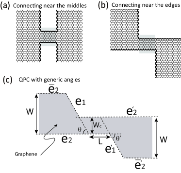
Figure 1: (a) Schematic of the QPC connecting samples near the middle. (b) Schematic of the QPC connecting samples near the edge, where edge states can play an important role in electron transmission. (c) Schematic of the generic graphene QPCs connecting samples near the edge. Both samples infinitely extend along the edges $e_{2}$ and $e^{\prime}_{2}$. The angles $\theta$ and $\theta^{\prime}$ can be taken to be the same without loss of generality.

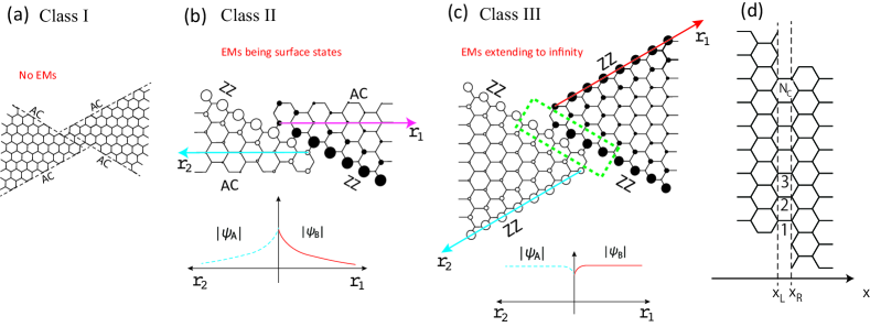
Figure 2: Classification of QPCs connecting samples near the edges. (a) Example of Class I, which has all AC edges and no edge state. QPCs in this class are similar to QPCs connecting near the middle of samples. (b) Example of Class II, for which has the interface edges are ZZ but the extending edges are AC. In this class the edge states exponentially decay from the interface and are localized near the interfaces, i.e. bound states. Here the white (black) circles indicate the charge density of edge states on the A (B) sublattice sites. The schematic charge densities of edge state are for isolated samples Shimomura2011 . (c) Example of Class III, for which the extending edges are ZZ whereas the interfacing edges can be either ZZ (as in the example shown here) or AC (as in the example shown in FIG. 3). In this class, edge states also exist. However, they are not bound states as indicated by the schematic wave functions of semi-infinite isolated samples (bottom panel). Nevertheless, bound states emerge when QPCs are present. (d) Enlarged view of QPC [indicated by the dashed rectangle in panel (c)]. The QPC contains $N_{c}$ connecting bonds.

II Overview

Figure 1(c) schematically shows the QPC that connects two graphene samples of the same width $W$ near their edges. This QPC can be taken as an aperture for electron waves. The length and width of the QPC are $L$ and $W_{c}$, respectively. Each graphene sample is geometrically confined by three edges, which are denoted by $e_{1}$, $e_{2}$, and $\bar{e}_{2}$ ($e^{\prime}_{1}$, $e^{\prime}_{2}$, and $\bar{e^{\prime}}_{2}$) for the left-hand (right-hand) sample. We have assumed that $e_{2}$ ($e^{\prime}_{2}$) is parallel with $\bar{e}_{2}$ ($\bar{e^{\prime}}_{2}$). This condition is not necessary but facilitates the analysis. The interface edges (i.e., $e_{1}$ and $e^{\prime}_{1}$) are assumed to be parallel for a smooth joint. Furthermore, we presume each edge to be either a perfect armchair (AC) or zigzag (ZZ) (i.e., the angles $\theta$ and $\theta^{\prime}$ are integers of $\frac{\pi}{6}$). According to the edge structure, we can classify the QPCs into three classes of configurations as shown in FIG. 2. The details of each class are described below.

(Class I) All edges in a QPC are AC, as shown in FIG. 2(a). Because there are no edge states in this class, the resulting QPCs resemble conventional QPCs and are therefore not further addressed in this paper.

(Class II) The edges $e_{1}$ and $e^{\prime}_{1}$ are ZZ, whereas the edges $e_{2}$ and $e^{\prime}_{2}$ are AC. An example is given in FIG. 2(b). In this class edge states appear on $e_{1}$ and $e^{\prime}_{1}$. However, these edge states are no more than surface states, whose wave functions are bound to $e_{1}$ ($e^{\prime}_{1}$), i.e., the wave function exponentially decays away from the QPC as schematically shown in FIG. 2(b). Because the edge states do not extend along $e_{2}$ ($e^{\prime}_{2}$), they do not directly participate in electronic transport. Therefore, this class of QPCs simply admixes the surface states bound on $e_{1}$ with those on $e^{\prime}_{1}$, yielding (quasi-) bound states.

(Class III) Our main interest lies in this third class. The interface edges $e_{1}$ and $e^{\prime}_{1}$ can be either AC or ZZ, while the edges $e_{2}$ and $e^{\prime}_{2}$ (and hence $\bar{e}_{2}$ and $\bar{e^{\prime}}_{2}$) are ZZ. There are two bunches of edge states located on different sublattices; these edge states extend along $e_{2}$ ($e^{\prime}_{2}$) and $\bar{e}_{2}$ ($\bar{e^{\prime}}_{2}$). In FIG. 2(c), we show an example of all ZZ edges. A different geometry is shown in FIG. 3, where the interface edges are AC.

The QBSs are formed because of the non-bonding nature of the edge states of the left and right samples (i.e. edges $e_{2}$ and $e_{2}^{\prime}$). The QBS energy $\pm\varepsilon_{QBS}$ and lifetime $\tau_{QBS}$ are sensitive to the ratio $W_{c}/W$. QBSs have a long lifetime only for $W_{c}\ll\frac{W}{2}$. The quantity $\tau_{QBS}$ rapidly increases with $W$ according to a power law; $\tau_{QBS}\sim\left(\frac{W}{W_{0}}\right)^{3}$ps, whereas $\varepsilon_{QBS}$ is insensitive to $W$. Here $W_{0}$ is a length scale, which is around $86a\approx 21\mbox{nm}$ for $\theta=\theta^{\prime}=\frac{\pi}{2}$. In general, QBS causes resonant scattering which leads to a resonance peak in the conductance $g$ of the QPC. For large $W$, $g$ takes on a symmetric Breit-Wigner form,

$$g\approx g_{m}\frac{\Gamma^{2}_{QBS}}{(\varepsilon_{F}-\varepsilon_{QBS})^{2}+\Gamma^{2}_{QBS}},$$ (1)

where $g_{m}\sim 1$ in units of $g_{0}=\frac{2e^{2}}{h}$, $\varepsilon_{F}$ is the Fermi level and $\Gamma_{QBS}=\frac{\hbar}{\tau_{QBS}}$ denotes the level-broadening parameter. For finite $W$, the background contribution leads to an asymmetric lineshape for $g$, i.e., Fano resonances.

III Theory: $T$-Matrix Formalism

III.1 Model

In this section, we analyze the electronic properties of graphene QPCs using transition matrix ($T$-matrix) formalism based on the nearest-neighbor tight-binding model Economou1979 . We refer to the geometry shown in FIG. 2(c) for clarity. The enlarged view of the QPC is displayed in FIG. 2(d), where the two graphene samples are connected via $N_{c}$ connecting bonds. Each bond has a left- and right-hand end lying on $x=x_{L}$ and $x=x_{R}$, respectively. The end sites on $x=x_{L}$ ($x_{R}$) are labeled $i_{L}$ ($i_{R}$), where the index $i_{L}$ ($i_{R}$) runs over $1,2,\cdots,N_{c}$. The graphene edge along $x=x_{L}$ ($x_{R}$) corresponds to edge e₁ (e${}_{1}^{\prime}$) in FIG. 1(c).

The total Hamiltonian of the system can be written as $H=H_{L}+H_{R}+V$, where $H_{L}$ ($H_{R}$) describes the left (right) isolated graphene sample while $V$ stands for the QPC. Explicitly, we have

$$V=\sum^{N_{c}}_{i_{L}=1}\sum^{N_{c}}_{i_{R}=1}\gamma_{i_{L},i_{R}}\left(|i_{L}\rangle\langle i_{R}|+{\rm h.c.}\right),$$ (2)

where $\gamma_{i_{L},i_{R}}=-\gamma_{0}\delta_{i_{L},i_{R}}$ with $\gamma_{0}\approx 2.7\mbox{eV}$ and $\delta_{i,j}$ is the Kronecker’s function. We introduce the bare Green’s function, $G_{0}(\varepsilon)=(\varepsilon+i0_{+}-H_{0})^{-1}$, with $H_{0}=H_{L}+H_{R}$. For later use, we resolve the diagonal elements of $G_{0}$ as follows:

$$G^{i,i}_{0}(\varepsilon)=\sum_{\mu}|\psi_{i;\mu}|^{2}(\varepsilon+i0_{+}-\varepsilon_{\mu})^{-1},\quad\psi_{i;\mu}=\langle i|\mu\rangle,$$ (3)

where $|\mu\rangle$ are the eigenstates of $H_{0}$, i.e., $H_{0}|\mu\rangle=\varepsilon_{\mu}|\mu\rangle$. Now the $T$-matrix can be defined as

$$T(\varepsilon)=(1-VG_{0})^{-1}V=V+VG_{0}V+(VG_{0})^{2}V+\cdots$$ (4)

where $0_{+}$ denots an infinitesimal positive number. In principle, this matrix captures all physical effects arising from scattering at the QPC. The QBS can be found by searching for the poles of $T(\varepsilon)$.

For further analysis, let us closely inspect the bonding character at the interface. We note that the $N_{c}$ connecting bonds fall into two categories: strongly connecting bonds (SCBs) and weakly connecting bonds (WCBs). Introducing the bare local density of states (LDOS) on atomic site $i$ at energy $\varepsilon$ as $\rho_{0}(\varepsilon,i)=-\frac{1}{\pi}Im[G^{i,i}_{0}(\varepsilon)]$, a SCB is then defined to have nonvanishing $\rho_{0}(0,i)$ on both $i=i_{L}$ and $i=i_{R}$ where $i_{L}$ and $i_{R}=i_{L}$ denote the sites belonging to this bond. Similarly, a WCB is defined to lack this property. In the QPC shown in FIG. 2(c), all connecting bonds are SCBs. However, in the QPC shown in FIG. 3, which also belongs to Class III, the SCBs and WCBs alternate with each other.

III.2 Energy and Lifetime of QBS

In general, it is a formidable task to evaluate $T$ exactly. Here we use two approximations. First, we neglect all inter-bond transitions (i.e., $T_{i_{R},i_{L}}\propto\delta_{i_{R},i_{L}}$). This is reasonable, because these transitions are higher-order processes in $G_{0}$ compared with intra-bond transitions. Second, we assume $G^{i,i}_{0}\approx 0$ at low energies if $i$ belongs to a WCB, which can be justified in the limit $\frac{W}{2}\gg W_{c}$. Then, we can easily derive that $T_{i_{R},i_{L}}(\varepsilon)\approx-\gamma_{0}\delta_{i_{R},i_{L}}$ for WCBs and that

$$T_{i_{R},i_{L}}(\varepsilon)\approx\frac{-\gamma_{0}\delta_{i_{R},i_{L}}}{1-\gamma^{2}_{0}G^{i_{L},i_{L}}_{0}(\varepsilon)G^{i_{R},i_{R}}_{0}(\varepsilon)},$$ (5)

for SCBs note0 . Basically, this expression describes the physical processes in which an electron travels back and forth between the sites $i_{L}$ and $i_{R}$, in analogy with back-and-forth bounces experienced by an electron sandwiched between two potential barriers Thomas2010 . Note that such processes increase returning probability and are responsible for the formation of QBSs.

The energy and broadening of QBS can be determined by seeking the poles of Eq. (5). Rewriting $\gamma^{2}_{0}G^{i_{L},i_{L}}_{0}(\varepsilon)G^{i_{R},i_{R}}_{0}(\varepsilon)=R^{i_{L},i_{R}}(\varepsilon)+i\cdot I^{i_{L},i_{R}}(\varepsilon)$, the poles $z_{QBS}=\varepsilon_{QBS}+i\Gamma_{QBS}$ can be obtained via

$$1-R^{i_{L},i_{R}}(z_{QBS})-i\cdot I^{i_{L},i_{R}}(z_{QBS})\approx 0.$$ (6)

As will be shown later, in the large $W$ limit, we have

$$G^{i_{\tau},i_{\tau}}_{0}\approx\frac{1}{\varepsilon}\cdot B_{\tau}-\frac{i}{\gamma_{0}}\cdot C_{\tau},$$ (7)

where $\tau=$L or R. $B_{\tau}$ and $C_{\tau}$ are real values, which vary from bond to bond. Later, we will see that $C_{\tau}$ decreases to zero with increasing $W$ following a power law whereas $B_{\tau}$ approaches a constant $B_{\tau,\infty}$. Upon substitution, we immediately find

$$\begin{pmatrix}\varepsilon_{QBS}\\ \Gamma_{QBS}\end{pmatrix} \approx \frac{-\gamma_{0}}{2(1+C_{L}C_{R})}$$ (8)

$$\cdot \begin{pmatrix}\pm\sqrt{4B_{L}B_{R}-(B_{L}C_{R}-B_{R}C_{L})^{2}}\\ B_{L}C_{R}+C_{L}B_{R}\end{pmatrix}$$

From this it follows that, (1) there is a pair of QBS with each SCB, whose energies are symmetric about zero; (2) the energy of the QBS is not sensitive to the sample width, i.e., $\varepsilon_{QBS}\approx\pm\gamma_{0}\sqrt{B_{L}B_{R}}\approx\pm\varepsilon_{\infty}=\pm\gamma_{0}\sqrt{B_{L,\infty}B_{R,\infty}}$; (3) the QBS has a broadening, $\Gamma_{QBS}$, which shrinks rapidly with $W$, as explained below.

It proves useful to rewrite Eq. (5) as

$$T_{i_{L}=l,i_{R}=l}(\varepsilon)=-\frac{\gamma_{0}\varepsilon^{2}}{(\varepsilon-z_{QBS,l})(\varepsilon+z^{*}_{QBS,l})},$$ (9)

where we have used Eq. (7) and $l$ indicates the $l$-th SCB. The maximum of $|T_{i_{L}=l,i_{R}=l}(\varepsilon)|$ occurs when $\varepsilon=\varepsilon_{QBS,l}$, for which we have

$$T_{i_{L}=l,i_{R}=l}(\varepsilon_{QBS,l})=-i\gamma_{0}\frac{\varepsilon_{QBS,l}}{2\Gamma_{QBS,l}}\gg T_{i_{L}\neq l,i_{R}\neq l}(\varepsilon_{QBS,l}).$$ (10)

Evidently, the $l$-th SCB predominates for $\varepsilon\sim\varepsilon_{QBS,l}$.

Now we establish Eq. (7). For this purpose, we decompose Eq. (3) into its real and imaginary parts:

$$G^{i_{\tau},i_{\tau}}_{0}(\varepsilon)=\sum^{\prime}_{\mu}|\psi_{i_{\tau};\mu}|^{2}(\varepsilon-\varepsilon_{\mu})^{-1}-i\pi\rho_{0}(\varepsilon,i_{\tau})$$ (11)

where $i_{\tau}$ belongs to a SCB, $\rho_{0}(\varepsilon,i_{\tau})=\sum_{\mu}|\psi_{i_{\tau};\mu}|^{2}\delta(\varepsilon-\varepsilon_{\mu})$ is the aforementioned LDOS on site $i_{\tau}$ and $\delta$ denotes the Dirac $\delta$ function while the prime indicates the principal value of the sum (which can be turned into an integral). The $\mu$ denotes either an extended state or an edge state. In the sum, the contributions from the extended states are of the order $W^{-3}$note2 and can then be neglected for large $W$, whereas the contributions from the edge states are roughly independent of $W$. Therefore, considering that edge states have zero energies at large $W$, we arrive at the $G^{i,i}_{0}$ as given in Eq. (7), with the coefficients given by

$$B_{\tau} = \sum_{\mu=\mbox{edge states}}|\psi_{i_{\tau};\mu}|^{2},$$

$$C_{\tau} = -\pi\gamma_{0}\rho_{0}(\varepsilon_{QBS},i_{\tau}).$$ (12)

From $B_{\tau}$ one determines $\varepsilon_{QBS}$. The quantity $C_{\tau}$ is found by comparing Eqs. (7) and $(\ref{Go})$. Equations (5), (7) and (12) constitute the foundation of the present theory. They are applicable to all QPC configurations exemplified in FIG. 2 in the limit $\frac{W}{2}\gg W_{c}$. In the next section, we discuss prototypical examples.

In the limit $W\rightarrow\infty$, the edge states approach those of two isolated half infinite graphene planes. Accordingly, the quantity $B_{\tau}$ tends to a constant $B_{\tau,\infty}$ given by Eq. (12) with the edge states of two half planes. Simultaneously, $C_{\tau}$ tends to zero, since $\rho_{0}(\varepsilon_{QBS},i_{\tau})$ comes from only extended states whose wave functions vanish on $i_{\tau}$ as $W/W_{c}\rightarrow\infty$.

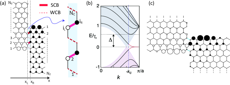
Figure 3: (a) Class-III QPC with rectangular corners with $N_{c}=5$ connecting bonds. In this QPC, the edge states have amplitude on sublattice A (indicated by white circle) for the left-hand graphene sample, whereas they have amplitude on sublattice B (indicated black circle) for the right-hand graphene sample. The SCBs and WCBs alternate with each other. (b) Energy spectrum for a semi-infinite ribbon consisting of $N_{z}=6$ zigzag chains. Shaded areas indicate the spectrum of bulk graphene. Edge states appear in $k_{c}<k\leq\pi/a$ (red segments). The black lines indicate the extended states. (c) Magnitude of the QBS wave function $\langle j|QBS\rangle$ in the vicinity of a SCB assuming a symmetric boundary condition, which can be observed in STM. The calculation was done for $N_{z}=50$ and $\varepsilon_{QBS}\approx 0.04$.

III.3 Wave Functions of QBS

To derive the QBS wave function, we shall consider the QBS associated with the $l$-th SCB, for which $i_{L}=i_{R}=l$. In the conventional scattering theory Economou1979 , the state vector is given by $|QBS,l\rangle=|\psi_{0}\rangle+G_{0}T|\psi_{0}\rangle$, where $H_{0}|\psi_{0}\rangle=\varepsilon_{QBS,l}|\psi_{0}\rangle$. We have explicitly included the index $l$ to indicate the QBS in question. To specify the QBS wave function, $\Psi_{l}(j)\equiv\langle j|QBS,l\rangle$, where $j$ denotes an arbitrary site in the entire system, we have to impose boundary conditions on $\langle j|\psi_{0}\rangle$. Two types of boundary conditions are considered here.

(Type I) This type assumes an open system and is appropriate for studying transport properties. The $\Psi_{l}(j)$ is supposed to describe an electron wave incident from the left-hand sample, tunneling through the QPC and partailly transmitted to the right-hand sample. The $\langle j|\psi_{0}\rangle$ describes the superposition of the incident wave and the totally reflected wave. We then find

$$\Psi_{l}(j) \approx \langle j|\psi_{0}\rangle$$ (13)

$$+ T_{i_{L},i_{L}}(\varepsilon_{QBS,l})G^{j,i_{L}}_{0}(\varepsilon_{QBS,l})\langle i_{L}|\psi_{0}\rangle$$

$$+ T_{i_{R},i_{L}}(\varepsilon_{QBS,l})G^{j,i_{R}}_{0}(\varepsilon_{QBS,l})\langle i_{L}|\psi_{0}\rangle,$$

where $i_{L}=i_{R}=l$. The third term describes the transmitted wave. Note that we have kept only the $l$-th bond, which is reasonable according to Eq. (10).

(Type II) This type assumes a closed system, in which no current flows from left to right. It is suitable for describing scanning tunneling microscopy (STM). We then find

$$\Psi_{l}(j) \approx \langle j|\psi_{0}\rangle+T_{i_{L},i_{R}}(\varepsilon_{QBS,l})$$ (14)

$$\times [G^{j,i_{L}}_{0}(\varepsilon_{QBS,l})\cdot\langle i_{R}|\psi_{0}\rangle$$

$$+ G^{j,i_{R}}_{0}(\varepsilon_{QBS,l})\cdot\langle i_{L}|\psi_{0}\rangle].$$

where $i_{L}=i_{R}=l$. We have neglected the terms headed by $T_{i_{L},i_{L}}$ and $T_{i_{R},i_{R}}$, which are smaller than the retained terms note0 . An example of $\Psi_{l}(j)$ is mapped in FIG. 3(c), where we see that $\Psi_{l}(j)$ extends over only a few lattice constants in space.

IV Example: $\theta=\theta^{\prime}=\frac{\pi}{2}$

Let us illustrate the above theory for the rectangular-corner configuration shown in FIG. 3. In this case, isolated graphene samples are semi-infinite ribbons. Their wave functions can be obtained from those for infinite ribbons, for which analytical solutions have been established Wakabayashi2012 . Thus, the coefficients $B_{\tau}$ and $C_{\tau}$ can be analytically obtained. For convenience, we express the width $W$ in terms of the number of total zigzag chains $N_{z}$ as $W=\frac{a}{2\sqrt{3}}(3N_{z}-2)$.

IV.1 Calculation of $\varepsilon_{QBS}$ and $\Gamma_{QBS}$

The goal is to find the coefficients $B_{\tau}$ and $C_{\tau}$. For this purpose, we need $\psi_{i;\mu}$, the wave function of mode $|\mu\rangle$, which can be represented as a superposition of two counter-propagating waves related by time reversal symmetry appropriate to an ideal zigzag graphene ribbon. They can be easily constructed so we simply quote the results here:

$$\begin{pmatrix}\psi_{i_{L};\mu}\\ \psi_{i_{R};\mu}\end{pmatrix}=\sqrt{\frac{2a}{L}}e^{ika}\sin\left(\frac{ka}{2}\right)\begin{pmatrix}-\Phi_{\mu}(i_{L})\\ \Phi_{\mu}(i_{R})\end{pmatrix}$$ (15)

In Eq. (15), $k\in[0,\pi/a]$ and $L$ denotes the circumference of a virtual zigzag graphene tube used to discretize the values of $k$. $\Phi$ is the transverse component of the wave fuction. Note that $\mu$ is shorthand for a composite index, $(k,u,s)$, where $u=1,\cdots,N_{z}$ counts the subbands and $s=\pm$ is the particle-hole label, as sketched in FIG. 3(b).

Specific to each subband, there is a quantum number $p_{u}$, which is real at any $k$ for $u<N_{z}$ Wakabayashi2012 . However, for $u=N_{z}$, $p$ is real only if $k\in[0,k_{c}]$ and it can be written as $p=\pi+i\eta$ if $k\in(k_{c},\frac{\pi}{a}]$. For this particular subband, in the large $N_{z}$ limit, whereby $k_{c}=\frac{2\pi}{3a}$, it holds as a good approximation that $\varepsilon_{s}(k)\approx 0$ and note4

$$\begin{pmatrix}\Phi_{k,s}(i_{L})\\ \Phi_{k,s}(i_{R})\end{pmatrix}\approx\sqrt{\frac{1-g^{2}_{k}}{2}}\begin{pmatrix}g^{i_{L}-1}_{k}\\ g^{N_{c}-i_{R}}_{k}\end{pmatrix}$$ (16)

for $k>\frac{2\pi}{3a}$. Here $g_{k}=2\cos(ka/2)$. For $k<\frac{2\pi}{3a}$, in the same limit, we instead have $\varepsilon_{s}(k)\approx s(g_{k}-1)$ and

$$\begin{pmatrix}\Phi_{k,s}(i_{L})\\ \Phi_{k,s}(i_{R})\end{pmatrix}\approx\sqrt{\frac{1}{N_{z}}}\begin{pmatrix}\sin(pi_{L})\\ \sin[p(N_{c}+1-i_{R})\end{pmatrix}$$ (17)

where $p\approx(1-\frac{1}{N_{z}})\pi$ and we have dropped the subscript $u$ for this subband. Note that, as shown in Fig. 3(b), this subband is the only one available within the energy window $[-\Delta,\Delta]$, where $\Delta\approx 4\gamma_{0}\cos(\frac{N_{z}-1}{2N_{z}-1}\pi)$.

To evaluate $C_{\tau}$, we may presume that the QBS lies inside the single-channel energy window (i.e., $\varepsilon_{QBS}\in[-\Delta,\Delta]$). Then, the only contribution to $\rho_{0}$, i.e. $C_{\tau}$, comes from the $u=N_{z}$ subband with $k\in[0,\frac{2\pi}{3a}]$, because these are the only states available in that energy window. This assumption, whose validity can be examined by consistency check, implies that the QBS life time is essentially set by the dispersing segment of the lowest subband. By using Eqs. (15) and (17), we obtain

$$\begin{pmatrix}C_{L}\\ C_{R}\end{pmatrix}\approx A\cdot\frac{\pi^{2}}{N^{3}_{z}}\begin{pmatrix}i^{2}_{L}\\ (N_{c}+1-i_{R})^{2}\end{pmatrix}$$ (18)

with $A=-\frac{2a}{L}\cdot\pi\cdot\sum_{0\leq k<\frac{2\pi}{3a}}\sin^{2}\left(\frac{ka}{2}\right)\delta[\varepsilon^{2}_{QBS}-(g_{k}-1)^{2}]$. Transforming it into an integral, we find $A=-\frac{\sin(x_{0})}{2|\varepsilon_{QBS}|}$, with $x_{0}\in(0,\frac{\pi}{3})$ given by $|\varepsilon_{QBS}|=2\cos(x_{R})-1$. The quadratic dependences on $i_{L}$ and $N_{c}$ are notable in Eq. (18), which explains why long-lived QBSs only form when $N_{c}$ is small.

We proceed to estimate $B_{\tau}$. At energies near zero the primary contributions stem from the edge states. Actually, since $p_{u}\approx\frac{u-1}{N_{z}}\pi$ for any extended state [Fig. 3(b)] of any subband in the large $N_{z}$ limit, the total contributions from the low energy sector, i.e., including those with $u\sim N_{z}$, are of the order $\sim N^{-1}_{z}\sum_{u\sim N_{z}}|\sin(\frac{u-1}{N_{z}}\pi)|^{2}\approx N^{-3}_{z}$note2 . Nonetheless, the contribution from the edge states is of order unity, as indicated in Eq. (16). Thus, when $N_{z}$ is large, the edge states dominate. If we neglect the dispersion of these states, which is reasonable for large $N_{z}$, we immediately confirm Eq. (12). Using Eqs. (15) and (16), we find

$$\lim_{N_{z}\rightarrow\infty}\begin{pmatrix}B_{L}\\ B_{R}\end{pmatrix}=\begin{pmatrix}B_{L,\infty}\\ B_{R,\infty}\end{pmatrix}$$

$$= \frac{2a}{L}\sum_{\frac{2\pi}{3a}<k<\frac{\pi}{a}}\sin^{2}(ka/2)(1-g^{2}_{k})\begin{pmatrix}g^{2(i_{L}-1)}_{k}\\ g^{2(N_{c}-i_{R})}_{k}\end{pmatrix}$$

which quickly diminish as $N_{c}$ or $i_{L}$ increases.

Note that the maximum values of $B_{L,\infty}$ and $B_{R,\infty}$ occur at $(N_{c}=2,i_{L}=i_{R}=2)$, in which case one finds $B_{L,\infty}\approx 0.04$ and $B_{R,\infty}\approx 0.21$, leading to $\varepsilon_{\infty}\approx 0.09\gamma_{0}$. Therefore, for most ribbons of interest, we indeed have $\varepsilon_{\infty}\in[-\Delta,\Delta]$, which is consistent with our initial assumption note3 . Another case of special interest is $N_{c}=3$, for which we find $B_{L,\infty}=B_{R,\infty}\approx 0.04$, yielding $\varepsilon_{\infty}\approx 0.04\gamma_{0}$. We then see that the $\varepsilon_{\infty}$ depends strongly on $N_{c}$. The parameters for other interesting cases have also been calculated and are tabulated in Table I.

Table 1: Theoretically evaluated parameters for certain SCBs $(N_{c},i_{L})$ (obviously $i_{R}=i_{L}$ for a given bond) in the configuration shown in FIG. 3. From Eqs. (8) and (19), we see that $\Gamma_{QBS}N^{3}_{z}$ (given in the last column) is independent of $N_{z}$. All energies are in units of $\gamma_{0}$.

$(N_{c},i_{L})$	$B_{L,\infty}$	$B_{R,\infty}$	$\varepsilon_{\infty}$	$|A|$	$C_{L}\cdot N^{3}_{z}$	$C_{R}\cdot N^{3}_{z}$	$\Gamma_{QBS}\cdot N^{3}_{z}$
(2,2)	0.04	0.21	0.09	9.7	386.7	96.7	42.5
(3,2)	0.04	0.04	0.04	21.8	870	870	34.8
(4,2)	0.04	0.017	0.026	33.5	1338	3011	71.5
(4,4)	0.009	0.21	0.044	19.7	3149	196.8	331.6

IV.2 Spatial Profile of QBS

To visualize the QBS in real space, we calculated the wave function of the QBS according to Eq. (14) for symmetric boundary condition. We neglected the first term in these equations, so the spatial profile of the QBS is completely determined by $G^{j,i_{L}}_{0}$ and $G^{j,i_{R}}_{0}$, which can be easily evaluated numerically using the resolution of Eq. (3). In FIG. 3(c), we show the results for the symmetric configuration $(N_{c}=3,i_{L}=2)$. As expected, the amplitudes are concentrated about the SCB, spreading over a few lattice constant. This distribution can be observed in STM (see Section V). It is worth noting that the SCB resembles a molecular junction between the graphene samples.

IV.3 Conductance

Ultra-narrow QPCs usually strongly reflect incident electron waves, as would be anticipated from diffraction theory in the sub-wavelength regimeBethe1944 . However, such reflections can be suppressed due to resonant tunneling from QBSs. In what follows, we calculate the conductance $g$ of the QPC shown in FIG.3(a) and derive Eq. (1).

We focus on the single-channel regime, i.e., $\varepsilon\in(0,\Delta)$, where the modes can each be labeled by just a wave number. We use $k$ and $q$ to denote the wave numbers for the left- and right-hand samples, respectively. Following standard tunneling theoryBardeen1961 , we obtain the conductance at zero temperature as

$$g=L^{2}v^{-2}_{F}|\langle q=k_{F}|T|k=k_{F}\rangle|^{2},$$ (20)

where $v_{F}=\left(\frac{d\varepsilon_{k}}{dk}\right)_{k=k_{F}}\approx-a\gamma_{0}\sin(k_{F}a/2)$ and $k_{F}\in(0,\frac{2\pi}{3a})$ denote the Fermi velocity (in units of $\hbar=1$) and Fermi wave number, respectively. By using Eq. (5), we find

$$\langle q|T|k\rangle\approx-\gamma_{0}\sum_{WCB}\psi^{*}_{i_{R},q}\psi_{i_{L},k}+\sum_{SCB}\psi^{*}_{i_{R},q}\psi_{i_{L},k}T_{i_{R},i_{L}},$$

Substituting this in Eq.(20), we find $g=g_{w}+g_{s}+g_{ws}$, where $g_{w}$ ($g_{s}$) involves only WCBs (SCBs) whereas $g_{ws}$ involves both SCBs and WCBs. Explicitly, we have

$$\begin{pmatrix}g_{w}\\ g_{ws}\\ g_{s}\end{pmatrix}=L^{2}v^{-2}_{F}\cdot\begin{pmatrix}\gamma^{2}_{0}|\sum_{l=WCB}\psi^{*}_{i_{R}=l;k_{F}}\psi_{i_{L}=l;k_{F}}|^{2}\\ -\gamma_{0}\sum_{l=SCB}\sum_{l^{\prime}=WCB}\psi^{*}_{i_{R}=l^{\prime},k_{F}}\psi_{i_{L}=l^{\prime},k_{F}}\psi^{*}_{i_{R}=l,k_{F}}\psi_{i_{L}=l,k_{F}}T_{i_{R}=l,i_{L}=l}(\varepsilon_{F})\\ |\sum_{l=SCB}\psi^{*}_{i_{R}=l;k_{F}}\psi_{i_{L}=l;k_{F}}T_{i_{R}=l,i_{L}=l}(\varepsilon_{F})|^{2}\end{pmatrix}$$ (21)

For $\varepsilon_{F}$ near the energy of a QBS, these terms scale with $N_{z}$ as follows,

$$g_{w}\sim N^{-6}_{z},\quad g_{ws}\sim N^{-3}_{z},\quad g_{s}\sim N^{0}_{z}.$$ (22)

which can be shown on the basis of two observations. Firstly, from Eqs. (15) and (17) it follows that $\psi_{i_{\tau};k}\sim N^{-3/2}_{z}$ in the limit $N_{c}\ll\frac{N_{z}}{2}$. Secondly, from Eqs. (9) and (10) it follows that $T_{i_{R}=l,i_{L}=l}\sim-\gamma_{0}N^{3}_{z}$ if $\varepsilon_{l,QBS}\sim\varepsilon_{F}$ or $T_{i_{R}=l,i_{L}=l}\approx-\gamma_{0}$ otherwise. From this, we see that in the large-$N_{z}$ limit the dominant contribution to $g_{ws}$ and $g_{s}$ stems from the SCB whose energy is the closest to $\varepsilon_{F}$. Now the scaling becomes clear: in $g_{w}$, the wave functions contribute the $N^{-6}_{z}$ factor; in $g_{ws}$, this factor is raised by $N^{3}_{z}$ due to the $T$-matrix element, which contributes a $N^{3}_{z}$ factor; in $g_{s}$, two $T$-matrix elements appear and contribute $N^{6}_{z}$, which exactly cancels the $N^{-6}_{z}$ from the wave functions.

The above analysis shows that, for $\varepsilon_{F}$ close to the energy of a QBS, the $g_{w}$ and $g_{ws}$ can be neglected for large $N_{z}$. Thus, we find

$$g\approx g_{s}=L^{2}v^{-2}_{F}|\psi^{*}_{i_{R}=l;k_{F}}\psi_{i_{L}=l;k_{F}}T_{i_{R}=l,i_{L}=l}(\varepsilon_{F})|^{2}$$ (23)

where $\varepsilon_{F}$ is near $\varepsilon_{QBS,l}$. By Eqs. (9) and (17), this expression can be reduced to Eq. (1), with

$$g_{m}=4\sin^{2}(k_{l}a/2)|\Phi^{*}_{k_{F}}(i_{R}=l)\Phi_{k_{F}}(i_{L}=l)|^{2}\left(\frac{\varepsilon_{QBS,l}}{\Gamma_{QBS,l}}\right)^{2}\sim N^{0}_{z}$$ (24)

where $k_{l}\approx\frac{2\pi}{3a}$ is given by $\varepsilon_{k_{l}}=\varepsilon_{QBS,l}\sim 0$. With the parameters given in Table I, it is easy to see that $g_{m}\approx 1$. We emphasize that Eq. (1) gives a good description only when $N_{c}\ll\frac{N_{z}}{2}$. Otherwise, additional contributions from WCBs and overlaps between adjacent QBS make the $g$ asymmetric and more similar to a Fano resonance.

IV.4 Numerical Calculations

To verify the above results, we have performed numerical calculations based on the Landauer formalism and mode-matching method. Details of the scheme will be presented elsewhere.

The calculated conductances for wide ribbons with $N_{c}=2,3,4$ are presented as circles in FIG. 4. For $N_{c}=2,3$, one resonance peak is observed in the entire single-channel regime, as shown in FIG. 4(a). Such peaks are interpreted as consequences of QBS, whose energy and lifetime set the position and half-width of the peaks. As seen in FIG. 4(a), the line-shape of each peak can be well captured by Eq. (1), which is a Lorentzian (solid curves). For $N_{c}=4$, as shown in FIG. 4(b), two peaks are observed. The lower energy peak is very sharp whereas the higher energy peak is much broader. These peaks are identified with QBSs belonging to the two SCBs, $(N_{c}=4,i_{L}=2)$ and $(N_{c}=4,i_{L}=4)$. The line-shape can be described by a superposition of two Lorentzians, as noted in FIG. 4(b).

In FIG. 5 we examine the $N_{z}$ dependences of three quantities: $g_{m}$, $\varepsilon_{QBS}$ and $\Gamma_{QBS}$ in FIGs. 5(a), (b) and (c), respectively. According to the theory, we expect (1) the $g_{m}$ to be roughly independent of $N_{z}$, (2) the $\varepsilon_{QBS}$ to converge to $\varepsilon_{\infty}$ and (3) the $\Gamma_{QBS}$ to decrease as $N^{-3}_{z}$. All these features are borne out in numerical calculations, as evident in FIGs. 5 (a), (b) and (c). We notice a weak dependence of $g_{m}$ and $\varepsilon_{QBS}$ on the parity of $N_{z}$. This odd-even effect gradually disappears when $N_{z}$ increases beyond $\sim 250$, which may be understood by observing that the edge state dispersion can be written as $\varepsilon_{s}(k)\approx 2s(-1)^{N_{z}+1}[1+2\cos(ka)]g^{N_{z}}_{k}$ in the large $N_{z}$ limit. The factor $(-1)^{N_{z}+1}$ may be the origin of such effects. For sufficiently large $N_{z}$ ($N_{z}>\sim 250$), we have $\varepsilon_{s}(k)<\varepsilon_{\infty}$ for all $k\in(\frac{2\pi}{3a},\frac{\pi}{a}]$. Eq. (7) still holds and we have $[B_{L},B_{R}]\approx\frac{2a}{L}\sum_{k,s}\sin^{2}(\frac{ka}{2})(1-g^{2}_{k})(1-\varepsilon_{s}(k)/\varepsilon_{\infty})^{-1}[g^{2(i_{L}-1)}_{k},g^{2(N_{c}-i_{R})}_{k}]$, which does not display any parity effect. However, for $N_{z}$ not that large ($N_{z}<\sim 250$), then $\varepsilon_{\infty}$ will cut $\varepsilon_{s}(k)$ and parity effects can appear. Nonetheless, this case is not amenable to analytical expressions and will not be further discussed.

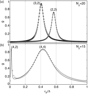
Figure 4: Theory versus numerical calculations: energy dependence of conductance $g$ for the QPC shown in FIG. 3. Circles represent numerical calculations while solid lines indicate fitting according to Eq. (1). The resonances are labeled $(N_{c},i_{L})$, in the same manner as in Table I. In panel (a), only one SCB exists, whereas in panel (c) there two SCBs exist. Each SCB leads to a peak in $g$.

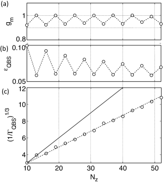
Figure 5: Theory versus numerical calculations: $N_{z}$ dependences of (a) peak conductance, (b) QBS energy and (c) QBS broadening parameter (both in units of $\gamma_{0}$). The numerical calculations were done for the resonance $(3,2)$ seen in FIG. 4(a). Our theory predicts roughly constant $g_{m}$, convergence of $\varepsilon_{QBS}$ to $\varepsilon_{\infty}$ and $\Gamma_{QBS}\sim N^{-3}_{z}$, all of which are consistent with numerical calculations. In panel (c), the solid curve has a slope of $\sim 0.3$ while the dashed curve has a slope of $\sim 0.2$. The dashed line is to guide the eye. Solid line shows results of theory and circles show results of numerical calculations.

IV.5 Role of Bearded Sites

Here we discuss the effect of bearded sites and show that they could lead to genuine bound states (i.e., vanishing $\Gamma_{QBS}$). For simplicity, we consider the rectangular-corner QPC with $N_{c}=1$ (FIG. 6). In the absence of bearded sites, the connecting bond would be a WCB. However, bearded sites transform an edge state initially located on the A- (B-) sublattice to edge state located on the B- (A-) sublattice Wakabayashi2001 , and thus turn a WCB into a SCB. Then, one can show that $C_{\tau}=0$ and then the level broadening vanishes, implying a pair of genuine bound states on this bond. Actually, bearded graphene is an insulatorWakabayashi2001 with a real band gap separating the edge states from the extended states. Thus, the $\rho_{0}$ vanishes at the QBS energy, which is consistent with vanishing $C_{\tau}$. The values of $B_{\tau}$ in the limit $N_{z}\rightarrow\infty$ are expected to be similar to those of the SCB $(N_{c}=3,i_{L}=2)$ in the same limit without bearded sites, because the wave functions in both cases are the same [Eq. (17)].

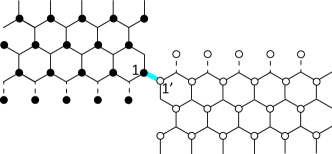
Figure 6: Bearded sites, represented by the circles attached to the dashed bonds, turn a WCB into a SCB. A pair of real bound states form on the bond (see text). Geometrically, the SCB (blue bond) shown here is similar to the SCB $(N_{c}=3,m=2)$ without bearded sites.

V Discussions

An essential element in the QBS theory presented above relates to the existence of non-bonding edge states at zero energy. Generically, such states are originated from the breaking of pseudo time-reversal symmetry, which is unique to the graphene lattice. Note that a perfect zigzag edge is not necessary for them to appear. Indeed, they could show up in graphene edges of almost any shape except for the perfect armchair one (in which case the symmetry is respected), even in the presence of a moderate external magnetic field Gusynin2009 . The observation makes our theory more widely applicable.

Because the QBS extends over only a few lattice constants, the Coulomb repulsion might be relatively strong. Assuming an on-site repulsion of $10~{}\mbox{eV}$ Wehling2011 , the repulsion between two electrons in QBS can be as large as $0.1~{}\mbox{eV}$, much bigger than that in conventional semiconductor quantum dots ($\sim\mbox{meV}$). These interactions serve to manipulate spins for possible applications in spintronics and qubits. For sufficiently wide samples, the QBS lifetime can be very long. As a result, charges may accumulate in the QPC and may give rise to dynamical Coulomb blockade effects Bulka2007 .

The QBS may be visualized using STM, which probes the dressed local density of states (LDOS) directly Tersoff1985 . One can show that in comparison with the bare LDOS, the dressed LDOS is enhanced by an amount $\delta\rho(\varepsilon_{F},\vec{r})\sim\frac{\Gamma_{QBS}}{(\varepsilon-\varepsilon_{QBS})^{2}+\Gamma^{2}_{QBS}}\cdot f(\vec{r}),$ where $f(\vec{r})$ is a function that decays as the STM tip moves away from a SCB by $|\vec{r}|$, as indicated in FIG. 3(c). The properties of the QBS can thus be directly determined.

The QBS can also have optical signatures. Specifically, we predict the optical absorption to be enhanced at the frequency $\nu\approx\frac{2\varepsilon_{\infty}}{h}$, which corresponds to the energy required to excite an electron from the lower QBS at $-\varepsilon_{\infty}$ to the upper one at $\varepsilon_{\infty}$. For $(N_{c}=3,m=2)$, this gives $\nu\approx 48\mbox{THz}$ in the infrared regime. Note that the QBS lifetime in this case is $\tau_{QBS}\approx 7\cdot\left(\frac{N_{z}}{100}\right)^{3}\mbox{ps}$, which can be much longer than the optical oscillation period $\nu^{-1}$. Thus, the system may be treated as an artificial two-level atom when dealing with its interaction with light at frequencies near or above $\nu$.

In addition, the QPCs can serve as the channel for a text-book single-level (and single-electron in the presence of Coulomb interactions) resonant tunneling transistor. Due to small level broadening, sharp turn-on can be expected at low temperatures.

VI Conclusion

In conclusion, we elucidated a mechanism for the formation of atomic bound states in a type of graphene QPCs. These states arise because of the zero energy edge states that are associated with the breaking of pseudo time-reversal symmetry. Their energies have been shown to be roughly independent of the sample dimensions. Finite level broadening exists, which shrinks to zero following a power law as the sample width increases. Because of the broadening, the states show up as Breit-Wigner resonances in the conductance of the QPCs. Such resonances dominate the electronic transport properties in the low energy regime.

K. W. acknowledges the financial support by Grant-in-Aid for Scientific Research from MEXT and JSPS (Nos. 25107005, 23310083 and 20001006). C. H. L. thanks the support from HK PolyU through grant No. G-YM41.

References

- (1) H. van Houten and Carlo Beenakker, Phys. Today 49, 22 (1996)
- (2) Y.-h. Zhang, P. Wahl and K. Kern, Nano Letters 11, 3838 (2011)
- (3) H. van Houten, C. W. J. Beenakker and B. J. van Wees, Semiconductors and Semimetals 35, 9 (1992)
- (4) Thomas Ihn, Semiconductor Nanostructures: Quantum States and Electronic Transport (Oxford University Press, 2010)
- (5) M. J. Iqbal, R. Levy, E. J. Koop, J. B. Dekker, J. P. de Jong, J. H. M. van der Velde, D. Reuter, A. D. Wieck, R. Aguado, Y. Meir and C. H. van der Wal, Nature 501, 79 (2013)
- (6) F. Bauer, J. Heyder, E. Schubert, D. Borowsky, D. Taubert, B. Bruognolo, D. Schuh, W. Wegscheider, J. von Delft and S. Ludwig, Nature 501, 73 (2013)
- (7) I. I. Yakimenko, V. S. Tsykunov and K.-F. Berggren, J. Phys.:Condens. Matter 25, 072201 (2013)
- (8) Y. Yoon, M.-G. Kang, P. Ivanushkin, L. Mourokh, T. Morimoto, N. Aoki, J. L. Reno, Y. Ochiai and J. P. Bird, Appl. Phys. Lett. 94, 213103 (2009)
- (9) T. Rejec and Y. Meir, Nature 442, 900 (2006)
- (10) K. Hirose, Y. Meir and N. S. Wingreen, Phys. Rev. Lett. 90, 026804 (2003)
- (11) K. J. Thomas, J. T. Nicholls, M. Y. Simmons, M. Pepper, D. R. Mace and D. A. Ritchie, Phys. Rev. Lett. 77, 135 (1996)
- (12) K. J. Thomas, J. T. Nicholls, N. J. Appleyard, M. Y. Simmons, M. Pepper, D. R. Mace, W. R. Tribe, and D. A. Ritchie, Phys. Rev. B 58, 4846 (1998)
- (13) A. K. Geim and K. S. Novoselov, Nat. Mater. 6, 183 (2007)
- (14) D. A. Areshkin and C. T. White, Nano Letters 7, 3253 (2007)
- (15) L. Tapasztó, G. Dobrik, P. Lambin, L. P. Biró Nature Nanotech., 3, 397 (2008)
- (16) A. Girdhar, C. Sathe, K. Schulten and J.-P. Leburton, PNAS 110, 16748 (2013).
- (17) J. Güttinger, F. Molotor, C. Stampfer, S. Schnex, A. jacobsen, S. Dröscher, T. Ihn and K. Ensslin, Rep. Prog. Phys. 75, 126502 (2012)
- (18) B. Özyilmaz, P. Jarillo-Herrero, D. Efetov and P. Kim, Appl. Phys. Lett. 91, 192107 (2007)
- (19) B. Terres, J. Dauber, C. Volk, S. Trellenkamp, U. Wichmann and C. Stampfer, Appl. Phys. Lett. 98, 032109 (2011)
- (20) M. Y. Han, J. C. Brant and P. Kim, Phys. Rev. Lett. 104, 056801 (2010)
- (21) C. Stampfer, E. Schurtenberger, F. Molitor, J. Güttinger, T. Ihn and K. Ensslin, Int. J. Mod. B 23, 2647 (2009)
- (22) P. Darancet, V. Olevano and D. Mayou, Phys. Rev. Lett. 102, 136803 (2009)
- (23) K. Todd, H.-T. Chou, A. Amasha and D. Goldhaber-Gordon, Nano Letters 9, 416 (2009)
- (24) M. Fujita, K. Wakabayashi, K. Nakada and K. Kusakabe, J. Phys. Soc. Jpn. 65, 1920 (1996)
- (25) K. Nakada, M. Fujita, G. Dresselhaus and M. S. Dresselhaus, Phys. Rev. B 54, 17954 (1996)
- (26) T. Enoki, Phys. Scr. T146, 014008 (2012)
- (27) K. Wakabayashi and S. Dutta, Solid State Comm. 152, 1420 (2012)
- (28) H. Karimi and I. Affleck, Phys. Rev. B 86, 115446 (2012)
- (29) A. Rycerz, J. Tworzydlo and C. W. J. Bennakker, Nat. Phys. 3, 172 (2007)
- (30) K. Wakabayashi, Y. Takane and M. Sigrist, Phys. Rev. Lett. 99, 036601 (2007)
- (31) D. Gunlycke, J. Li, J. W. Mintmire and C. T. White, Nano Letters 10, 3638 (2010)
- (32) J. Guo, D. Gunlycke and C. T. White, Appl. Phys. Lett. 92, 163109 (2008)
- (33) D. Gunlecke, D. A. Areshkin, J. Li, J. W. Mintmire and C. T. White, Nano Letters 7, 3608 (2007)
- (34) K. Wakabayashi and T. Aoki, Int. J. Mod. Phys. B 16, 4897 (2002)
- (35) A. R. Akhmerov, J. H. Bardarson, A. Rycerz and C. W. J. Beenakker, Phys. Rev. B 77, 205416 (2008)
- (36) H.-Y. Deng, K. Wakabayashi and C.-H. Lam, J. Phys. Soc. Jpn. 82, 104707 (2013)
- (37) E. N. Economou, Green’s functions in Quantum Physics (Springer-Verlag, 1979)
- (38) Employing the same approximations, we can derive from Eq.(4) that , where and . We note that for energies close to zero, because of the particle-hole symmetry. Thus, is much smaller than .
- (39) Contributions from the high-energy sector (consisting of short transverse wave-length modes) are vanishingly small due to particle-hole symmetry. The low-energy section consisting of long-wavelength modes contribute less and less as increases, since the wave functions scale as near edges. Actually, the transverse wave functions of such modes are sine waves (See Wakabayashi2012 ).
- (40) Y. Shimomura, Y. Takane and K. Wakabayashi, J. Phys. Soc. Jpn. 80, 054710 (2011)
- (41) In Eq. (16), the factor accounts for the fact that of the two degenerate sets of the edge modes obtained in the semi-infinite limit, only one contributes near either edge.
- (42) We see that the decreases with . For our assumption to hold, we must have . Note that , from which we infer that the widest possible ribbon should not exceed , i.e., around . If indeed exceeds this critical value, one can show that Eq. (18) still holds but the coefficient has to sum over more channels and subsequently, the scales as instead of (The additional factor accounts for the number of dispersive bands).
- (43) K. Wakabayashi, Phys. Rev. B 64, 125428 (2001)
- (44) H. A. Bethe, Phys. Rev. 66, 163 (1944)
- (45) J. Bardeen, Phys. Rev. Lett. 6, 57 (1961)
- (46) U. Fano, Phys. Rev. 124, 1866 (1961)
- (47) T. O. Wehling, E. Sasioglu, C. Friedrich, A. I. Lichtenstein, M. I. Katsnelson and S. Blügel, Phys. Rev. Lett. 106, 236805 (2011)
- (48) V. P. Gusynin, V. A. Miransky, S. G. Sharapov, I. A. Shovkovy and C. M. Wyenberg, Phys. Rev. B 79, 115431 (2009)
- (49) B. R. Bulka, T. Kostyrko, M. Tolea and I. V. Dinu, J. Phys.: Condens. Matter 19, 255211 (2007)
- (50) J. Tersoff and D. R. Hamann, Phys. Rev. B 31, 805 (1985)