Convergence of empirical distributions in an
interpretation of quantum mechanics

Abstract

From its beginning, there have been attempts by physicists to formulate quantum mechanics without requiring the use of wave functions. An interesting recent approach takes the point of view that quantum effects arise solely from the interaction of finitely many classical “worlds.” The wave function is then recovered (as a secondary object) from observations of particles in these worlds, without knowing the world from which any particular observation originates. Hall, Deckert and Wiseman [Physical Review X 4 (2014) 041013] have introduced an explicit many-interacting-worlds harmonic oscillator model to provide support for this approach. In this note we provide a proof of their claim that the particle configuration is asymptotically Gaussian, thus matching the stationary ground-state solution of Schrödinger’s equation when the number of worlds goes to infinity. We also construct a Markov chain based on resampling from the particle configuration and show that it converges to an Ornstein–Uhlenbeck process, matching the time-dependent solution as well.

1 Introduction

Let $x_{1},\ldots,x_{N}$ be a finite sequence of real numbers satisfying the recursion relation

$$x_{n+1}=x_{n}-{1\over x_{1}+\ldots+x_{n}}.$$ (1.1)

In this note we show that for a certain class of solutions (monotonic with zero-mean), the empirical distribution of the $x_{n}$ converges to standard Gaussian as $N\to\infty$. We also construct a simple Markov chain based on resampling from this empirical distribution and show that it converges to an Ornstein–Uhlenbeck process.

Hall et al. (2014) derived the recursion relation (1.1) via Hamiltonian mechanics and used it to justify a novel interpretation of quantum mechanics. The solution they considered represents the stationary ground-state configuration of a harmonic oscillator in $N$ “worlds,” where $x_{n}$ is the location (expressed in dimensionless units) of a particle in the $n$th world. The particles behave classically (deterministically in accordance with Newtonian mechanics) within each world, and there is a mutually repulsive force between particles in adjacent worlds. Observers have access to draws from the empirical distribution

$$\mathbb{P}_{N}(A)={\#\{n\colon x_{n}\in A\}\over N}$$

for any Borel set $A\subset\mathbb{R}$, but do not know the world from which any observation originates due to their ignorance as to which world they occupy. In statistical language, Efron’s nonparametric bootstrap can be used by observers (to obtain draws with replacement from the whole configuration $\{x_{1},\ldots,x_{N}\}$), but they are unable to identify any particular $x_{n}$.

Hall et al. (2014) discovered that $\mathbb{P}_{N}$ is approximately Gaussian, thus corresponding to the stationary ground-state solution of Schrödinger’s equation for the wave function of a particle in a parabolic potential well, and furnishing a many-interacting-worlds interpretation of this wave function. They provided convincing numerical evidence that the Gaussian approximation is accurate when $N=11$, a case in which the recursion relation admits an exact solution. As far as we know, however, a formal proof of convergence is not yet available. Sebens (2014) independently proposed a similar many-interacting-worlds interpretation, called Newtonian quantum mechanics, although no explicit example was provided. Our interest in studying the explicit model (1.1) is that rigorous investigation of its limiting behavior becomes feasible. Both Hall et al. (2014) and Sebens (2014) noted the ontological difficulty of a continuum of worlds, a feature of an earlier but closely related hydrodynamical approach due to Holland (2005), Poirier (2010) and Schiff and Poirier (2012).

The motivation for the recursion (1.1) given by Hall et al. (2014) was to explore explicitly the consequences of replacing the continuum of fluid elements in the Holland–Poirier theory by a “huge” but nevertheless finite number of interacting worlds. Yet their approach raises the question of whether such a discrete model has a stable solution when the number of worlds becomes large. A formal way to address this question is to establish the convergence of $\mathbb{P}_{N}$ under suitable conditions. The problem is non-trivial, however, because explicit solutions of the recursion are only available for small values of $N$, and numerical methods are useful only for exploratory purposes. Nevertheless, we are able to establish our result using only standard methods of distribution theory, and most crucially the Helly selection theorem. In addition, by making use of Stein’s method, we are able to find a rate of convergence. We further construct a Markov chain based on bootstrap resampling from $\mathbb{P}_{N}$ and show that it converges to the Ornstein–Uhlenbeck process corresponding to the full (time-dependent) ground-state solution of Schrödinger’s equation in this setting.

Our main results are collected in Section 2, and their proofs are in Section 3. For general background on parallel-world theories in quantum physics, we refer the interested reader to the book of Greene (2011). For the convenience of the reader, at the end of Section 3 we have provided Hall et al. (2014)’s derivation of (1.1) as representing a ground state solution of the many-interacting-worlds Hamiltonian.

2 Main results

Our main result is that $\mathbb{P}_{N}$ has a standard Gaussian limit for monotonic zero-mean solutions $\{x_{1},\ldots,x_{N}\}$ to the recursion (1.1). Monotonicity and zero-mean (along with the recursion) are necessary conditions for a ground-state solution of the many-interacting-worlds Hamiltonian, so our result establishes in full generality the normal approximation claimed by Hall et al. (2014). We also show that such solutions to the recursion exist and are unique for each $N\geq 3$ (Lemma 1 in Section 3). The solutions are indexed by $N$, and for clarity in the proofs we will write $x_{n}$ as $x_{N,n}$. For now, though, we suppress the dependence on $N$. Our main result is as follows.

Theorem 1.

The unique monotonic zero-mean solution $\{x_{n},n=1,\ldots,N\}$ of the recursion relation (1.1) satisfies $\mathbb{P}_{N}\stackrel{{\scriptstyle d}}{{\longrightarrow}}{\cal N}(0,1)$ as $N\to\infty$.

Remarks

1. Our proof of Theorem 1 will proceed by showing that $\mathbb{P}_{N}$ is close in distribution to a certain piecewise-constant density $y_{N}(x)$, which in turn is shown to converge pointwise to the ${\cal N}(0,1)$ density. Further, we will construct a coupling between two random variables $X_{N}\sim\mathbb{P}_{N}$ and $\tilde{X}_{N}\sim y_{N}$ such that $|X_{N}-\tilde{X}_{N}|\to 0$ almost surely, so the result will then follow from Slutsky’s lemma. An illustration of $y_{N}(x)$ is given in Fig. 1.

2. Stein’s method, as often used for studying normal approximations to sums of independent random variables (see Chen et al., 2010), is applicable in our setting and gives insight into the rate of convergence. We will discuss this approach following the proof. Stein’s method becomes particularly easy to apply in our setting because $y_{N}(x)$ is the so-called zero-bias density of $\mathbb{P}_{N}$.

3. Let $w_{1},\ldots,w_{N}$ satisfy the more general recursion relation

   $$w_{n+1}=w_{n}-{\sigma^{2}\over w_{1}+\ldots+w_{n}},$$

   where $\sigma^{2}>0$. The scaled sequence $x_{n}=w_{n}/\sigma$ satisfies (1.1), so Theorem 1 applies and the empirical distribution of $\{w_{1},\ldots,w_{N}\}$ converges to ${\cal N}(0,\sigma^{2})$. It is striking that the variance $\sigma^{2}$, rather than the standard deviation, appears linearly in the recursion for $w_{n}$. For the harmonic oscillator studied by Hall et al. (2014), $\sigma^{2}=\hbar/(2m\omega)$, where $\hbar$ is the reduced Planck constant, $m$ is the mass of the particle, and $\omega$ is the angular frequency.

4. Monotonicity of the solution to the recursion may not be necessary, even though our proof of Theorem 1 relies on it. We have found from numerical experiments that non-monotonic solutions can exist with $\mathbb{P}_{N}$ indistinguishable from standard Gaussian. From the physical point of view, however, monotonicity is an essential requirement: the ordering of the particles is always preserved by the repulsive nature of the interaction between worlds (Hall et al. 2014, Section III).

5. Theorem 1 is equivalent to the statement that if $n=n(N)\to\infty$ with $n/N\to\alpha$ for some $0<\alpha<1$, then $x_{n}$ converges to the upper-$\alpha$-quantile of ${\cal N}(0,1)$. This implies a simple recursion approximation for intermediate normal quantile.

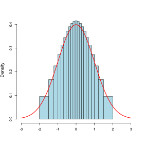
Figure 1: Harmonic oscillator ground state configuration for $N=22$ worlds compared with the ${\cal N}(0,1)$ density. The histogram is the $\mathbb{P}_{N}$-zero-bias density $y_{N}(x)$, and the breaks in the histogram are successive $x_{n}$.

Numerical example

The recursion can be rapidly iterated, but to generate an exact monotonic zero-mean solution, $x_{1}$ needs to be known. A “randomly chosen” initial point will not lead to a solution, and the system is non-robust to the choice of $x_{1}$, which parallels the physics in the sense that explicit ground-state solutions of the many-interacting-worlds Hamiltonian are not available.

We consider an example with $N=22$ worlds, and use the following trial-and-error approach to obtain an approximate solution. Given the proximity of $x_{n}$ to normal quantiles noted above, the $1/N$-upper-quantile of ${\cal N}(0,1)$ might be considered as a suitable initial choice of $x_{1}$. From our numerical experiments, however, we have found that the $1/(2N)$-upper-quantile (denoted $q_{N}$) is much more accurate; the normal approximation is poor in the extreme tail of $\mathbb{P}_{N}$ (i.e., more extreme than $\pm x_{1}$), and the scaling by 2 compensates well for this. A search over a fine grid in a small neighborhood of $q_{N}$ then quickly yields a very accurate solution by minimizing $|x_{1}+x_{N}|$. In this example, $q_{N}=2.0004$ and the best approximation is $x_{1}=2.0025$ (to 4 decimal places).

Fig. 1 displays the $\mathbb{P}_{N}$-zero-bias density $y_{N}(x)$ having mass $1/(N-1)$ uniformly distributed over the intervals between successive $x_{n}$, along with the ${\cal N}(0,1)$ density. The approximation is remarkably good except around zero and in the extreme tails.

General solutions to the quantum harmonic oscillator

Using an approach to quantum mechanics pioneered by Edward Nelson, it can be shown that the full ground state solution of Schrödinger’s equation for a harmonic oscillator can be represented in terms of the distribution of an Ornstein–Uhlenbeck (OU) process. Moreover, the complete family of solutions can be represented by adding this ground-state process to all solutions of the classical harmonic oscillator; see, e.g., Paul and Baschnagel (2013), pages 122–124. The limit in Theorem 1 refers to the stationary distribution of this ground-state OU process, but it is also possible to construct a many-interacting-worlds approximation to the OU process itself. This can be done in terms of simple random samples from $\mathbb{P}_{N}$ that evolve as a Markov chain, as we now explain.

Let $\{Z_{1},\ldots,Z_{m}\}$ be an independent random sample of size $m$ from ${\cal N}(0,1)$, corresponding to $m$ draws from $\mathbb{P}_{N}$ in the limit as $N\to\infty$ (by Theorem 1). Let $Y_{0}=\sum_{i=1}^{m}Z_{i}$, and let $Y_{1}$ be obtained from $Y_{0}$ by replacing a randomly selected $Z_{i}$ by an independent draw from ${\cal N}(0,1)$. By iterating this “random single replacement” mechanism (cf. sequential bootstrap), we obtain a stationary Markov chain of samples of size $m$, and an autoregressive Gaussian time series $Y_{k}$ satisfying

$$Y_{k}=(1-\lambda)Y_{k-1}+\epsilon_{k},\ \ k=1,2,\ldots$$

where $\lambda=\lambda_{m}=1/m$, and the innovations $\epsilon_{k}\sim{\cal N}(0,2-\lambda)$ are independent of each other and of past values of the time series (cf. Chen et al., 2010, pages 22–25). Construct a rescaled version of the time series as a random element of the Skorohod space $D[0,\infty)$ by setting

$$X_{t}^{(m)}=Y_{[mt]}/\sqrt{m},\ \ t\geq 0,$$

where $[\cdot]$ is the integer part. Using a result of Phillips (1987) concerning first-order autoregressions with a root near unity, we can show that $X_{t}^{(m)}$ converges in distribution as $m\to\infty$ to the (stationary) OU process $X_{t}$ that satisfies the stochastic differential equation

$$dX_{t}=-X_{t}\,dt+\sqrt{2}\,dW_{t},\ \ t\geq 0,$$

where $W_{t}$ is a standard Wiener process and $X_{0}\sim{\cal N}(0,1)$. It suffices to consider the time series

$$y_{k}=Y_{k}/\sqrt{1-\lambda/2},\ \ k=1,2,\ldots,$$

which has iid-${\cal N}(0,2)$ innovations and autoregressive parameter $a=(1-\lambda)/\sqrt{1-\lambda/2}$. Setting $a=e^{c/T}$ where $c=-1$ and $T=T_{m}\to\infty$ to match Phillips’s notation, we have $T/m\to 1$, so his Lemma 1 (a) gives that the process $y_{[mt]}/\sqrt{m}$ converges in distribution to the OU process $X_{t}$, as required.

We expect the same limit result if the Markov chain consists of random samples of size $m$ from $\mathbb{P}_{N}$ (that evolve by the same mechanism), provided $N$ and $m$ simultaneously tend to infinity. The proof of such a general result would be difficult, however, as it would involve extending the above argument to time series in which the innovations depend on $m$ and $N$ and that are no longer independent. Nevertheless, we can show that such a result holds provided $m=m_{N}\to\infty$ slowly enough, as follows.

Theorem 2.

Suppose the conditions of Theorem 1 hold. Let $Y_{N,k}$ be the sum of values at time $k$ of the stationary Markov chain of samples of size $m$ generated by the mechanism of random single replacement from $\mathbb{P}_{N}$. Then, if $m=m_{N}\to\infty$ and $m=o({\log N})^{1/3}$ the rescaled process

$$\hbox{\vbox{\hrule height=0.5pt\kern 1.29167pt\hbox{\kern-1.00006pt$X$\kern-1.00006pt}}}_{t}=Y_{N,[mt]}/\sqrt{m},\ \ t\geq 0$$

converges in distribution on $D[0,\infty)$ to the OU process $X_{t}$.

3 Proofs

Before proceeding to the proof of Theorem 1, we state a lemma (to be proved later) that gives the key properties needed to establish the theorem, and also establishes the existence of a unique solution to the recursion relation that satisfies the conditions of the theorem. Throughout we implicitly assume $N\geq 3$. We will also make extensive use of the notion of zero-median in the following sense: if $N$ is odd, then $x_{(N+1)/2}=0$; if $N$ is even, then $x_{N/2}=-x_{(N/2)+1}$.

Lemma 1.

Every zero-median solution $x_{1},\ldots,x_{N}$ of (1.1) satisfies the following properties:

• • Zero-mean: $x_{1}+\ldots+x_{N}=0$.

  • Variance-bound: $x_{1}^{2}+\ldots+x_{N}^{2}=N-1$.

  • Symmetry: $x_{n}=-x_{N+1-n}$ for $n=1,\ldots,N$.

Further, there is a unique solution $x_{1},\ldots,x_{N}$ of (1.1) such that (P1) and

• • Strictly decreasing: $x_{1}>\ldots>x_{N}$

hold. This solution has the zero-median property, and thus also satisfies (P2) and (P3).

Without loss of generality we can assume that (P4) holds, since if we start with an increasing zero-median solution, reversing the order of the solution provides a decreasing solution by (P3), and any monotonic solution is strictly monotonic. The dependence on $N$ is now made explicit: write $x_{n}=x_{N,n}$, and also denote $S_{N,n}=x_{N,1}+\ldots+x_{N,n}$ for $n=1,\ldots,N$.

First we show that $x_{N,1}\geq\sqrt{\log N}/2$. For odd $N$, the median $x_{N,m}=0$, where $m=m_{N}=(N+1)/2$, and the telescoping sum

$$x_{N,1}=\sum_{n=1}^{m-1}(x_{N,n}-x_{N,n+1})>{1\over x_{N,1}}\sum_{n=1}^{m-1}{1\over n}>{\log m\over x_{N,1}}.$$

Here we used (1.1), (P4) and $S_{N,n}<nx_{N,1}$ for the first inequality, and Euler’s approximation to the partial sums of the harmonic series for the second inequality. This gives $x_{N,1}>\sqrt{\log m}$, and a similar argument shows that the same is true for $N$ even with $m=N/2$. The claim then follows using the inequality $\log(N/2)>(\log N)/4$ for $N\geq 3$.

Now using the symmetry property to bound $S_{N,n}$ from below by $x_{N,1}$ for $n=1,\ldots,N-1$, the recursion (1.1) gives the uniform bound

$$0<x_{N,n}-x_{N,n+1}=1/S_{N,n}\leq 1/x_{N,1},$$

and an upper bound on the mesh of the sequence:

$$\delta_{N}\equiv\max_{n=1,\ldots,N-1}|x_{N,n}-x_{N,n+1}|\leq 2/\sqrt{\log N}.$$ (3.1)

Next, for $x\in\mathbb{R}$ such that $|x|<x_{N,1}$, let $n=n(x,N)$ be the unique index satisfying $x_{N,n+1}\leq x<x_{N,n}$, and define $y_{N}(x)=S_{N,n}/(N-1)$, so from the recursion relation (1.1) we have

$$y_{N}(x)=[(N-1)(x_{N,n}-x_{N,n+1})]^{-1}.$$ (3.2)

Defining $y_{N}(x)=0$ for $|x|\geq x_{N,1}$ makes $y_{N}$ into a piecewise-constant density; see Fig. 1 for an illustration.

We will show that $y_{N}(x)$ converges uniformly in $x$, although we only need pointwise convergence. Let $X_{N}$ be a random variable distributed according to the empirical distribution $\mathbb{P}_{N}$ that was defined in the Introduction. Set $Y_{N}(x)=X_{N}I(X_{N}>x)$. Since $y_{N}(x)=(N/(N-1))EY_{N}(x)$, it suffices to consider $EY_{N}(x)$. We use a subsequence argument. Note that $X_{N}$ has second moment $1-1/N$ by (P2), so it is bounded in probability (tight). Thus, by the Helly selection theorem, there is a subsequence that converges in distribution. Let $D\subset\mathbb{R}$ denote the set of continuity points of the limit distribution. For $x\in D$, note that $Y_{N}(x)$ converges in distribution (along the subsequence) by the continuous mapping theorem. Thus, since $Y_{N}(x)$ is uniformly integrable as the second moment $EY_{N}^{2}(x)\leq EX_{N}^{2}$ is uniformly bounded by (P2), we obtain that $y_{N}(x)$ has a pointwise limit for all $x\in D$.

Below we will show that there is a unique continuous function $y(x)$ such that $y_{N}(x)\to y(x)$ for all $x\in D$. Then, using the monotonicity of $y_{N}(x)$ over either $x\geq 0$ or $x\leq 0$, the whole sequence $y_{N}(x)$ must converge pointwise to $y(x)$ for all $x\in\mathbb{R}$. The functions $y_{N}(x)$ are right-continuous, so, by the same argument that is used to prove the Glivenko–Cantelli theorem and using the continuity of $y(x)$, we will also then have uniform convergence $y_{N}(x)\to y(x)$ for $x\in\mathbb{R}$, as claimed.

We have shown that $y(x)=\lim_{N\to\infty}y_{N}(x)$ exists for $x\in D$ (a dense subset of $\mathbb{R}$), when the limit is taken over a subsequence of $y_{N}$. Now extend the definition of $y(x)$ to a general $x\in\mathbb{R}$ by taking a sequence $z_{r}\in D$ such that $z_{r}\downarrow x$ and setting $y(x)\equiv\lim_{r\to\infty}y(z_{r})$ . Since $y(x)$ shares the same monotonicity properties as the limit of $y_{N}(x)$ on $x\in D$, it is well-defined, i.e., not dependent on the choice of the sequence $z_{r}$. Note that $y(x)$ is right-continuous (by construction), and $y_{N}(x)\to y(x)$ for all $x\in\mathbb{R}$ at which $y(x)$ is continuous. In particular, $y_{N}(x)\to y(x)$ a.e. $[dx]$, since $y(x)$ has at most countably many discontinuities.

From the recursion relation (1.1) we have

$${y_{N}(x_{N,n+1})-y_{N}(x_{N,n})\over x_{N,n+1}-x_{N,n}}={x_{N,n+1}/(N-1)\over-S_{N,n}^{-1}}={x_{N,n}-S_{N,n}^{-1}\over-S_{N,n}^{-1}(N-1)}={1\over N-1}-x_{N,n}y_{N}(x_{N,n}).$$

Let $0\leq u<v$ be continuity points of $x\mapsto y(x)$, and take $N$ to be sufficiently large that $x_{N,1}>v$, so $n(v,N)$ and $n(u,N)$ are defined. Multiply the first and last parts of the above display by $x_{N,n+1}-x_{N,n}$ and sum over $n$ from $n(v,N)$ to $n(u,N)$, to obtain an equation of the form $A_{N}=B_{N}-C_{N}$. Here $A_{N}$ and $B_{N}$ are telescoping sums:

$$A_{N}=y_{N}(u)-y_{N}(v)\to y(u)-y(v),\ \ B_{N}=(u_{N}-v_{N})/(N-1)\to 0,$$

where $u_{N}=x_{N,n(u,N)}$, $v_{N}=x_{N,n(v,N)}$, and

$$C_{N}=\int_{u_{N}}^{v_{N}}h_{N}(x)y_{N}(x)\,dx,$$

where $h_{N}(x)\equiv x_{N,n(x,N)}$. Note that by (3.1) we have $h_{N}(x)\to x$ for all $x\in\mathbb{R}$. This leads to the integral equation

$$y(u)-y(v)=-\int_{u}^{v}xy(x)\,dx$$

by applying the bounded convergence theorem, since $h_{N}(x)y_{N}(x)\to xy(x)$ a.e. $[dx]$; note that the $y_{N}(x)$ are uniformly bounded, since they are nonnegative, unimodal, and converge pointwise. Moreover, by the right-continuity of $y(x)$, the integral equation holds for all $0\leq u<v$, and, by the symmetry property the case $u<v\leq 0$ is also covered by the above argument. Therefore $y(x)$ is differentiable and satisfies the linear first-order ODE $y^{\prime}(x)+xy(x)=0$. This ODE has general solution of the form $y(x)=c\,\varphi(x)$, where $c$ is a constant and $\varphi(x)$ is the standard normal density.

It remains to identify $c$. By (3.2),

$$\int_{-\infty}^{\infty}y_{N}(x)\,dx=\sum_{n=1}^{N-1}[(N-1)(x_{N,n}-x_{N,n+1})]^{-1}(x_{N,n}-x_{N,n+1})=1,$$ (3.3)

so by Fatou’s lemma (applicable since $0\leq y_{N}(x)\to y(x)$ a.e.)

$$c=\int_{-\infty}^{\infty}y(x)\,dx\leq\liminf_{N\to\infty}\int_{-\infty}^{\infty}y_{N}(x)\,dx=1.$$

Let $\tilde{X}_{N}$ be a random variable having density $y_{N}(x)$. The second moment of $\tilde{X}_{N}$

$$\int_{-\infty}^{\infty}x^{2}\,y_{N}(x)\,dx = \sum_{n=1}^{N-1}[(N-1)(x_{N,n}-x_{N,n+1})]^{-1}(x_{N,n}^{3}-x_{N,n+1}^{3})/3$$

$$\leq (N-1)^{-1}\sum_{n=1}^{N-1}x_{N,n}^{2}\leq 1,$$

where the last inequality follows from the variance bound (P2) in Lemma 1. This implies that the $\tilde{X}_{N}$ are tight, so for any $\epsilon>0$ there exist $u<v$ such that $\int_{u}^{v}y_{N}(x)\,dx>1-\epsilon$ for all $N$. By the bounded convergence theorem,

$$\int_{u}^{v}y_{N}(x)\,dx\to\int_{u}^{v}y(x)\,dx=c\int_{u}^{v}\varphi(x)\,dx,$$

so $\int_{u}^{v}y_{N}(x)\,dx<c+\epsilon$ for $N$ sufficiently large. This shows that $c>1-2\epsilon$, but as $\epsilon>0$ was arbitrary and $c\leq 1$, we have established that $c=1$.

This uniquely identifies the function $y(x)$ as $\varphi(x)$, so we have shown that $y_{N}(x)\to y(x)=\varphi(x)$ for all $x\in\mathbb{R}$. Hence the distribution of $\tilde{X}_{N}$ (having density $\tilde{p}_{N}$) converges in total variation distance (and consequently in distribution) to ${\cal N}(0,1)$. The last part of the proof shows that it is possible to create a coupling between $X_{N}\sim\mathbb{P}_{N}$ and $\tilde{X}_{N}$ (on the same probability space) such that

$$|X_{N}-\tilde{X}_{N}|\leq|x_{N,n}-x_{N,n+1}|\hbox{ when }\tilde{X}_{N}\in[x_{N,n+1},x_{N,n}].$$ (3.4)

We then have the uniform bound

$$|X_{N}-\tilde{X}_{N}|\leq\max_{n=1,\ldots,N-1}|x_{N,n}-x_{N,n+1}|=\delta_{N}\to 0$$ (3.5)

using (3.1), so by Slutsky’s lemma we conclude that $\mathbb{P}_{N}$ converges in distribution to ${\cal N}(0,1)$.

To create the above coupling between $X_{N}$ and $\tilde{X}_{N}$, note that $\tilde{X}_{N}$ uniformly distributes mass $1/(N-1)$ on each interval between successive $x_{N,n}$. Let $N$ be odd (a similar argument works for $N$ even), in which case $x_{N,m}=0$ for $m=(N+1)/2$. We need to split each interval in such a way that there is mass $1/N$ assigned to $x_{N,n}$ from the two adjacent parts (or the one adjacent part if $n=1$ or $N$). This can be done as follows. Split the first interval to the right of zero so there is mass $L_{1}=1/(2N)$ on the left part and $R_{1}=1/(N-1)-1/(2N)$ on the right part. Split the $j$-th interval to the right of zero so there is mass $L_{j}=(2j-1)/(2N)-(j-1)/(N-1)$ on the left part, and $R_{j}=1/(N-1)-L_{j}=j/(N-1)-(2j-1)/(2N)$ on the right part, for $j=2,\ldots,(N-1)/2$. Some algebra shows that the mass assigned the right endpoint of the $j$-th interval is $R_{j}+L_{j+1}=1/N$ for $j=1,\ldots,(N-1)/2-1$, and for the last interval ($j=(N-1)/2$) it is also $1/N$. Use symmetry to define the coupling over the negative intervals. Note that the median $x_{N,m}=0$ gets mass $1/((2N)+1/((2N)=1/N$ as well. This completes the proof of Theorem 1. ∎

Application of Stein’s method

Stein’s method allows us to obtain bounds on the rate of convergence. The rate will be measured using Wasserstein distance: for two probability distributions $\mu$ and $\nu$ on $\mathbb{R}$,

$$d_{W}(\mu,\nu)=\sup_{h\in{\cal L}}|Eh(X)-Eh(Y)|$$

where $X\sim\mu$ and $Y\sim\nu$, and $\cal L$ is the collection of 1-Lipschitz functions $h\colon\mathbb{R}\to\mathbb{R}$ such that $|h(x)-h(y)|\leq|x-y|$. Here we derive bounds on $d_{W}(\mathbb{P}_{N},{\cal N})$, where $\cal N$ is Gaussian with the same mean and variance as $\mathbb{P}_{N}$.

Goldstein and Reinert (1997) introduced the notion of zero-bias distributions, defined as follows. Given a r.v. $X$ with mean zero and variance $\sigma^{2}$, there is a r.v. $X^{*}$ such that $\sigma^{2}E[f^{\prime}(X^{*})]=E[Xf(X)]$ for all absolutely continuous functions $f\colon\mathbb{R}\to\mathbb{R}$ for which $E|Xf(X)|<\infty$. (This result also appears as Proposition 2.1 of Chen et al. (2010), although a slight correction is needed: the $\sigma^{2}$ is misplaced in the first display).

The distribution of $X^{*}$ is the $X$-zero-bias distribution. It has density $p^{*}(x)=E[XI(X>x)]/\sigma^{2}$. The unique fixed point of the zero-bias transformation is ${\cal N}(0,\sigma^{2})$, and the intuition behind Stein’s method is that if $X$ is close to $X^{*}$ it should be close in distribution to ${\cal N}(0,\sigma^{2})$. Indeed, from Lemma 2.1 of Goldstein (2004), the Wasserstein distance between $X$ and a normal variable having the same mean and variance is bounded above by $2E|X-X^{*}|$ when $X$ and $X^{*}$ are defined on the same probability space.

In our setting, $\tilde{X}_{N}$ has the $X_{N}$-zero-bias distribution because its density $y_{N}(x)$ agrees with $p^{*}(x)$ when $X=X_{N}$. Further, we have coupled $\tilde{X}_{N}$ and $X_{N}$ to satisfy (3.4). Thus

$$d_{W}(\mathbb{P}_{N},{\cal N})\leq 2E|X_{N}-\tilde{X}_{N}|\leq{2\over N-1}\sum_{n=1}^{N-1}(x_{N,n}-x_{N,n+1})={4x_{N,1}\over N-1}.$$ (3.6)

Larry Goldstein pointed out that it is possible to obtain a lower bound on the Wasserstein distance between $\mathbb{P}_{N}$ and its zero-bias distribution as follows. Consider the “sawtooth” piecewise linear function $h\colon\mathbb{R}\to\mathbb{R}$ defined to have knots at each $x_{n}$ and at each midpoint $m_{n}=(x_{n}+x_{n+1})/2$ between successive $x_{n}$, such that $h(x_{n})=0$ and $h(m_{n})=(x_{n}-x_{n+1})/2$, with $h$ vanishing outside $[x_{N},x_{1}]$. Clearly $h$ is 1-Lipschitz and $Eh(X_{N})=0$, so from its definition the Wasserstein distance between $\mathbb{P}_{N}$ and its zero-bias distribution is bounded below by $Eh(\tilde{X}_{N})=x_{N,1}/[2(N-1)]$, which is of the same order as the upper bound on $d_{W}(\mathbb{P}_{N},{\cal N})$.

This strongly suggests $d_{W}(\mathbb{P}_{N},{\cal N})\asymp x_{N,1}/N$. Moreover, as mentioned earlier, there is convincing numerical evidence that $x_{N,1}\asymp q_{N}$, where $q_{N}$ is the upper $1/(2N)$-quantile of ${\cal N}(0,1)$. Indeed, we have already shown $x_{N,1}\geq\sqrt{\log N}/2$, and using Mills ratio it can be shown that $q_{N}\asymp\sqrt{\log N}$, so combining with (3.6) we expect $d_{W}(\mathbb{P}_{N},{\cal N})\asymp\sqrt{\log N}/N$. In terms of what we have actually proved, however, the uniform coupling property (3.5) and (3.1) only give the weaker upper bound $d_{W}(\mathbb{P}_{N},{\cal N})\leq 2\delta_{N}\leq 4/\sqrt{\log N}.$

Proof of Theorem 2

We have already shown that $X_{t}^{(m)}$ converges in distribution to the OU process $X_{t}$. By appealing to Slutsky’s lemma for random elements of metric spaces (van der Vaart, 2000, Theorem 18.10), it thus suffices to show that for each $T>0$ the processes $\{\hbox{\vbox{\hrule height=0.5pt\kern 1.29167pt\hbox{\kern-1.00006pt$X$\kern-1.00006pt}}}_{t},t\in[0,T]\}$ and $\{X_{t}^{(m)},t\in[0,T]\}$ can be coupled as random elements of $D[0,T]$ on a joint probability space, with their difference tending uniformly to zero in probability. The upper bound on the Wasserstein distance just derived implies that if $X_{N}\sim\mathbb{P}_{N}$, there exists $Z\sim{\cal N}(0,1)$ on a joint probability space with $E|X_{N}-Z|=O(1/\sqrt{\log N})$.

Further, any sequence of iid-$\mathbb{P}_{N}$ r.v.s can be coupled in this way using independent coupled pairs on a joint probability space. The single replacement mechanism that generates samples of size $m$ from $\mathbb{P}_{N}$ can be coupled with a chain of samples from ${\cal N}(0,1)$ by using the same randomly selected index in each transition. Each transition involves selecting the update from an independent sample of size $m$, so $m([mT]+1)$ coupled pairs are involved over the interval $[0,T]$. Thus we have constructed a coupling of the processes $\hbox{\vbox{\hrule height=0.5pt\kern 1.29167pt\hbox{\kern-1.00006pt$X$\kern-1.00006pt}}}_{t}$ and $X_{t}^{(m)}$ over $t\in[0,T]$ with

$$E\bigg{\{}\sup_{t\in[0,T]}|\hbox{\vbox{\hrule height=0.5pt\kern 1.29167pt\hbox{\kern-1.00006pt$X$\kern-1.00006pt}}}_{t}-X_{t}^{(m)}|\bigg{\}}\leq m([mT]+1)E|X_{N}-Z|/\sqrt{m}=m^{3/2}O(1/\sqrt{\log N})\to 0$$

since we have assumed $m=o({\log N})^{1/3}$, so the result follows by Chebyshev’s inequality. ∎

Proof of Lemma 1

The following result is needed to prove Lemma 1. Denote $m=m_{N}=(N+1)/2$ if $N$ is odd and $m=m_{N}=N/2$ if $N$ is even. For any given $x_{1}>0$, let $x_{2},\ldots,x_{N}$ be generated by the recursion (1.1). We consider each term $x_{n}=x_{n}(x_{1})$ as a function of $x_{1}$, and similarly consider each cumulative sum $S_{n}=x_{1}+\ldots+x_{n}$ as a function of $x_{1}$, $S_{n}=S_{n}(x_{1})$, for $n=2,\ldots,N$.

Lemma 2.

For all $n=2,\ldots,m$,

• There exists a unique positive real number $a_{n}$ such that $x_{n}(a_{n})=0$ and for which if $x_{n}(z)=0$ then $z\leq a_{n}$. The $a_{n}$ are strictly increasing: $0<a_{2}<\ldots<a_{m}$.

• For $x_{1}>a_{n}$, $x_{n}$ is a positive, increasing, and continuous function of $x_{1}$.

• There exists a unique positive real number $b_{n}$ such that $S_{n}(b_{n})=0$ and for which if $S_{n}(z)=0$ then $z\leq b_{n}$. The $b_{n}$ are strictly increasing: $0<b_{2}<\ldots<b_{m}$.

• For $x_{1}>b_{n}$, $S_{n}$ is a positive, increasing, and continuous function of $x_{1}$.

• $a_{n}>b_{n}$.

Proof. We use induction on $n$. Clearly $a_{2}=1$ is the unique positive solution of $x_{2}=x_{1}-x_{1}^{-1}=0$, and $x_{2}$ is positive, increasing, and continuous in $x_{1}$ for $x_{1}>1$. The equation $S_{2}=x_{1}+x_{2}=2x_{1}-x_{1}^{-1}=0$ has the unique positive solution $b_{2}=\sqrt{2}/2<a_{2}$, and $S_{2}$ is positive, increasing, and continuous in $x_{1}$ for $x_{1}>b_{2}$ since both $2x_{1}$ and $-x_{1}^{-1}$ are increasing, continuous functions of $x_{1}$. Note that this holds true even though $x_{2}<0$ for $x_{1}<a_{2}$. This completes the initial induction step $n=2$.

Suppose we have determined constants $a_{i}$ and $b_{i}$ satisfying properties (a)–(e) for $i=1,\ldots,n<m$. We show these properties hold for $i=n+1$. First, we assert that there are values of $x_{1}>a_{n}$ such that $x_{n+1}<0$. To see this, note that for any $x_{1}>a_{n}$, we have $x_{1}>a_{n}>b_{n}\geq b_{i}$ for $i=1,\dots,n$. Thus $S_{i}>0$, which implies $x_{i+1}=x_{i}-S_{i}^{-1}<x_{i}$, hence $S_{n}<nx_{1}$. Then $x_{n+1}=x_{n}-S_{n}^{-1}<x_{n}-(nx_{1})^{-1}<x_{n}-(2na_{n})^{-1}$ for $x_{1}$ sufficiently close to $a_{n}$, e.g., $a_{n}<x_{1}<2a_{n}$. But $x_{n}$ can be made arbitrarily close to zero for $x_{1}$ sufficiently close to $a_{n}$ by continuity, in particular $x_{n}<(2na_{n})^{-1}$, from which it follows $x_{n+1}<0$.

Next, we assert there are values of $x_{1}>a_{n}$ such that $x_{n+1}>0$. Note that for such $x_{1}$, each $x_{i}>0$ by property (a) and (b), so $S_{n}>x_{1}$. Thus $x_{n+1}=x_{n}-S_{n}^{-1}>x_{n}-x_{1}^{-1}$. As $x_{1}$ becomes sufficiently large, $x_{n}$ remains bounded away from zero while $-x_{1}^{-1}$ can be made arbitrarily close to zero. It follows that for sufficiently large $x_{1}>a_{n}$ we have $x_{n+1}>0$.

Thus for $x_{1}>a_{n}>b_{n}$, by continuity of $x_{n}$ and $S_{n}>0$ as functions of $x_{1}$ under the inductive hypothesis, $x_{n+1}=x_{n}-S_{n}^{-1}$ is continuous, so the intermediate value theorem implies the existence of at least one root of the equation $x_{n+1}(x_{1})=0$, and that root is strictly greater than $a_{n}$. The argument of the preceding paragraph showed that the set of roots of $x_{n+1}=0$ is bounded from above, so we determine $a_{n+1}$ uniquely as the supremum of the non-empty, bounded set $\{x_{1}>a_{n}:x_{n+1}(x_{1})=0\}$, and that supremum satisfies $a_{n+1}>a_{n}>b_{n}$. In fact, the set is finite because the equation $x_{n+1}(x_{1})=0$ is equivalent to a polynomial equation with finitely many real roots, so we can say “maximum” rather than “supremum”. It is then clear that $x_{n+1}(a_{n+1})=0$. Then $x_{n+1}=x_{n}-S_{n}^{-1}$ is an increasing, continuous function for $x_{1}>a_{n+1}$ because both $x_{n}$ and $-S_{n}^{-1}$ are increasing and continuous, and so $x_{n+1}$ is a positive, increasing, and continuous function of $x_{1}$ for $x_{1}>a_{n+1}$. This establishes parts (a) and (b) of the inductive step.

Next, we establish parts (c) and (d) of the inductive step. For $x_{1}$ greater than but sufficiently close to $b_{n}$, $x_{n+1}=x_{n}-S_{n}^{-1}$ can be made arbitrarily large negative, because $x_{n}$ approaches the constant $x_{n}(b_{n})$ while $S_{n}$ goes to zero from above. Therefore $S_{n+1}=x_{n+1}+S_{n}$ also becomes arbitrarily large negative as $x_{n}$ approaches $b_{n}$ from above. Writing

$$S_{n+1}=S_{n}+x_{n+1}=S_{n}+x_{n}-S_{n}^{-1}=S_{n}+x_{n-1}-S_{n-1}^{-1}-S_{n}^{-1}=\ldots=S_{n}+x_{1}-x_{1}^{-1}-S_{2}^{-1}-\ldots-S_{n}^{-1}$$

we find that $S_{n+1}$ is continuous and increasing for $x_{1}>b_{n}>\ldots>b_{2}$, because each term in the sum on the right-hand side is continuous and increasing for such $x_{1}$ by the inductive hypothesis. Furthermore, we have established that both $x_{n+1}$ and $S_{n}$ are positive for $x_{1}$ sufficiently large, so for such $x_{1}$, $S_{n+1}=x_{n+1}+S_{n}$ is also positive. Thus by the intermediate value theorem, there exists a root of the equation $S_{n+1}(x_{1})=0$ strictly greater than $b_{n}$. Since the set of such roots is bounded from above, we define $b_{n+1}$ uniquely as the maximum of the non-empty, bounded, finite set $\{x_{1}>b_{n}\colon S_{n+1}(x_{1})=0\}$, the maximum of which satisfies $b_{n+1}>b_{n}$ and $S_{n+1}(b_{n+1})=0$. We conclude that $S_{n+1}$ is a positive, increasing, continuous function of $x_{1}$ for $x_{1}>b_{n+1}>b_{n}$. This establishes properties (c) and (d) of the inductive step.

To establish property (e), argue by contradiction. We have already shown that $a_{n+1}>a_{n}$ and $a_{n}>b_{n}$ by the inductive hypothesis. At $x_{1}=b_{n+1}$, we have $0=S_{n+1}=x_{n+1}+S_{n}$, i.e., $x_{n+1}=-S_{n}$. So suppose it were the case that $b_{n+1}\geq a_{n+1}$. Then $x_{n+1}$ would be strictly negative, because we would have $x_{1}=b_{n+1}\geq a_{n+1}>a_{n}>b_{n}$, so that $S_{n}>0$ by the inductive hypothesis. But if $x_{1}>a_{n+1}$, then $x_{n+1}<0$ contradicts property (a), which states that $x_{n+1}$ is positive for such $x_{1}$, or if $x_{1}=a_{n+1}$, then $x_{n+1}<0$ contradicts the defining property of $a_{n+1}$, namely, $x_{n+1}=0$. Thus $a_{n+1}>b_{n+1}$. This establishes part (e) of the inductive step, and the proof of Lemma 2 is complete. ∎

Proof of Lemma 1 (continued). First consider the case that $N$ is odd, and set $m=(N+1)/2$. To prove the symmetry property (P3), we need to show that if $x_{1}$ is any root of the equation $x_{m}(x_{1})=0$, then the identity $x_{m+i}=-x_{m-i}$ holds for $i=0,1,\ldots,m-1$. The proof is by induction on $i$. The case $i=0$ is immediate as it is simply $x_{m}=0$. Suppose the identity holds up to a given index $i<m$. Then

$$x_{m+i+1}=x_{m+i}-S_{m+i}^{-1}=-x_{m-i}-S_{m-i-1}^{-1}=-(x_{m-i-1}-S_{m-i-1}^{-1})-S_{m-i-1}^{-1}=-x_{m-i-1},$$

where the second equality is by the inductive hypothesis, since the symmetry $x_{m+i}=-x_{m-i}$ for values of the subscript $m,\ldots,m+i$ on the left and $m-i$ on the right also implies that $S_{m+1}=S_{m-i-1}$. The first and third equalities are by the recursion, so the identity holds for $i+1$, and we have shown (P3). The zero-mean property (P1) follows from the symmetry (P3). For the variance property (P2), denoting $S_{0}=0$ we have

$$N-1 = \overset{N-1}{\underset{n=1}{\sum}}S_{n}S_{n}^{-1}=\overset{N-1}{\underset{n=1}{\sum}}S_{n}(x_{n}-x_{n+1})=\overset{N-1}{\underset{n=1}{\sum}}[(S_{n-1}+x_{n})x_{n}-S_{n}x_{n+1}]$$

$$= \overset{N-1}{\underset{n=1}{\sum}}[S_{n-1}x_{n}-S_{n}x_{n+1}+x_{n}^{2}]$$

$$= x_{1}^{2}+\ldots+x_{N-1}^{2}-S_{N-1}x_{N},$$

where we used the recursion in the second equality, and the last equality is from a telescoping sum. (P1) implies $-S_{N-1}=x_{N}$, and (P2) follows.

The proof of the second part of the lemma relies on the

Claim: There exists a unique zero-median solution $x_{1},\ldots,x_{N}$ that maximizes $x_{1}$ in the sense that if $\tilde{x}_{1},\ldots,\tilde{x}_{N}$ is any other zero-median solution then $\tilde{x}_{1}<x_{1}$, and this solution satisfies (P4).

To prove this claim when $N$ is odd, let $x_{1}=a_{m}>0$ provided by Lemma 2 (a) in the special case $n=m$, so that $x_{m}(x_{1})=0$ (i.e., the zero-median property holds) and $x_{1}$ is the largest possible root of $x_{m}=0$, establishing the existence and uniqueness parts of the claim. For property (P4), by Lemma 2 we have that $x_{1}=a_{m}>b_{m}>\ldots>b_{2}$, and $S_{n}>0$ for $n=1,\ldots,m$, so $x_{n}-x_{n+1}=S_{n}^{-1}>0$ for those $n$. The zero-median property and the symmetry then imply $x_{n}>x_{n+1}$ for the remaining $n=m+1,\ldots,N$, so (P4) holds.

Next consider the case that $N$ is even, and set $m=N/2$. The symmetry property (P3) follows by a similar inductive argument on $i$ to what we used earlier, so the zero-mean property (P1) also holds. (P2) was proved earlier without using any restriction on $N$. To prove the claim, we need to show that there is a largest root, call it $a_{m+\frac{1}{2}}$, of the equation $x_{m}(x_{1})+x_{m+1}(x_{1})=0$. The sum on the left is $2x_{m}-S_{m}^{-1}$, which by Lemma 2 (b) and (d) is continuous for $x_{1}>b_{m}$, negative at $x_{1}=a_{m}$, and positive for sufficiently large $x_{1}>a_{m}$. Thus there is a root of the above equation greater than $a_{m}$. Define $a_{m+\frac{1}{2}}$ as the unique maximum of the non-empty, bounded, finite set of roots. Taking $x_{1}=a_{m+\frac{1}{2}}$ establishes the existence of a solution to the recursion having the zero-median property, as well as its uniqueness in maximizing $x_{1}$. For the property (P4) that the resulting sequence is strictly decreasing, note that by Lemma 2 we have $x_{1}=a_{m+\frac{1}{2}}>a_{m}>b_{m}>\cdots>b_{2}$, and $S_{n}>0$ for $n=1,\ldots,m$, so $x_{n}-x_{n+1}=S_{n}^{-1}>0$ for those $n$. The zero-median property and the symmetry then imply $x_{n}>x_{n+1}$ for the remaining $n=m+1,\ldots,N$, completing the proof of the claim.

To complete the proof of the lemma, it remains to show uniqueness of zero-mean monotonic sequences $x_{1}>x_{2}>\ldots>x_{N}$ generated by the recursion. The zero-mean condition is the same as $S_{N}(x_{1})=0$. The key point is that with $x_{1}>0$, assuming we have a monotonic solution implies that the cumulative sums $S_{n}$ are positive for $n=1,\ldots,N-1$, by the recursion equation $x_{n+1}=x_{n}-S_{n}^{-1}$. Argue by induction as follows. Clearly $x_{2}=x_{1}-1/x_{1}$ is an increasing function of $x_{1}>0$, even if $x_{2}$ happens to be negative. Therefore $S_{2}=x_{2}+S_{1}$ is an increasing function of $x_{1}$ and thus a positive increasing function for $x_{1}$ greater than the given $x_{1}$ by monotonicity. Therefore $x_{3}=x_{2}-S_{2}^{-1}$ is an increasing function of $x_{1}$ (even if it is negative). Therefore $S_{3}=x_{3}+S_{2}$ is an increasing function of $x_{1}$ and thus a positive increasing function for $x_{1}$ greater than the given $x_{1}$ by monotonicity. And so on, so by induction we have $x_{N}$ is an increasing function of $x_{1}$ and $S_{N-1}$ is a positive increasing function of $x_{1}$ for $x_{1}$ greater than the given $x_{1}$ by monotonicity. Therefore $S_{N}=x_{N}+S_{N-1}$ is increasing in $x_{1}$ for $x_{1}$ greater than the given $x_{1}$ by monotonicity. If we assume the given $x_{1}$ is smaller than the $a_{m}$ constructed in proving the claim (when $N$ is odd, similarly when $N$ is even), then we must have $S_{N}(a_{m})>0$, which contradicts the zero-mean property. The same argument shows there is no $x_{1}>a_{m}$ that generates a monotonic solution with the zero-mean property, and we conclude that $a_{m}$ generates the unique zero-mean monotonic solution. ∎

Derivation of the recursion

In the ground state, the Hamiltonian depends only on the locations of the particles ${\bf x}=(x_{1},\ldots,x_{N})$, $x_{1}>x_{2}>\ldots>x_{N}$: $H({\bf x})=V({\bf x})+U({\bf x})$, where $V({\bf x})=\sum_{n=1}^{N}x_{n}^{2}$ is the classical potential for $N$ (non-interacting) particles of equal mass in a parabolic trap, and

$$U({\bf x})=\sum_{n=1}^{N}\left({1\over x_{n+1}-x_{n}}-{1\over x_{n}-x_{n-1}}\right)^{2}$$

is the hypothesized “interworld” potential, where $x_{0}=\infty$ and $x_{N+1}=-\infty$. Write

$$(N-1)^{2} = \left[\sum_{n=1}^{N-1}{x_{n+1}-x_{n}\over x_{n+1}-x_{n}}\right]^{2}$$

$$= \left[\sum_{n=1}^{N}\left({1\over x_{n+1}-x_{n}}-{1\over x_{n}-x_{n-1}}\right)(x_{n}-\bar{x}_{N})\right]^{2}$$

$$\leq \sum_{n=1}^{N}\left({1\over x_{n+1}-x_{n}}-{1\over x_{n}-x_{n-1}}\right)^{2}\sum_{n=1}^{N}(x_{n}-\bar{x}_{N})^{2}$$

$$\leq U({\bf x})\,V({\bf x}),$$

where the first inequality is Cauchy–Schwarz. So $U\geq(N-1)^{2}/V$, leading to

$$H=U+V\geq(N-1)^{2}/V+V\geq 2(N-1)$$

with the last inequality being equality for $V=N-1$. We conclude that $\bf x$ is a ground state solution if and only if (P1) and (P2) hold, and

$$x_{n}={\alpha\over x_{n+1}-x_{n}}-{\alpha\over x_{n}-x_{n-1}}$$

for some constant $\alpha$. The sum of the right of the above display telescopes, leading to the recursion (1.1) by rearranging and noting that $\alpha=-V/(N-1)=-1$ by a similar argument to the proof of (P2) in Lemma 1.

References

- Chen et al. (2010) Chen, L., Goldstein, L., Shao, Q., 2010. Normal Approximation by Stein’s Method. Springer Verlag.
- Goldstein (2004) Goldstein, L., 2004. Normal approximation for hierarchical structures. The Annals of Applied Probability 14 (4), 1950–1969.