A Phenomenological Solution Small $x$ to the Longitudinal Structure Function Dynamical Behaviour

Abstract

In this paper, the evolutions of longitudinal proton structure function have been obtained at small-$x$ upto next-to-next-to-leading order using a hard pomeron behaviour. In our paper, evolutions of gluonic as well as heavy longitudinal structure functions have been obtained separately and the total contributions have been calculated. The total longitudinal structure functions have been compared with results of Donnachie-Landshoff (DL) model, Color Dipole (CD) model, $k_{T}$ factorization and H1 data.

PACS number(s): 12.38.-t, 12.38.Bx, 14.70.Dj

Keywords : Longitudinal structure function; Gluon distribution; QCD; Small-$x$; Regge-like behavior

.1 I. Introduction

The measurement of the longitudinal structure function $F_{L}(x,Q^{2})$ is of great theoretical importance, since it may allow us to distinguish between different models describing the QCD evolution small $x$. In deep-inelastic scattering (DIS), the structure function measurements remain incomplete until the longitudinal structure function $F_{L}$ is actually measured [1]. The longitudinal structure function in DIS is one of the observables from which the gluon distribution can be unfolded. The dominant contribution small $x$ to $F_{L}(x,Q^{2})$ comes from the gluon operators. Hence a measurement of $F_{L}(x,Q^{2})$ can be used to extract the gluon structure function and therefore the measurement of $F_{L}$ provides a sensitive test of perturbative QCD (pQCD) [2-3].
The experimental determination of $F_{L}$ is in general difficult and requires a measurement of the inelastic cross section at the same values of $x$ and $Q^{2}$ but for different center-of-mass energy of the incoming beams. This was achieved at the DESY electron-proton collider HERA by changing the proton beam energy with the lepton beam energy fixed. HERA collected $e^{+}p$ collision data with the H1 and ZEUS detectors at a positron beam energy of $27.5GeV$ and a proton beam energies of $920,575$ and $460GeV$, which allowed a measurement of structure functions at $x$ values $5{\times}10^{-6}{\leq}x{\leq}0.02$ and $Q^{2}$ values $0.2~{}GeV^{2}{\leq}Q^{2}{\leq}800~{}GeV^{2}$ [4].
Since the longitudinal structure function $F_{L}$ contains rather large heavy flavor contributions in the small-$x$ region, therefore the measurement of these observables have told us about the different scheme used to calculate the heavy quark contribution to the structure function and also the dependence of parton distribution functions (PDFs) on heavy quark masses [5]. For PDFs we need to use the corresponding massless Wilson coefficients up to next-to-next-to leading order (NNLO) [6-14], but we determine heavy contributions of longitudinal structure function in leading order and next-to-leading order by using massive Wilson coefficients in the asymptotic region $Q^{2}{\gg}m_{h}^{2}$, where $m_{h}$ is the mass of heavy quark [15-21].
The dominant small $x$ role is played by gluons, and the basic dynamic quantity is the unintegrated gluon distribution $f(x,Q_{t}^{2})$, where $Q_{t}$ its transverse momentum. In the leading $\ln(1/x)$ approximation, the Lipatov equation, which takes into account all the $LL(1/x)$ terms has the following form [22-27]

$$f(x,Q_{t}^{2}) = f^{0}(x,Q_{t}^{2})+\frac{N_{c}\alpha_{s}}{\pi}\int_{x}^{1}\frac{dx^{\prime}}{x^{\prime}}\int\frac{d^{2}q}{{\pi}q^{2}}[\frac{Q_{t}^{2}}{(\mathbf{q}+\mathbf{Q_{t}})^{2}}$$

$$f(x^{\prime},(\mathbf{q}+\mathbf{Q_{t}})^{2})-f(x^{\prime},Q_{t}^{2})\Theta(Q_{t}^{2}-q^{2})],$$

where

$$f(x,Q_{t}^{2}){\equiv}\frac{{\partial}[xg(x,Q^{2})]}{{\partial}\ln Q^{2}}|_{Q^{2}=Q_{t}^{2}}.$$ (2)

The NLO corrections can be find in [28-29]. This equation sums the ladder diagrams with a gluon exchange accompanied by virtual corrections that are responsible for the gluon reggeization. The analytical solution small $x$ is given by

$$f(x,Q_{t}^{2}){\sim}\mathcal{R}(x,Q_{t}^{2})x^{-\lambda_{BFKL}}$$ (3)

where $\lambda_{BFKL}=4\frac{N_{c}\alpha_{s}}{\pi}\ln(2)$ at LO and at NLO it has the following form

$$\lambda_{BFKL}=4\frac{N_{c}\alpha_{s}}{\pi}\ln(2)[1-\frac{\alpha_{s}\beta_{0}}{\pi}(\ln 2-\frac{\pi^{2}}{16})].$$ (4)

The quantity $1+\lambda_{BFKL}$ is equal to the intercept of the so-called BFKL Pomeron. In the phenomenological analysis of the high energy behavior of hadronic as well as photoproduction total cross section, the value of the intercept is determined as $\alpha_{soft}{\approx}1.08$ (as this is the effective soft Pomeron) [30]. In DIS, a second hard-Pomeron must be added with a larger intercept $\alpha_{hp}{\approx}1.4$ [31-35] and recently decreases to the value $1.317$ where estimated directly from the data on the proton unpolrized structure function [36].
It is tempting, however, to explore the possibility of obtaining approximate analytic solutions of the Dokshitzer-Gribov-Lipatov-Altarelli-Parisi (DGLAP) [37-39] equations themselves in the restricted domain of small-$x$ at least. Approximate solutions of the DGLAP equations have been reported [40-48] with considerable phenomenological success.
The objective of this paper is the calculation of the evolution equation of $F_{L}$ using a hard Pomeron behavior small $x$ at LO up to NNLO. Therefore we concentrate on the Pomeron in our calculations, although clearly good fits relative to results show that the gluon distribution and the singlet structure function need a model having hard Pomeron. Our paper is organized as follows : in section $I$, which is the introduction, we described the background in short. Section $II$ is the theory where we have discussed the non-singlet, light and heavy part of longitudinal structure function separately in details. Section $III$ is the results and discussions on the results. Section $IV$ is the conclusions where overall conclusions were given in brief. Lastly in appendix A and in appendix B we have put the required explicit forms of splitting functions and coefficient functions respectively.

.2 II. Theory

In perturbative QCD, the longitudinal structure function can be written as [6,11-16]

$$x^{-1}F_{L} = C_{L,ns}{\otimes}q_{ns}+<e^{2}>(C_{L,q}{\otimes}q_{s}+C_{L,g}{\otimes}g)$$ (5)

$$+x^{-1}F^{heavy}_{L}$$

where ${\otimes}$ denotes the common convolution in the $N_{f}=3$ light quark flavor sector, and $q_{i}$ and $g$ represent the number distributions of quarks and gluons, respectively, in the fractional hadron momentum. $q_{s}$ stands for the flavour-singlet quark distribution, $q_{s}=\sum_{u,d,s}(q+\overline{q})$, and $q_{ns}$ is the corresponding non-singlet combination. The average squared charge ($=\frac{2}{9}$ for light quarks) is represented by $<e^{2}>$. The symbol ${\otimes}$ represents the standard Mellin convolution and is given by

$$A(x){\otimes}B(x)=\int_{x}^{1}\frac{dy}{y}A(y)B(\frac{x}{y}).$$ (6)

The perturbative expansion of the coefficient functions can be written [11-14] as

$$C_{L,a}(\alpha_{s},x)=\sum_{n=1}(\frac{\alpha_{s}}{4\pi})^{n}c^{(n)}_{L,a}(x).$$ (7)

In Eq.7, the superscript of the coefficients on the right-hand side represents the order in $\alpha_{s}$ and not, as for the splitting functions, the ‘$m$’ in $N^{m}LO$ [11-13]. According to Eq.5 we display the individual parton distributions separately, then discuss those evolutions as

$$F^{total}_{L}=F^{ns}_{L}+F^{light}_{L}(=F^{q}_{L}+F^{g}_{L})+F^{heavy}_{L}.$$ (8)

A) Evolution of non-singlet longitudinal structure function:
The non-singlet longitudinal structure function $F_{L,ns}$ obtained from the connection between the quark coefficient function $C_{L,ns}$ and quark distribution $q_{ns}$ is given by [49],

$$\mathcal{F}^{ns}_{L}(x,Q^{2}){\equiv}~{}x^{-1}F^{ns}_{L}(x,Q^{2})=C_{L,ns}{\otimes}q_{ns}(x,Q^{2}).$$ (9)

By differentiating Eq.9 with respect to $Q^{2}$ by means of the evolution equations for $a_{s}=\frac{\alpha_{s}}{4\pi}$ and $q_{ns}(x,Q^{2})$,

$$\frac{da_{s}}{d{\ln}Q^{2}} = \beta(a_{s})=-\beta_{0}a_{s}^{2}-\beta_{1}a_{s}^{3}-\beta_{2}a_{s}^{4}-..,$$ (10)

where

$$\beta_{0} = \frac{11}{3}N_{c}-\frac{4}{3}T_{f},$$

$$\beta_{1} = \frac{34}{3}N_{c}^{2}-\frac{20}{3}N_{c}T_{f}-4C_{F}T_{f},$$

$$\beta_{2} = \frac{2857}{54}N_{C}^{3}+2C_{F}^{2}T_{f}-\frac{205}{9}C_{F}N_{C}T_{f}$$ (11)

$$-\frac{1415}{27}N_{C}^{2}T_{f}+\frac{44}{9}C_{F}T_{f}^{2}+\frac{158}{27}N_{C}T_{f}^{2},$$

are the one-loop, two-loop and three-loop corrections to the QCD $\beta$-function and

$$N_{C}=3,~{}~{}C_{F}=\frac{N_{C}^{2}-1}{2N_{C}}=\frac{4}{3},~{}~{}T_{f}=T_{R}N_{f}=\frac{1}{2}N_{f},$$ (12)

where $N_{C}$ is the number of colors and $N_{f}$ is the number of active flavors,

and

$$\frac{dq_{ns}}{d{\ln}Q^{2}}=P_{ns}{\otimes}q_{ns}.$$ (13)

The non-singlet evolution equation for the longitudinal structure function large $x$ is obtained as

$$\frac{d\mathcal{F}^{ns}_{L}(x,Q^{2})}{d{\ln}Q^{2}} = \{P_{ns}(a_{s})+\beta(a_{s})\frac{d}{da_{s}}{\ln}c_{L,ns}(a_{s})\}{\otimes}\mathcal{F}^{ns}_{L}$$ (14)

$$=K_{L,ns}{\otimes}\mathcal{F}^{ns}_{L}(x,Q^{2}).$$

B) Evolution of light longitudinal structure function:
Now, we present our evolution for the light longitudinal structure function in electromagnetic DIS at three loops, where ‘light’ refers to the common $u,d,s$ quarks and their anti quarks, and gluon distributions, as [5-16, 49-53, 11-12]

$$F^{light}_{L}(x,Q^{2}) = C_{L,q}{\otimes}F^{s}_{2}(x,Q^{2})+<e^{2}>C_{L,g}{\otimes}G(x,Q^{2})$$ (15)

$$=\sum_{n=1}(\frac{\alpha_{s}}{4\pi})^{n}[c^{(n)}_{L,q}(x){\otimes}F^{s}_{2}(x,Q^{2})$$

$$+<e^{2}>c^{(n)}_{L,g}(x){\otimes}G(x,Q^{2})]$$

$${\equiv}\sum_{n=1}F^{(n),light}_{L}(x,Q^{2}),$$

where $F_{2}^{s}$ refer to the singlet structure function and $G(=xg)$ is the gluon distribution function. The singlet part of Wilson coefficients is, that decomposed into the non-singlet and a pure singlet contribution, denoted by

$$c^{(n)}_{L,q}=c^{(n)}_{L,ns}+c^{(n)}_{L,ps}.$$ (16)

We start by differentiating Eq.15 with respect to ${\ln}Q^{2}$ as

$$\frac{{\partial}F^{light}_{L}(x,Q^{2})}{{\partial}\ln Q^{2}} = \sum_{n=1}n\frac{{d}{\ln}\alpha_{s}}{{{d}\ln Q^{2}}}[(\frac{\alpha_{s}}{({4\pi})})^{n}[c^{(n)}_{L,q}(x){\otimes}F^{s}_{2}(x,Q^{2})+<e^{2}>c^{(n)}_{L,g}(x){\otimes}G(x,Q^{2})]]$$

$$+\sum_{n=1}(\frac{\alpha_{s}}{4\pi})^{n}[c^{(n)}_{L,q}(x){\otimes}\frac{{\partial}F^{s}_{2}(x,Q^{2})}{{\partial}\ln Q^{2}}+<e^{2}>c^{(n)}_{L,g}{\otimes}\frac{{\partial}G(x,Q^{2})}{{\partial}\ln Q^{2}}]$$

$$=\frac{{d}{\ln}\alpha_{s}}{{{d}\ln Q^{2}}}[\sum_{n=1}n{\times}F^{(n),light}_{L}(x,Q^{2})]+\sum_{n=1}(\frac{\alpha_{s}}{4\pi})^{n}[c^{(n)}_{L,q}(x){\otimes}\frac{{\partial}F^{s}_{2}(x,Q^{2})}{{\partial}\ln Q^{2}}+<e^{2}>c^{(n)}_{L,g}{\otimes}\frac{{\partial}G(x,Q^{2})}{{\partial}\ln Q^{2}}].$$

The general mathematical structure of the DGLAP equation is [37-39]

$$\frac{{\partial}xf(x,Q^{2})}{{\partial}\ln Q^{2}}=P(x,\alpha_{s}(Q^{2})){\otimes}xf(x,Q^{2}).$$ (18)

The perturbative expansion of the kernels and of the beta function at LO up to NNLO are respectively

$$P(x,\alpha_{s}) = (\frac{\alpha_{s}}{2\pi})P^{(LO)}(x)+(\frac{\alpha_{s}}{2\pi})^{2}P^{(NLO)}(x)$$ (19)

$$+(\frac{\alpha_{s}}{2\pi})^{3}P^{(NNLO)}(x)+...~{}.$$

The DGLAP evolution equations for the singlet quark structure function and the gluon distribution are given by [37-39,50-51]

$$\frac{{\partial}G(x,Q^{2})}{{\partial}{\ln}Q^{2}}=P_{gg}(x,\alpha_{s}(Q^{2})){\otimes}G(x,Q^{2})+P_{gq}(x,\alpha_{s}(Q^{2})){\otimes}F_{2}^{s}(x,Q^{2})$$ (20)

and

$$\frac{{\partial}F_{2}^{s}(x,Q^{2})}{{\partial}{\ln}Q^{2}}=P_{qq}(x,\alpha_{s}(Q^{2})){\otimes}F_{2}^{s}(x,Q^{2})+2n_{f}P_{qg}(x,\alpha_{s}(Q^{2})){\otimes}G(x,Q^{2}),$$ (21)

After substituting Eqs.20 and 21 in Eq.17 and using Eq.15, we can not find an evolution equation for the singlet longitudinal structure function, because it contains both singlet and gluon. But, at small values of $x$ ($x\leq 10^{-3}$), the gluon contribution to the light $F_{L}$ structure function dominates over the singlet and non-singlet contribution [49]. Therefore $F^{light}_{L}{\rightarrow}F^{g}_{L}$ and we have the gluonic longitudinal structure function as

$$F^{g}_{L}(x,Q^{2}) = \sum_{n=1}(\frac{\alpha_{s}}{4\pi})^{n}<e^{2}>c^{(n)}_{L,g}(x){\otimes}G(x,Q^{2})$$ (22)

$${\equiv}\sum_{n=1}F^{(n),g}_{L}(x,Q^{2}).$$

By differentiating this equation with respect to $Q^{2}$ by means of the evolution equations for $\alpha_{s}(Q^{2})$ and $G(x,Q^{2})$ according to Eq.20 at small-$x$ and assuming gluon distribution is dominant, we find that

$$\frac{{\partial}F^{g}_{L}(x,Q^{2})}{{\partial}\ln Q^{2}} = \frac{{d}{\ln}\alpha_{s}}{{d}\ln Q^{2}}[\sum_{n=1}n{\times}F^{(n),g}_{L}(x,Q^{2})]$$ (23)

$$+P_{gg}{\otimes}F^{g}_{L}(x,Q^{2}).$$

The explicit forms of the splitting functions up to third-order are given in Appendix A. Eq.23 leads to the gluonic longitudinal evolution equation small $x$, where it can be calculated by hard-Pomeron behavior for the gluon distribution function up to NNLO. This issue is the subject of the next section.

C) Evolution of heavy longitudinal structure function:

One of the important areas of research at accelerators is the study of heavy flavor production. Heavy flavors can be produced in electron-positron, hadron-hadron, photon-hadron and lepton-hadron interactions. We concentrate on the last and in particular on electron-proton collisions which investigate heavy flavor production experimentally at HERA. In pQCD calculations the production of heavy quarks at HERA (and recently at LHC) proceeds dominantly via the direct boson-gluon fusion (BGF), where the photon interacts indirectly with a gluon in the proton by the exchange of a heavy quark pair [54-61]. The data for heavy quark (c, b) production in the BGF dynamic, have been theoretically described in the fixed-flavor number factorization scheme by the fully predictive fixed-order perturbation theory. With respect to the recent measurements of HERA, the charm contribution to the structure function small $x$ is a large fraction of the total, as this value is approximately $30\%$ ($1\%$) fraction of the total for the charm (bottom) quarks respectively. This behavior is directly related to the growth of the gluon distribution at small-$x$. We know that the gluons couple only through the strong interaction, consequently the gluons are not directly probed in DIS. Therefore, the study of charm production in deep inelastic electron-proton scattering indirectly via the $g{\rightarrow}q\bar{q}$ transition is given by the reaction

$$e^{-}(l_{1})+P(p){\rightarrow}e^{-}(l_{2})+C(p_{1})\overline{C}(p_{2})+X,$$ (24)

where $X$ stands for any final hadronic state.
We now derive our master formula for evolution of the $F_{L}^{c}$ for small values of $x$, which has the advantage of being independent of the gluon distribution function. In the range of small-$x$ , where only the gluon and quark-singlet contributions matter, while the non-singlet contributions are negligibly small, we have [18]

$$F_{L}^{c}(x,Q^{2})=\sum_{a}\sum_{l}C_{L,a}^{l}(x,Q^{2}){\otimes}xf_{a}^{l}(x,Q^{2}),$$ (25)

with parton label $a=g,q,\overline{q}$, where $q$ generically denotes the light-quark flavours and $l=\pm$ labels the usual $+$ and $-$ linear combinations of the gluon and quark-singlet contributions, $C^{l}_{L,a}(x,Q^{2})$ is the DIS coefficient function, which can be calculated perturbatively in the parton model of QCD (Appendix B). A further simplification is obtained by neglecting the contributions due to incoming light quarks and antiquarks in Eq.25, which is justified because they vanish at LO and are numerically suppressed at NLO for small values of $x$. Therefore, Eq.25 at small values of $x$ can be rewritten as

$$F_{L}^{c}(x,Q^{2}) = C_{L,g}^{c}(x,Q^{2}){\otimes}G(x,Q^{2})$$ (26)

$${\equiv}\sum_{n=1}F^{(n),c}_{L}(x,Q^{2}),$$

where $n$ is the order of $\alpha_{s}$. Exploiting the derivatives of the charm longitudinal structure function with respect to ${\ln}Q^{2}$ and inserting the DGLAP evolution equation, we find that

$$\frac{{\partial}F^{c}_{L}(x,Q^{2})}{{\partial}\ln Q^{2}} = \frac{{d}{\ln}\alpha_{s}}{{d}\ln Q^{2}}\sum_{n=1}[n{\times}F^{(n),c}_{L}(x,Q^{2})]$$

$$+P_{gg}{\otimes}F^{c}_{L}(x,Q^{2})+\frac{d{\ln}C_{L,g}^{c}}{d{\ln}Q^{2}}{\otimes}F^{c}_{L}(x,Q^{2}).$$

.3 III. Results and Discussions

According to the last subsections we can determine gluonic longitudinal structure function up to NNLO and also charm longitudinal structure function up to NLO. The small-$x$ region of the DIS offers a unique possibility to explore the Regge limit of pQCD. Phenomenologically, the Regge pole approach to DIS implies that the charm structure function is sums of powers in $x$. The simplest fit to the small-$x$ data corresponds to $F^{c}_{L}(x,Q^{2})=f_{c}x^{-\lambda}$, where it is controlled by pomeron exchange small $x$. HERA shows that this behavior is according to the gluon distribution small $x$, as $g{\rightarrow}c\overline{c}$. In this limit, the gluon distribution will become large, so its contribution to the evolution of the parton distribution becomes dominant. Therefore the gluon distribution has a rapid rise behavior small $x$, that is $xg(x,Q^{2})=f_{g}x^{-\lambda}$, where $\lambda$ is corresponding to the hard-Pomeron intercept [30-33,62]. Exploiting the small-$x$ asymptotic behavior for the gluon distribution and charm structure functions to the evolution equations of the gluonic longitudinal structure function and charm longitudinal structure function respectively (Eqs.23, 27), evolution of the longitudinal structure function at small-$x$ can be found as

$$F_{L}(x,Q^{2})|_{x{\rightarrow}0} = F_{L}^{light}(x,Q^{2})({\rightarrow}F^{g}_{L}(x,Q^{2}))+F^{c}_{L}(x,Q^{2})$$ (28)

$$= \sum_{n=1}F^{(n),g}_{L}(x,Q_{0}^{2})I^{(n)}_{g}$$

$$+ \sum_{n=1}F^{(n),c}_{L}(x,Q_{0}^{2})I^{(n)}_{c},$$

where

$$I^{(n)}_{g} = \exp\Big{(}\int_{Q_{0}^{2}}^{Q^{2}}{d}\ln Q^{2}(\sum_{n=1}n\frac{{d}{\ln}\alpha_{s}}{{d}\ln Q^{2}}+P_{gg}{\otimes}x^{\lambda})\Big{)},$$

and

$$I^{(n)}_{c} = \exp\Big{(}\int_{Q_{0}^{2}}^{Q^{2}}{d}\ln Q^{2}(\sum_{n=1}n\frac{{d}{\ln}\alpha_{s}}{{d}\ln Q^{2}}+P_{gg}{\otimes}x^{\lambda}$$ (30)

$$+\frac{{d}{\ln}C_{L,g}^{c}}{{d}\ln Q^{2}}{\otimes}x^{\lambda})\Big{)}.$$

Simplifying Eqs. (29) and (30) we get the compact forms

$$I^{(n)}_{g} = \prod_{n=1}\Big{(}\frac{{\alpha_{s}}_{n}(Q^{2})}{{\alpha_{s}}_{n}(Q_{0}^{2})}\Big{)}^{n}{\cdot}\Big{(}\frac{Q^{2}}{Q_{0}^{2}}\Big{)}^{P_{gg}{\otimes}x^{\lambda}},$$ (31)

and

$$I^{(n)}_{c} = \prod_{n=1}\Big{(}\frac{{\alpha_{s}}_{n}(Q^{2})}{{\alpha_{s}}_{n}(Q_{0}^{2})}\Big{)}^{n}{\cdot}\Big{(}\frac{Q^{2}}{Q_{0}^{2}}\Big{)}^{P_{gg}{\otimes}x^{\lambda}}$$ (32)

$${\cdot}\Big{(}\frac{C_{L,g}^{c}(Q^{2})}{C_{L,g}^{c}(Q_{0}^{2})}\Big{)}{\otimes}x^{\lambda}.$$

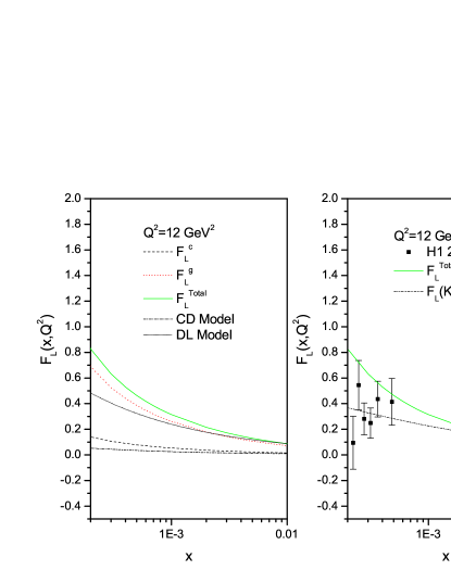
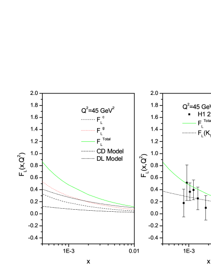
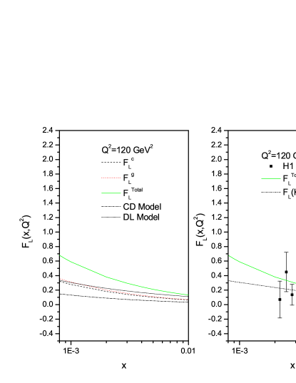
In Figs.1-3, we present the small $x$ behavior of the $F_{L}$ structure function according to the evolution equation (28) as a function of $x$ for $Q^{2}=12$, $45$ and $120~{}GeV^{2}$. In the left hand of these figures, we present the heavy contribution $F_{L}^{c}$, gluonic contribution $F_{L}^{g}$ and total $F_{L}^{Total}$ (heavy + gluonic) of longitudinal structure function with results of DL [30-33,62] and CD models [63]. In the right hand side, $F_{L}^{Total}$ has been presented with H1 data [54] with total error and on-shell limit of the $k_{T}$ factorization [64], where the transverse momentum of the gluon $k^{2}$ is much smaller than the virtuality of the photon ( $k^{2}{<<}Q^{2}$) and this is consistent with the collinear factorization as the $k_{T}$ factorization formula can be determined from the inclusive cross section in dipole representation. In all the cases longitudinal structure function $F_{L}$ increases towards smaller $x$ for a fixed $Q^{2}$. We compared our $F_{L}^{g}$ results with the results of DL model and $F_{L}^{c}$ results with the results of CD model. We observed that our $F_{L}^{c}$ results are somewhat higher than those of CD model in all $Q^{2}$. But though our $F_{L}^{g}$ results are somewhat higher than those of DL model, their differences decreases when $Q^{2}$ increase and they almost coincide at $120GeV^{2}$. On the otherhand, we observed that H1 data have been well described by our results as well as the results of $k_{T}$ factorization. Of course our results are slightly above than those of $k_{T}$ factorization. When $Q^{2}$ increases, our results become in better agreement with the data.
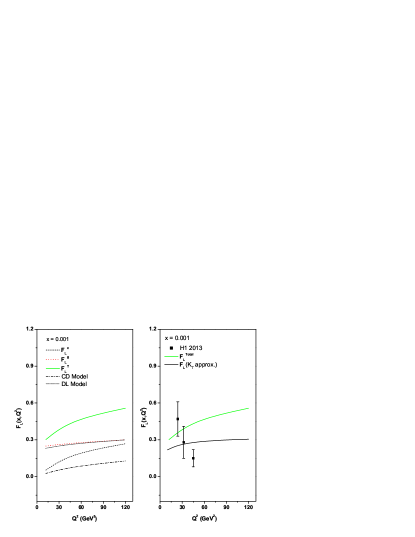
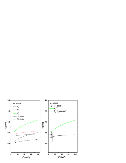
In Figs. 4-5, we present the same results of $F_{L}$ structure function as a function of $Q^{2}$ for small-$x$ values $x=0.001$ and $x=0.0004$. In all the cases longitudinal structure function $F_{L}$ increases towards higher $Q^{2}$ for a fixed $x$ and smaller $x$ for a fixed $Q^{2}$. Our $F_{L}^{g}$ results are very close to DL results especially at $x=0.001$. But our $F_{L}^{c}$ results are slightly higher than those of CD results. Also it is observed that the rate of increment of heavy longitudinal structure function $F_{L}^{c}$ is more than that of gluonic longitudinal structure function $F_{L}^{g}$, and both approach to closer values towards higher $Q^{2}$ values. Again comparing the $Q^{2}$-evolutions of total (heavy + gluonic) longitudinal structure function $F_{L}^{Total}$ with the results of $k_{T}$ factorization, it is seen that our results are comparable to H1 results, especially at higher-$x$, $x=0.001$; but somewhat higher in smaller-$x$, $x=0.0004$ in higher $Q^{2}$. On the other hand, $k_{T}$ factorization results are better in all the cases.
In our calculations, we use the DL model of the gluon distribution and also we set the running coupling constant according to the Table 1. For heavy contribution to the longitudinal structure function, we choose $m_{c}=1.3~{}GeV$ and the renormalization scale is $<\mu^{2}>=4m^{2}_{c}+Q^{2}/2$.

.4 IV. Conclusions

In conclusion, we have observed that the hard-pomeron behaviour for the longitudinal structure function dynamical behaviour gives the heavy quark effects to the light flavours at small-$x$. We can see in all figures the increase of our results for longitudinal structure function $F_{L}(x,Q^{2})$ towards smaller $x$ and higher $Q^{2}$ which is consistent with QCD calculations, reflecting the rise of gluon and charm (heavy) distribution inside proton in this region. Our results for gluonic and charm (heavy) longitudinal structure function do not exactly tally with results of DL and CD models respectively, as formers are somewhat higher than laters. Though $F_{L}^{g}$ is more or less comparable with results of DL models, $F_{L}^{c}$ is somewhat higher than that of CD models results. Our total results $F_{L}^{Total}$ and those of $k_{T}$ factorization are well within the data range. Lastly, one important conclusion is that charm (heavy) contribution to total longitudinal structure function is considerable one and can not be neglected especially at smaller $x$ and higher $Q^{2}$ region.

.5 Appendix A

The explicit forms of the first-, second- and third-order splitting functions are respectively [49-52]

$$P^{\rm LO}_{gg}(z) = 2C_{A}(\frac{z}{(1-z)_{+}}+\frac{(1-z)}{z}+z(1-z))$$ (33)

$$+\delta(1-z)\frac{(11C_{A}-4N_{f}T_{R})}{6},$$

where the ${}^{,}\text{plus}^{,}$ distribution is defined by

$$\int_{0}^{1}dz\frac{f(z)}{(1-z)_{+}}=\int_{0}^{1}dz\frac{f(z)-f(1)}{1-z},$$

$$P_{gg}^{\rm NLO} = C_{F}T_{F}(-16+8z+\frac{20}{3}z^{2}+\frac{4}{3z}$$

$$-(6+10z)\ln z-(2+2z)\ln^{2}z)$$

$$+C_{A}T_{F}(2-2z+\frac{26}{9}(z^{2}-z^{-1})$$

$$-\frac{4}{3}(1+z)\ln z-\frac{20}{9}P_{gg}(z))$$

$$+C_{A}^{2}(\frac{27}{2}(1-z)+\frac{67}{9}(z^{2}-z^{-1})$$

$$-(\frac{25}{3}-\frac{11}{3}z+\frac{44}{3}z^{2})\ln z$$

$$+4(1+z)\ln^{2}z+2P_{gg}(-z)S_{2}(z)$$

$$+(\frac{67}{9}-4\ln z\ln(1-z)$$

$$+\ln^{2}z-\frac{\pi^{2}}{3})P_{gg}(z)),$$

where

$$P_{gg}(z)=\frac{1}{(1-z)_{+}}+\frac{1}{z}-2+z(1-z),$$

and the function $S_{2}(z)=\int_{\frac{z}{1+z}}^{\frac{1}{1+z}}\frac{dy}{y}{\ln}(\frac{1-y}{y})$ is defined in terms of the dilogarithm function as

$$S_{2}(z)=-2Li_{2}(-z)+\frac{1}{2}\ln^{2}z-2\ln z\ln(1+z)-\frac{\pi^{2}}{6},$$

and

$$P_{gg}^{\rm NNLO} = 2643.521D0+4425.894\delta(1-z)$$ (35)

$$+3589L1-20852+3968z-3363z^{2}$$

$$+4848z^{3}+L0L1(7305+8757L0)$$

$$+274.4L0-7471L0^{2}+72L0^{3}-144L0^{4}$$

$$+14214z^{-1}+2675.8z^{-1}L0$$

$$+N_{f}(-412.172D0-528.723\delta(1-z)$$

$$-320L1-350.2+755.7z-713.8z^{2}$$

$$+559.3z^{3}+L0L1(26.15-808.7L0)$$

$$+1541L0+491.3L0^{2}+\frac{832}{9}L0^{3}$$

$$+\frac{512}{27}L0^{4}+182.96z^{-1}$$

$$+157.27z^{-1}L0)+N_{f}^{2}(-\frac{16}{9}D0$$

$$+6.4630\delta(1-z)-13.878+153.4z$$

$$-187.7z^{2}+52.75z^{3}$$

$$-L0L1(115.6-85.25z+63.23L0)$$

$$-3.422L0+9.680L0^{2}-\frac{32}{27}L0^{3}$$

$$-\frac{680}{243}z^{-1}),$$

where $L0=\ln z,~{}~{}L1=\ln(1-z)$ and $D0=\frac{1}{(1-z)_{+}}$.

.6 Appendix B

The $C^{c}_{L,g}$ is the charm coefficient longitudinal function in LO and NLO analysis and it is given by

$$C_{L,g}(z,\zeta) {\rightarrow} C^{(0)}_{L,g}(z,\zeta)+a_{s}(\mu^{2})[C_{L,g}^{(1)}(z,\zeta)$$

$$+\overline{C}_{L,g}^{(1)}(z,\zeta)ln\frac{\mu^{2}}{m_{c}^{2}}].$$

In LO analysis, this coefficient can be found in Refs.[15-16], as

$$C^{(0)}_{g,L}(z,\zeta)=-4z^{2}{\zeta}ln\frac{1+\beta}{1-\beta}+2{\beta}z(1-z),$$ (37)

where $\beta^{2}=1-\frac{4z\zeta}{1-z}$ and $\mu$ is the mass factorization scale, which has been put equal to the renormalization scales $\mu^{2}=4m_{c}^{2}$ or $\mu^{2}=4m_{c}^{2}+Q^{2}$, and in the NLO analysis we can use the compact form of these coefficients according to the Refs.[17-21].

Table 1: The QCD coupling and corresponding $\Lambda$ parameter for $N_{f}=4$, for LO, NLO and NNLO fits according to Refs.[65-67].

	$\alpha_{s}(M_{Z}^{2})$	$\Lambda_{QCD}(MeV)$
LO	0.130	220
NLO	0.119	323
NNLO	0.1155	235

References
1. A. Gonzalez-Arroyo, C. Lopez, and F.J. Yndurain, Phys. Lett. B98- 218(1981).
2. A. M. Cooper-Sarkar, G. Inglman, K. R. Long, R. G. Roberts, and D. H. Saxon , Z. Phys. C39- 281(1988).
3. R. G. Roberts, The structure of the proton, (Cambridge University Press 1990)Cambridge.
4. Aaron, F. D., et al., (H1 Collaboration), Phys. Lett. B665- 139(2008).
5. A. D. Martin, W. J. Stirling, R. S. Thorne, G. Watt, Eur. Phys. J. C70- 51(2010).
6. S. Moch and A.Vogt, JHEP0904- 218(1981).
7. R. S. Thorne, Phys. Lett.B418- 371(1998).
8. R. S. Thorne, arXiv:hep-ph/0511351 (2005).
9. A. D. Martin, W. J. Stirling, R. S.Thorne, Phys. Lett. B 635- 305(2006).
10. A. D. Martin, W. J. Stirling, R. S.Thorne, Phys. Lett. B636- 259(2006).
11. S. Moch, J. Vermaseren and A. Vogt, Nucl. Phys. B688- 101(2004).
12. S. Moch, J. Vermaseren and A. Vogt, Nucl. Phys. B691- 129(2004).
13. Moch, J. Vermaseren and A. Vogt, Phys. Lett. B606- 123(2005).
14. M. Gluck, C. Pisano and E. Reya, Phys. Rev. D77- 074002 (2008).
15. M. Gluk, E. Reya and A. Vogt, Z. Phys. C67- 433(1995).
16. M. Gluk, E. Reya and A. Vogt, Eur. Phys. J. C5- 461(1998).
17. E. Laenen, S. Riemersma, J. Smith and W. L. van Neerven, Nucl. Phys. B392- 162(1993).
18. A. Y. Illarionov, B. A. Kniehl and A. V. Kotikov, Phys. Lett.B663- 66(2008).
19. S. Catani, M. Ciafaloni and F. Hautmann, Preprint CERN-Th.6398/92, in Proceeding of the Workshop on Physics at HERA (Hamburg)2-690(1991).
20. S. Catani and F. Hautmann, Nucl. Phys. B427- 475(1994).
21. S. Riemersma, J. Smith and W. L. van Neerven, Phys. Lett. B347- 143(1995).
22. E. A. Kuraev, L. N. Lipatov and V. S. Fadin, Sov.Phys.JETP44- 443(1976).
23. E. A. Kuraev, L. N. Lipatov and V. S. Fadin, Sov. Phys. JETP45- 199(1977).
24. Y. Y. Balitsky and L. N. Lipatov, Sov. Journ. Nucl. Phys.28- 822(1978).
25. L.V.Gribov, E.M.Levin and M.G.Ryskin, Phys.Rep.100- 1(1983).
26. J. Kwiecinski, arXiv:hep-ph/9607221 (1996).
27. J. Kwiecinski, A.D.Martin and P.J.Sutton, Phys.Rev.D44- 2640(1991).
28. K.Kutak and A.M.Stasto, Eur.Phys.J.C41- 343(2005).
29. S.Bondarenko, arXiv:hep-ph/0808.3175(2008).
30. A. Donnachie and P. V. Landshoff, Phys. Lett. B296- 257(1992).
31. A. Donnachie and P. V. Landshoff, Phys. Lett. B437- 408(1998 ).
32. A. Donnachie and P. V. Landshoff, Phys. Lett. B550- 160(2002 ).
33. P.V.Landshoff, arXiv:hep-ph/0203084(2002).
34. P. Desgrolard, M. Giffon, E. Martynov and E. Predazzi, Eur. Phys. J. C18- 555(2001).
35. P. Desgrolard, M. Giffon and E. Martynov, Eur. Phys. J. C7- 655(1999).
36. A.A.Godizov, Nucl.Phys.A927 36(2014).
37. Yu. L. Dokshitzer, Sov. Phys. JETP6- 641(1977 ).
38. G. Altarelli and G. Parisi, Nucl. Phys. B126- 298(1997 ).
39. V. N. Gribov and L. N. Lipatov, Sov. J. Nucl. Phys.28- 822(1978).
40. M. B. Gay Ducati and V. P. B. Goncalves, Phys. Lett. B390- 401(1997).
41. K. Pretz, Phys.Lett.B311- 286(1993).
42. K. Pretz, Phys. Lett. B332- 393(1994).
43. A. V. Kotikov, arXiv:hep-ph/9507320(1995).
44. G. R. Boroun, JETP, Vol. 106,4- 701(2008).
45. G. R. Boroun and B. Rezaei, Eur. Phys. J. C72- 2221(2012).
46. G. R. Boroun and B. Rezaei, Eur. Phys. J. C73- 2412(2013).
47. M. Devee, R Baishya and J. K. Sarma, Eur. Phys.J. C72- 2036(2012).
48. R. Baishya, U. Jamil and J. K. Sarma, Phys. Rev. D79- 034030(2009).
49. S. Moch and A. Vogt, JHEP0904- 081(2009).
50. R. K. Ellis , W. J. Stirling and B. R. Webber, QCD and Collider Physics(Cambridge University Press)(1996).
51. C. Pisano, arXiv:hep-ph/0810.2215 (2008).
52. A. Retey, J. Vermaseren , Nucl. Phys. B604- 281(2001).
53. B. Lampe, E. Reya, Phys. Rep.332- 1(2000).
54. V. Andreev et al. [H1 Collaboration], Accepted by Eur. Phys. J. C, arXiv:hep-ex/1312.4821 (2013).
55. N. Ya. Ivanov, Nucl. Phys. B814- 142(2009).
56. N. Ya. Ivanov, Eur. Phys. J. C59- 647(2009).
57. I. P. Ivanov and N. Nikolaev, Phys. Rev. D65- 054004(2002).
58. G. R. Boroun and B. Rezaei, Nucl. Phys. B857-143(2012).
59. G. R. Boroun and B. Rezaei, Eur. Phys. Lett100- 41001(2012).
60. G. R. Boroun and B. Rezaei, Nucl. Phys. A929- 119(2014).
61. G.R.Boroun, Nucl. Phys. B884- 684(2014).
62. R. D. Ball and P. V. landshoff, J. Phys. G26- 672(2000).
63. N. N. Nikolaev and V. R. Zoller, Phys. Lett. B509- 283(2001).
64. K. Golec-Biernat and A. M. Stasto, Phys. Rev. D80 014006(2009).
65. A. D. Martin, R. G. Roberts, W. J. Stirling, R. S. Thorne, Phys. Lett. B531- 216(2002).
66. A. D. Martin, R. G. Roberts, W. J. Stirling, R. S. Thorne, Eur. Phys. J. C23- 73(2002).
67. A. D. Martin, R. G. Roberts, W. J. Stirling, R. S. Thorne, Phys. Lett. B604- 61(2004).

Figure 1: left: Dynamical light and heavy contributions to the total $F_{L}$ small $x$ for $Q^{2}=12~{}GeV^{2}$ at NNLO analysis, compared with DL [30-33,62] and CD [63] models respectively.
right: The total $F_{L}$ compared with $k_{T}$ factorization [64] and H1 data [54] with total error.

Figure 2: As in Fig. 1 but for $Q^{2}=45~{}GeV^{2}$.

Figure 3: As in Fig. 1 but for $Q^{2}=120~{}GeV^{2}$.

Figure 4: left: Dynamical light and heavy contributions to the total $F_{L}$ small $x$ for $x=0.001$ at NNLO analysis, compared with DL [30-33,62] and CD [63] models respectively.
right: The total $F_{L}$ compared with $k_{T}$ factorization [64] and H1 data [54] with total error.

Figure 5: As in Fig. 4 but for $x=0.0004$.