When Does Linear Stability Not Exclude Nonlinear Instability ?

Abstract

We describe a mechanism that results in the nonlinear instability of stationary states even in the case where the stationary states are linearly stable. This instability is due to the nonlinearity-induced coupling of the linearization’s internal modes of negative energy with the wave continuum. In a broad class of nonlinear Schrödinger (NLS) equations considered, the presence of such internal modes guarantees the nonlinear instability of the stationary states in the evolution dynamics. To corroborate this idea, we explore three prototypical case examples: (a) an anti-symmetric soliton in a double-well potential, (b) a twisted localized mode in a one-dimensional lattice with cubic nonlinearity, and (c) a discrete vortex in a two-dimensional saturable lattice. In all cases, we observe a weak nonlinear instability, despite the linear stability of the respective states.

Introduction. Among dispersive nonlinear partial differential equations, the nonlinear Schrödinger (NLS) model ablowitz1 ; sulem stands out as a prototypical system that has proved to be essential in modeling and understanding features of numerous areas in nonlinear physics. The relevant fields of application vary from optics and the propagation of the electric field envelope in optical fibers hasegawa ; kivshar , to the self-focusing and collapse of Langmuir waves in plasma physics zakh1 ; zakh2 . It is also encountered in the modeling of deep water and freak/rogue waves in the ocean benjamin ; onofrio , as well as in atomic physics and the dynamics of superfluids and atomic Bose-Einstein condensates becbook1 ; becbook2 ; rcg:BEC_BOOK .

One of the most customary ways to approach the experimental observations of nonlinear dispersive waves in these different physical systems is to explore the standing wave solutions that NLS models may possess and to understand their spectral and dynamical stability characteristics toddkeith . This is accomplished not only in homogeneous continuous media, but also in inhomogeneous and discrete ones, not only in one but also in higher dimensions jyang ; pelinov ; dnlsbook . Then, the conventional wisdom suggests that should the solution in the NLS model be found to be linearly (spectrally) stable, then it should be expected to be dynamically stable as well and hence a suitable candidate for observations in physical experiments. By linear stability here, we imply the absence of eigenvalues with nonzero real parts, as well as the absence of multiple and embedded imaginary eigenvalues with the exception of the zero eigenvalue generated by the symmetries of the NLS models.

In the present work, we explore an important, as well as generic nonlinear mechanism of instability of standing wave solutions, which are linearly stable. The instability is induced by the linearization’s internal modes of negative energy or negative Krein signature kapkev that correspond to simple imaginary eigenvalues and represent negative “directions” of the NLS energy at the standing wave solutions. While perfectly innocuous in the linear setting, these internal modes of negative energy can be in resonance with the wave spectrum or other internal modes due to nonlinearity, in which case they lead to the nonlinear instability of the standing wave solutions.

For a ground state, small amplitude excitations of the standing wave always increase the NLS energy so that the standing wave is an energetically stable minimum of the system, which is also dynamically stable. Internal modes for such ground states may only have positive energy or positive Krein signature kiv1 ; kiv2 . However, for many excited states, small amplitude excitations may decrease the NLS energy and still do not result in the appearance of linear instability. This has led to the widespread belief that energetic instability does not generically imply dynamical instability; instead “the energetic instability can only destabilize the system in the presence of dissipative terms which drive it towards configurations of lower energy” (p. 58 in becbook1 ). Our aim herein is to challenge this conventional wisdom and to establish through a diverse array of case examples that, in fact, generically, excited states bearing an energetic instability, will also manifest a dynamical one.

The initial mathematical formulation of the nonlinear mechanism of instability of excited states was obtained by Cuccagna scipio ; scipio1 , but these results have not been confirmed in physics literature by numerical or experimental evidence. In the present work, we give convincing numerical evidence of the nonlinear instability due to the internal modes of negative energy based on three case examples involving continuous and discrete NLS in one and two dimensions. The discovery of this nonlinear mechanism may broadly impact researchers in nonlinear physics enabling them to identify and to explain weak (nonlinear) instabilities of the standing waves observed in numerous experimental setups in atomic, optical, fluid or plasma systems related to this general framework.

Theoretical Formulation. The cubic NLS model in a generalized form reads:

$$i\partial_{t}u=-\nabla^{2}u+V(x)u+g|u|^{2}u,$$ (1)

where $u$ is a complex field, $V$ characterizes the external potential with a fast decay to zero at infinity, and $g$ is a coefficient that characterizes the self-focusing ($g<0$) or self-defocusing ($g>0$) nature of the nonlinearity. The standing wave solution takes the form $u(x,t)=e^{-i\omega t}\phi(x)$, where $\omega$ and $\phi$ are real.

The prototypical example of the nonlinear instability in the NLS model (1) occurs when the Schrödinger operator $-\nabla^{2}+V$ admits two simple negative eigenvalues (energy levels) $E_{0}<E_{1}$ such that

$$\frac{1}{2}|E_{1}|<|E_{1}-E_{0}|<|E_{1}|.$$ (2)

The ground state bifurcates for $\omega$ near $E_{0}$, whereas the excited state bifurcates for $\omega$ near $E_{1}$. In particular, the excited state can be represented by $\phi(x)=\epsilon u_{1}(x)+\mathcal{O}(\epsilon^{3})$, where $u_{1}$ is the $L^{2}$-normalized eigenfunction of $-\nabla^{2}+V$ for eigenvalue $E_{1}$, and $\epsilon$ is found from $\omega$ by

$$\omega=E_{1}+g\left(\int_{\mathbb{R}}|u_{1}|^{4}dx\right)\epsilon^{2}.$$

When considering the stability of the standing wave, we utilize the linearization, e.g. by means of

$$u(x,t)=e^{-i\omega t}\left[\phi(x)+\delta\left(a(x)e^{\lambda t}+\bar{b}(x)e^{\bar{\lambda}t}\right)\right],$$ (3)

with small parameter $\delta$ (independently of $\epsilon$), and obtain the spectral problem

$$H\psi=i\lambda\sigma_{3}\psi,$$ (4)

where $\psi=(a,b)^{T}$, $\sigma_{3}={\rm diag}(1,-1)$, and $H$ is given by

$$H=\left[\begin{array}[]{cc}-\Delta+V-\omega+2g\phi^{2}&g\phi^{2}\\ g\phi^{2}&-\Delta+V-\omega+2g\phi^{2}\end{array}\right].$$

If $\epsilon$ is small, it is easy to confirm that the spectral problem (4) has a double zero eigenvalue due to the gauge symmetry of the NLS model, the phonon band for $\lambda\in i(-\infty,-|\omega|]$ and $\lambda\in i[|\omega|,\infty)$, and a pair of internal modes at $\lambda=\pm i\Omega$ with $\Omega=E_{1}-E_{0}+\mathcal{O}(\epsilon^{2})>0$. With the condition (2), we note that $\Omega<|\omega|$ but $2\Omega>|\omega|$, hence the internal mode eigenfrequency is isolated from the phonon band but the second harmonic is embedded into the phonon band. The second harmonic can be generated by the nonlinear terms beyond the linear approximation (3). Also note that the mode energy is defined by

$$K=\langle H\psi_{\Omega},\psi_{\Omega}\rangle=-\Omega\int_{\mathbb{R}}(|a_{\Omega}|^{2}-|b_{\Omega}|^{2})dx,$$ (5)

where $\psi_{\Omega}=(a_{\Omega},b_{\Omega})^{T}$ is the eigenvector for the eigenvalue $\lambda=i\Omega$. Since $\Omega>0$ and $\psi_{\Omega}=(u_{0},0)^{T}+\mathcal{O}(\epsilon^{2})$, where $u_{0}$ is the $L^{2}$-normalized eigenfunction of $-\nabla^{2}+V$ for eigenvalue $\lambda_{0}$, then it follows that the internal mode has negative energy, that is, $K<0$.

Now we will explain why the internal mode of negative energy, when coupled with the phonon band due to the second harmonic, leads to the nonlinear instability of the standing wave. We shall consider the expansion in amplitudes of the internal mode

$$u(x,t)=e^{-i\omega t}\left[\phi(x)+\delta u_{1}(x,t)+\delta^{2}u_{2}(x,t)+\mathcal{O}(\delta^{3})\right],$$

with

$$u_{1}(x,t)=c(\tau)a_{\Omega}(x)e^{i\Omega t}+\bar{c}(\tau)\bar{b}_{\Omega}(x)e^{-i\Omega t},$$

where $c(\tau)$ is the complex amplitude of the internal mode evolving in slow time $\tau=\delta^{2}t$. Note that because $H+\Omega\sigma_{3}$ is a self-adjoint operator, we can choose the internal mode $(a_{\Omega},b_{\Omega})^{T}$ to be real. Using the expansion above, similar to what was done in the case of internal modes of positive energy kiv2 , we obtain the explicit representation of the second-order correction term

$$u_{2}(x,t)=c^{2}a_{2}(x)e^{2i\Omega t}+|c|^{2}a_{0}(x)+\bar{c}^{2}\bar{b}_{2}(x)e^{-2i\Omega t},$$

where $\psi_{2}=(a_{2},b_{2})^{T}$ and $\psi_{0}=(a_{0},a_{0})^{T}$ are obtained from suitable solutions of the inhomogeneous problems

$$(H+2\Omega\sigma_{3})\psi_{2}=-g\phi\left[\begin{array}[]{c}(a_{\Omega}+2b_{\Omega})a_{\Omega}\\ (2a_{\Omega}+b_{\Omega})b_{\Omega}\end{array}\right]$$ (8)

and

$$H\psi_{0}=-2g\phi(a_{\Omega}^{2}+a_{\Omega}b_{\Omega}+b_{\Omega}^{2})\left[\begin{array}[]{c}1\\ 1\end{array}\right].$$ (11)

Because $2\Omega>|\omega|$, the correction term $\psi_{2}$ is bounded but not decaying at infinity. We apply the Sommerfeld radiation condition

$$\psi_{2}(x)\to R_{\Omega}e_{2}e^{\mp ik_{\Omega}x}\quad\mbox{\rm as}\quad x\to\pm\infty,$$ (12)

where $e_{2}=(0,1)$, $k_{\Omega}=\sqrt{2\Omega-|\omega|}$, and the radiation tail amplitude $R_{\Omega}$ is a uniquely determined complex coefficient. Because of the Sommerfeld radiation condition (12), the second harmonic $(a_{2},b_{2})$ is given by complex functions.

Proceeding to the third-order correction term, as in kiv2 , we obtain the evolution equation for the amplitude $c(\tau)$ in slow time $\tau=\delta^{2}t$,

$$iK\frac{dc}{d\tau}+\Omega\beta|c|^{2}c=0,$$ (13)

where $K$ is given by (5) and $\beta$ is found from the projections as

$$\beta = 2g\int_{\mathbb{R}}\phi\left[a_{2}a_{\Omega}(a_{\Omega}+2b_{\Omega})+b_{2}b_{\Omega}(2a_{\Omega}+b_{\Omega})\right]dx$$

$$+4g\int_{\mathbb{R}}a_{0}(a_{\Omega}^{2}+a_{\Omega}b_{\Omega}+b_{\Omega}^{2})dx$$

$$+g\int_{\mathbb{R}}\left(a_{\Omega}^{4}+4a_{\Omega}^{2}b_{\Omega}^{2}+b_{\Omega}^{4}\right)dx.$$

Note that the coefficients in front of $(a_{2},b_{2})$ correspond to the source term of the inhomogeneous equations (8). The parameter $\beta$ is complex because the correction terms $(a_{2},b_{2})$ are complex. Using Eqs. (8) and (12), we obtain

$$2i{\rm Im}(\beta) = 2\left(\bar{a}_{2}^{\prime}a_{2}+\bar{b}_{2}^{\prime}b_{2}-\bar{a}_{2}a_{2}^{\prime}-\bar{b}_{2}b_{2}^{\prime}\right)\biggr{|}_{x\to-\infty}^{x\to+\infty}$$ (14)

$$= 8ik_{\Omega}|R_{\Omega}|^{2}.$$

Eq. (14) recovers the so-called Fermi golden rule with $k_{\Omega}|R_{\Omega}|^{2}>0$ for all generic cases with nonvanishing coefficient $R_{\Omega}$.

Introducing the square amplitude $Q(\tau)=|c(\tau)|^{2}$, we obtain a simple differential equation

$$K\frac{dQ}{d\tau}=-8\Omega k_{\Omega}|R_{\Omega}|^{2}Q^{2},$$ (15)

starting with the positive initial value $Q(0)$. For the internal mode of positive energy with $K>0$, this equation leads to the slow (i.e., power law) decay of the internal mode in time kiv2 . For the internal mode of negative energy $K<0$, this equation guarantees the power-law growth of the internal mode in time and eventual blow up of the quadratic approximation in (15), although this growth is typically saturated by the nonlinearity. Mathematical justification of the normal form equation (15) and the Fermi golden rule (14) can by found in scipio ; scipio1 .

Case Example 1: anti-symmetric soliton in double-well potentials. The dynamics of the anti-symmetric (so-called $\pi$) solitons in a double well potential has been explored extensively in the recent physical literature (see e.g. malomedbook ) motivated by experiments in atomic markus ; leblanc ; zibold and optical zhigang ; haelt physics. In comparison to the work presented herein, such solitons were realized experimentally for short dynamical time scales, for which no dynamical instability was detected zibold . Here we report on the weak (nonlinear) instability of the anti-symmetric solitons in the NLS model (1) with the repulsive interaction $g=-1$ and the double-well potential

$$V(x)=V_{0}\left({\rm sech}^{2}(x-x_{0})+{\rm sech}^{2}(x+x_{0})\right),$$ (16)

for which we take $V_{0}=-1$ and $x_{0}=2$. For $\omega=-0.4$, the frequency of the internal mode of the anti-symmetric soliton is $\Omega\approx 0.203$ (i.e., $\Omega<|\omega|$ but $2\Omega>|\omega|$) ensuring the second harmonic occurs inside the phonon band.

In Fig. 1, we monitor the dynamical evolution of the anti-symmetric soliton, perturbed by the internal mode. We observe the slow manifestation of a dynamical instability, both in the space-time evolution in the top panel, as well as more concretely in the time evolution of the maximal amplitudes in the two potential wells in the bottom panel. The longer term dynamics shows that the growing oscillatory dynamics of the internal mode does not saturate but returns to the initial state leading to recurrent dynamics.

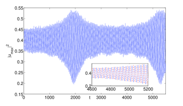
Figure 1: (Color Online) The top panel shows the space-time evolution of a perturbed anti-symmetric soliton in the NLS model (3) with the double-well potential (16). The slow growth over time is further illustrated in the bottom panel of the figure containing the evolution of the maximal amplitude in the left and right potential wells by solid (blue) and dashed (red) line. Inset: detail of the growth dynamics.

Case Example 2: the twisted localized mode in a one-dimensional lattice with cubic nonlinearity. We examine a twisted localized mode in the one-dimensional cubic NLS lattice dnlsbook . Such “dipolar” states have been previously explored in both 1d kip1d and 2d zhig2d optical experiments. The discrete NLS equation is a prototypical model of optical waveguide arrays in nonlinear optics motireview . We take the discrete NLS equation in the standard form:

$$i\dot{u}_{n}=-C\Delta_{2}u_{n}-|u_{n}|^{2}u_{n}.$$ (17)

Here $u_{n}$ plays the role of the envelope of the electric field at the $n$-th waveguide and $C$ represents the strength of the evanescent coupling between the waveguides, while $\Delta_{2}$ stands for the standard 3-point stencil in the one-dimensional lattice.

The twisted localized modes can be exactly represented in the limit of $C=0$ (so-called anti-continuum limit) as $u_{n}(t)=e^{it}(\delta_{n,0}-\delta_{n,1})$, setting $\omega=-1$ without loss of generality. As $C\neq 0$ increases, as shown in pelikev1 , the solution is linearly stable but it has one internal mode of negative energy with the frequency $\Omega=\mathcal{O}(C^{1/2})$ as $C\to 0$. For small $C$, this frequency is isolated from the phonon band, which corresponds to the frequencies in the interval $[1,1+4C]$. For $C=0.01$, the internal mode frequency is $\Omega\approx 0.204$ so that the condition $2\Omega>|\omega|$ is not satisfied. While this case is unstable too via the proposed mechanism, the instability only arises through a higher harmonic (the fifth harmonic, in fact) of the mode frequency. That is why the instability is not visible on the time scale of our dynamical simulations shown in the top panel of Fig. 2.

On the other hand, for the case of $C=0.07$, the internal mode frequency is $\Omega\approx 0.598$ and $2\Omega>|\omega|$ is satisfied. In the dynamics of the bottom panel of Fig. 2, we thus initialize with such a solution, perturbed by this internal mode. We can clearly see in this panel (showing the evolution of one of the two central amplitudes at $n_{0}=0$) that there is very slow growth reminiscent of a power law. After this instability manifests itself, it eventually saturates. The theory does not reveal any information about the ultimate fate of the dynamics. The numerics suggest a resulting genuinely periodic state for the modulus, hence a genuinely quasi-periodic (or breather-on-breather kw ) state for the system. This, in turn, suggests that it would be quite worthwhile to further explore such states dynamically.

Figure 2: (Color Online) Evolution of twisted localized modes in the discrete NLS model (17). Top: time evolution of the 4 center-most sites (i.e., the two central ones and their immediate neighbors) of the structure for $C=0.01$; no instability is manifested. The insets show a zoom-in of the relevant sites revealing their oscillatory behavior. Bottom: the evolution of one of the central sites for $C=0.07$ (the inset shows its envelope illustrating the unstable evolution). In both panels $n_{0}=0$.

Case Example 3: a discrete vortex in a two-dimensional saturable lattice. Our third example is also highly motivated physically: we inspect discrete vortices in two-dimensional lattices that were robust enough dynamically to also be accessible in the optical observations within photorefractive optical crystals  neshev2 ; moti2 . Here, to comply with the photorefractive nature of the nonlinearity and to illustrate the genericity of our results a saturable nonlinearity has been implemented jiankenjp (although the results would still hold in the cubic case). The discrete saturable NLS equation takes the form

$$i\dot{u}_{n,m}=-C\Delta_{2}u_{n,m}+\frac{u_{n,m}}{1+|u_{n,m}|^{2}},$$ (18)

where $\Delta_{2}$ in this case stands for the standard 5-point stencil in the two-dimensional square lattice.

Our example shown in Fig. 3 corresponds to the case of $C=0.09$. In this case, the phonon band corresponds to the frequencies in the interval $[1-\omega,1-\omega+8C]$. The discrete vortex consisting of four excited principal sites at the center of the chain with phases of approximately $0$, $\pi/2$, $\pi$ and $3\pi/2$ is found for $\omega=0.65$ to possess three internal modes with eigenvalues $\Omega=0.012$, $\Omega=0.167$ and $\Omega=0.191$. Among the three, and while the structure is linearly stable, the last one has its second harmonic lying within the phonon band, hence we anticipate its destabilization by the mechanism reported herein. Indeed, this is what we observe in Fig. 3. However, the instability in this case appears to be far more “detrimental” for the state in comparison to the previous examples. In particular, the slow growth of the instability eventually gives rise to a dramatic event through which one among the four vortex principal nodes picks up most of the power in the system, while the other three considerably decrease in power. The resulting dynamics effectively leads to a single-site ground state configuration of the two-dimensional lattice.

Figure 3: (Color Online) The top panel shows the modulus time evolution of $|u_{n=0,m=0,\pm 1}|$, while the bottom panel illustrates the corresponding evolution of $|u_{n=1,m=0,\pm 1}|$ [i.e., 4 sites constituting the discrete vortex ($(0,0)$, $(0,1)$, $(1,0)$ and $(1,1)$) and two immediately adjacent ones ($(0,-1)$ and $(1,-1)$)]. Among the 4 central sites, only one (dashed red in the top panel) grows in power, while the other 3 (solid blue in the top and bottom and dashed red in the bottom) decrease in amplitude. The neighboring sites also remain at low amplitudes (green dash-dotted).

Conclusions. In the present work, we examined a previously unexplored mechanism for nonlinear instability which is generic for excited states of nonlinear Schrödinger systems. The generality and potential experimental ramifications (through numerical experiments herein) of our findings were also discussed. It was shown that the mechanism occurs independently of the discrete or continuum, one- or multi-dimensional, cubic or saturable nature of the underlying NLS models, as long as the excited nature of the state is manifested via the internal modes of negative energy. These are found to give rise to a weak (power law in its apparent manifestation) instability that eventually deforms, or in some cases (e.g., the discrete vortex) completely destroys the configuration.

While the mechanism presented herein is explicitly established, there are numerous questions that are worthy of further investigation, in addition to its potential experimental demonstration. It would be relevant to confirm that the mechanism can be numerically observed also in the case of higher order harmonics e.g., when $n\Omega<|\omega|$ but $(n+1)\Omega>|\omega|$. Additionally, it would be relevant to explore whether the mechanism is applicable to other dispersive wave systems of intense current interest, such as, e.g., nonlinear Dirac equations.

References

- (1) M.J. Ablowitz, B. Prinari and A.D. Trubatch, Discrete and Continuous Nonlinear Schrödinger Systems, Cambridge University Press (Cambridge, 2004).
- (2) C. Sulem and P.L. Sulem, The Nonlinear Schrödinger Equation, Springer-Verlag (New York, 1999).
- (3) A. Hasegawa, Solitons in Optical Communications, Clarendon Press (Oxford, NY 1995).
- (4) Yu.S. Kivshar and G.P. Agrawal, Optical solitons: from fibers to photonic crystals, Academic Press (San Diego, 2003).
- (5) V.E. Zakharov, Collapse and Self-focusing of Langmuir Waves, Handbook of Plasma Physics, (M.N. Rosenbluth and R.Z. Sagdeev eds.), vol. 2 (A.A. Galeev and R.N. Sudan eds.), 81–121, Elsevier (1984).
- (6) V.E. Zakharov, Collapse of Langmuir waves, Sov. Phys. JETP 35 (1972) 908–914.
- (7) T.B. Benjamin and J.E. Feir, J. Fluid Mech. 27, 417 (1967).
- (8) M. Onorato, A.R. Osborne, M. Serio, and S. Bertone, Phys. Rev. Lett. 86, 5831 (2001).
- (9) L.P. Pitaevskii and S. Stringari, Bose-Einstein Condensation, Oxford University Press (Oxford, 2003).
- (10) C.J. Pethick and H. Smith, Bose-Einstein condensation in dilute gases, Cambridge University Press (Cambridge, 2002).
- (11) P.G. Kevrekidis, D.J. Frantzeskakis, and R. Carretero-González Emergent Nonlinear Phenomena in Bose-Einstein Condensates: Theory and Experiment. Springer Series on Atomic, Optical, and Plasma Physics, Vol. 45 (Heidelberg, 2008).
- (12) T. Kapitula, and K. Promislow, Spectral and dynamical stability of nonlinear waves, Springer-Verlag (New York, 2013).
- (13) J. Yang, Nonlinear Waves in Integrable and Nonintegrable Systems. SIAM (Philadelphia, 2010).
- (14) D.E. Pelinovsky, Localization in Periodic Potentials, Cambridge University Press (Cambridge, 2011).
- (15) P.G. Kevrekidis, The Discrete Nonlinear Schrödinger Equation Springer-Verlag (Heidelberg, 2009).
- (16) T. Kapitula, P.G. Kevrekidis, and B. Sandstede, Phys. D 195 263 (2004).
- (17) Yu.S. Kivshar, D.E. Pelinovsky, T. Cretegny, and M. Peyrard, Phys. Rev. Lett. 80, 5032–5035 (1998)
- (18) D.E. Pelinovsky, Yu.S. Kivshar, and V.V. Afanasjev, Physica D 116, 121–142 (1998).
- (19) S. Cuccagna, Phys. D 238, 38 (2009).
- (20) S. Cuccagna, and M. Maeda, arXiv:1309.0655.
- (21) B.A. Malomed (Ed.), Spontaneous symmetry-breaking, self-trapping and Josephson oscillations, Springer-Verlag (Heidelberg, 2013).
- (22) M. Albiez, R. Gati, J. Fölling, S. Hunsmann, M. Cristiani, and M. K. Oberthaler, Phys. Rev. Lett. 95, 010402 (2005).
- (23) L. J. LeBlanc, A. B. Bardon, J. McKeever, M. H. T. Extavour, D. Jervis, J. H. Thywissen, F. Piazza, and A. Smerzi, Phys. Rev. Lett. 106, 025302 (2011).
- (24) T. Zibold, E. Nicklas, C. Gross, and M.K. Oberthaler, Phys. Rev. Lett. 105, 204101 (2010).
- (25) P.G. Kevrekidis, Z. Chen, B. A. Malomed, D. J. Frantzeskakis, and M. I. Weinstein, Phys. Lett. A 340, 275 (2005).
- (26) C. Cambournac, T. Sylvestre, H. Maillotte , B. Vanderlinden, P. Kockaert, Ph. Emplit, and M. Haelterman, Phys. Rev. Lett. 89, 083901 (2002).
- (27) M. Stepić, E. Smirnov, C. Rüter, L. Prönneke, D. Kip, and V. Shandarov, Phys. Rev. E 74, 046614 (2006).
- (28) J. Yang, A. Bezryadina, I. Makasyuk, and Z. Chen, Opt. Lett. 29, 1662 (2004).
- (29) F. Lederer, G.I. Stegeman, D.N. Christodoulides, G. Assanto, M. Segev, and Y. Silberberg, Phys. Rev. 463, 1 (2008).
- (30) D.E. Pelinovsky, P.G. Kevrekidis, and D.J. Frantzeskakis, Phys. D 212, 1 (2005).
- (31) P.G. Kevrekidis, and M.I. Weinstein, Math. Comp. Simul. 62, 65 (2003).
- (32) D.N.Neshev, T.J. Alexander, E.A. Ostrovskaya, Yu.S. Kivshar, H. Martin, I. Makasyuk, and Z. Chen, Phys. Rev. Lett. 92, 123903 (2004).
- (33) J.W. Fleischer, G. Bartal, O. Cohen, O. Manela, M. Segev, J. Hudock and D.N. Christodoulides, Phys. Rev. Lett. 92, 123904 (2004).
- (34) J. Yang, New J. Phys. 6, 47 (2004).