∎
Mostafa.HaghirChehreghani@cs.kuleuven.be, Maurice.Bruynooghe@cs.kuleuven.be
Mining Rooted Ordered Trees under Subtree Homeomorphism
Abstract
Mining frequent tree patterns has many applications in different areas such as XML data, bioinformatics and World Wide Web. The crucial step in frequent pattern mining is frequency counting, which involves a matching operator to find occurrences (instances) of a tree pattern in a given collection of trees. A widely used matching operator for tree-structured data is subtree homeomorphism, where an edge in the tree pattern is mapped onto an ancestor-descendant relationship in the given tree. Tree patterns that are frequent under subtree homeomorphism are usually called embedded patterns. In this paper, we present an efficient algorithm for subtree homeomorphism with application to frequent pattern mining. We propose a compact data-structure, called occ, which stores only information about the rightmost paths of occurrences and hence can encode and represent several occurrences of a tree pattern. We then define efficient join operations on the occ data-structure, which help us count occurrences of tree patterns according to occurrences of their proper subtrees. Based on the proposed subtree homeomorphism method, we develop an effective pattern mining algorithm, called TPMiner. We evaluate the efficiency of TPMiner on several real-world and synthetic datasets. Our extensive experiments confirm that TPMiner always outperforms well-known existing algorithms, and in several cases the improvement with respect to existing algorithms is significant.
Keywords:
XML data rooted ordered trees frequent tree patterns subtree homeomorphism embedded subtrees1 Introduction
Many semi-structured data such as XML documents are represented by rooted ordered trees. One of the most important problems in the data mining of these tree-structured data is frequent tree pattern discovery. Mining frequent tree patterns is very useful in various domains such as network routing 8 , bioinformatics 36 and user web log data analysis Ivancsy . Furthermore, it is a crucial step in several other data mining and machine learning problems such as clustering and classification 37 .
In general, algorithms proposed for finding frequent tree patterns include two main phases: 1) generating candidate tree patterns, and 2) counting the frequency of every generated tree pattern in a given collection of trees (called the database trees from now on). The generation step (which involves a refinement operator) is computationally easy. There are methods, such as rightmost path extension, that can generate efficiently all non-redundant rooted ordered trees, i.e., each in computational time 36 and 2 . The frequency counting step is computationally expensive. Empirical comparison of these two phases can be found e.g., in 4 , where Chi et. al. showed that a significant part of the time required for finding frequent patterns is spent on frequency counting. Thereby, the particular method used for frequency counting can significantly affect the efficiency of the tree mining algorithm.
The frequency counting step involves a matching operator 12 . A widely used matching operator between a tree pattern and a database tree is subtree homeomorphism; an injective mapping of the vertices such that an edge in the tree pattern is mapped onto an ancestor-descendant relationship in the database tree. Frequent tree patterns under subtree homeomorphism are called embedded patterns. They have many applications in different areas. Zaki et. al. 37 presented XRules, a classifier based on frequent embedded tree patterns, and showed its high performance compared to classifiers such as SVM. Ivancsy and Vajk used frequent embedded tree patterns for analyzing the navigational behavior of the web users Ivancsy .
Two widely used frequency notions are per-tree frequency, where only the occurrence of a tree pattern inside a database tree is important; and per-occurrence frequency, where the number of occurrences is important, too. While there exist algorithms optimized for the first notion 36 , 24 and 26 , this notion is covered also by the algorithms proposed for the second notion. Per-occurrence frequency counting is computationally more expensive than per-tree frequency counting. In the current paper, our concern is per-occurrence frequency. An extensive discussion about the applications in which the second notion is preferred can be found e.g., in 23 . One of the investigated examples is a digital library where author information are separately stored in database trees in some form, e.g., author–book–area–publisher. A user may be interested in finding out information about the popular publishers of every area. Then, the repetition of items within a database tree becomes important, hence, per-occurrence frequency is more suitable than per-tree frequency 23 .
Two categories of approaches have been used for counting occurrences of tree patterns under subtree homeomorphism. The first category includes approaches that use one of the algorithms proposed for subtree homeomorphism between two trees. HTreeMiner 36 employs such an approach. The second category includes approaches that store the information representing/encoding the occurrences of tree patterns. Then, when the tree pattern is extended to a larger one, its stored information is also extended, in a specific way, to represent the occurrences of the extended pattern. These approaches are sometimes called vertical approaches. VTreeMiner 36 and MB3Miner 23 are examples of the methods that use such vertical approaches. As studied in 36 , vertical approaches are more efficient than the approaches in the first category. Many efficient vertical algorithms are based on the numbering scheme proposed by Dietz Dietz . This scheme uses a tree traversal order to determine the ancestor-descendant relationship between pairs of vertices. It associates each vertex with a pair of numbers, sometimes called scope. For instance, VTreeMiner and TreeMinerD 36 and TwigList Qin use this scheme in different forms, to design efficient methods for counting occurrences of tree patterns.
The problem with these algorithms is that in order to count all occurrences, they use data-structures that represent whole occurrences. This renders the algorithms inefficient, especially when patterns are large and have many occurrences in the database trees. In the worst case, the number of occurrences of a tree pattern can be exponential in terms of the size of pattern and database Chisurvey . Therefore, keeping track of all occurrences can significantly reduce the efficiency of the algorithm, in particular when tree patterns have many occurrences in the database trees.
The main contribution of the current paper is to introduce a novel vertical algorithm for the class of rooted ordered trees. It uses a more compact data-structure, called occ (an abbreviation for occurrence compressor) for representing occurrences, and a more efficient subtree homeomorphism algorithm based on Dietz’s numbering scheme Dietz . An occ data-structure stores only information about rightmost paths of occurrences and hence can represent/encode all occurrences that have the rightmost path in common. The number of such occurrences can be exponential, even though the size of the occ is only , where is the length of the rightmost path of the tree pattern. We present efficient join operations on occ that help us to efficiently calculate the occurrence count of tree patterns from the occurrence count of their proper subtrees. Furthermore, we observed that in most of widely used real-world databases, while many vertices of a database tree have the same label, no two vertices on the same path are identically labeled. For this class of database trees, worst case space complexity of our algorithm is linear; a result comparable to the best existing results for per-tree frequency. We note that for such databases, worst case space complexity of the well-known existing algorithms for per-occurrence frequency, such as VTreeMiner 36 and MB3Miner 23 , is still exponential. Based on the proposed subtree homeomorphism method, we develop an efficient pattern mining algorithm, called TPMiner. To evaluate the efficiency of TPMiner, we perform extensive experiments on both real-world and synthetic datasets. Our results show that TPMiner always outperforms most efficient existing algorithms such as VTreeMiner 36 and MB3Miner 23 . Furthermore, there are several cases where the improvement of TPMiner with respect to existing algorithm is very significant.
In Section 2, preliminaries and definitions related to the tree pattern mining problem are introduced. In Section 3, a brief overview on related work is given. In Section 4, we present the occ data-structure and our subtree homeomorphism algorithm. In Section 5, we introduce the TPMiner algorithm for finding frequent embedded tree patterns from rooted ordered trees. We empirically evaluate the effectiveness of TPMiner in Section 6. Finally, the paper is concluded in Section 7.
2 Preliminaries
We assume the reader is familiar with the basic concepts in graph theory. The interested reader can refer to e.g., Diestel . An undirected (vertex-labeled) graph consists of a vertex set , an edge set , and a labeling function : which assigns a label from a finite set to every vertex in . is a directed graph if is: , where is the Cartesian product. We use the notations , and to refer to the set of vertices, the set of edges (or arcs) and the labeling function of , respectively. The size of is defined as the number of vertices of . Two graphs and (either both are directed or both are undirected) are identical, written as , if , , and . A path from a vertex to a vertex in a directed graph is a sequence of vertices such that , , . The length of a path is defined as its number of edges (number of vertices minus 1). A cycle is a path with .

An undirected graph not containing any cycles is called a forest and a connected forest is called a (free) tree. A rooted tree is a directed acyclic graph (DAG) in which: 1) there is a distinguished vertex, called root, that has no incoming edges, 2) every other vertex has exactly one incoming edge, and 3) there is an unique path from the root to any other vertex. In a rooted tree , is the parent of ( is the child of ) if . The transitive closure of the parent-child relation is called the ancestor-descendant relation. A rooted ordered tree is a rooted tree such that there is an order over the children of every vertex. Throughout this paper, we refer to rooted ordered trees simply as trees. Preorder traversal of a tree is defined recursively as follows: first, visit ; and then for every child of from left to right, perform a preorder traversal on the subtree rooted at . The position of a vertex in the list of visited vertices during a preorder traversal is called its preorder number. We use to refer to the preorder number of vertex . For instance, in Figure 1, numbers next to vertices of tree present their preorder numbers. The rightmost path of is the path from to the last vertex of visited in the preorder traversal. For example, in Figure 1, the vertices labeled by and form the rightmost path of . Two distinct vertices and are relatives if is neither an ancestor nor a descendant of . With , is a left relative of , otherwise, it is a right relative. For example, in tree of Figure 1, vertices and are relatives and vertex is a right relative of vertex .
A tree is a rightmost path extension of a tree iff there exist vertices and such that: (i) , (ii) , (iii) is on the rightmost path of , and (iv) in , is a right relative of all children of . We say that is the rightmost path extension of with attached at and we denote as . For instance, in Figure 1, is a rightmost path extension of , where the new vertex is labeled by , the existing vertex is also labeled by , and is added to as the rightmost child.
A tree is subtree homeomorphic to a tree (denoted by ) iff there is a mapping such that: (i) , (ii) : is the parent of in iff , and (iii) : . For example, in Figure 1, dashed lines present a subtree homeomorphism mapping from to . Under subtree isomorphism and homomorphism, the ancestor-descendant relationship between and in (ii) is strengthened into the parent-child relationship; under subtree homomorphism, (iii) is weakened into: , i.e., successive children of a vertex in the pattern can be mapped onto the same vertex in the database tree. is isomorphic to (denoted ) iff is subtree isomorphic to and .
Note that a pattern under a subtree morphism can have several mappings to the same database tree . When the matching operator is subtree homeomorphism, every mapping is called an occurrence (or embedding) of in . An occurrence (embedding) of a vertex is an occurrence (embedding) of the pattern consisting of the single vertex . The number of occurrences of in is denoted by .
Given a database consisting of trees and a tree , per-tree support (or per-tree frequency) of in is defined as: . Per-occurrence support (or per-occurrence frequency) of in is defined as: . In this paper, our focus is per-occurrence support. For the sake of simplicity, we use the term support (or frequency) instead of per-occurrence support (or per-occurrence frequency), and denote it by . is frequent ( is a frequent embedded pattern), iff its support is greater than or equal to a user defined integer threshold . The problem studied in this paper is as follows: given a database consisting of trees and an integer , find every frequent pattern such that .

We observe that when per-occurrence support is used, anti-monotonicity might be violated: it is possible that the support of is greater than or equal to , but it has a subtree whose support is less than . For example, consider the database tree of Figure 2 and suppose that is . Then, while the pattern is infrequent, it has two frequent supertrees and . Therefore, in a more precise (and practical) definition, which is also used by algorithms such as VTreeMiner 36 , tree is frequent iff: 1) , and 2) the subtree generated by removing the rightmost vertex of is frequent. This means only frequent trees are extended to generate larger patterns.
3 Related work
Recently, many algorithms have been proposed for finding frequent embedded patterns from a database of tree-structured data that work with both per-tree and per-occurrence frequencies. Zaki presented VTreeMiner 36 to find embedded patterns from trees. For frequency counting he used an efficient data structure, called scope-list, and proposed rightmost path extension to generate non-redundant candidates. Later, he proposed the SLEUTH algorithm to mine embedded patterns from rooted unordered trees 35 . Tan et. al. 23 introduced the MB3Miner algorithm, where they use a unique occurrence list representation of the tree structure, that enables efficient implementation of their Tree Model Guided (TMG) candidate generation. TMG can enumerate all the valid candidates that fit in the structural aspects of the database. Chaoji et. al. Chaoji introduced a generic pattern mining approach that supports various types of patterns and frequency notions. A drawback of these algorithms is that in order to count the number of occurrences of a tree pattern in a database tree , they need to keep track of all occurrences of in . For example, in VTreeMiner, for every occurrence of in a separate element is stored in scope-list, that consists of the following components: () which is the identifier of the database tree that contains the occurrence, () which is , and () which is the scope of , where is the rightmost vertex of . In the current paper, we propose a much more compact data-structure that can represent/encode all occurrences that have the rightmost path in common in space, where is the length of the rightmost path of . The number of such occurrences can be exponential. We then present efficient algorithms that calculate the occurrence count of tree patterns from the occurrence count of their proper subtrees.
There also exist several algorithms optimized for per-tree frequency. Zaki presented TreeMinerD 36 based on the SV-list data-structure. Tatikonda et. al. 24 developed TRIPS and TIDES using two sequential encodings of trees to systematically generate and evaluate tree patterns. Wang et. al. 26 proposed XSpanner that uses a pattern growth-based method to find embedded tree patterns. The literature contains also many algorithms for mining patterns under subtree isomorphism; examples are in 2 , 18 , Balcazar , Chehreghani1 and Chehreghani2 . From the applicability point of view, for instance in the prediction task, when longer range relationships are relevant, subtree homeomorphism becomes more useful than subtree isomorphism. For a more comprehensive study of related work, the interested reader can refer to e.g., Chisurvey .
A slightly different problem over rooted, ordered, and labeled trees is the tree inclusion problem: can a pattern be obtained from a tree by deleting vertices from . In our terminology, is present in under subtree homeomorphism? Bille and Gortz Bille recently proposed a novel algorithm that runs in linear space and subquadratic time, improving upon a series of polynomial time algorithms that started with the work in 12 .
4 Efficient tree mining under subtree homeomorphism
In this section, we present our method for subtree homeomorphism of rooted ordered trees. First in Section 4.1, we introduce the notion of occurrence tree and its rightmost path extension. Then in Section 4.2, we present the occ-list data-structure and, in Section 4.3, the operators for this data structure. In Section 4.4, we analyze space and time complexities of our proposed frequency counting method. We briefly compare our approach with other vertical frequency counting methods in Section 4.5.
4.1 Occurrence trees and their extensions
Under rightmost path extension, a pattern with vertices is generated from a pattern with vertices by adding a vertex , as the rightmost child, to a vertex in the rightmost path of . Occurrences of are rightmost path extensions of occurrences of with an occurrence of . Therefore, an interesting way to construct occurrences of is to look at the occurrences of that can be a rightmost path extension of an occurrence of . First, we introduce the notion of occurrence tree. Then, we present the conditions under which a rightmost path extension of an occurrence tree yields another occurrence tree.
Definition 1 (Occurrence tree)
Given an occurrence of in , we define the occurrence tree as follows: (i) , (ii) , for every , , and (iii) .

Notice, when and is not the parent of in , then all intermediate vertices on the path from to are not part of . For example, in Figure 3, the tree has occurrences in tree .
Selecting a vertex not yet in the occurrence tree and performing a rightmost path extension does not always result in another occurrence tree. Proposition 1 below lists properties that hold when the rightmost path extension is an occurrence tree.
Proposition 1
Let be an occurrence of a pattern in a database tree and . Let be a vertex of outside , and a vertex on the rightmost path of . If is an occurrence tree in , then: (i) is an ancestor of in , (ii) of all ancestors of in that belong to , is the largest one in the preorder over , and (iii) for each vertex in such that , is a left relative of in and in .
Proof
By the definition of rightmost path extension presented in Section 2, either is or it is a descendant of ; moreover is the parent of , hence (i) holds. As is on the rightmost path in and is the parent of in (and children of are relatives of in ), is, among the ancestors of in , the largest one that belongs to (ii). If for a vertex , since is on the rightmost path of , is a descendant of . Furthermore, since is the rightmost child of in , is a left relative of in and in (iii).


As an example of Proposition 1, consider Figure 4, where 4 presents a database tree and 4 shows that an occurrence tree consisting of vertices and is extended to another occurrence tree consisting of vertices , and . Vertex is an ancestor of vertex in the database tree (condition ()); among all ancestors of vertex in the database tree that belong to , vertex is the largest one in the preorder over the database tree (condition ()); and vertex is a left relative of vertex in and in the database tree (condition ()).
Let be a tree pattern. The next proposition lists the conditions that are sufficient to ensure that a rightmost path extension of an occurrence tree of with an edge yields an occurrence tree of another tree pattern , where is a rightmost path extension of .
Proposition 2
Let be an occurrence of a pattern in a database tree and . Let be a vertex of outside , and a vertex on the rightmost path of . If: (i) is an ancestor of in the database tree , (ii) of all vertices of that are ancestors of in the database tree , is the largest one, and (iii) for all , then is an occurrence tree. For a given vertex and an occurrence tree , if there exists a vertex such that , is unique.
Proof
Let be the vertex of such that . To define , we set with a new vertex with the same label as , and such that is the rightmost child of . Define as and and set . By the construction and the assumptions, . We show is a occurrence tree of in . From (i) and (ii) it follows that is on the rightmost path from and it is a descendant of in and from (iii) that the children of in are left relatives of , hence, is an embedding of in and is an occurrence tree of in . We note since all vertices of a tree have a unique preorder number, is unique, if it exists.
Figure 4 shows a database tree (4) and four rightmost path extensions of occurrence trees; however, only one of these extensions is another occurrence tree (4), the other ones violate the conditions of Proposition 2.
To turn the conditions of Proposition 2 into a practical method, we need a compact way to store occurrence trees and an efficient way to check the conditions. For the latter, we take advantage of the solution of Dietz Dietz . He has designed a numbering scheme based on tree traversal order to determine the ancestor-descendant relationship between any pair of vertices. This scheme associates each vertex with a pair of numbers , where is an integer with certain properties (which are met when e.g., is the number of descendants of ). Then, for two vertices and in a given database tree, is an ancestor of iff and , and is a right relative of iff . In several algorithms, such as VTreeMiner and TreeMinerD 36 and TwigList Qin , variants of this scheme have been used to design efficient methods for counting occurrences of tree patterns based on occurrences of their subtrees.
Our contribution is to introduce data structures, based on the Dietz numbering scheme, that allow us to speed up counting of all occurrences of tree patterns. For example, while the algorithm of 36 keep track of all occurrences, we only store the occurrences that have distinct rightmost paths. We start with introducing some additional notations. The scope of a vertex in a database tree , denoted , is a pair , where is the preorder number of in and is the preorder number of the rightmost descendant of in . We use the notations and to refer to and of the scope of .
Definition 2 (rdepth)
Let be a vertex on the rightmost path of a tree . The of in , denoted , is the length of the path from the root of to .
A vertex on the rightmost path of is uniquely distinguished by . For example in Figure 4, the rdepth of vertices , and is , and , respectively (and for the other vertices, rdepth is undefined).
Proposition 3
Let be an occurrence tree of a tree pattern in a database tree , and a vertex on the rightmost path of but not the rightmost vertex (i.e., the rightmost path of has a vertex such that ). We have: is an occurrence tree iff
| (1) |
Proof
First, assume is an occurrence tree. By Proposition 1, is the largest vertex of that is an ancestor of , hence, in the database tree , the tree rooted at is a subtree of the tree rooted at . That means
| (2) |
Vertex and all vertices in the subtree of are left relatives of and have a preorder number smaller than that of . Hence . Combining with Inequation 2, we obtain .
For the other direction, Inequation 1 yields that is a right relative of and it is in the scope of the subtree of , hence, is an ancestor of (() of Proposition 2) and is not an ancestor of , so is the largest ancestor of that belongs to (() of Proposition 2). Also, the preorder number of is larger than that of any vertex in the subtree of and hence of any vertex in (() of Proposition 2). Hence, by Proposition 2, is an occurrence tree.
Proposition 4
Let be an occurrence tree of a tree pattern in a database tree , and the rightmost vertex of . We have: is an occurrence tree iff
| (3) |
Proof
First, assume is an occurrence tree. Similar to the proof of Proposition 3, by Proposition 1, we get
| (4) |
For the other direction, we assume and . This implies that the tree rooted at is a subtree of the tree rooted at and that the preorder number of is larger than the preorder number of and hence that all conditions of Proposition 2 are satisfied, and is an occurrence tree.
For example, in Figure 4, first let refer to the occurrence tree consisting of a single vertex . The scopes of vertices and are and , respectively. The lower bound of the scope of vertex is greater than the the lower bound of the scope of vertex ; and the upper bound of the scope of vertex is smaller than or equal to the upper bound of the scope of vertex . Therefore, Inequation 3 holds and is an occurrence tree. Now, let refer to the occurrence tree consisting of vertices and . The scope of vertex is . The lower bound of the scope of vertex is greater than the upper bound of the scope of vertex ; and it is smaller than or equal to the upper bound of the scope of vertex . Hence, Inequation 1 holds and is an occurrence tree.
4.2 Occ-list: an efficient data structure for tree mining under subtree homeomorphism
For the rightmost path extension of an occurrence tree, it suffices to know its rightmost path. Different occurrences of a pattern can have the same rightmost path. The key improvement over previous work is that we only store information about the rightmost path of occurrence trees and that different occurrence trees with the same rightmost path are represented by the same data element. All occurrences of a pattern in a database tree are represented by occ-list, a list of occurrences. An element occ of occ-list represents all occurrences with a particular rightmost path. The element has four components:
-
•
: the identifier of the database tree that contains the occurrences represented by occ.
-
•
: the scope in the database tree of the last vertex in the rightmost path of the occurrences represented by occ,
-
•
: an array containing the upper bounds of the scopes of the vertices in the rightmost path of the occurrences represented by occ, i.e., with the vertex at rdepth in the rightmost path of the pattern and one of the occurrences represented by occ, ; note that this is the same value for all occurrences represented by occ111The upper bound of the scope of the last vertex is already available in scope; for convenience of presentation, the information is duplicated in ..
-
•
: the number of occurrences represented by occ.
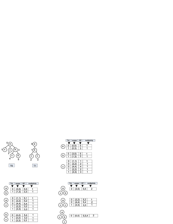
For all occurrences of a pattern that have the same , and , one occ in the occ-list of is generated and its shows the number of such occurrences. All occs of a pattern of size have as their (single vertex) rightmost paths are all different. Every occurrence is represented by exactly one occ. We refer to the occ-list of by occ-list(). It is easy to see that the frequency of is equal to . An example of occ-list is shown in Figure 5.
4.3 Operations on the occ-list data structure
Let be a tree of size generated by adding a vertex to a tree of size . There are two cases:
-
1.
is added to the rightmost vertex of . We refer to this case as leaf join.
-
2.
is added to a vertex in the rightmost path of , but not its rightmost vertex. We refer to this case as inner join.
Proposition 5 (leaf join)
Let be a one element pattern, a pattern with as the rightmost vertex, and . Let occ-list(), occ-list() and occ-list() be the representations of the occurrences of , and , respectively. We have: iff there exists an and an such that
-
()
(all occurrences are from the same database tree),
-
()
and ,
-
()
() and (i.e., copy of and an extra element),
-
()
, and
-
()
Proof
First, assume , hence it represents occurrence trees of pattern in database tree . Each of these occurrence trees share the same rightmost path. Hence they can be decomposed into occurrence trees of pattern sharing the same rightmost path and a particular occurrence of . The latter is represented by an element of occ-list(). The formers are represented by an element of occ-list(). Now we show that conditions (), …, () hold between and these elements and . Condition () holds because all occurrences are in database tree , () follows from Proposition 4, condition () follows because the rightmost path of the occurrence trees represented by is identical to that of , except for the last element which is removed, () follows from the definition of , and () holds because and represent the same number of occurrences.
Second, assume there are an and an such that conditions (), …, () hold. From () it follows that and present occurrences in the same database tree. Because () holds, if follows from Proposition 4 that all occurrence trees of represented by can be extended with into occurrence trees of ; all these occurrence trees have the same rightmost path and have as their rightmost vertex, moreover they are the only ones in the database tree with such a rightmost path. Hence, the element that satisfies properties (), …, () is indeed an element of occ-list() as has to be proven.
Figure 6 illustrates the proposition. The proposition is the basis for the operation in Algorithm 1 below.

In contrast with leaf join, which is performed between one occ of a tree pattern and one occ of a vertex, inner join is performed between a set of occs of a tree pattern and one occ of a vertex.
Proposition 6 (Inner join)
Let be a one element pattern, a pattern, a vertex on the rightmost path of but not the rightmost vertex, and . Let occ-list(), occ-list() and occ-list() be the representations of the occurrences of , and , respectively. We have: iff there exists a subset () of occ-list() and an such that
-
()
(all occurrences are from the same database tree),
-
()
, for all and for all ,
-
()
for all ,
-
()
is maximal with the conditions ()-(),
-
()
, , and (copy of part of and an extra element ),
-
()
, and
-
()
.
Proof
First, assume , hence it represents occurrence trees of pattern in database tree . All these occurrence trees share the same rightmost path. Hence, they can be decomposed into occurrence trees of pattern sharing the first vertices of the rightmost path and a particular occurrence of . The latter is represented by an element of occ-list(). The formers are represented by elements of occ-list(). Now we show that conditions (), …, () hold between and these elements and . Condition () holds because all occurrence trees are in database tree , () holds because all occurrence trees represented by share the first vertices of the rightmost paths, () and () follow from Proposition 3, () follows because the first vertices of the rightmost paths of the occurrence trees represented by are identical to those of , and the rightmost vertex of the occurrence trees represented by is the vertex represented by , () follows from the definition of , and () holds because represents occurrences.
Second, assume there are a maximal subset of and an such that conditions ((), …, () hold. From () it follows that and present occurrences in the same database tree. Because () and () hold, if follows from Proposition 3 that all occurrence trees of represented by can be extended with into occurrence trees of ; all these extended occurrence trees have the same rightmost path and have as their rightmost vertex, moreover they are the only ones in the database tree with such a rightmost path. Hence, the element that satisfies properties (), …, () is indeed an element of occ-list() as has to be proven.

4.4 Complexity analysis
Space complexity.
Given a database , space complexity of the occ-list of a pattern of size 1 is , where is the maximum number of vertices that a database tree has. For larger patterns, space complexity of the occ-list of a pattern is , where is the maximum number of occurrences with distinct rightmost paths that has in a database tree , and is the length of the rightmost path of .

Compared to data-structures generated by other algorithms such as VTreeMiner, occ-list is often substantially more compact. Given a database , the size of the data-structure generated by VTreeMiner for a pattern is , where is the maximum number of occurrences that has in a database tree and is . We note that on one hand, and the other hand, . In particular, can be significantly larger than , e.g., it can be exponentially (in terms of and ) larger than . Therefore, in the worst case, the size of the data-structure generated by VTreeMiner is exponentially larger than occ-list (and it is never smaller than occ-list). An example of this situation is shown in Figure 8. In this figure, pattern has occurrences in the database tree ( and ). If , the size of the data-structure generated by VTreeMiner will be . However, in this case, the size of the occ-list generated for is . More precisely, occ-list() has occs, where for each , , there exists an occ with , , and .

We note that there are cases where the size of occ-list (as well as the size of the data-structures used by the other algorithms) becomes exponential. An example of this situation is presented in Figure 9, where for , the size of occ-list as well as the size of scope-list used by VTreeMiner become exponential. More precisely, for each -element combination of the vertices of the database tree, there exists an occ in the occ-list of the tree pattern, where is , the lower bound of is the preorder number of the vertex with the largest depth in the combination, the upper bound of is , is an array of size filled by , and is .
In most of real-world databases, such as CSLOGS 36 and NASA Chalmers2 , while several vertices of a database tree have the same label, no two vertices on the same path are identically labeled. For trees with this property, while worst case space complexity of occ-list is linear, worst case size of scope-list remains exponential.
Time complexity.
We study time complexity of leaf join and inner join:
-
•
A leaf join between two occs takes time with the length of the rightmost path of . Since a pattern larger than 1 has occs and a pattern of size 1 has occs and leaf join is performed between every pairs of occs with the same , worst case time complexity of leaf join between two occ-lists will be .
-
•
In the inner join of the occ-lists of a tree pattern and a vertex , given an occ of , it takes time to find subsets of the occ-list of that satisfy the conditions of Proposition 6, where is the number of occs in the occ-list of . We note that occs of an occ-list can be automatically sorted first based on their s and second, based on their s. This makes it possible to find the subsets of the occ-list of that satisfy the conditions of Proposition 6 only by one scan of the occ-list of . During this scan, it is checked whether: (i) the current and the previous occs have the same , (ii) the current and the previous occs have the same , (iii) of the current occ is less than , and (iv) of the current occ is greater than or equal to . During the scan of occ-list(), after finding a subset that satisfies the conditions of Proposition 6, it takes time to perform the inner join of and . As a result, it takes time to perform the inner join of the occ-list of and an occ of . Since is and has occs, and since inner join is done between every pairs of subsets and occs that have the same s, time complexity of inner join will be .
Therefore, frequency of a pattern can be counted in time. We note that in VTreeMiner, frequency of a pattern is counted in time (recall and , in particular, it is possible that ).
4.5 A brief comparison with other vertical frequency counting approaches
As mentioned before, algorithms such as VTreeMiner 36 and MB3Miner 23 need to keep track of all occurrences. Obviously, our approach is more efficient as it simultaneously represents and processes all occurrences sharing the rightmost path in space, where is the length of the rightmost path of the pattern. TreeMinerD 36 , developed by Zaki for computing per-tree frequency, is more similar to our approach as it also processes rightmost paths of occurrences. However, there are significant differences. First, while TreeMinerD computes only per-tree frequency, our algorithm performs a much more expensive task and computes per-occurrence frequency. Second, TreeMinerD applies different join strategies.
5 TPMiner: an efficient algorithm for finding frequent embedded tree patterns
In this section, we first introduce the TPMiner algorithm and then, we discuss an optimization technique used to reduce the number of generated infrequent patterns.
5.1 The TPMiner algorithm
Having defined the operations of leaf join and inner join and having analyzed their properties, we can now introduce our tree pattern miner, called TPMiner (Tree Pattern Miner). TPMiner builds all frequent patterns and maintains the rightmost paths of all their occurrences.
TPMiner follows a depth-first strategy for generating tree patterns. First, it extracts frequent patterns of size (frequent vertex labels) and constructs their occ-lists. This step can be done by one scan of the database. Every occ of a pattern of size represents one occurrence of the pattern, where its contains the upper bound of the scope of the occurrence, its contains the scope of the occurrence, and its is . Then, larger patterns are generated using rightmost path extension. For every tree of size () which is generated by adding a vertex to a vertex on the rightmost path of a tree , the algorithm computes the occ-list of by joining the occ-lists of and . If is added to the the rightmost vertex of , a leaf join is performed; otherwise, an inner join is done. The high level pseudo code of TPMiner is given in Algorithm 1. is used to store all frequent patterns. Every tree pattern is generated in time, hence, time complexity of Algorithm 1 is , where is the number of generated candidates.
5.2 An optimization technique for candidate generation
In rightmost path extension, a new tree is generated by adding a new vertex to some vertex on the rightmost path of an existing frequent pattern , therefore, it is already known that has (at least) one frequent subtree. In an improved method proposed in 36 , to generate the tree , two patterns and such that their subtrees induced by all but the rightmost vertices are the same, are merged. In this merge, the rightmost vertex of (which is not in ) is added to as the new vertex. In this way, we already know that has (at least) two subtrees that are frequent, therefore, trees that have only one frequent subtree are not generated. This can reduce the number of trees that are generated but are infrequent.
6 Experimental Results
We performed extensive experiments to evaluate the efficiency of the proposed algorithm, using data from real applications as well as synthetic datasets. The experiments were done on one core of a single AMD Processor clocked at GHz with GB main memory and MB L2 cache, running Ubuntu Linux . The program was compiled by the GNU C++ compiler .
VTreeMiner (also called TreeMiner) 36 is a well-known algorithm for finding all frequent embedded patterns from trees. Therefore, we select this algorithm for our comparisons. Recently more efficient algorithms, such as TreeMinerD 36 , XSpanner 26 , TRIPS and TIDES 24 , have been proposed for finding frequent embedded tree patterns. However, they only compute the per-tree frequency instead of the per-occurrence frequency. Some other algorithms, such as 30 and 17 , find maximal embedded patterns which are a small subset of all frequent tree patterns. To the best of our knowledge at the time of writing this paper, MB3Miner 23 is the most efficient recent algorithm for finding frequent embedded tree patterns. MB3Miner works with both per-tree frequency and per-occurrence frequency. Here, we use the version that works with the per-occurrence frequency. We note MB3Miner generates only the frequent patterns such that all subtrees are frequent, therefore, it might produce fewer frequent patterns than VTreeMiner and TPMiner. Tatikonda et al. Tatikonda2 proposed efficient techniques for parallel mining of trees on multicore systems. Since we do not aim at parallel tree mining, their system is not proper for our comparisons.
| Dataset | # Transactions | # Vertices | # Vertex labels | Transaction size | |
|---|---|---|---|---|---|
| Maximum | Average | ||||
| CSLOGS32241 | |||||
| Prions | |||||
| NASA | |||||
We used several real-world datasets from different areas to evaluate the efficiency of TPMiner. The datasets do neither have noise nor missing values. Table 1 reports basic statistics of our real-world datasets.
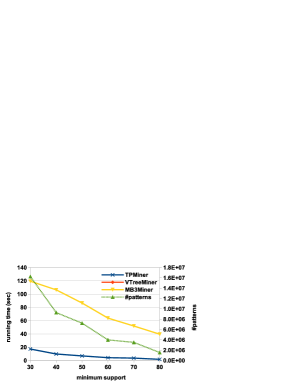
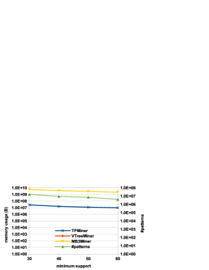
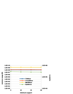
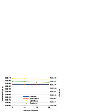
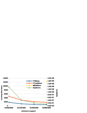
The first real-world dataset is CSLOGS 36 that contains the web access trees of the CS department of the Rensselaer Polytechnic Institute. It has trees, vertices and vertex labels. Each distinct label corresponds to the URLs of a web page. As discussed in 23 , when per-occurrence frequency is used, none of the algorithms can find meaningful patterns, because by decreasing , suddenly lots of frequent patterns with many occurrences appear in the dataset that makes the mining task practically intractable. The authors of 23 progressively reduced the dataset and generated the CSLOGS32241 dataset that contains trees. Figure 10 compares the algorithms over CSLOGS32241. For all given values of , VTreeMiner does not terminate within a reasonable time (i.e., day!), therefore, the figure does not contain it. TPMiner is faster than MB3Miner by a factor of - and it requires significantly less memory cells. In order to have a comparison with VTreeMiner, we tested the algorithms for ; while TPMiner finds frequent patterns within around seconds, VTreeMiner takes more than seconds to find the same patterns.
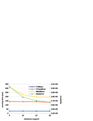
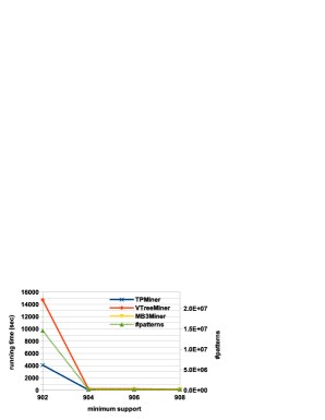
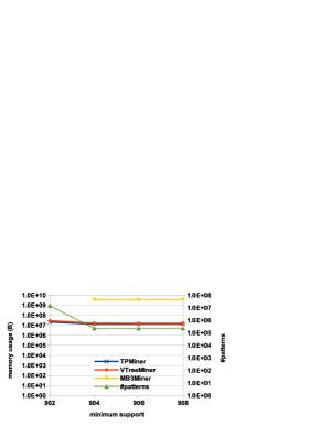
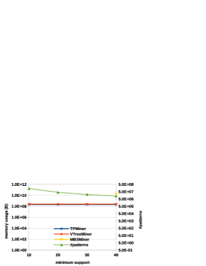
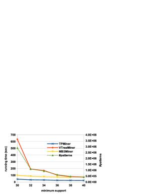
The second real-world dataset used in this paper is Prions that describes a protein ontology database for Human Prion proteins in XML format Sidhu . The authors of 23 converted it into a tree-structured dataset by considering tags as vertex labels. It has wide trees. Figure 11 reports the empirical results over this dataset, where TPMiner is faster than VTreeMiner by a factor of -, and it is faster than MB3Miner by a factor of -. The third real-world dataset is a dataset of IP multicast. The NASA dataset consists of MBONE multicast data that was measured during the NASA shuttle launch between the th and st of February, Chalmers1 and Chalmers2 . It has distinct vertex labels where each vertex label is an IP address. The data was sampled from this NASA dataset with minutes sampling interval and has trees. In this dataset, large frequent patterns are found at high minimum support values. As depicted in Figure 12, over this dataset, TPMiner is - times faster than VTreeMiner and both methods are significantly faster than MB3Miner. At , MB3Miner fails.
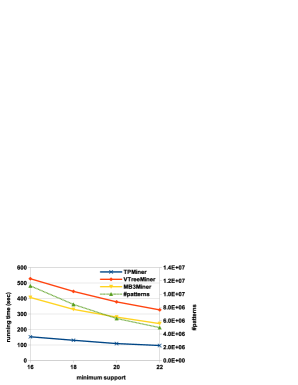
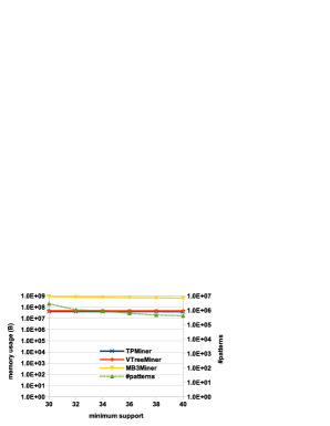
We also evaluated the efficiency of the proposed algorithm on several synthetic datasets generated by the method described in 36 . The synthetic data generation program mimics the web site browsing behavior of the user. First a master web site browsing tree is built and then the subtrees of the master tree are generated. The program is adjusted by parameters: () the number of labels (), () the number of vertices in the master tree (), () the maximum fan-out of a vertex in the master tree (), () the maximum depth of the master tree (), and () the total number of trees in the dataset (). Figure 13 compares the algorithms over the synthetic datasets. The first synthetic dataset is D10 and uses the following default values for the parameters: , , , and . Over this dataset, TPMiner is around times faster than VTreeMiner and VTreeMiner is slightly faster than MB3Miner. The next synthetic dataset is D5, where is set to and for the other parameters, the default values are used. Over this dataset, at , and , MB3Miner is aborted due to lack of memory. We also evaluated the effect of . We set to and used the default values for the other parameters and generated the M100k dataset. Over this dataset, TPMiner is faster than MB3Miner by a factor of -, and both TPMiner and MB3Miner are significantly faster than VTreeMiner.
Discussion.
Our extensive experiments report that TPMiner always outperforms well-known existing algorithms. Furthermore, there are several cases where TPMiner by order of magnitude is more efficient than any specific given algorithm. TPMiner and VTreeMiner require significantly less memory cells than MB3Miner. This is due to the different large data-structures used by MB3Miner such as the so-called EL, OC and VOL data structures and also to the breadth-first search (BFS) strategy followed by MB3Miner 23 . Although TPMiner uses a more compact representation of occurrences than VTreeMiner, this is hardly noticeable in the charts. The reason is that the memory use is dominated by the storage of the frequent patterns.
In our experiments, we can distinguish two cases. First, over datasets such as NASA and D5 (in particular for low values of ), the Tree Model Guided technique used by MB3Miner does not significantly reduce the state space, therefore, the algorithm fails or it does not terminate within a reasonable time. In such cases, TPMiner find all frequent patterns very effectively. Second, over very large datasets (such as CSLOGS32241) or dense datasets (such as M100K) where patterns have many occurrences, TPMiner becomes faster than VTreeMiner by order of magnitude. This is due to the ability of TPMiner in frequency counting of patterns with many occurrences. As discussed earlier, the occ data-structure used by TPMiner can often represent and handle exponentially many occurrences with a single occ element, while in VTreeMiner these occurrences are represented and handled one by one.
7 Conclusion
In this paper, we proposed an efficient algorithm for subtree homeomorphism with application to frequent pattern mining. We developed a compact data-structure, called occ, that effectively represents/encodes several occurrences of a tree pattern. We then defined efficient join operations on occ that help us to count occurrences of tree patterns according to occurrences of their proper subtrees. Based on the proposed subtree homeomorphism method, we introduced TPMiner, an effective algorithm for finding frequent tree patterns. We evaluated the efficiency of TPMiner on several real-world and synthetic datasets. Our extensive experiments show that TPMiner always outperforms well-known existing algorithms, and there are several situations where the improvement compared to existing algorithms is significant.
Acknowledgements.
We are grateful to Professor Mohammed Javeed Zaki for providing the VTreeMiner code, the CSLOGS datasets and the TreeGenerator program, to Dr Henry Tan for providing the MB3Miner code, to Dr Fedja Hadzic for providing the Prions dataset and to Professor Jun-Hong Cui for providing the NASA dataset. Finally, we would like to thank Dr Morteza Haghir Chehreghani for his discussion and suggestions.References
- (1) Asai, T., Abe, K., Kawasoe, S., Arimura, H., Satamoto, H., Arikawa, S.: Efficient substructure discovery from large semi-structured data. In: Proceedings of the Second SIAM International Conference on Data Mining (SDM), pp. 158–174. SIAM (2002)
- (2) Balcazar, J.L., Bifet, A., Lozano, A.: Mining frequent closed rooted trees. Machine Learning 78(1-2), 1–33 (2010)
- (3) Bille, P., Gortz, I.: The tree inclusion problem: in linear space and faster. ACM Transactions on Algorithms 7(3), 1–47 (2011)
- (4) Chalmers, R., Almeroth, K.: Modeling the branching characteristics and efficiency gains of global multicast trees. In: Proceedings of the 20th IEEE International Conference on Computer Communications (INFOCOM), pp. 449–458 (2001)
- (5) Chalmers, R.C., Member, S., Almeroth, K.C.: On the topology of multicast trees. IEEE/ACM Transactions on Networking 11, 153–165 (2003)
- (6) Chaoji, V., Hasan, M.A., Salem, S., Zaki, M.J.: An integrated, generic approach to pattern mining: data mining template library. Data Mining and Knowledge Discovery 17(3), 457–495 (2008)
- (7) Chehreghani, M.H.: Efficiently mining unordered trees. In: Proceedings of the 11th IEEE International Conference on Data Mining (ICDM), pp. 111–120 (2011)
- (8) Chehreghani, M.H., Chehreghani, M.H., Lucas, C., Rahgozar, M.: OInduced: an efficient algorithm for mining induced patterns from rooted ordered trees. IEEE Transactions on Systems, Man, and Cybernetics, Part A 41(5), 1013–1025 (2011)
- (9) Chi, Y., Muntz, R.R., Nijssen, S., Kok, J.N.: Frequent subtree mining - an overview. Fundamenta Informaticae 66(1-2), 161–198 (2005)
- (10) Chi, Y., Yang, Y., Muntz, R.R.: Indexing and mining free trees. In: Proceedings of the Third IEEE International Conference on Data Mining (ICDM), pp. 509–512 (2003)
- (11) Cui, J., Kim, J., Maggiorini, D., Boussetta, K., Gerla, M.: Aggregated multicast - a comparative study. In: Proceedings of the Second International IFIP-TC6 Networking Conference on Networking Technologies, Services, and Protocols; Performance of Computer and Communication Networks; and Mobile and Wireless Communications (NETWORKING), pp. 1032–1044 (2002)
- (12) Diestel, R.: Graph Theory, 4th ed. Springer-Verlag, Heidelberg (2010)
- (13) Dietz, P.F.: Maintaining order in a linked list. In: Proceedings of the 14th ACM Symposium on Theory of Computing (STOC), pp. 122–127 (1982)
- (14) Ivancsy, R., Vajk, I.: Frequent pattern mining in web log data. Acta Polytechnica Hungarica 3(1), 77–90 (2006)
- (15) Kilpelainen, P., Mannila, H.: Ordered and unordered tree inclusion. SIAM Journal of Computing 24(2), 340–356 (1995)
- (16) Miyahara, T., Suzuki, Y., Shoudai, T., Uchida, T., Takahashi, K., Ueda, H.: Discovery of maximally frequent tag tree patterns with contractible variables from semistructured documents. In: Proceedings of the 8th Pacific Asia Conference on Knowledge Discovery and Data Mining (PAKDD), pp. 133–144 (2004)
- (17) Nijssen, S., Kok, J.N.: Efficient discovery of frequent unordered trees. In: Proceedings of the First International Workshop on Mining Graphs, Trees, and Sequences (MGTS), pp. 55–64 (2003)
- (18) Qin, L., Yu, J.X., Ding, B.: TwigList: make twig pattern matching fast. In: Proceedings of the 12th International Conference on Database Systems for Advanced Applications (DASFAA), pp. 850–862 (2007)
- (19) Sidhu, A.S., Dillon, T.S., Chang, E.: Protein ontology. In: Z. Ma, J.Y. Chen (eds.) Database Modeling in Biology: Practices and Challenges, pp. 39–60. Springer-Verlag (2006)
- (20) Tan, H., Hadzic, F., Dillon, T.S., Chang, E., Feng, L.: Tree model guided candidate generation for mining frequent subtrees from XML documents. ACM Transaction on Knowledge Discovery from Data (TKDD) 2(2), 43 pages (2008). DOI 10.1145/1376815.1376818
- (21) Tatikonda, S., Parthasarathy, S.: Mining tree-structured data on multicore systems. The Proceedings of the VLDB Endowment (PVLDB) 2(1), 694–705 (2009)
- (22) Tatikonda, S., Parthasarathy, S., Kurc, T.M.: TRIPS and TIDES: new algorithms for tree mining. In: Proceedings of the 15th ACM International Conference on Information and Knowledge Management (CIKM), pp. 455–464 (2006)
- (23) Wang, C., Hong, M., Pei, J., Zhou, H., Wang, W., Shi, B.: Efficient pattern-growth methods for frequent tree pattern mining. In: Proceedings of the 8th Pacific Asia Conference on Knowledge Discovery and Data Mining (PAKDD), pp. 441–451 (2004)
- (24) Xiao, Y., Yao, J.F., Li, Z., Dunham, M.H.: Efficient data mining for maximal frequent subtrees. In: Proceedings of the Third IEEE International Conference on Data Mining (ICDM), pp. 379–386 (2003)
- (25) Zaki, M.J.: Efficiently mining frequent embedded unordered trees. Fundamenta Informaticae 66(1-2), 33–52 (2005)
- (26) Zaki, M.J.: Efficiently mining frequent trees in a forest: algorithms and applications. IEEE Transaction on Knowledge and Data Engineering 17(8), 1021–1035 (2005)
- (27) Zaki, M.J., Aggarwal, C.C.: XRules: an effective algorithm for structural classification of XML data. Machine Learning 62(1-2), 137–170 (2006)