Remark on Continued Fractions,
Möbius Transformations and Cycles

Abstract.

We review interrelations between continued fractions, Möbius transformations and representations of cycles by $2\times 2$ matrices. This leads us to several descriptions of continued fractions through chains of orthogonal or touching horocycles. One of these descriptions was proposed in a recent paper by A. Beardon and I. Short. The approach is extended to several dimensions in a way which is compatible to the early propositions of A. Beardon based on Clifford algebras.

1. Introduction

Continued fractions remain an important and attractive topic of current research [Khrushchev08a] [BorweinPoortenShallitZudilin14a] [Karpenkov2013a] [Kirillov06]*§ E.3. A fruitful and geometrically appealing method considers a continued fraction as an (infinite) product of linear-fractional transformations from the Möbius group. see Sec. 2 of this paper for an overview, papers [PaydonWall42a] [Schwerdtfeger45a] [PiranianThron57a] [Beardon04b] [Schwerdtfeger79a]*Ex. 10.2 and in particular [Beardon01a] contain further references and historical notes. Partial products of linear-fractional maps form a sequence in the Moebius group, the corresponding sequence of transformations can be viewed as a discrete dynamical system [Beardon01a, MageeOhWinter14a]. Many important questions on continued fractions, e.g. their convergence, can be stated in terms of asymptotic behaviour of the associated dynamical system. Geometrical generalisations of continued fractions to many dimensions were introduced recently as well [Beardon03a] [Karpenkov2013a].

Any consideration of the Möbius group introduces cycles—the Möbius invariant set of all circles and straight lines. Furthermore, an efficient treatment cycles and Möbius transformations is realised through certain $2\times 2$ matrices, which we will review in Sec. 3, see also [Schwerdtfeger79a] [Cnops02a]*§ 4.1 [FillmoreSpringer90a] [Kirillov06]*§ 4.2 [Kisil06a] [Kisil12a]. Linking the above relations we may propose the main thesis of the present note:

Claim 1.1 (Continued fractions and cycles).

Properties of continued fractions may be illustrated and demonstrated using related cycles, in particular, in the form of respective $2\times 2$ matrices.

One may expect that such an observation has been made a while ago, e.g. in the book [Schwerdtfeger79a], where both topics were studied. However, this seems did not happened for some reasons. It is only the recent paper [BeardonShort14a], which pioneered a connection between continued fractions and cycles. We hope that the explicit statement of the claim will stimulate its further fruitful implementations. In particular, Sec. 4 reveals all three possible cycle arrangements similar to one used in [BeardonShort14a]. Secs. 5–6 shows that relations between continued fractions and cycles can be used in the multidimensional case as well.

As an illustration, we draw on Fig. 1 chains of tangent horocycles (circles tangent to the real line, see [BeardonShort14a] and Sec. 4) for two classical simple continued fractions:

$$e=2+\cfrac{1}{1+\cfrac{1}{2+\cfrac{1}{1+\cfrac{1}{1+\ldots}}}}\,,\qquad\pi=3+\cfrac{1}{7+\cfrac{1}{15+\cfrac{1}{1+\cfrac{1}{292+\ldots}}}}\,.$$

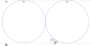
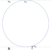
Figure 1. Continued fractions for $e$ and $\pi$ visualised. The convergence rate for $\pi$ is pictorially faster.

One can immediately see, that the convergence for $\pi$ is much faster: already the third horocycle is too small to be visible even if it is drawn. This is related to larger coefficients in the continued fraction for $\pi$.

Paper [BeardonShort14a] also presents examples of proofs based on chains of horocycles. This intriguing construction was introduced in [BeardonShort14a] ad hoc. Guided by the above claim we reveal sources of this and other similar arrangements of horocycles. Also, we can produce multi-dimensional variant of the framework.

2. Continued Fractions

We use the following compact notation for a continued fraction:

(1) $$K(a_{n}|b_{n})=\cfrac{a_{1}}{b_{1}+\cfrac{a_{2}}{b_{2}+\cfrac{a_{3}}{b_{3}+\ldots}}}=\frac{a_{1}}{b_{1}}\genfrac{}{}{0.0pt}{}{}{+}\frac{a_{2}}{b_{2}}\genfrac{}{}{0.0pt}{}{}{+}\frac{a_{3}}{b_{3}}\genfrac{}{}{0.0pt}{}{}{+\ldots}.$$

Without loss of generality we can assume $a_{j}\neq 0$ for all $j$. The important particular case of simple continued fractions, with $a_{n}=1$ for all $n$, is denoted by $K(b_{n})=K(1|b_{n})$. Any continued fraction can be transformed to an equivalent simple one.

It is easy to see, that continued fractions are related to the following linear-fractional (Möbius) transformation, cf. [PaydonWall42a, Schwerdtfeger45a, PiranianThron57a, Beardon04b]:

(2) $$S_{n}=s_{1}\circ s_{2}\circ\ldots\circ s_{n},\qquad\text{where}\quad s_{j}(z)=\frac{a_{j}}{b_{j}+z}.$$

These Möbius transformation are considered as bijective maps of the Riemann sphere $\dot{\mathbb{C}{}}=\mathbb{C}{}\cup\{\infty\}$ onto itself. If we associate the matrix $\begin{pmatrix}a&b\\ c&d\end{pmatrix}$ to a liner-fractional transformation $z\mapsto\frac{az+b}{cz+d}$, then the composition of two such transformations corresponds to multiplication of the respective matrices. Thus, relation (2) has the matrix form:

(3) $$\begin{pmatrix}P_{n-1}&P_{n}\\ Q_{n-1}&Q_{n}\end{pmatrix}=\begin{pmatrix}0&a_{1}\\ 1&b_{1}\end{pmatrix}\begin{pmatrix}0&a_{2}\\ 1&b_{2}\end{pmatrix}\cdots\begin{pmatrix}0&a_{n}\\ 1&b_{n}\end{pmatrix}.$$

The last identity can be fold into the recursive formula:

(4) $$\begin{pmatrix}P_{n-1}&P_{n}\\ Q_{n-1}&Q_{n}\end{pmatrix}=\begin{pmatrix}P_{n-2}&P_{n-1}\\ Q_{n-2}&Q_{n-1}\end{pmatrix}\begin{pmatrix}0&a_{n}\\ 1&b_{n}\end{pmatrix}.$$

This is equivalent to the main recurrence relation:

(5) $$\begin{array}[]{c}P_{n}=b_{n}P_{n-1}+a_{n}P_{n-2}\\ Q_{n}=b_{n}Q_{n-1}+a_{n}Q_{n-2}\end{array},\quad n=1,2,3,\ldots,\quad\text{with }\begin{array}[]{cc}{P_{1}}={a_{1}},&{P_{0}}=0,\\ {Q_{1}}={b_{1}},&Q_{0}=1.\end{array}$$

The meaning of entries $P_{n}$ and $Q_{n}$ from the matrix (3) is revealed as follows. Möbius transformation (2)–(3) maps $0$ and $\infty$ to

(6) $$\frac{P_{n}}{Q_{n}}=S_{n}(0),\qquad\frac{P_{n-1}}{Q_{n-1}}=S_{n}(\infty).$$

It is easy to see that $S_{n}(0)$ is the partial quotient of (1):

(7) $$\frac{P_{n}}{Q_{n}}=\frac{a_{1}}{b_{1}}\genfrac{}{}{0.0pt}{}{}{+}\frac{a_{2}}{b_{2}}\genfrac{}{}{0.0pt}{}{}{+\ldots+}\frac{a_{n}}{b_{n}}\,.$$

Properties of the sequence of partial quotients $\left\{\frac{P_{n}}{Q_{n}}\right\}$ in terms of sequences $\{a_{n}\}$ and $\{b_{n}\}$ are the core of the continued fraction theory. Equation (6) links partial quotients with the Möbius map (2). Circles form an invariant family under Möbius transformations, thus their appearance for continued fractions is natural. Surprisingly, this happened only recently in [BeardonShort14a].

3. Möbius Transformations and Cycles

If $M=\begin{pmatrix}a&b\\ c&d\end{pmatrix}$ is a matrix with real entries then for the purpose of the associated Möbius transformations $M:z\mapsto\frac{az+b}{cz+d}$ we may assume that $\det M=\pm 1$. The collection of all such matrices form a group. Möbius maps commute with the complex conjugation $z\mapsto\bar{z}$. If $\det M>0$ then both the upper and the lower half-planes are preserved; if $\det M<0$ then the two half-planes are swapped. Thus, we can treat $M$ as the map of equivalence classes $z\sim\bar{z}$, which are labelled by respective points of the closed upper half-plane. Under this identification we consider any map produced by $M$ with $\det M=\pm 1$ as the map of the closed upper-half plane to itself.

The characteristic property of Möbius maps is that circles and lines are transformed to circles and lines. We use the word cycles for elements of this Möbius-invariant family [Yaglom79, Kisil12a, Kisil06a]. We abbreviate a cycle given by the equation

(8) $$k(u^{2}+v^{2})-2lv-2nu+m=0$$

to the point $(k,l,n,m)$ of the three dimensional projective space $P\mathbb{R}^{3}{}$. The equivalence relation $z\sim\bar{z}$ is lifted to the equivalence relation

(9) $$(k,l,n,m)\sim(k,l,-n,m)$$

in the space of cycles, which again is compatible with the Möbius transformations acting on cycles.

The most efficient connection between cycles and Möbius transformations is realised through the construction, which may be traced back to [Schwerdtfeger79a] and was subsequently rediscovered by various authors [Cnops02a]*§ 4.1 [FillmoreSpringer90a] [Kirillov06]*§ 4.2, see also [Kisil06a, Kisil12a]. The construction associates a cycle $(k,l,n,m)$ with the $2\times 2$ matrix ${C}=\begin{pmatrix}l+\mathrm{i}n&-m\\ k&-l+\mathrm{i}n\end{pmatrix}$, see discussion in [Kisil12a]*§ 4.4 for a justification. This identification is Möbius covariant: the Möbius transformation defined by $M=\begin{pmatrix}a&b\\ c&d\end{pmatrix}$ maps a cycle with matrix ${C}$ to the cycle with matrix $M{C}M^{-1}$. Therefore, any Möbius-invariant relation between cycles can be expressed in terms of corresponding matrices. The central role is played by the Möbius-invariant inner product [Kisil12a]*§ 5.3:

(10) $$\left\langle{C},{\tilde{C}}\right\rangle=\Re\mathop{tr}({C}\overline{{\tilde{C}}}),$$

which is a cousin of the product used in GNS construction of $C^{*}$-algebras. Notably, the relation:

(11) $$\left\langle{C},{\tilde{C}}\right\rangle=0\quad\text{ or }\quad k\tilde{m}+m\tilde{k}-2n\tilde{n}-2l\tilde{l}=0,$$

describes two cycles ${C}=(k,l,m,n)$ and ${\tilde{C}}=(\tilde{k},\tilde{l},\tilde{m},\tilde{n})$ orthogonal in Euclidean geometry. Also, the inner product (10) expresses the Descartes–Kirillov condition [Kirillov06]*Lem. 4.1(c) [Kisil12a]*Ex. 5.26 of ${C}$ and ${\tilde{C}}$ to be externally tangent:

(12) $$\left\langle{C}+{\tilde{C}},{C}+{\tilde{C}}\right\rangle=0\quad\text{or}\quad(l+\tilde{l})^{2}+(n+\tilde{n})^{2}-(m+\tilde{m})(k+\tilde{k})=0,$$

where the representing vectors ${C}=(k,l,n,m)$ and ${\tilde{C}}=(\tilde{k},\tilde{l},\tilde{m},\tilde{n})$ from $P\mathbb{R}^{3}{}$ need to be normalised by the conditions $\left\langle{C},{C}\right\rangle=1$ and $\left\langle{\tilde{C}},{\tilde{C}}\right\rangle=1$.

4. Continued Fractions and Cycles

Let $M=\begin{pmatrix}a&b\\ c&d\end{pmatrix}$ be a matrix with real entries and the determinant $\det M$ equal to $\pm 1$, we denote this by $\delta=\det M$. As mentioned in the previous section, to calculate the image of a cycle ${C}$ under Möbius transformations $M$ we can use matrix similarity $M{C}M^{-1}$. If $M=\begin{pmatrix}P_{n-1}&P_{n}\\ Q_{n-1}&Q_{n}\end{pmatrix}$ is the matrix (3) associated to a continued fraction and we are interested in the partial fractions $\frac{P_{n}}{Q_{n}}$, it is natural to ask:

Which cycles ${C}$ have transformations $M{C}M^{-1}$ depending on the first (or on the second) columns of $M$ only?

It is a straightforward calculation with matrices to check the following statements:

Lemma 4.1.

The cycles $(0,0,1,m)$ (the horizontal lines $v=m$) are the only cycles, such that their images under the Möbius transformation $\begin{pmatrix}a&b\\ c&d\end{pmatrix}$ are independent from the column $\begin{pmatrix}b\\ d\end{pmatrix}$. The image associated to the column $\begin{pmatrix}a\\ c\end{pmatrix}$ is the horocycle $(c^{2}m,acm,\delta,a^{2}m)$, which touches the real line at $\frac{a}{c}$ and has the radius $\frac{1}{mc^{2}}$.

In particular, for the matrix (4) the horocycle is touching the real line at the point $\frac{P_{n-1}}{Q_{n-1}}=S_{n}(\infty)$ (6).

Lemma 4.2.

The cycles $(k,0,1,0)$ (with the equation $k(u^{2}+v^{2})-2v=0$) are the only cycles, such that their images under the Möbius transformation $\begin{pmatrix}a&b\\ c&d\end{pmatrix}$ are independent from the column $\begin{pmatrix}a\\ c\end{pmatrix}$. The image associated to the column $\begin{pmatrix}b\\ d\end{pmatrix}$ is the horocycle $(d^{2}k,bdk,\delta,b^{2}k)$, which touches the real line at $\frac{b}{d}$ and has the radius $\frac{1}{kd^{2}}$.

In particular, for the matrix (4) the horocycle is touching the real line at the point $\frac{P_{n}}{Q_{n}}=S_{n}(0)$ (6). In view of these partial quotients the following cycles joining them are of interest.

Lemma 4.3.

A cycle $(0,1,n,0)$ (any non-horizontal line passing $0$) is transformed by (2)–(3) to the cycle $(2Q_{n}Q_{n-1},P_{n}Q_{n-1}+Q_{n}P_{n-1},\delta n,2P_{n}P_{n-1})$, which passes points $\frac{P_{n}}{Q_{n}}=S_{n}(0)$ and $\frac{P_{n-1}}{Q_{n-1}}=S(\infty)$ on the real line.

The above three families contain cycles with specific relations to partial quotients through Möbius transformations. There is one degree of freedom in each family: $m$, $k$ and $n$, respectively. We can use the parameters to create an ensemble of three cycles (one from each family) with some Möbius-invariant interconnections. Three most natural arrangements are illustrated by Fig. 2. The first row presents the initial selection of cycles, the second row—their images after a Möbius transformation (colours are preserved). The arrangements are as follows:

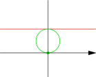
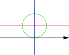
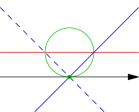
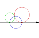
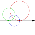
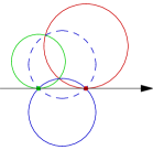
Figure 2. Various arrangements for three cycles. The first row shows the initial position, the second row—after a Möbius transformation (colours are preserved).
The left column shows the arrangement used in the paper [BeardonShort14a]: two horocycles touching, the connecting cycle is passing their common point and is orthogonal to the real line.
The central column presents two orthogonal horocycles and the connecting cycle orthogonal to them.
The horocycles in the right column are again orthogonal but the connecting cycle passes one of their intersection points and makes $45^{\circ}$ with the real axis.

1. The left column shows the arrangement used in the paper [BeardonShort14a]: two horocycles are tangent, the third cycle, which we call connecting, passes three points of pair-wise contact between horocycles and the real line. The connecting cycle is also orthogonal to horocycles and the real line. The arrangement corresponds to the following values $m=2$, $k=2$, $n=0$. These parameters are uniquely defined by the above tangent and orthogonality conditions together with the requirement that the horocycles’ radii agreeably depend from the consecutive partial quotients’ denominators: $\frac{1}{2Q_{n-1}^{2}}$ and $\frac{1}{2Q_{n}^{2}}$ respectively. This follows from the explicit formulae of image cycles calculated in Lemmas 4.1 and 4.2.

2. The central column of Fig. 2 presents two orthogonal horocycles and the connecting cycle orthogonal to them. The initial cycles have parameters $m=\sqrt{2}$, $k=\sqrt{2}$, $n=0$. Again, these values follow from the geometric conditions and the alike dependence of radii from the partial quotients’ denominators: $\frac{\sqrt{2}}{2Q_{n-1}^{2}}$ and $\frac{\sqrt{2}}{2Q_{n}^{2}}$.

3. Finally, the right column have the same two orthogonal horocycles, but the connecting cycle passes one of two horocycles’ intersection points. Its mirror reflection in the real axis satisfying (9) (drawn in the dashed style) passes the second intersection point. This corresponds to the values $m=\sqrt{2}$, $k=\sqrt{2}$, $n=\pm 1$. The connecting cycle makes the angle $45^{\circ}$ at the points of intersection with the real axis. It also has the radius $\frac{\sqrt{2}}{2}\left|\frac{P_{n}}{Q_{n}}-\frac{P_{n-1}}{Q_{n-1}}\right|=\frac{\sqrt{2}}{2}\frac{1}{\left|Q_{n}Q_{n-1}\right|}$—the geometric mean of radii of two other cycles. This again repeats the relation between cycles’ radii in the first case.

Three configurations have fixed ratio $\sqrt{2}$ between respective horocycles’ radii. Thus, they are equally suitable for the proofs based on the size of horocycles, e.g. [BeardonShort14a]*Thm. 4.1.

On the other hand, there is a tiny computational advantage in the case of orthogonal horocycles. Let we have the sequence $p_{j}$ of partial fractions $p_{j}=\frac{P_{j}}{Q_{j}}$ and want to rebuild the corresponding chain of horocycles. A horocycle with the point of contact $p_{j}$ has components $(1,p_{j},n_{j},p_{j}^{2})$, thus only the value of $n_{j}$ need to be calculated at every step. If we use the condition “to be tangent to the previous horocycle”, then the quadratic relation (12) shall be solved. Meanwhile, the orthogonality relation (11) is linear in $n_{j}$.

5. Multi-dimensional Möbius maps and cycles

It is natural to look for multidimensional generalisations of continued fractions. A geometric approach based on Möbius transformation and Clifford algebras was proposed in [Beardon03a]. The Clifford algebra ${\mathcal{C}\kern-1.30005pt\ell(n)}$ is the associative unital algebra over $\mathbb{R}{}$ generated by the elements $e_{1}$,…,$e_{n}$ satisfying the following relation:

$$e_{i}e_{j}+e_{j}e_{i}=-2\delta_{ij},$$

where $\delta_{ij}$ is the Kronecker delta. An element of ${\mathcal{C}\kern-1.30005pt\ell(n)}$ having the form $x=x_{1}e_{1}+\ldots+x_{n}e_{n}$ can be associated with vectors $(x_{1},\ldots,x_{n})\in\mathbb{R}^{n}{}$. The reversion $a\mapsto a^{*}$ in ${\mathcal{C}\kern-1.30005pt\ell(n)}$ [Cnops02a]*(1.19(ii)) is defined on vectors by $x^{*}=x$ and extended to other elements by the relation $(ab)^{*}=b^{*}a^{*}$. Similarly the conjugation is defined on vectors by $\bar{x}=-x$ and the relation $\overline{ab}=\bar{b}\bar{a}$. We also use the notation $\left|a\right|^{2}=a\bar{a}\geq 0$ for any product $a$ of vectors. An important observation is that any non-zero vectors $x$ has a multiplicative inverse: $x^{-1}=\frac{\bar{x}}{\left|x\right|^{2}}$.

By Ahlfors [Ahlfors86] (see also [Beardon03a]*§ 5 [Cnops02a]*Thm. 4.10) a matrix $M=\begin{pmatrix}a&b\\ c&d\end{pmatrix}$ with Clifford entries defines a linear-fractional transformation of $\mathbb{R}^{n}{}$ if the following conditions are satisfied:

1. $a$, $b$, $c$ and $d$ are products of vectors in $\mathbb{R}^{n}{}$;

2. $ab^{*}$, $cd^{*}$, $c^{*}a$ and $d^{*}b$ are vectors in $\mathbb{R}^{n}{}$;

3. the pseudodeterminant $\delta:=ad^{*}-bc^{*}$ is a non-zero real number.

Clearly we can scale the matrix to have the pseudodeterminant $\delta=\pm 1$ without an effect on the related linear-fractional transformation. Define, cf. [Cnops02a]*(4.7)

(13) $$\bar{M}=\begin{pmatrix}d^{*}&-b^{*}\\ -c^{*}&a^{*}\end{pmatrix}\qquad\text{ and }\qquad M^{*}=\begin{pmatrix}\bar{d}&\bar{b}\\ \bar{c}&\bar{a}\end{pmatrix}.$$

Then $M\bar{M}=\delta I$ and $\bar{M}=\kappa M^{*}$, where $\kappa=1$ or $-1$ depending either $d$ is a product of even or odd number of vectors.

To adopt the discussion from Section 3 to several dimensions we use vector rather than paravector formalism, see [Cnops02a]*(1.42) for a discussion. Namely, we consider vectors $x\in\mathbb{R}^{n+1}{}$ as elements $x=x_{1}e_{1}+\ldots+x_{n}e_{n}+x_{n+1}e_{n+1}$ in ${\mathcal{C}\kern-1.30005pt\ell(n+1)}$. Therefore we can extend the Möbius transformation defined by $M=\begin{pmatrix}a&b\\ c&d\end{pmatrix}$ with $a,b,c,d\in{\mathcal{C}\kern-1.30005pt\ell(n)}$ to act on $\mathbb{R}^{n+1}{}$. Again, such transformations commute with the reflection $R$ in the hyperplane $x_{n+1}=0$:

$$R:\quad x_{1}e_{1}+\ldots+x_{n}e_{n}+x_{n+1}e_{n+1}\quad\mapsto\quad x_{1}e_{1}+\ldots+x_{n}e_{n}-x_{n+1}e_{n+1}.$$

Thus we can consider the Möbius maps acting on the equivalence classes $x\sim R(x)$.

Spheres and hyperplanes in $\mathbb{R}^{n+1}{}$—which we continue to call cycles—can be associated to $2\times 2$ matrices [FillmoreSpringer90a] [Cnops02a]*(4.12):

(14) $$k\bar{x}x-l\bar{x}-x\bar{l}+m=0\quad\leftrightarrow\quad{C}=\begin{pmatrix}l&m\\ k&\bar{l}\end{pmatrix},$$

where $k,m\in\mathbb{R}{}$ and $l\in\mathbb{R}^{n+1}{}$. For brevity we also encode a cycle by its coefficients $(k,l,m)$. A justification of (14) is provided by the identity:

$$\begin{pmatrix}1&\bar{x}\end{pmatrix}\begin{pmatrix}l&m\\ k&\bar{l}\end{pmatrix}\begin{pmatrix}{x}\\ 1\end{pmatrix}=kx\bar{x}-l\bar{x}-x\bar{l}+m,\quad\text{ since }\bar{x}=-x\text{ for }x\in\mathbb{R}^{n}{}.$$

The identification is also Möbius-covariant in the sense that the transformation associated with the Ahlfors matrix $M$ send a cycle ${C}$ to the cycle $M{C}M^{*}$ [Cnops02a]*(4.16). The equivalence $x\sim R(x)$ is extended to spheres:

$$\begin{pmatrix}l&m\\ k&\bar{l}\end{pmatrix}\quad\sim\quad\begin{pmatrix}R(l)&m\\ k&R(\bar{l})\end{pmatrix}$$

since it is preserved by the Möbius transformations with coefficients from ${\mathcal{C}\kern-1.30005pt\ell(n)}$.

Similarly to (10) we define the Möbius-invariant inner product of cycles by the identity $\left\langle{C},{\tilde{C}}\right\rangle=\Re\mathop{tr}({C}{\tilde{C}})$, where $\Re$ denotes the scalar part of a Clifford number. The orthogonality condition $\left\langle{C},{\tilde{C}}\right\rangle=0$ means that the respective cycle are geometrically orthogonal in $\mathbb{R}^{n+1}{}$.

6. Continued fractions from Clifford algebras and horocycles

There is an association between the triangular matrices and the elementary Möbius maps of $\mathbb{R}^{n}{}$, cf. (2):

(15) $$\begin{pmatrix}0&1\\ 1&b\end{pmatrix}:\ x\ \mapsto\ (x+b)^{-1}\,,\ \text{ where }x=x_{1}e_{1}+\ldots+x_{n}e_{n},b=b_{1}e_{1}+\ldots b_{n}e_{n},$$

Similar to the real line case in Section 2, Beardon proposed [Beardon03a] to consider the composition of a series of such transformations as multidimensional continued fraction, cf. (2). It can be again represented as the the product (3) of the respective $2\times 2$ matrices. Another construction of multidimensional continued fractions based on horocycles was hinted in [BeardonShort14a]. We wish to clarify the connection between them. The bridge is provided by the respective modifications of Lem. 4.1–4.3.

Lemma 6.1.

The cycles $(0,e_{n+1},m)$ (the “horizontal” hyperplane $x_{n+1}=m$) are the only cycles, such that their images under the Möbius transformation $\begin{pmatrix}a&b\\ c&d\end{pmatrix}$ are independent from the column $\begin{pmatrix}b\\ d\end{pmatrix}$. The image associated to the column $\begin{pmatrix}a\\ c\end{pmatrix}$ is the horocycle $(-m\left|c\right|^{2},-ma\bar{c}+\delta e_{n+1},m\left|a\right|^{2})$, which touches the hyperplane $x_{n+1}=0$ at $\frac{a\bar{c}}{\left|c\right|^{2}}$ and has the radius $\frac{1}{m\left|c\right|^{2}}$.

Lemma 6.2.

The cycles $(k,e_{n+1},0)$ (with the equation $k(u^{2}+v^{2})-2v=0$) are the only cycles, such that their images under the Möbius transformation $\begin{pmatrix}a&b\\ c&d\end{pmatrix}$ are independent from the column $\begin{pmatrix}a\\ c\end{pmatrix}$. The image associated to the column $\begin{pmatrix}b\\ d\end{pmatrix}$ is the horocycle $(k\left|d\right|^{2},kb\bar{d}+\delta e_{n+1},-kb\bar{b})$, which touches the hyperplane $x_{n+1}=0$ at $\frac{b\bar{d}}{\left|d\right|^{2}}$ and has the radius $\frac{1}{k\left|d\right|^{2}}$.

The proof of the above lemmas are reduced to multiplications of respective matrices with Clifford entries.

Lemma 6.3.

A cycle ${C}=(0,l,0)$, where $l=x+re_{n+1}$ and $0\neq x\in\mathbb{R}^{n}{}$, $r\in\mathbb{R}{}$, that is any non-horizontal hyperplane passing the origin, is transformed into $M{C}M^{*}=(cx\bar{d}+d\bar{x}\bar{c},ax\bar{d}+b\bar{x}\bar{c}+\delta re_{n+1},ax\bar{b}+b\bar{x}\bar{a})$. This cycle passes points $\frac{a\bar{c}}{\left|c\right|^{2}}$ and $\frac{b\bar{d}}{\left|d\right|^{2}}$.

If $x=\bar{c}d$, then the centre of

$$M{C}M^{*}=(2\left|c\right|^{2}\left|d\right|^{2},a\bar{c}\left|d\right|^{2}+b\bar{d}\left|c\right|^{2},(a\bar{c})(d\bar{b})+(b\bar{d})(c\bar{a}))$$

is $\frac{1}{2}(\frac{a\bar{c}}{\left|c\right|^{2}}+\frac{b\bar{d}}{\left|d\right|^{2}})+\frac{\delta r}{2\left|c\right|^{2}\left|d\right|^{2}}e_{n+1}$, that is, the centre belongs to the two-dimensional plane passing the points $\frac{a\bar{c}}{\left|c\right|^{2}}$ and $\frac{b\bar{d}}{\left|d\right|^{2}}$ and orthogonal to the hyperplane $x_{n+1}=0$.

Proof.

We note that $e_{n+1}x=-xe_{n+1}$ for all $x\in\mathbb{R}^{n}{}$. Thus, for a product of vectors $d\in{\mathcal{C}\kern-1.30005pt\ell(n)}$ we have $e_{n+1}\bar{d}=d^{*}e_{n+1}$. Then

$$ce_{n+1}\bar{d}+d\bar{e}_{n+1}\bar{c}=(cd^{*}-dc^{*})e_{n+1}=(cd^{*}-(cd^{*})^{*})e_{n+1}=0,$$

due to the Ahlfors condition 2. Similarly, $ae_{n+1}\bar{b}+b\bar{e}_{n+1}\bar{a}=0$ and $ae_{n+1}\bar{d}+b\bar{e}_{n+1}\bar{c}=(ad^{*}-bc^{*})e_{n+1}=\delta e_{n+1}$.

The image $M{C}M^{*}$ of the cycle ${C}=(0,l,0)$ is $(cl\bar{d}+d\bar{l}\bar{c},al\bar{d}+b\bar{l}\bar{c},al\bar{b}+b\bar{l}{a})$. From the above calculations for $l=x+re_{n+1}$ it becomes $(cx\bar{d}+d\bar{x}\bar{c},ax\bar{d}+b\bar{x}\bar{c}+\delta re_{n+1},ax\bar{b}+b\bar{x}\bar{a})$. The rest of statement is verified by the substitution. ∎

Thus, we have exactly the same freedom to choose representing horocycles as in Section 4: make two consecutive horocycles either tangent or orthogonal. To visualise this, we may use the two-dimensional plane $V$ passing the points of contacts of two consecutive horocycles and orthogonal to $x_{n+1}=0$. It is natural to choose the connecting cycle (drawn in blue on Fig. 2) with the centre belonging to $V$, this eliminates excessive degrees of freedom. The corresponding parameters are described in the second part of Lem. 6.3. Then, the intersection of horocycles with $V$ are the same as on Fig. 2.

Thus, the continued fraction with the partial quotients $\frac{P_{n}\bar{Q}_{n}}{\left|Q_{n}\right|^{2}}\in\mathbb{R}^{n}{}$ can be represented by the chain of tangent/orthogonal horocycles. The observation made at the end of Section 4 on computational advantage of orthogonal horocycles remains valid in multidimensional situation as well.

As a further alternative we may shift the focus from horocycles to the connecting cycle (drawn in blue on Fig. 2). The part of the space $\mathbb{R}^{n}{}$ encloses inside the connecting cycle is the image under the corresponding Möbius transformation of the half-space of $\mathbb{R}^{n}{}$ cut by the hyperplane $(0,l,0)$ from Lem. 6.3. Assume a sequence of connecting cycles ${C_{j}}$ satisfies the following two conditions, e.g. in Seidel–Stern-type theorem [BeardonShort14a]*Thm 4.1:

1. for any $j$, the cycle ${C_{j}}$ is enclosed within the cycle ${C_{j-1}}$;

2. the sequence of radii of ${C_{j}}$ tends to zero.

Under the above assumption the sequence of partial fractions converges. Furthermore, if we use the connecting cycles in the third arrangement, that is generated by the cycle $(0,x+e_{n+1},0)$, where $\left\|x\right\|=1$, $x\in\mathbb{R}^{n}{}$, then the above second condition can be replaced by following

1. the sequence of $x_{n+1}^{(j)}$ of $(n+1)$-th coordinates of the centres of the connecting cycles ${C_{j}}$ tends to zero.

Thus, the sequence of connecting cycles is a useful tool to describe a continued fraction even without a relation to horocycles.

Summing up, we started from multidimensional continued fractions defined through the composition of Möbius transformations in Clifford algebras and associated to it the respective chain of horocycles. This establishes the equivalence of two approaches proposed in [Beardon03a] and [BeardonShort14a] respectively.