Space Exploration via Proximity Search

Abstract

We investigate what computational tasks can be performed on a point set in ${\mathbb{R}}^{d}$, if we are only given black-box access to it via nearest-neighbor search. This is a reasonable assumption if the underlying point set is either provided implicitly, or it is stored in a data structure that can answer such queries. In particular, we show the following:

1. One can compute an approximate bi-criteria $k$-center clustering of the point set, and more generally compute a greedy permutation of the point set.

2. One can decide if a query point is (approximately) inside the convex-hull of the point set.

We also investigate the problem of clustering the given point set, such that meaningful proximity queries can be carried out on the centers of the clusters, instead of the whole point set.

1 Introduction

Many problems in Computational Geometry involve sets of points in ${\mathbb{R}}^{d}$. Traditionally, such a point set is presented explicitly, say, as a list of coordinate vectors. There are, however, numerous applications in science and engineering where point sets are presented implicitly. This may arise for various reasons: (1) the point set (which might be infinite) is a physical structure that is represented in terms of a finite set of sensed measurements such as a point cloud, (2) the set is too large to be stored explicitly in memory, or (3) the set is procedurally generated from a highly compressed form. (A number of concrete examples are described below.)

Access to such an implicitly-represented point set $\mathsf{P}$ is performed through an oracle that is capable of answering queries of a particular type. We can think of this oracle as a black-box data structure, which is provided to us in lieu of an explicit representation. Various types of probes have been studied (such as finger probes, line probes, and X-ray probes [Ski89]). Most of these assume that $\mathsf{P}$ is connected (e.g., a convex polygon) and cannot be applied when dealing with arbitrary point sets. In this paper we consider a natural choice for probing general point sets based on computing nearest neighbors, which we call proximity probes.

More formally, we assume that the point set $\mathsf{P}$ is a (not necessarily finite) compact subset of ${\mathbb{R}}^{d}$. The point set $\mathsf{P}$ is accessible only through a nearest-neighbor data structure, which given a query point $\mathsf{q}$, returns the closest point of $\mathsf{P}$ to $\mathsf{q}$. Some of our results assume that the data structure returns an exact nearest neighbor (NN) and others assume that the data structure returns a $(1+{\varepsilon})$-approximate nearest-neighbor (ANN). (See Section 2 for definitions.) In any probing scenario, it is necessary to begin with a general notion of the set’s spatial location. We assume that $\mathsf{P}$ is contained within a given compact subset $\mathcal{D}$ of ${\mathbb{R}}^{d}$, called the domain.

The oracle is given as a black-box. Specifically, we do not allow deletions from or insertions into the data structure. We do not assume knowledge of the number of data points, nor do we make any continuity or smoothness assumptions. Indeed, most of our results apply to infinite point sets, including volumes or surfaces.

Prior Work and Applications

Implicitly-represented point sets arise in various applications. One example is that of analyzing a geometric shape through probing. An example of this is Atomic Force Microscopy (AFM) [Wik14]. This technology can reveal the undulations of a surface at the resolution of fractions of a nanometer. It relies on the principle that when an appropriately designed tip (the probe) is brought in the proximity of a surface to scan it, certain atomic forces minutely deflect the tip in the direction of the surface. Since the deflection of the tip is generally to the closest point on the surface, this mode of acquisition is an example of proximity probing. A sufficient number of such samples can be used to reconstruct the surface [BQG86].

The topic of shape analysis through probing has been well studied within the field of computational geometry. The most commonly assumed probe is a finger probe, which determines the first point of contact of a ray and the set. Cole and Yap [CY87] pioneered this area by analyzing the minimum number of finger probes needed to reconstruct a convex polygon. Since then, various alternative probing methods have been considered. For good surveys of this area, see Skiena [Ski89, Ski97].

More recently, Boissonnat et al. [BGO07] presented an algorithm for learning a smooth unknown surface $S$ bounding an object $\mathcal{O}$ in ${\mathbb{R}}^{3}$ through the use of finger probes. Under some reasonable assumptions, their algorithm computes a triangulated surface $\widehat{S}$ that approximates $S$ to a given level of accuracy. In contrast to our work, which applies to general point sets, all of these earlier results assume that the set in question is a connected shape or surface.

Implicitly-represented point sets also arise in geometric modeling. Complex geometric sets are often generated from much smaller representations. One example are fractals sets, which are often used to model natural phenomena such as plants, clouds, and terrains [SKG⁺09]. Fractal objects are generated as the limit of an iterative process [Man83]. Due to their regular, recursive structure it is often possible to answer proximity queries about such a set without generating the set itself.

Two other examples of infinite sets generated implicitly from finite models include (1) subdivision surfaces [AS10], where a smooth surface is generated by applying a recursive refinement process to a finite set of boundary points, and (2) metaballs [Bli82], where a surface is defined by a blending function applied to a collection of geometric balls. In both cases, it is possible to answer nearest neighbor queries for the underlying object without the need to generate its boundary.

Proximity queries have been applied before. Panahi et al. [PASG13] use proximity probes on a convex polygon in the plane to reconstruct it exactly. Goel et al. [GIV01], reduce the approximation versions of several problems like diameter, farthest neighbors, discrete center, metric facility location, bottleneck matching and minimum weight matching to nearest neighbor queries. They sometimes require other primitives for their algorithms, for example computation of the minimum enclosing ball or a dynamic version of the approximate nearest-neighbor oracle. Similarly, the computation of the minimum spanning tree [HIM12] can be done using nearest-neighbor queries (but the data structure needs to support deletions). For more details, see the survey by Indyk [Ind04].

Our contributions

In this paper we consider a number of problems on implicitly-represented point sets. Here is a summary of our main results.

$k$-center clustering and the greedy permutation.

Given a point set $\mathsf{P}$, a greedy permutation (informally) is an ordering of the points of $\mathsf{P}$: $\mathsf{p}_{1},\ldots,\mathsf{p}_{k},\ldots,$ such that for any $k$, the set of points $\left\{{\mathsf{p}_{1},\ldots,\mathsf{p}_{k}}\right\}$ is a $O(1)$-approximation to the optimal $k$-center clustering. This sequence arises in the $k$-center approximation of Gonzalez [Gon85], and its properties were analyzed by Har-Peled and Mendel [HM06]. Specifically, if $\mathsf{P}$ can be covered by $k$ balls of radius $r_{k}$, then the maximum distance of any point of $\mathsf{P}$ to its nearest neighbor in $\left\{{\mathsf{p}_{1},\ldots,\mathsf{p}_{k}}\right\}$ is $O(r_{k})$.

In Section 3, we show that under reasonable assumptions, in constant dimension, one can compute such an approximate greedy permutation using $O(k)$ exact proximity queries. If the oracle answers $(1+{\varepsilon})$-ANN queries, then for any $k$, the permutation generated is competitive with the optimal $k$-center clustering, considering the first $O\left({k\log_{1/{\varepsilon}}\Phi}\right)$ points in this permutation, where $\Phi$ is (roughly) the spread of the point set. The hidden constant factors grow exponentially in the dimension.

Approximate convex-hull membership.

Given a point set $\mathsf{P}$ in ${\mathbb{R}}^{d}$, we consider the problem of deciding whether a given query point $\mathsf{q}\in{\mathbb{R}}^{d}$ is inside its convex-hull $\mathcal{C}={\mathcal{CH}}\left({\mathsf{P}}\right)$. We say that the answer is ${\varepsilon}$-approximately correct if the answer is correct whenever the query point’s distance from the boundary of $\mathcal{C}$ is at least ${\varepsilon}\cdot\mathrm{d{}i{}am}\left({\mathcal{C}}\right)$. In Section 4, we show that, given an oracle for $(1+{\varepsilon}^{2}/c)$-ANN queries, for some sufficiently large constant $c$, it is possible to answer approximate convex-hull membership queries using $O(1/{\varepsilon}^{2})$ proximity queries. Remarkably, the number of queries is independent of the dimension of the data.

Our algorithm operates iteratively, by employing a gradient descent-like approach. It generates a sequence of points, all within the convex hull, that converges to the query point. Similar techniques have been used before, and are sometimes referred to as the Frank-Wolfe algorithm. Clarkson provides a survey and some new results of this type [Cla10]. A recent algorithm of this type is the work by Kalantari [Kal12]. Our main new contribution for the convex-hull membership problem is showing that the iterative algorithm can be applied to implicit point sets using nearest-neighbor queries.

Balanced proximity clustering.

We study a problem that involves summarizing a point set in a way that preserves proximity information. Specifically, given a set $\mathsf{P}$ of $n$ points in ${\mathbb{R}}^{d}$, and a parameter $k$, the objective is to select $m$ centers from $\mathsf{P}$, such that if we assign every point of $\mathsf{P}$ to its nearest center, no center has been selected by more than $k$ points. This problem is related to topic of capacitated clustering from operations research [MB84].

In Section 5, we show that in the plane there exists such a clustering consisting of $O(n/k)$ such centers, and that in higher dimensions one can select $O((n/k)\log(n/k))$ centers (where the constant depends on the dimension). This result is not directly related to the other results in the paper.

Paper organization.

In Section 2 we review some relevant work on $k$-center clustering. In Section 3 we provide our algorithm to compute an approximate $k$-center clustering. In Section 4 we show how we can decide approximately if a query point is within the convex hull of the given data points in a constant number of queries, where the constant depends on the degree of accuracy desired. Finally, in Section 5 we investigate balanced Voronoi partitions, which provides a density-based clustering of the data. Here we assume that all the data is known and the goal is to come up with a useful clustering that can help in proximity search queries.

2 Preliminaries

2.1 Background — $k$-center clustering and the greedy permutation

The following is taken from [Har11, Chap. 4], and is provided here for the sake of completeness.

In the $k$-center clustering problem, a set $\mathsf{P}\subseteq{\mathbb{R}}^{d}$ of $n$ points is provided together with a parameter $k$. The objective is to find a set of $k$ points, $\mathsf{C}\subseteq\mathsf{P}$, such that the maximum distance of a point in $\mathsf{P}$ to its closest point in $\mathsf{C}$ is minimized. Formally, define $\mathrm{price}\left({{\mathsf{C}},{\mathsf{P}}}\right)=\max_{\mathsf{p}\in\mathsf{P}}\min_{\mathsf{c}\in\mathsf{C}}\left\|{\mathsf{p}-\mathsf{c}}\right\|.$ Let $C_{\mathrm{opt}}$ denote the set of centers achieving this minimum. The $k$-center problem can be interpreted as the problem of computing the minimum radius, called the $k$-center clustering radius, such that it is possible to cover the points of $\mathsf{P}$ using $k$ balls of this radius, each centered at one of the data points. It is known that $k$-center clustering is NP-Hard. Even in the plane, it is NP-Hard to approximate to within a factor of $\left({1+\sqrt{7}}\right)/2\approx 1.82$ [FG88].

The greedy clustering algorithm.

Gonzalez [Gon85] provided a $2$-approximation algorithm for $k$-center clustering. This algorithm, denoted by GreedyKCenter, repeatedly picks the point farthest away from the current set of centers and adds it to this set. Specifically, it starts by picking an arbitrary point, $\overline{\mathrm{c}}_{1}$, and setting $\mathsf{C}_{1}=\left\{{\overline{\mathrm{c}}_{1}}\right\}$. For $i>1$, in the $i$th iteration, the algorithm computes

$$r_{i-1}=\mathrm{price}\left({{\mathsf{C}_{i-1}},{\mathsf{P}}}\right)=\max_{\mathsf{p}\in\mathsf{P}}d\left({\mathsf{p},\mathsf{C}_{i-1}}\right)$$ (2.1)

and the point $\overline{\mathrm{c}}_{i}$ that realizes it, where $d\left({\mathsf{p},\mathsf{C}_{i-1}}\right)=\min_{\mathsf{c}\in\mathsf{C}_{i-1}}\left\|{\mathsf{p}-\mathsf{c}}\right\|.$ Next, the algorithm adds $\overline{\mathrm{c}}_{i}$ to $\mathsf{C}_{i-1}$ to form the new set $\mathsf{C}_{i}$. This process is repeated until $k$ points have been collected.

If we run GreedyKCenter till it exhausts all the points of $\mathsf{P}$ (i.e., $k=n$), then this algorithm generates a permutation of $\mathsf{P}$; that is, $\left\langle{\mathsf{P}}\right\rangle=\left\langle{\overline{\mathrm{c}}_{1},\ldots,\overline{\mathrm{c}}_{n}}\right\rangle$. We will refer to $\left\langle{\mathsf{P}}\right\rangle$ as the greedy permutation of $\mathsf{P}$. There is also an associated sequence of radii $\left\langle{r_{1},\ldots,r_{n}}\right\rangle$, and the key property of the greedy permutation is that for each $i$ with $1\leq i\leq n$, all the points of $\mathsf{P}$ are within a distance at most $r_{i}$ from the points of $\mathsf{C}_{i}=\left\langle{\overline{\mathrm{c}}_{1},\ldots,\overline{\mathrm{c}}_{i}}\right\rangle$. The greedy permutation has applications to packings, which we describe next.

Definition 2.1.

A set $S\subseteq\mathsf{P}$ is an $r$-packing for $\mathsf{P}$ if the following two properties hold:

1. Covering property: All the points of $\mathsf{P}$ are within a distance at most $r$ from the points of $S$.

2. Separation property: For any pair of points $\mathsf{p},\mathsf{x}\in S$, $\left\|{\mathsf{p}-\mathsf{x}}\right\|\geq r$.

(For most purposes, one can relax the separation property by requiring that the points of $S$ be at distance $\Omega(r)$ from each other.)

Intuitively, an $r$-packing of a point set $\mathsf{P}$ is a compact representation of $\mathsf{P}$ at resolution $r$. Surprisingly, the greedy permutation of $\mathsf{P}$ provides us with such a representation for all resolutions.

Lemma 2.2 ([Har11]).

(A) Let $\mathsf{P}$ be a set of $n$ points in ${\mathbb{R}}^{d}$, and let its greedy permutation be $\langle\overline{\mathrm{c}}_{1},\ldots,$ $\overline{\mathrm{c}}_{n}\rangle$ with the associated sequence of radii $\left\langle{r_{1},\ldots,r_{n}}\right\rangle$. For any $i$, $\mathsf{C}_{i}=\left\langle{\overline{\mathrm{c}}_{1},\ldots,\overline{\mathrm{c}}_{i}}\right\rangle$ is an $r_{i}$-packing of $\mathsf{P}$. Furthermore, $r_{i}$ is a $2$-approximation for the optimal $i$-center clustering radius of $\mathsf{P}$. (B) For any $k$, let $r_{\mathrm{opt}}^{k}$ be the radius of the optimal $k$-center clustering of $\mathsf{P}$. Then, for any constant $c$, $r_{\mathrm{opt}}^{O(c^{d}k)}\leq r_{\mathrm{opt}}^{k}/c.$ (C) Computing the optimal $k$-center clustering of the first $O(k/{\varepsilon}^{d})$ points of the greedy permutation, after appropriate rescaling, results in a $(1+{\varepsilon})$-approximation to the optimal $k$-center clustering of $\mathsf{P}$.

2.2 Setup

Our algorithms operate on a (not necessarily finite) point set $\mathsf{P}$ in ${\mathbb{R}}^{d}$. We assume that we are given a compact subset of ${\mathbb{R}}^{d}$, called the domain and denoted $\mathcal{D}$, such that $\mathsf{P}\subseteq\mathcal{D}$. Throughout we assume that $\mathcal{D}$ is the unit hypercube $[0,1]^{d}$. The set $\mathsf{P}$ (not necessarily finite) is contained in $\mathcal{D}$.

Given a query point $\mathsf{q}\in[0,1]^{d}$, let $\mathrm{nn}\left({\mathsf{q},\mathsf{P}}\right)=\arg\min_{\mathsf{p}\in\mathsf{P}}\left\|{\mathsf{q}-\mathsf{p}}\right\|$ denote the nearest neighbor (NN) of $\mathsf{q}$. We say a point $\mathsf{x}$ is a $(1+{\varepsilon})$-approximate nearest-neighbor (ANN) for $\mathsf{q}$ if $\left\|{\mathsf{q}-\mathsf{x}}\right\|\leq(1+{\varepsilon})\left\|{\mathsf{q}-\mathrm{nn}\left({\mathsf{q},\mathsf{P}}\right)}\right\|$. We assume that the sole access to $\mathsf{P}$ is through “black-box” data structures $T_{nn}$ and $T_{ann}$, which given a query point $\mathsf{q}$, return the NN and ANN, respectively, to $\mathsf{q}$ in $\mathsf{P}$.

3 Using proximity search to compute $k$-center clustering

The problem.

Our purpose is to compute (or approximately compute) a $k$-center clustering of $\mathsf{P}$ through the ANN black box we have, where $k$ is a given parameter between $1$ and $n$.

3.1 Greedy permutation via NN queries: GreedyPermutNN

Let $\mathsf{q}_{0}$ be an arbitrary point in $\mathcal{D}$. Let $\nu_{0}$ be its nearest-neighbor in $\mathsf{P}$ computed using the provided NN data structure $T_{nn}$. Let $b_{0}=\mathrm{ball}\left({\mathsf{q}_{0},\left\|{\mathsf{q}_{0}-\nu_{0}}\right\|}\right)$ be the open ball of radius $\left\|{\mathsf{q}_{0}-\nu_{0}}\right\|$ centered at $\mathsf{q}_{0}$. Finally, let $G_{0}=\left\{{\nu_{0}}\right\}$, and let $\mathcal{D}_{0}=\mathcal{D}\setminus b_{0}$.

In the $i$th iteration, for $i>0$, let $\mathsf{q}_{i}$ be the point in $\mathcal{D}_{i-1}$ farthest away from $G_{i-1}$. Formally, this is the point in $\mathcal{D}_{i-1}$ that maximizes $d\left({\mathsf{q}_{i},G_{i-1}}\right)$, where $d\left({\mathsf{q},X}\right)=\min_{\mathsf{c}\in X}\left\|{\mathsf{c}-\mathsf{q}}\right\|$. Let $\nu_{i}=\mathrm{nn}\left({\mathsf{q}_{i},\mathsf{P}}\right)$ denote the nearest-neighbor $\nu_{i}$ to $\mathsf{q}_{i}$ in $\mathsf{P}$, computed using $T_{nn}$. Let

$$r_{i}=d\left({\mathsf{q}_{i},G_{i-1}}\right),\quad b_{i}=\mathrm{ball}\left({\mathsf{q}_{i},r_{i}}\right),\quad G_{i}=G_{i-1}\cup\left\{{\nu_{i}}\right\},\quad\text{and}\quad\mathcal{D}_{i}=\mathcal{D}_{i-1}\setminus b_{i}.$$

Left to its own devices, this algorithm computes a sequence of not necessarily distinct points $\nu_{0},\nu_{1},\ldots$ of $\mathsf{P}$. If $\mathsf{P}$ is not finite then this sequence may also have infinitely many distinct points. Furthermore, $\mathcal{D}_{0}\supseteq\mathcal{D}_{1}\supseteq\ldots$ is a sequence of outer approximations to $\mathsf{P}$.

The execution of this algorithm is illustrated in Figure 3.1.

(1) (2) (3) (4) (5) (6) (7) (8) (9) (10) (11) (12) (13) (14) (15) (16) Figure 3.1: An example of the execution of the algorithm GreedyPermutNN of Section 3.1.

3.2 Analysis

Let $\mathcal{O}=\left\{{o_{1},\ldots,o_{k}}\right\}$ be an optimal set of $k$ centers of $\mathsf{P}$. Formally, it is a set of $k$ points in $\mathsf{P}$ that minimizes the quantity $r_{\mathrm{opt}}^{k}=\max_{\mathsf{q}\in\mathsf{P}}d\left({\mathsf{q},\mathcal{O}}\right)$. Specifically, $r_{\mathrm{opt}}^{k}$ is the smallest possible radius such that $k$ closed balls of that radius centered at points in $\mathsf{P}$, cover $\mathsf{P}$. Our claim is that after $O(k)$ iterations of the algorithm GreedyPermutNN, the sequence of points provides a similar quality clustering of $\mathsf{P}$.

For any given point $\mathsf{p}\in{\mathbb{R}}^{d}$ we can cover the sphere of directions centered at $\mathsf{p}$ by narrow cones of angular diameter at most $\pi/12$. We fix such a covering, denoting the set of cones by $\mathcal{C}_{\mathsf{p}}$, and observe that the number of such cones is a constant $c_{d}$ that depends on the dimension. Moreover, by simple translation we can transfer such a covering to be centered at any point $\mathsf{p}^{\prime}\in{\mathbb{R}}^{d}$.

Lemma 3.1.

After $\mu=kc_{d}$ iterations, for any optimal center $o_{i}\in\mathcal{O}$, we have $d\left({o_{i},G_{\mu}}\right)\leq 3r_{\mathrm{opt}}$, where $r_{\mathrm{opt}}=r_{\mathrm{opt}}^{k}$.

Proof:

If for any $j\leq\mu$, we have $r_{j}\leq 3r_{\mathrm{opt}}$ then all the points of $\mathcal{D}_{j-1}\supseteq\mathsf{P}$ are in distance at most $3r_{\mathrm{opt}}$ from $G_{j}$, and the claim trivially holds as $\mathcal{O}\subseteq\mathsf{P}$.

Let $o$ be an optimal center and let $\mathsf{P}_{o}$ be the set of points of $\mathsf{P}$ that are closest to $o$ among all the centers of $\mathcal{O}$, i.e., $\mathsf{P}_{o}$ is the cluster of $o$ in the optimal clustering. Fix a cone $\phi$ from $\mathcal{C}_{o}$ ($\phi$’s apex is at $o$). Consider the output sequence $\nu_{0},\nu_{1},\ldots$, and the corresponding query sequence $\mathsf{q}_{0},\mathsf{q}_{1},\ldots$ computed by the algorithm. In the following, we use the property of the algorithm that $r_{1}\geq r_{2}\geq\cdots$, where $r_{i}=d\left({\mathsf{q}_{i},G_{i-1}}\right)$. A point $\mathsf{q}_{j}$ is admissible if (i) $\nu_{j}\in\mathsf{P}_{o}$, and (ii) $\mathsf{q}_{j}\in\phi$(in particular, $\nu_{j}$ is not necessarily in $\phi$).

We proceed to show that there are at most $O(1)$ admissible points for a fixed cone, which by a packing argument will imply the claim as every $\mathsf{q}_{j}$ is admissible for exactly one cone. Consider the induced subsequence of the output sequence restricted to the admissible points of $\phi$: $\nu_{1}^{\prime},\nu_{2}^{\prime},\ldots$, and let $\mathsf{q}_{1}^{\prime},\mathsf{q}_{2}^{\prime}$, $\ldots$ be the corresponding query points used by the algorithm. Formally, for a point $\nu_{i}^{\prime}$ in this sequence, let $\mathrm{iter}\left({i}\right)$ be the iteration of the algorithm it was created. Thus, for all $i$, we have $\mathsf{q}_{i}^{\prime}=\mathsf{q}_{\mathrm{iter}\left({i}\right)}$ and $\nu_{i}^{\prime}=\nu_{\mathrm{iter}\left({i}\right)}$.

Observe that $\mathsf{P}_{o}\subseteq\mathsf{P}\cap\mathrm{ball}\left({o,r_{\mathrm{opt}}}\right)$. This implies that

$$\left\|{\nu_{j}^{\prime}-o}\right\|\leq r_{\mathrm{opt}},\qquad\text{ for all }j.$$

Let $\ell_{i}^{\prime}=\left\|{\mathsf{q}_{i}^{\prime}-\nu_{i}^{\prime}}\right\|$ and $r_{i}^{\prime}=d\left({\mathsf{q}_{i}^{\prime},G_{\mathrm{iter}\left({i}\right)-1}}\right)$. Observe that for $i>1$, we have $\ell_{i}^{\prime}\leq r_{i}^{\prime}\leq\ell_{i}^{\prime}+2r_{\mathrm{opt}}$, as $\nu_{i-1}^{\prime}\in\mathsf{P}_{o}$. Hence, if $\ell_{i}^{\prime}\leq r_{\mathrm{opt}}$, then $r_{i}^{\prime}\leq 3r_{\mathrm{opt}}$, and we are done. This implies that for any $i,j$, such that $1<i<j$, it must be that $\left\|{\mathsf{q}_{i}^{\prime}-\mathsf{q}_{j}^{\prime}}\right\|\geq\ell_{i}^{\prime}>r_{\mathrm{opt}}$, as the algorithm carves out a ball of radius $\ell_{i}^{\prime}$ around $\mathsf{q}_{i}^{\prime}$, and $\mathsf{q}_{j}^{\prime}$ must be outside this ball.

By a standard packing argument, there can be only $O(1)$ points in the sequence $\mathsf{q}_{2}^{\prime},\mathsf{q}_{3}^{\prime},\ldots$ that are within distance at most $10r_{\mathrm{opt}}$ from $o$. If there are no points beyond this distance, we are done. Otherwise, let $i>1$ be the minimum index, such that $\mathsf{q}_{i}^{\prime}$ is at distance larger than $10r_{\mathrm{opt}}$ from $o$. We now prove that the points of $\phi\setminus\mathrm{ball}\left({\mathsf{q}_{i}^{\prime},\ell_{i}^{\prime}}\right)$ are of two types — those contained within $\mathrm{ball}\left({o,3r_{\mathrm{opt}}}\right)$ and those that lie at distance greater than $(4/3)\ell_{i}^{\prime}$ from $o$.

To see this, observe that since the angle of the cone was chosen to be sufficiently small, $\mathrm{ball}\left({\mathsf{q}_{i}^{\prime},\ell_{i}^{\prime}}\right)$ splits $\phi$ into two components, where all the points in the component containing $o$ are distance $<3r_{\mathrm{opt}}$ from $o$. The minimum distance to $o$ (from a point in the component not containing $o$) is realized when $\mathsf{q}_{i}^{\prime}$ is on the boundary of $\phi$ and $o$ is on the boundary of $\mathrm{ball}\left({\mathsf{q}_{i}^{\prime},\ell_{i}^{\prime}}\right)$. Then the distance of any point of $\phi\setminus\mathrm{ball}\left({\mathsf{q}_{i}^{\prime},\ell_{i}^{\prime}}\right)$ from $o$ is at least $2\ell_{i}^{\prime}\cos(\beta)\geq 2\ell_{i}^{\prime}\sqrt{3/4}\geq 1.73\ell_{i},$ as the opening angle of the cone is at most $\pi/12$. See figure on the right. The general case is somewhat more complicated as $o$ might be in distance at most $r_{\mathrm{opt}}$ from the boundary of $\mathrm{ball}\left({\mathsf{q}_{i}^{\prime},\ell_{i}^{\prime}}\right)$, but as $\ell_{i}\geq 10r_{\mathrm{opt}}$, the claim still holds — we omit the tedious but straightforward calculations.

In particular, this implies that any later point $\mathsf{q}_{k}^{\prime}$ in the sequence (i.e., $k>i$) is either one of the $O(1)$ close points, or it must be far away, but then it is easy to argue that $r_{k}^{\prime}$ must be larger than $r_{i}^{\prime}$, which is a contradiction as $r_{2}\geq r_{3}\geq\cdots$ (as $r_{i}^{\prime}$ appears before $r_{k}^{\prime}$ in this sequence).  

The above lemma readily implies the following.

Theorem 3.2.

Let $\mathsf{P}\subseteq\mathcal{D}$ be a given set of points in ${\mathbb{R}}^{d}$ (not necessarily finite), where $\mathcal{D}$ is a bounded set in ${\mathbb{R}}^{d}$. Furthermore, assume that $\mathsf{P}$ can be accessed only via a data structure $T_{nn}$ that answers exact nearest-neighbor (NN) queries on $\mathsf{P}$. The algorithm GreedyPermutNN, described in Section 3.1, computes a permutation $\left\langle{\nu_{0},\ldots}\right\rangle$ of $\mathsf{P}$, such that, for any $k>0$, $\mathsf{P}\subseteq\bigcup_{i=}^{ck}\mathrm{ball}\left({\nu_{i},r_{\mathrm{opt}}^{k}}\right),$ where $c$ is a constant (independent of $k$), and $r_{\mathrm{opt}}^{k}$ is the minimum radius of $k$ balls (of the same radius) needed to cover $\mathsf{P}$.

The algorithm can be implemented, such that running it for $i$ iterations, takes polynomial time in $i$ and involves $i$ calls to $T_{nn}$.

Proof:

Using Lemma 2.2 (B) in Lemma 3.1 implies the result. As for the running time, naively one needs to maintain the arrangement of balls inside the domain, and this can be done in polynomial time in the number of balls.  

Observation 3.3.

If $\mathsf{P}$ is finite of size $n$, the above theorem implies that after $i\geq cn$ iterations, one can recover the entire point set $\mathsf{P}$ (as $r_{\mathrm{opt}}^{n}=0$). Therefore $cn$ is an upper bound on the number of queries for any problem. Note however that in general our goal is to demonstrate when problems can be solved using a significantly smaller amount of NN queries.

The above also implies an algorithm for approximating the diameter.

Lemma 3.4.

Consider the setting of Theorem 3.2 using an exact nearest-neighbor oracle. Suppose that the algorithm is run for $m=c_{d}+1$ iterations, and let $\nu_{1},\ldots,\nu_{m}$ be the set of output centers and $r_{1},\ldots,r_{m}$ be the corresponding distances. Then, $\mathrm{d{}i{}am}\left({\mathsf{P}}\right)/3\leq\max(\mathrm{d{}i{}am}\left({\nu_{1},\ldots,\nu_{m}}\right),r_{m})\leq 3\cdot\mathrm{d{}i{}am}\left({\mathsf{P}}\right)$.

Proof:

Since the discrete one-center clustering radius lies in the interval $[\mathrm{d{}i{}am}\left({\mathsf{P}}\right)/2,\mathrm{d{}i{}am}\left({\mathsf{P}}\right)]$, Lemma 3.1 implies that $r_{m}\leq 3r_{\mathrm{opt}}\leq 3\cdot\mathrm{d{}i{}am}\left({\mathsf{P}}\right)$. Moreover, each $\nu_{i}$ is in $\mathsf{P}$, and so $\mathrm{d{}i{}am}\left({\nu_{1},\ldots,\nu_{m}}\right)\leq\mathrm{d{}i{}am}\left({\mathsf{P}}\right)$. Thus the upper bound follows.

For the lower bound, observe that if $\mathrm{d{}i{}am}\left({\nu_{1},\ldots,\nu_{m}}\right)<\mathrm{d{}i{}am}\left({\mathsf{P}}\right)/3,$ as well as $r_{m}<\mathrm{d{}i{}am}\left({\mathsf{P}}\right)/3$, then it must be true that $\mathsf{P}\subseteq\mathcal{D}_{m-1}\subseteq\bigcup_{j=1}^{l}\mathrm{ball}\left({\nu_{j},r_{m}}\right)$ has diameter less than $\mathrm{d{}i{}am}\left({\mathsf{P}}\right)$, a contradiction.  

3.3 Using approximate nearest-neighbor search

If we are using an ANN black box $T_{ann}$ to implement the algorithm, one can no longer scoop away the ball $b_{i}=\mathrm{ball}\left({\mathsf{q}_{i},\left\|{\mathsf{q}_{i}-\nu_{i}}\right\|}\right)$ at the $i$th iteration, as it might contain some of the points of $\mathsf{P}$. Instead, one has to be more conservative, and use the ball $b_{i}^{\prime}=\mathrm{ball}\left({\mathsf{q}_{i},(1-{\varepsilon})\left\|{\mathsf{q}_{i}-\nu_{i}}\right\|}\right)$ Now, we might need to perform several queries till the volume being scooped away is equivalent to a single exact query.

Specifically, let $\mathsf{P}$ be a finite set, and consider its associated spread:

$$\Phi=\frac{\mathrm{d{}i{}am}\left({\mathcal{D}_{0}}\right)}{\min_{\mathsf{p},\mathsf{x}\in\mathsf{P}}\left\|{\mathsf{p}-\mathsf{x}}\right\|}.$$

We can no longer claim, as in Lemma 3.1, that each cone would be visited only one time (or constant number of times). Instead, it is easy to verify that each query point in the cone, shrinks the diameter of the domain restricted to the cone by a factor of roughly ${\varepsilon}$. As such, at most $O\left({\log_{1/{\varepsilon}}\Phi}\right)=O\left({{\varepsilon}^{-1}\log\Phi}\right)$ query points would be associated with each cone.

Corollary 3.5.

Consider the setting of Theorem 3.2, with the modification that we use a $(1+{\varepsilon})$-ANN data structure $T_{ann}$ to access $\mathsf{P}$. Then, for any $k$, $\mathsf{P}\subseteq\bigcup_{i=1}^{f(k)}\mathrm{ball}\left({\nu_{i},r_{\mathrm{opt}}^{k}}\right),$ where $f(k)=O\left({k{\varepsilon}^{-1}\log\Phi}\right)$.

3.4 Discussion

Outer approximation.

As implied by the algorithm description, one can think about the algorithm providing an outer approximation to the set: $\mathcal{D}_{1}\supseteq\mathcal{D}_{2}\supseteq\cdots\supseteq\mathsf{P}$. As demonstrated in Figure 3.1, the sequence of points computed by the algorithm seems to be a reasonable greedy permutation of the underlying set. However, the generated outer approximation seems to be inferior. If the purpose is to obtain a better outer approximation, a better strategy may be to pick the $i$th query point $\mathsf{q}_{i}$ as the point inside $\mathcal{D}_{i}$ farthest away from $\partial\mathcal{D}_{i-1}\cup G_{i-1}$

Implementation details.

We have not spent any effort to describe in detail the algorithm of Theorem 3.2, mainly because an implementation of the exact version seems quite challenging in practice. A more practical approach would be to describe the uncovered domain $\mathcal{D}_{i}$ approximately, by approximating from the inside, every ball $b_{i}$ by an $O\left({1/{\varepsilon}^{d}}\right)$ grid of cubes, and maintaining these cubes using a (compressed) quadtree. This provides an explicit representation of the complement of the union of the approximate balls. Next, one would need to maintain for every free leaf of this quadtree, a list of points of $G_{i}$ that might serve as its nearest neighbors — in the spirit of approximate Voronoi diagrams [Har11].

4 Convex-hull membership queries via proximity queries

Let $\mathsf{P}$ be a set of $n$ points in ${\mathbb{R}}^{d}$, let $\Delta$ denote $\mathsf{P}$’s diameter, and let ${\varepsilon}>0$ be a prespecified parameter. We assume that the value of $\Delta$ is known, although a constant approximation to this value is sufficient for our purposes. (See Lemma 3.4 on how to compute this under reasonable assumptions.)

Let $\mathcal{C}={\mathcal{CH}}\left({\mathsf{P}}\right)$ denote $\mathsf{P}$’s convex hull. Given a query point $\mathsf{q}\in{\mathbb{R}}^{d}$, the task at hand is to decide if $\mathsf{q}$ is in $\mathcal{C}$. As before, we assume that our only access to $\mathsf{P}$ is via an ANN data structure. There are two possible outputs:

1. In: if $\mathsf{q}\in\mathcal{C}$, and

2. Out: if $\mathsf{q}$ is at distance greater than ${\varepsilon}\Delta$ from $\mathcal{C}$,

Either answer is acceptable if $\mathsf{q}$ lies within distance ${\varepsilon}\Delta$ of $\partial\mathcal{C}$.

4.1 Convex hull membership queries using exact extremal queries

We first solve the problem using exact extremal queries and then later show these queries can be answered approximately with ANN queries.

4.1.1 The algorithm

We construct a sequence of points $\mathsf{p}_{0},\mathsf{p}_{1},\ldots$ each guaranteed to be in the convex hull $\mathcal{C}$ of $\mathsf{P}$ and use them to determine whether $\mathsf{q}\in\mathcal{C}$. The algorithm is as follows. Let $\mathsf{p}_{0}$ be an arbitrary point of $\mathsf{P}$. For $i>0$, in the $i$th iteration, the algorithm checks whether $\left\|{\mathsf{p}_{i-1}-\mathsf{q}}\right\|\leq{\varepsilon}\Delta$, and if so the algorithm outputs In and stops.

Otherwise, consider the ray $\psi_{i}$ emanating from $\mathsf{p}_{i-1}$ in the direction of $\mathsf{q}$. The algorithm computes the point $\mathsf{z}_{i}\in\mathsf{P}$ that is extremal in the direction of this ray. If the projection $\mathsf{z}_{i}^{\prime}$ of $\mathsf{z}_{i}$ on the line supporting $\psi_{i}$ is between $\mathsf{p}_{i-1}$ and $\mathsf{q}$, then $\mathsf{q}$ is outside the convex-hull $\mathcal{C}$, and the algorithm stops and returns Out. Otherwise, the algorithm sets $\mathsf{p}_{i}$ to be the projection of $\mathsf{q}$ on the line segment $\mathsf{p}_{i-1}\mathsf{z}_{i}$, and continues to the next iteration. See figure on the right, and Figure 4.1.

The algorithm performs $O(1/{\varepsilon}^{2})$ iterations, and returns Out if it did not stop earlier.

4.1.2 Analysis

Lemma 4.1.

If the algorithm runs for more than $i$ iterations, then $\mathsf{d}_{i}<\left({1-\frac{{\varepsilon}^{2}}{2}}\right)\mathsf{d}_{i-1}$, where $\mathsf{d}_{i}=\left\|{\mathsf{q}-\mathsf{p}_{i}}\right\|$.

Proof:

By construction, $\mathsf{p}_{i}$, $\mathsf{p}_{i-1}$, and $\mathsf{q}$ form a right angle triangle. The proof now follows by a direct trigonometric argument. Consider Figure 4.1. We have the following properties:

Figure 4.1:

1. The triangles $\triangle\mathsf{p}_{i-1}\mathsf{z}_{i}^{\prime}\mathsf{z}_{i}$ and $\triangle\mathsf{p}_{i-1}\mathsf{p}_{i}\mathsf{q}$ are similar.

2. Because the algorithm has not terminated in the $i$th iteration, $\left\|{\mathsf{p}_{i-1}-\mathsf{q}}\right\|>{\varepsilon}\Delta$.

3. The point $\mathsf{q}$ must be between $\mathsf{p}_{i-1}$ and $\mathsf{z}_{i}^{\prime}$, as otherwise the algorithm would have terminated. Thus, $\left\|{\mathsf{p}_{i-1}-\mathsf{z}_{i}^{\prime}}\right\|\geq\left\|{\mathsf{p}_{i-1}-\mathsf{q}}\right\|>{\varepsilon}\Delta$.

4. We have $\left\|{\mathsf{p}_{i-1}-\mathsf{z}_{i}}\right\|\leq\Delta$, since both points are in $\mathcal{C}$.

We conclude that $\displaystyle\cos\beta=\frac{\left\|{\mathsf{p}_{i-1}-\mathsf{z}_{i}^{\prime}}\right\|}{\left\|{\mathsf{p}_{i-1}-\mathsf{z}_{i}}\right\|}>\frac{{\varepsilon}\Delta}{\Delta}={\varepsilon}.$ Now, we have

$$\left\|{\mathsf{q}-\mathsf{p}_{i}}\right\| =\left\|{\mathsf{q}-\mathsf{p}_{i-1}}\right\|\sin\beta=\left\|{\mathsf{q}-\mathsf{p}_{i-1}}\right\|\sqrt{1-\cos^{2}\beta}<\sqrt{1-{\varepsilon}^{2}}\left\|{\mathsf{q}-\mathsf{p}_{i-1}}\right\|$$

$$<\left({1-\frac{{\varepsilon}^{2}}{2}}\right)\left\|{\mathsf{q}-\mathsf{p}_{i-1}}\right\|,$$

since $(1-{\varepsilon}^{2}/2)^{2}>1-{\varepsilon}^{2}$.  

Lemma 4.2.

Either the algorithm stops within $O\left({1/{\varepsilon}^{2}}\right)$ iterations with a correct answer, or the query point is more than ${\varepsilon}\Delta$ far from the convex hull $\mathcal{C}$; in the latter case, since the algorithm says Out its output is correct.

Proof:

If the algorithm stops before it completes the maximum number of iterations, it can be verified that the output is correct as there is an easy certificate for this in each of the possible cases.

Otherwise, suppose that the query point is within ${\varepsilon}\Delta$ of $\mathcal{C}$. We argue that this leads to a contradiction; thus the query point must be more than ${\varepsilon}\Delta$ far from $\mathcal{C}$ and the output of the algorithm is correct. Observe that $\mathsf{d}_{i}$ is a monotone decreasing quantity that starts at values $\leq\Delta$ (i.e, $\mathsf{d}_{0}\leq\Delta$), since otherwise the algorithm terminates after the first iteration, as $\mathsf{z}_{1}^{\prime}$ would be between $\mathsf{q}$ and $\mathsf{p}_{0}$ on $\psi_{1}$.

Consider the $j$th epoch to be block of iterations of the algorithm, where $2^{-j}\Delta<\mathsf{d}_{i}\leq 2^{-j+1}\Delta$. Following the proof of Lemma 4.1, one observes that during the $j$th epoch one can set ${\varepsilon}_{j}=1/2^{j}$ in place of ${\varepsilon}$, and using the argument it is easy to show that the $j$th epoch lasts $O(1/{\varepsilon}_{j}^{2})$ iterations. By assumption, since the algorithm continued for the maximum number of iterations we have $\mathsf{d}_{i}>{\varepsilon}\Delta$, and so the maximum number of epochs is $\left\lceil{\lg(1/{\varepsilon})}\right\rceil$. As such, the total number of iterations is $\sum_{j=1}^{\left\lceil{\lg(1/{\varepsilon})}\right\rceil}O(1/{\varepsilon}_{j}^{2})=O(1/{\varepsilon}^{2})$. Since the algorithm did not stop this is a contradiction.  

4.1.3 Approximate extremal queries

For our purposes, approximate extremal queries on $\mathsf{P}$ are sufficient.

Definition 4.3.

A data structure provides ${\varepsilon}$-approximate extremal queries for $\mathsf{P}$, if for any query unit vector $\mathsf{v}$, it returns a point $\mathsf{p}$, such that

$$\forall\mathsf{x}\in\mathsf{P},\qquad\left\langle{{\mathsf{v}},{\mathsf{x}}}\right\rangle\leq\left\langle{{\mathsf{v}},{\mathsf{p}}}\right\rangle+{\varepsilon}\cdot\mathrm{d{}i{}am}\left({\mathsf{P}}\right),$$

where $\left\langle{{\mathsf{v}},{\mathsf{x}}}\right\rangle$ denotes the dot-product of $\mathsf{v}$ with $\mathsf{x}$.

Figure 4.2: Worse case if extremal queries are approximate.

One can now modify the algorithm of Section 4.1.1 to use, say, ${\varepsilon}/4$-approximate extremal queries on $\mathsf{P}$. Indeed, one modifies the algorithm so it stops only if $\mathsf{z}_{i}$ is on the segment $\mathsf{p}_{i-1}\mathsf{q}$, and it is in distance more than ${\varepsilon}\Delta/4$ away from $\mathsf{q}$. Otherwise the algorithm continues. It is straightforward but tedious to prove that the same algorithm performs asymptotically the same number of iterations (intuitively, all that happens is that the constants get slightly worse). The worse case as far progress in a single iteration is depicted in Figure 4.2.

Lemma 4.4.

The algorithm of Section 4.1.1 can be modified to use ${\varepsilon}/4$-approximate extremal queries and output a correct answer after performing $O\left({1/{\varepsilon}^{2}}\right)$ iterations.

4.2 Convex-hull membership via ANN queries

4.2.1 Approximate extremal queries via ANN queries

The basic idea is to replace the extremal empty half-space query, by an ANN query. Specifically, a $(1+\delta)$-ANN query performed at $\mathsf{q}$ returns us a point $\mathsf{p}$, such that

$$\forall\mathsf{x}\in\mathsf{P},\qquad\left\|{\mathsf{q}-\mathsf{p}}\right\|\leq(1+\delta)\left\|{\mathsf{q}-\mathsf{x}}\right\|.$$

Namely, $\mathrm{ball}\left({\mathsf{q},\frac{\left\|{\mathsf{q}-\mathsf{p}}\right\|}{1+\delta}}\right)$ does not contain any points of $\mathsf{P}$. Locally, a ball looks like a halfspace, and so by taking the query point to be sufficiently far and the approximation parameter to be sufficiently small, the resulting empty ball and its associated ANN can be used as the answer to an extremal direction query.

4.2.2 The modified algorithm

Assume the algorithm is given a data structure $T_{ann}$ that can answer $(1+\delta)$-ANN queries on $\mathsf{P}$. Also assume that it is provided with an initial point $\mathsf{p}_{0}\in\mathsf{P}$, and a value $\Delta^{\prime}$ that is, say, a 2-approximation to $\Delta=\mathrm{d{}i{}am}\left({\mathsf{P}}\right)$, that is $\Delta\leq\Delta^{\prime}\leq 2\Delta$.

In the $i$th iteration, the algorithm considers (again) the ray $\psi_{i}$ starting from $\mathsf{p}_{i}$, in the direction of $\mathsf{q}$. Let $\mathsf{q}_{i}$ be the point within distance, say,

$$\tau=c\Delta^{\prime}/{\varepsilon}$$ (4.1)

from $\mathsf{p}_{i-1}$ along $\psi_{i}$, where $c$ is an appropriate constant to be determined shortly. Next, let $\mathsf{z}_{i}$ be the $(1+\delta)$-ANN returned by $T_{ann}$ for the query point $\mathsf{q}_{i}$, where the value of $\delta$ would be specified shortly. The algorithm now continues as before, by setting $\mathsf{p}_{i}$ to be the nearest point on $\mathsf{p}_{i-1}\mathsf{z}_{i}$ to $\mathsf{q}$. Naturally, if $\left\|{\mathsf{q}-\mathsf{p}_{i}}\right\|$ falls below ${\varepsilon}\Delta^{\prime}/2$, the algorithm stops, and returns In, and otherwise the algorithm continues to the next iteration. As before, if the algorithm reaches the $N$th iteration, it stops and returns Out, where $N=O(1/{\varepsilon}^{2})$.

4.2.3 Analysis

Lemma 4.5.

Let $0<{\varepsilon}\leq 1$ be a prespecified parameter, and let $\delta={\varepsilon}^{2}/(32-{\varepsilon})^{2}=O({\varepsilon}^{2})$. Then, a $(1+\delta)$-ANN query done using $\mathsf{q}_{i}$ performed by the algorithm, returns a point $\mathsf{z}_{i}$ which is a valid ${\varepsilon}$-approximate extremal query on $\mathsf{P}$, in the direction of $\psi_{i}$.

Proof:

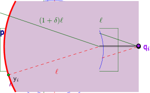
Figure 4.3: Illustration of the proof of Lemma 4.5.

Consider the extreme point $\mathsf{y}_{i}\in\mathsf{P}$ in the direction of $\psi_{i}$. Let $\mathsf{y}_{i}^{\prime}$ be the projection of $\mathsf{y}_{i}$ to the segment $\mathsf{p}_{i-1}\mathsf{q}_{i}$, and let $\ell=\left\|{\mathsf{q}_{i}-\mathsf{y}_{i}}\right\|$. See Figure 4.3.

The $(1+\delta)$-ANN to $\mathsf{q}_{i}$ (i.e., the point $\mathsf{z}_{i}$), must be inside the ball $b=\mathrm{ball}\left({\mathsf{q}_{i},(1+\delta)\ell}\right)$, and let $\mathsf{z}_{i}^{\prime}$ be its projection to the segment $\mathsf{p}_{i-1}\mathsf{q}_{i}$.

Now, if we interpret $\mathsf{z}_{i}$ as the returned answer for the approximate extremal query, then the error is the distance $\left\|{\mathsf{z}_{i}^{\prime}-\mathsf{y}_{i}^{\prime}}\right\|$, which is maximized if $\mathsf{z}_{i}^{\prime}$ is as close to $\mathsf{p}_{i-1}$ as possible. In particular, let $\mathsf{u}$ be the point in distance $(1+\delta)\ell$ from $\mathsf{q}_{i}$ along the segment $\mathsf{p}_{i-1}\mathsf{q}_{i}$. We then have that $\left\|{\mathsf{z}_{i}^{\prime}-\mathsf{y}_{i}^{\prime}}\right\|\leq h=\left\|{\mathsf{u}-\mathsf{y}_{i}^{\prime}}\right\|.$ Now, since $\left\|{\mathsf{y}_{i}^{\prime}-\mathsf{y}_{i}}\right\|\leq\left\|{\mathsf{p}_{i-1}-\mathsf{y}_{i}}\right\|\leq\Delta^{\prime}$, we have

$$h =\left\|{\mathsf{u}-\mathsf{y}_{i}^{\prime}}\right\|\leq(1+\delta)\ell-\left\|{\mathsf{y}_{i}^{\prime}-\mathsf{q}_{i}}\right\|=(1+\delta)\ell-\sqrt{\ell^{2}-\left\|{\mathsf{y}_{i}^{\prime}-\mathsf{y}_{i}}\right\|^{2}}$$

$$\leq(1+\delta)\ell-\sqrt{\ell^{2}-\left({\Delta^{\prime}}\right)^{2}}=\frac{(1+\delta)^{2}\ell^{2}-\ell^{2}+\left({\Delta^{\prime}}\right)^{2}}{(1+\delta)\ell+\sqrt{\ell^{2}-\left({\Delta^{\prime}}\right)^{2}}}\leq\frac{(2\delta+\delta^{2})\ell^{2}+\left({\sqrt{\delta}\ell}\right)^{2}}{\ell}$$

$$\leq\frac{4\delta\ell^{2}}{\ell}=4\delta\ell,$$

since $\delta\leq 1$, and assuming that $\Delta^{\prime}\leq\sqrt{\delta}\ell$. For our purposes, we need that $4\delta\ell\leq{\varepsilon}\Delta$. Both of these constraints translate to the inequalities, $\displaystyle\left({\frac{\Delta^{\prime}}{\ell}}\right)^{2}\leq\delta\leq\frac{{\varepsilon}\Delta}{4\ell}.$ Observe that, by the triangle inequality, it follows that

$$\ell=\left\|{\mathsf{q}_{i}-\mathsf{y}_{i}}\right\|\leq\left\|{\mathsf{q}_{i}-\mathsf{p}_{i-1}}\right\|+\left\|{\mathsf{p}_{i-1}-\mathsf{y}_{i}}\right\|\leq\tau+\Delta.$$

A similar argument implies that $\ell\geq\tau-\Delta$. In particular, it is enough to satisfy the constraint $\left({\frac{\Delta^{\prime}}{\tau-\Delta}}\right)^{2}\leq\delta\leq\frac{{\varepsilon}\Delta}{4(\tau+\Delta)},$ which is satisfied if $\left({\frac{\Delta^{\prime}}{\tau-\Delta^{\prime}}}\right)^{2}\leq\delta\leq\frac{{\varepsilon}\Delta^{\prime}/2}{4(\tau+\Delta^{\prime})},$ as $\Delta\leq\Delta^{\prime}\leq 2\Delta$. Substituting the value of $\tau=c\Delta^{\prime}/{\varepsilon}$, see Eq. (4.1), this is equivalent to $\left({\frac{1}{c/{\varepsilon}-1}}\right)^{2}\leq\delta\leq\frac{{\varepsilon}/2}{4(c/{\varepsilon}+1)},$ which holds for $c=32$, as can be easily verified, and setting $\delta={\varepsilon}^{2}/(32-{\varepsilon})^{2}=O({\varepsilon}^{2})$.  

Theorem 4.6.

Given a set $\mathsf{P}$ of $n$ points in ${\mathbb{R}}^{d}$, let ${\varepsilon}\in(0,1]$ be a parameter, and let $\Delta^{\prime}$ be a constant approximation to the diameter of $\mathsf{P}$. Assume that you are given a data structure that can answer $(1+\delta)$-ANN queries on $\mathsf{P}$, for $\delta=O({\varepsilon}^{2})$. Then, given a query point $\mathsf{q}$, one can decide, by performing $O(1/{\varepsilon}^{2})$ $(1+\delta)$-ANN queries whether $\mathsf{q}$ is inside the convex-hull $\mathcal{C}={\mathcal{CH}}\left({\mathsf{P}}\right)$. Specifically, the algorithm returns

• In: if $\mathsf{q}\in\mathcal{C}$, and

• Out: if $\mathsf{q}$ is more than ${\varepsilon}\Delta$ away from $\mathcal{C}$, where $\Delta=\mathrm{d{}i{}am}\left({\mathsf{P}}\right)$.

The algorithm is allowed to return either answer if $\mathsf{q}\notin\mathcal{C}$, but the distance of $\mathsf{q}$ from $\mathcal{C}$ is at most ${\varepsilon}\Delta$.

5 Density clustering

5.1 Definition

Given a set $\mathsf{P}$ of $n$ points in ${\mathbb{R}}^{d}$, and a parameter $k$ with $1\leq k\leq n$, we are interested in computing a set $\mathsf{C}\subseteq\mathsf{P}$ of “centers”, such that each center is assigned at most $k$ points, and the number of centers is (roughly) $n/k$. In addition, we require that:

1. A point of $\mathsf{P}$ is assigned to its nearest neighbor in $\mathsf{C}$ (i.e., $\mathsf{C}$ induces a Voronoi partition of $\mathsf{P}$).

2. The centers come from the original point set.

Intuitively, this clustering tries to capture the local density — in areas where the density is low, the clusters can be quite large (in the volume they occupy), but in regions with high density the clusters have to be tight and relatively “small”.

Formally, given a set of centers $\mathsf{C}$, and a center $\mathsf{c}\in\mathsf{C}$, its cluster is

$$\mathsf{P}_{\mathsf{c}}=\left\{\mathsf{p}\in\mathsf{P}\;\middle|\;\bigl{.}\left\|{\mathsf{c}-\mathsf{p}}\right\|<d\left({\mathsf{p},\mathsf{C}\setminus\left\{{c}\right\}\bigr{.}}\right)\Bigl{.}\right\},$$

where $d\left({\mathsf{c},X}\right)=\min_{\mathsf{p}\in X}\left\|{\mathsf{c}-\mathsf{p}}\right\|$ (and assuming for the sake of simplicity of exposition that all distances are distinct). The resulting clustering is $\mathrm{\Pi}\left({\mathsf{P},\mathsf{C}}\right)=\left\{{\mathsf{P}_{\mathsf{c}}\,\left|\,{\mathsf{c}\in\mathsf{C}}\right.}\right\}$. A set of points $\mathsf{P}$, and a set of centers $\mathsf{C}\subseteq\mathsf{P}$ is a $k$-density clustering of $\mathsf{P}$ if for any $\mathsf{c}\in\mathsf{C}$, we have $\left|{\mathsf{P}_{\mathsf{c}}}\right|\leq k$. As mentioned, we want to compute a balanced partitioning, i.e., one where the number of centers is roughly $n/k$. We show below that this is not always possible in high enough dimensions.

5.1.1 A counterexample in high dimension

Lemma 5.1.

For any integer $n>0$, there exists a set $\mathsf{P}$ of $n$ points in ${\mathbb{R}}^{n}$, such that for any $k<n$, a $k$-density clustering of $\mathsf{P}$ must use at least $n-k+1$ centers.

Proof:

Let $n$ be a parameter. For $i=1,\ldots,n$, let $\ell_{i}=\sqrt{1-2^{-i-1}}$, and let $\mathsf{p}_{i}$ be a point of ${\mathbb{R}}^{n}$ that has zero in all coordinates except he $i$th one, where its value is $\ell_{i}$. Let $\mathsf{P}=\left\{{\mathsf{p}_{1},\ldots,\mathsf{p}_{n}}\right\}\subseteq{\mathbb{R}}^{n}$. Now, $d_{i,j}=\left\|{\mathsf{p}_{i}-\mathsf{p}_{j}}\right\|=\sqrt{\ell_{i}^{2}+\ell_{j}^{2}}=\sqrt{2-2^{-i-1}-2^{-j-1}}$. For $i<j$ and $i^{\prime}<j^{\prime}$, we have

$$d_{i,j}<d_{i^{\prime},j^{\prime}} \iff 2-2^{-i-1}-2^{-j-1}<2-2^{-i^{\prime}-1}-2^{-j^{\prime}-1}\iff 2^{-i^{\prime}}+2^{-j^{\prime}}<2^{-i}+2^{-j}$$

$$\iff\begin{cases}i=i^{\prime}\text{ and }j<j^{\prime},or\\ i<i^{\prime}.\end{cases}$$

That is, the distance of the $i$th point to all the following points $\mathsf{S}_{i+1}=\left\{{\mathsf{p}_{i+1},\ldots,\mathsf{p}_{n}}\right\}$ is smaller than the distance between any pair of points of $\mathsf{S}_{i+1}$.

Now, consider any set of centers $\mathsf{C}\subseteq\mathsf{P}$, and let $\mathsf{c}=\mathsf{p}_{i}$ be the point with the lowest index that belongs to $\mathsf{C}$. Clearly, $\mathsf{P}_{\mathsf{c}}=\left({\mathsf{P}\setminus\mathsf{C}}\right)\cup\left\{{\mathsf{c}}\right\}$; that is, all the non-center points of $\mathsf{P}$, get assigned by the clustering to $\mathsf{c}$, implying what we want to show.  

5.2 Algorithms

5.2.1 Density clustering via nets

Lemma 5.2.

For any set of $n$ points $\mathsf{P}$ in ${\mathbb{R}}^{d}$, and a parameter $k<n$, there exists a $k$-density clustering with $O\left({\frac{n}{k}\log\frac{n}{k}}\right)$ centers (the $O$ notation hides constants that depend on $d$).

Proof:

Consider the hypercube $[-1,1]^{d}$. Cover its outer faces (which are $(d-1)$-dimensional hypercubes) by a grid of side length $1/3\sqrt{d}$. Consider a cell $C$ in this grid — it has diameter $\leq 1/3$, and it is easy to verify that the cone $\phi_{C}=\left\{t\mathsf{p}\;\middle|\;\mathsf{p}\in C,t\geq 0\right\}$ formed by the origin and $C$ has angular diameter $<\pi/3$. This results in a set $\mathcal{C}$ of $N=O(d^{d})$ cones covering ${\mathbb{R}}^{d}$.

Furthermore, the cone $\phi_{C}$ is formed by the intersection of $2(d-1)$ halfspaces. As such, the range space consisting of all translations of $\phi_{C}$ has VC dimension at most $d^{\prime}=O(d^{2}\log d)$ [Har11, Theorem 5.22]. Let slice be the set that is formed by the intersection of such a cone, with a ball centered at its apex. The range space of such slices has VC dimension $d^{\prime\prime}=O(d+2+d^{\prime})=O(d^{2}\log d)$, since the VC dimension of balls in ${\mathbb{R}}^{d}$ is $d+2$, and one can combine the range spaces as done above, see the book [Har11] for background on this.

Now, for ${\varepsilon}=(k/N)/n$, consider an ${\varepsilon}$-net $\mathsf{R}$ of the point set $\mathsf{P}$ for slices. The size of such a net is $\left|{\mathsf{R}}\right|=O\left({(d^{\prime\prime}/{\varepsilon})\log{\varepsilon}^{-1}}\right)=d^{O(d)}(n/k)\log(n/k)$.

Consider a point $\mathsf{p}\in\mathsf{P}$ that is in $\mathsf{R}$, and consider the cones of $\mathcal{C}$ translated so that their apex is $\mathsf{p}$. For a cone $\phi\in\mathcal{C}$, let $\nu_{\phi}$ be the nearest point to $\mathsf{p}$ in the set $\left\{{\mathsf{R}\setminus\left\{{\mathsf{p}}\right\}\Bigl{.}}\right\}\cap\phi$. The key observation is that any point in $\mathsf{P}\cap\phi$ that is farther away from $\mathsf{p}$ than $\nu_{\phi}$, is closer to $\nu_{\phi}$ than to $\mathsf{p}$; that is, only points closer to $\mathsf{p}$ than $\nu_{\phi}$ might be assigned to $\mathsf{p}$ in the Voronoi clustering. Since $\mathsf{R}$ is an ${\varepsilon}$-net for slices, the slice $\mathrm{ball}\left({\bigl{.}\mathsf{p},\left\|{\mathsf{p}-\nu_{\phi}}\right\|}\right)\cap\phi$ contains at most ${\varepsilon}n=k/N$ points of $\mathsf{P}$. It follows that at most $k/N$ points of $\mathsf{P}\cap\phi$ are assigned to the cluster associated with $\mathsf{p}$. By summing over all $N$ cones, at most $(k/N)N=k$ points are assigned to $\mathsf{p}$, as desired.  

5.2.2 The planar case

Lemma 5.3.

For any set of $n$ points $\mathsf{P}$ in ${\mathbb{R}}^{2}$, and a parameter $k$ with $1\leq k\leq n$, there exists a $k$-density clustering with $O\left({n/k}\right)$ centers.

Proof:

Consider the plane, and a cone $\phi\in\mathcal{C}$ as used in the proof of Lemma 5.2. For a point $\mathsf{p}\in{\mathbb{R}}^{2}$, and a radius $r$, let $\phi_{\mathsf{p}}$ denote the translated cone having $\mathsf{p}$ as an apex, and let $s(\mathsf{p},r)=\phi_{\mathsf{p}}\cap\mathrm{ball}\left({\mathsf{p},r}\right)$ be a slice induced by this cone. Consider the set of all possible slices in the plane:

$$S=\left\{s(\mathsf{p},r)\;\middle|\;\mathsf{p}\in{\mathbb{R}}^{2},r\geq 0\right\}.$$

It is easy to verify that the family $S$ behaves like a system of pseudo-disks; that is, the boundary of a pair of such regions intersects in at most two points, see figure on the right. As such, the range space having $\mathsf{P}$ as the ground set, and $S$ as the set of possible ranges, has an ${\varepsilon}$-net of size $O(1/{\varepsilon})$ [MSW90]. Let ${\varepsilon}=(k/N)/n$, as in the proof of Lemma 5.2, where $N=\left|{\mathcal{C}}\right|$. Computing such an ${\varepsilon}$-net, for every cone of $\mathcal{C}$, and taking their union results in the desired set of cluster centers.

References

- [AS10] L.-E. Andersson and N. F. Stewart. Introduction to the Mathematics of Subdivision Surfaces. SIAM, 2010.
- [BGO07] J.-D. Boissonnat, L. J. Guibas, and S. Oudot. Learning smooth shapes by probing. Comput. Geom. Theory Appl., 37(1):38–58, 2007.
- [Bli82] J. F. Blinn. A generalization of algebraic surface drawing. ACM Trans. Graphics, 1:235–256, 1982.
- [BQG86] G. Binnig, C. F. Quate, and Ch. Gerber. Atomic force microscope. Phys. Rev. Lett., 56:930–933, Mar 1986.
- [Cla10] K. L. Clarkson. Coresets, sparse greedy approximation, and the frank-wolfe algorithm. ACM Trans. Algo., 6(4), 2010.
- [CY87] R. Cole and C. K. Yap. Shape from probing. J. Algorithms, 8(1):19–38, 1987.
- [FG88] T. Feder and D. H. Greene. Optimal algorithms for approximate clustering. In Proc. 20th Annu. ACM Sympos. Theory Comput. (STOC), pages 434–444, 1988.
- [GIV01] A. Goel, P. Indyk, and K. R. Varadarajan. Reductions among high dimensional proximity problems. In Proc. 12th ACM-SIAM Sympos. Discrete Algs. (SODA), pages 769–778, 2001.
- [Gon85] T. Gonzalez. Clustering to minimize the maximum intercluster distance. Theoret. Comput. Sci., 38:293–306, 1985.
- [Har11] S. Har-Peled. Geometric Approximation Algorithms, volume 173 of Mathematical Surveys and Monographs. Amer. Math. Soc., 2011.
- [HIM12] S. Har-Peled, P. Indyk, and R. Motwani. Approximate nearest neighbors: Towards removing the curse of dimensionality. Theory Comput., 8:321–350, 2012. Special issue in honor of Rajeev Motwani.
- [HM06] S. Har-Peled and M. Mendel. Fast construction of nets in low dimensional metrics, and their applications. SIAM J. Comput., 35(5):1148–1184, 2006.
- [Ind04] P. Indyk. Nearest neighbors in high-dimensional spaces. In J. E. Goodman and J. O’Rourke, editors, Handbook of Discrete and Computational Geometry, chapter 39, pages 877–892. CRC Press LLC, 2nd edition, 2004.
- [Kal12] B. Kalantari. A characterization theorem and an algorithm for A convex hull problem. CoRR, abs/1204.1873, 2012.
- [Man83] B. B. Mandelbrot. The fractal geometry of nature. Macmillan, 1983.
- [MB84] J. M. Mulvey and M. P. Beck. Solving capacitated clustering problems. Euro. J. Oper. Res., 18:339–348, 1984.
- [MSW90] J. Matoušek, R. Seidel, and E. Welzl. How to net a lot with little: Small -nets for disks and halfspaces. In Proc. 6th Annu. Sympos. Comput. Geom. (SoCG), pages 16–22, 1990.
- [PASG13] F. Panahi, A. Adler, A. F. van der Stappen, and K. Goldberg. An efficient proximity probing algorithm for metrology. In Proc. IEEE Int. Conf. Autom. Sci. Engin. (CASE), pages 342–349, 2013.
- [SKG+09] R. M. Smelik, K. J. De Kraker, S. A. Groenewegen, T. Tutenel, and R. Bidarra. A survey of procedural methods for terrain modelling. In Proc. of the CASA Work. 3D Adv. Media Gaming Simul., 2009.
- [Ski89] S. S. Skiena. Problems in geometric probing. Algorithmica, 4:599–605, 1989.
- [Ski97] S. S. Skiena. Geometric reconstruction problems. In J. E. Goodman and J. O’Rourke, editors, Handbook of Discrete and Computational Geometry, chapter 26, pages 481–490. CRC Press LLC, Boca Raton, FL, 1997.
- [Wik14] Wikipedia. Atomic force microscopy — wikipedia, the free encyclopedia, 2014.