Iterative Splitting Methods: Almost Asymptotic Symplectic Integrator for Stochastic Nonlinear Schrödinger Equation
Jürgen Geiser
University of Greifswald, Institute of Physics, Felix-Hausdorff-Str. 6, D-17489 Greifswald, Germany, E-mail: jgeiser@uni-greifswald.de
Abstract
In this paper we present splitting methods which
are based on iterative schemes and
applied to stochastic nonlinear Schrödinger equation.
We will design stochastic integrators
which almost conserve the symplectic structure.
The idea is based on rewriting an iterative splitting
approach as a successive approximation method based on
a contraction mapping principle and that we have an almost
symplectic scheme, see [12] and [9].
We apply a stochastic differential equation, that we can
decouple into a deterministic and stochatic part, while
each part can be solved analytically.
Such decompositions allow accelerating the methods and preserving, under
suitable conditions, the symplecticity of the schemes.
A numerical analysis and application to the stochastic Schrödunger equation are presented.
The motivation is to develop fast solver schemes to
solve stochastic Hamiltonians in solitary waves and collisions.
The idea is based on almost asymptotic symplecticity for
stochastic Hamiltonian partial differential equations,
such underlying algorithms are applied to develop
stochastic symplectic methods
for solving a stochastic Schroedinger equations, see [12].
It is shown that the noval schemes preserve the symplectic structure
in an asymptotic regime, which means it is away from
a symplectic scheme with .
Definition 1.1.
We consider a Hamiltonian system, while and we write:
(1)
where and and is the d-dimensional identity matrix,
is the gradient with respect to .
We assume that is the solution operator with , where isthe time step and we have the following definition about the symplecticity:
•
preserves the symplecticness of the system (1), if:
(2)
•
preserves the almost (or asymptotic) symplecticness of the system (1), if:
(3)
where is a constant with and is a function of , which is given from the solution method.
Remark 1.1.
The idea of almost symplecticity has the origin of
modifying the definition of symplecticity.
For example, if one assume that depends on , then
one can proof, that we have an almost poisson structure
and we preserve the poisson structure up to the second order,
see [2].
Such ideas are also used in the development in pseudo-symplectic methods, see [1].
In the following, we deal with the stochastic nonlinear Schrödinger equation with multiplicative noise, which is given by
(4)
where is the complex-valued solution and denotes
is defined as a real-valued white noise which is delta correlated in time and either smooth or delta correlated in space.
The deterministic nonlinear Schroedinger equation is given by
2 Iterative Splitting as a Successive Approximation Method
We can rewrite this to a Hamiltonian system by
, where and are real-valued functions and we can separate it into the following form and we obtain a multi-symplectic system:
(10)
where we have the symplectic structure .
The system is given by
(22)
where the matrices are given by the semi-discretization of the original system
(4).
Theorem 2.1.
The iterative splitting scheme is almost symplectic.
Proof.
For the Hamiltonian system
(23)
we apply the successive approximation method:
(24)
where we apply the linearised scheme:
(25)
further, the contraction mapping is given by
(26)
where and
and .
∎
3 Almost Symplectic Scheme
In the following, we discuss the linearised equation
in the algorithm.
We have the fixed-splitting discretisation step-size , on the
time-interval , and the stochastic time step (Wiener process), where is a Gaussian distributed
random variable with and , see [10].
We solve the following sub-problems
consecutively for . (cf. [4]):
(27)
where is the known successive approximation at the
time-level . The split approximation at the time-level
is defined by .
We can rewrite this into the following ODE form:
(28)
where .
Theorem 3.1.
We are given linear bounded operators
(e.g., due to the linearisation) and we consider the abstract Cauchy problem
(29)
Then the problem (29) has a unique solution; the iterations
(28) over are convergent with order .
Furthermore, the almost asymptotic symplecticity of the scheme (28)
is given as:
Theorem 3.2.
Consider the algorithm (28) and let be the
solver step of the algorithm.
Then for any , there exists , where and the time-step , where is the number of iterative steps,
and we have
In the following, we treat the different numerical methods.
The underlying equation is given as
(40)
where the initial values are given as ,
and is a Wiener process.
We apply a semi-discretisation via finite difference schemes and obtain the
ODE problem
(41)
where the operators are given by
(42)
(43)
(44)
where we apply the different splitting schemes.
4.1 Linearised stochastic Schroedinger equation
We consider the following linearised stochastic Schroedinger equation:
(45)
(46)
(47)
where .
We assume periodic boundary conditions ,
where , e.g. , and is small.
We employ the following transformation and change of variables:
(54)
We apply a finite difference discretisation and the matrices are
given as
(55)
(56)
(57)
(58)
(64)
(70)
(71)
(77)
where we have , , .
We apply the operator splitting schemes:
(80)
(85)
where , the random variable is based on a Wiener process with , and
is a Gaussian distributed random variable with and
. This means we have .
The splitting operators are
(88)
(91)
(94)
We present the different convergent time-steps results
for .
The analytical solution is
We apply the operator splitting schemes as follows:
(97)
(100)
(101)
where , the random variable is based on a Wiener process with , and
is a Gaussian distributed random variable with and
. This means we have .
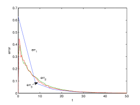
The solution is given by and the errors are
(103)
In the following figures, we present the results for the error
of the iterative splitting schemes, see Fig. 1.
Figure 1: The -errors of the iterative
splitting scheme
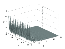
In the following figures, we present the results for the
different splitting schemes, see Fig. 2.
Figure 2: The results of the A–B splitting with .
Remark 4.1.
With more iterative steps, we see an improvement in the numerical results.
With two to three iterative steps, we obtain nearly the analytical solution.
Here, we could see the almost asymptotic behaviour of the scheme.
We employ the following transformation and change of variables:
(112)
(113)
(114)
(115)
The underlying discretised matrices for the splitting schemes are given as:
(118)
(119)
(122)
In the next list of schemes we discuss different splitting scheme.
The first splitting scheme is known as an A-B splitting or Lie-Trotter splitting scheme, see [13], while we apply multiplicative the different separated operators. The second splitting scheme is known as an iterative splitting scheme,
see [5]. Such a scheme apply iteratively the separated operators based on
a fix-point approximation, see [7].
We will employ the following splitting schemes:
•
A–B splitting
(123)
•
Strang splitting scheme
(124)
•
Weighted Iterative Splitting 1:
We define a relaxed iterative splitting method based on the critical value :
(125)
(126)
and , and .
The algorithm is
(127)
(128)
(129)
(130)
and is solved as:
(131)
(132)
(133)
where the given is defined as:
(134)
(135)
(136)
•
Weighted Iterative Splitting 2:
We define a relaxed iterative splitting method based on the critical value :
(137)
(138)
(139)
where is the known split
approximation at the time level . The split
approximation at the time level is defined as
. The parameter . For
, we have the sequential splitting
method, and for we have the iterative splitting method.
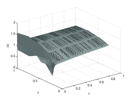
The following figures present the results for the
different splitting schemes, see Fig. 3.
Figure 3: Results of the iterative splitting approach.
Remark 4.2.
Here, we have compared the standard splitting scheme with our iterative
splitting approach. Based on the resolution of the analytical solution,
we obtain the same results as for the standard schemes.
4.3 Deterministic nonlinear Schrödinger equation
We consider the equation
(140)
(141)
with and .
We choose the initial condition:
(142)
Then the exact single-soliton solution is
(143)
We employ the following transformation and change of variables:
(150)
(151)
(152)
(153)
The underlying discretised matrices for the splitting schemes are
(156)
(157)
(160)
We consider the following splitting schemes:
•
A–B splitting
(161)
•
Strang splitting scheme
(162)
•
Weighted Iterative Splitting 1:
We define a relaxed iterative splitting method based on the critical value :
(163)
(164)
and , and .
The algorithm is
(165)
(166)
(167)
(168)
and is solved as
(169)
(170)
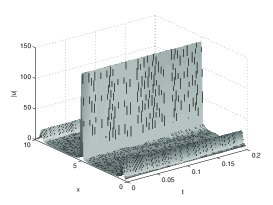
The following figures present the results for the
different splitting schemes, see Fig. 4.
Figure 4: Results of the iterative splitting approach.
We apply for each solution and obtain the following errors:
(171)
(172)
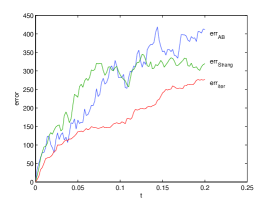
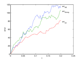
The following figures present the results for the errors
of the iterative splitting schemes, see Fig. 5.
Figure 5: The -errors of the different splitting schemes, where in the left figure, we have and and in the right figure, we have and .
Remark 4.3.
In both resolution in time and space the iterative splitting method is
more accurate than the standard A–B and Strang splitting schemes.
Here, we see an improvement based on the successive approximation idea
and obtain a more accurate linearisation than for the standard schemes.
4.4 Stochastic nonlinear Schrödinger equation
We consider the equation
(173)
(174)
with and .
We choose the initial condition
(175)
For the reference solution, we apply a fine resolution Strang splitting.
We employ the following transformation and change of variables:
(182)
(183)
(184)
(185)
(186)
The underlying discretised matrices for the splitting schemes are
(190)
(191)
(194)
(197)
and
(198)
•
A–B splitting
We apply the operator splitting schemes as:
(201)
(202)
(205)
(206)
(207)
where , the random variable is based on a Wiener process with , and
is a Gaussian distributed random variable with and
. This means we have .
•
Iterative splitting scheme:
First iterative step
(212)
Second iterative step
The stochastic integral is computed as a Stratonovich integral:
(215)
We apply for each solution and deal with the following errors:
(216)
(217)
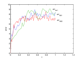
The following figures present the results for the error
of the iterative splitting schemes, see Fig. 6.
Figure 6: The -errors of the different splitting scheme, where we compare them to the solution obtained from a fine resolution iterative splitting scheme
Remark 4.4.
In both resolution in time and space the iterative splitting method is
more accurate than the standard A–B and Strang splitting schemes.
Here, we obtain an improvement based on the successive approximation
scheme.
5 Conclusion
We discuss the problems of using novel iterative splitting schemes
to solve stochastic nonlinear Schroedinger equations.
We could prove the almost asymptotic symplectic behaviour of the novel scheme.
The improvement with more iterative steps allows resolving the nonlinearity
and obtaining an improved symplectic scheme.
While standard splitting schemes have drawbacks as regards linearisation
and symplecticity, we could derive a combination of both higher accuracy and
conservation of the symplecticity.
In the future, we will take into account larger equation systems for
a realistic application.
References
[1]
A. Aubry and P. Chartier.
Pseudo-symplectic Runge-Kutta methods.BIT, 38:439-461, 1998.
[2]
M.A. Austin, P.S. Krishnaprasad, and L. Wang.
Almost Poisson integration of rigid body systems.Journal of Comput. Phys., 107, 105-117, 1993.
[3]
J. Geiser.
Numerical Simulation of a Model for Transport and Reaction of Radionuclides.
Proceedings of the Large Scale Scientific Computations of Engineering and Environmental Problems, Sozopol, Bulgaria, 2001.
[4]
J. Geiser.
Decomposition Methods for Partial Differential Equations: Theory and Applications in Multiphysics Problems.Numerical Analysis and Scientific Computing Series, CRC Press, Chapman & Hall/CRC, edited by Magoules and Lai, 2009.
[5]
J. Geiser.
Consistency of Iterative Operator-Splitting Methdod: Theory and Applications.Numerical Methods for Partial Differential Equations, 26(1): 135-158, 2010.
[6]
J. Geiser.
Multiscale splitting for stochastic differential equations: applications in particle collisions.
Journal of Coupled Systems and Multiscale Dynamics, American Scientific Publishers, Valencia, CA, USA, August 2013.
[7]
J. Geiser.
Iterative Splitting Methods for Differential Equations.Numerical Analysis and Scientific Computing Series, CRC Press, Chapman & Hall/CRC, edited by Magoules and Lai, 2011.
[8]
A. Jentzen and P.E. Kloeden.
The numerical approximation of stochastic partial differential equations.
Milan J. Math., 77(1):205–244, 2009.
[9]
S. Jiang, L. Wang and J. Hong.
Stochastic Multi-Symplectic Integrator for Stochastic Nonlinear Schroedinger Equation.
Commun. Comput. Phys., 14(2):393–411, 2013.
[10]
P.E. Kloeden und E. Platen.
The Numerical Solution of Stochastic Differential Equations.Springer-Verlag, Berlin, 1992.
[11]
C. Schober.
Symplectic integrators for the Ablowitz–Ladik discrete nonlinear Schroedinger equation.
Phys. Lett. A, 259:140–151, 1999.
[12]
X. Tan.
Almost symplectic Runge–Kutta schemes for Hamiltonian systems.
Journal of Computational Physics, 203(1):250–273, 2005.
[13]
H.F. Trotter.
On the product of semi-groups of operators.Proceedings of the American Mathematical Society, 10(4): 545-551, 1959.