Monte-Carlo study of the phase transition in the AA-stacked bilayer graphene

Abstract:

Tight-binding model of the AA-stacked bilayer graphene with screened electron-electron interactions has been studied using the Hybrid Monte Carlo simulations on the original double-layer hexagonal lattice. Instantaneous screened Coulomb potential is taken into account using Hubbard-Stratonovich transformation. G-type antiferromagnetic ordering has been studied and the phase transition with spontaneous generation of the mass gap has been observed. Dependence of the antiferromagnetic condensate on the on-site electron-electron interaction is examined.

1 Introduction

Graphene is a two-dimensional material, which consist of carbon atoms forming a hexagonal lattice. This material has many unusual electronic and transport properties [1][2], which makes it prominent for possible applications in electronics. From the other side graphene may be considered as a desktop laboratory, where one can study nontrivial QFT effects, e.g., atomic collapse, Aharonov-Bohm effect, quantum Hall effect [3]. Graphene also plays a role of basic element for a broad class of derived materials: bilayer graphene, multilayer graphene, graphane, etc. Different types of bilayer graphene are being studied extensively nowadays, because this material is a good candidate for the basis of electronic devices with a tunable energy gap.

The properties of multilayer graphene depend heavily on the way of layer stacking. $AA$-stacked bilayer graphene (AA-BLG) consists of the two graphene layers, stacked in such a way, that each atom of the first layer is located exactly under the corresponding atom of the same sublattice of the second layer (cf. fig. 1). In recent years AA-BLG have received very limited attention [4, 5, 6, 7], probably, because nowadays it is difficult to fabricate high-quality samples of the AA-BLG [8][4]. Energy spectrum of the AA-BLG is linear at low energies, consists of four bands, one electron band and one hole band cross the Fermi energy, and the Fermi surfaces of these two bands coincide [5]. Degeneration of the energy spectrum mentioned above makes the system unstable with respect to the formation of interaction-induced energy gap. In particular, on-site Coulomb interaction may lead to the generation of the energy gap accompanied by the formation of G-type AFM ordering (each spin is antiparallel to all of its nearest neighbours) [6].

It is possible to generalize the lattice formalism, developed for the monolayer graphene in [9] and [10], to the case of the AA-BLG. This model allows us to take into account not only on-site electron-electron interaction, but also long-range Coulomb interaction, which may be responsible for some nontrivial physical effects.

2 Lattice model

Model Hamiltonian of the AA-BLG has the following form:

$$\hat{H}=\hat{H}_{tb}+\hat{H}_{stag.}+\hat{H}_{int.},$$ (1)

where $\hat{H}_{tb}$ defines the tight-binding part, $\hat{H}_{stag.}$ — ”staggered” part and $\hat{H}_{int.}$ — interaction Hamiltonian. Tight-binding Hamiltonian looks like:

$$\hat{H}_{tb}=-t\sum_{i=1}^{2}\sum_{<X_{i},Y_{i}>}(\hat{a}_{X_{i}}^{+}\hat{a}_{Y_{i}}+\hat{b}_{X_{i}}^{+}\hat{b}_{Y_{i}})-t_{0}\sum_{X}(\hat{a}_{X_{1}}^{+}\hat{a}_{X_{2}}+\hat{b}_{X_{1}}^{+}\hat{b}_{X_{2}})+h.c.,$$ (2)

where $i$ is the layer index, $X$ and $Y$ are site indices, the sum $\sum_{<X_{i},Y_{i}>}$ is performed over all nearest-neighbour sites in the $i$th layer, $\hat{a}_{X_{i}}^{+}$, $\hat{a}_{X_{i}}$ and $\hat{b}_{X_{i}}^{+}$, $\hat{b}_{X_{i}}$ are the creation/annihilation operators for electrons and holes respectively. These operators are connected with standard creation and annihilation operators for the electron with spin up/spin down in the following way:

$$\hat{a}^{+}_{X,i}=\hat{a}^{+}_{X,i\uparrow},$$ (3)

$$\hat{b}^{+}_{X,i}=\pm\hat{a}_{X,i\downarrow},$$ (4)

where the sign in (4) depends on the layer and sublattice: plus for the case of layer 1, sublattice A and layer 2, sublattice B, minus otherwise. $t$ and $t_{0}$ in (2) represent hopping energies of electrons to the nearest-neighbour within the one layer and to the nearest-neighbour in another layer respectively. Their values ($t=2.57$ eV, $t_{0}=0.36$ eV) were taken from the paper [11].

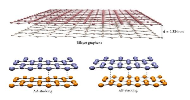
Figure 1: Two of the many possible ways of stacking in bilayer graphene.

Staggered potential is defined as follows:

$$\hat{H}_{stag.}=m\sum_{i=1}^{2}\sum_{X,Y}\Bigl{[}(-1)^{i+1}\delta_{X_{A}Y_{A}}+(-1)^{i}\delta_{X_{B}Y_{B}}\Bigr{]}(\hat{a}_{X_{i}}^{+}\hat{a}_{Y_{i}}+\hat{b}_{X_{i}}^{+}\hat{b}_{Y_{i}}),$$ (5)

where $m$ represents bare mass of fermions and $\delta_{X_{A}Y_{A}}$ ($\delta_{X_{B}Y_{B}}$) means, that the sites $X$ and $Y$ are equal and both belong to sublattice $A$ ($B$). We need this ”staggered” potential for two reasons: firstly, it serves as a primer for the ground state of G-type AFM ordering, for which the formation of energy gap was predicted, and secondly, it regularizes zero modes of the Dirac operator. In the absence of interaction AA-BLG has no energy gap [5], thus the lattice calculations have been performed for a few values of $m$ and than observables were extrapolated to the point $m$ = 0.

Finally, Coulomb part of the Hamiltionian (1) has the form:

$$\hat{H}_{int.}=\frac{1}{2}\sum_{i,j=1}^{2}\sum_{X,Y}\hat{q}_{X_{i}}V_{XY}^{ij}\hat{q}_{Y_{j}},$$ (6)

where $\hat{q}_{X_{i}}=\hat{a}^{+}_{X_{i}}\hat{a}_{X_{i}}-\hat{b}^{+}_{X_{i}}\hat{b}_{X_{i}}$ is the charge operator for the site $X$ on the layer $i$ and $V_{XY}^{ij}$ represents interaction potential between the sites $X_{i}$ and $Y_{j}$ (because the Fermi velocity is approximately $c/315$ in AA-BLG, electron-electron interaction may be considered as instantaneous). The introduced potential $V_{XY}^{ij}$ takes into account the screening by electrons at $\sigma$-orbitals at small distances, it is piecewise-defined: within one layer the values for the on-site interaction potential ($V_{xx}$), the potentials between nearest neighbours ($V_{01}$), next-to-nearest neighbours ($V_{02}$) and next-to-next-to-nearest-neighbours ($V_{03}$) are fixed and taken from [12] (table I, 3d column), while the potential at distances $r>2a$ is considered as Coulomb, starting from $V_{03}$. Potential for the sites, located at different layers, is introduced as usual Coulomb potential. Taking into account the screening effect in lattice model of monolayer graphene and AA-BLG can be crucial point for reproduction of real physics in simulations, because effects of electron-electron interaction are very sensitive to the modification of the short-range potentials [10].

Hereafter we will use the standard formalism of statistical QFT [13][14]. The partition function for the system is defined as follows:

$$Z=Tr\left(e^{-\beta\hat{H}}\right),$$ (7)

where $\beta=1/T$ is the inverse temperature of electron gas. To calculate the partition function we have to perform Suzuki-Trotter decomposition:

$$Tr\left(e^{-\beta\hat{H}}\right)=Tr\left(e^{-\Delta\tau(\hat{H}_{tb}+\hat{H}_{stag.}+\hat{H}_{int.})}\right)^{N_{t}}=$$

$$=Tr\left(e^{-\Delta\tau(\hat{H}_{tb}+\hat{H}_{stag.})}e^{-\Delta\tau\hat{H}_{int.}}e^{-\Delta\tau(\hat{H}_{tb}+\hat{H}_{stag.})}e^{-\Delta\tau\hat{H}_{int.}}\ldots\right)+O(\Delta\tau^{2}),$$ (8)

where $\Delta\tau=\beta/N_{\tau}$, and insert Grassmannian coherent states between the exponentials [13]. The point here is that $\hat{H}_{int.}$ is not the quadratic form of $\hat{a}$ and $\hat{b}$, so it is convenient to decompose $e^{-\Delta\tau\hat{H}_{int.}}$ using the Hubbard-Stratonovich transformation [15]:

$$e^{-\frac{\Delta\tau}{2}\sum\limits_{X,Y}\hat{q}_{X}V_{XY}^{ij}\hat{q}_{Y}}=\int\mathcal{D}\varphi e^{-\frac{1}{2\Delta\tau}\sum\limits_{X,Y}\varphi_{X}V^{-1}_{XY}\varphi_{Y}-i\sum\limits_{X}\varphi_{X}\hat{q}_{X}},$$ (9)

where $\varphi_{X}$ defines real-valued scalar field (Hubbard field) at the site $X$ (layer indices on the r.h.s. of (9) were omitted for notation compactness). After some algebra, we arrive at the following expression for the partition function:

$$Z=\int\mathcal{D}\varphi\textsl{det}(M^{+}M)e^{-S[\varphi]},$$ (10)

where $M$ is the fermionic operator for electrons,

$$S[\varphi]=\frac{1}{2\Delta\tau}\sum_{\tau}\sum_{i,j=1}^{2}\sum_{X,Y}\varphi_{Xi}^{\tau}\left(\hat{V}^{-1}\right)^{ij}_{XY}\varphi_{Yj}^{\tau}$$ (11)

represents Hubbard action, and Hubbard fields in this sum are located only at odd time layers. It is important to note, that due to the decomposition (2) the space-time lattice has $2N_{t}$ time layers, p.b.c. in time direction are introduced for Hubbard fields. Dirac operator $M$ has the following form ($t=0,\ldots,N_{t}-1$, a.p.b.c. in time direction are considered for fermion fields):

$$M_{XiYj}^{\tau^{\prime}\tau}=\delta^{\tau^{\prime},\tau}\delta_{ij}\delta_{XY}-\delta^{\tau^{\prime},2t}(\delta_{ij}\delta_{XY}+\Delta\tau A_{XiYj})\delta^{\tau,2t+1}-\delta^{\tau^{\prime},2t+1}\delta_{ij}\delta_{XY}e^{i\varphi_{Xi}^{2t+2}}\delta^{\tau,2t+2}$$ (12)

where $A^{XiYj}$ is a real matrix and is defined as follows:

$$A_{XiYj}=t\delta_{ij}\left(\delta_{X\in A}\sum_{b=0}^{2}\delta_{Y,X+\rho_{b}}+\delta_{Y\in B}\sum_{b=0}^{2}\delta_{X,Y-\rho_{b}}\right)+t_{0}\delta_{XY}\left(\delta_{i1}\delta_{j2}+\delta_{i2}\delta_{j1}\right)-$$ (13)

$$-m\delta_{ij}\left(\left(-1\right)^{i+1}\delta_{X_{A}Y_{A}}+\left(-1\right)^{i}\delta_{X_{B}Y_{B}}\right).$$

$\rho_{b}$ in (13) denote a set of three vectors, which point from the site of the sublattice $A$ within hexagonal lattice to its nearest neighbours belonging to sublattice $B$.

The formation of the energy gap in the AA-BLG energy spectrum may be examined by the calculation of the AFM condensate:

$$\Delta n=n_{1A\uparrow}-n_{2A\uparrow}=n_{1B\downarrow}-n_{2B\downarrow},$$ (14)

where $n_{i\alpha\uparrow(\downarrow)}$ denotes the number of electrons with spin up (spin down) on the layer $i=1,2$ and sublattice $\alpha=A,B$. Only simultaneous breaking of interlayer and sublattice symmetries may lead to the gap opening [6]. Moreover, the energy gap may be evaluated within the mean field approximation as $\Delta=V_{xx}\Delta n/2$ at small enough $\Delta n$. Thermodynamic expectation variable for (14) has the following form:

$$\left\langle\Delta n\right\rangle=\frac{1}{N_{\tau}N}\sum_{\tau}\left\langle\sum_{X\in A}\Bigl{(}\hat{M}^{-1}_{X2X2}-\hat{M}^{-1}_{X1X1}\Bigr{)}\right\rangle=\frac{1}{N_{\tau}N}\sum_{\tau}\left\langle\sum_{X\in B}\Bigl{(}\hat{M}^{-1}_{X1X1}-\hat{M}^{-1}_{X2X2}\Bigr{)}\right\rangle,$$ (15)

where $N$ represents the number of spatial lattice sites in one sublattice.

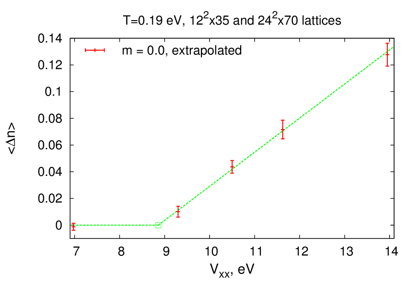
Figure 2: The dependence of the AFM condensate on the on-site interaction potential $V_{xx}$ at fixed temperature. AFM condensate vanishes at the value $V_{xx}^{c}=(8.89\pm 0.33)$ eV.

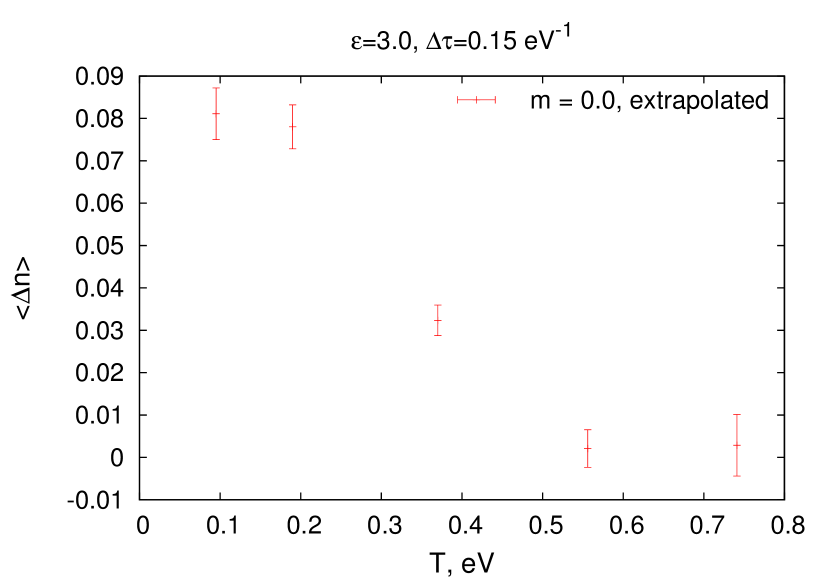
Figure 3: The dependence of the AFM condensate on the temperature. All potentials, except $V_{xx}$, were rescaled by the factor of $\epsilon=3.0$: $V^{ij}_{XY}\rightarrow V^{ij}_{XY}/3.0$.

3 Numerical results and discussion

Simulations were performed on the lattices with spatial size from $12\times 12$ to $24\times 24$ and temporal sizes from $N_{\tau}=9$ to $N_{\tau}=70$, $\Delta\tau=0.15$ eV^-1 (the temperature of electron gas is defined as $T=1/(N_{\tau}\Delta\tau)$, which follows from (2)). The following bare fermion masses were examined for each lattice: $m=0.1$ eV, $0.15$ eV, $0.2$ eV, $0.25$ eV, $0.3$ eV; than the quadratic extrapolation to $m=0.0$ was performed for the calculation of the AFM condensate. We generated 150 — 300 statistically independent configurations for every value of mass, $\Phi$-algorithm was used in simulations.

The first result is presented at Fig. 3 and shows the dependence of AFM condensate (15) on the on-site interaction potential $V_{xx}$ (other potentials are fixed) at particular temperature. This dependence is almost linear and linear extrapolation yields to the critical value $V_{xx}^{c}=(8.89\pm 0.33)$ eV, where $\left\langle\Delta n\right\rangle$ vanishes. On the contrary, mean-field approximation with only on-site Coulomb interaction taken into account predicts nonvanishing exponential dependence for the energy gap [6]. From this one can conclude, that long-range electron-electron interactions work against the formation of the energy gap and produce a noticeable impact on the collective phenomena in the AA-BLG.

The second result is shown at Fig. 3 and represents the dependence of $\left\langle\Delta n\right\rangle$ on temperature for the fixed values of potentials. In these measurements all potentials, except $V_{xx}$, were rescaled by the factor of $\epsilon$: $V^{ij}_{XY}\rightarrow V^{ij}_{XY}/\epsilon$ (inscription ”$\epsilon=3.0$” in the caption over the graph). Thus $\epsilon$ may be considered as a dielectric permittivity of the substrate, on which AA-BLG sample is located. The plateua for $\left\langle\Delta n\right\rangle$ at small temperatures and the transition at $T\approx 0.37$ eV can be clearly seen at the Fig. 3, and $\left\langle\Delta n\right\rangle$ can be considered as an order parameter for the AFM phase transition. At high temperatures $\left\langle\Delta n\right\rangle\approx 0$, what means, that AFM ordering is destroyed by thermal fluctuations.

- [1] A. H. Castro Neto, F. Guinea, N. M. R. Peres, K. S. Novoselov, and A. K. Geim, Rev. Mod. Phys. 81, 109–162 (2009).
- [2] A. V. Rozhkov, G. Giavaras, Y. P. Bliokh, V. Freilikher, and F. Nori, Physics Reports 503, 77–114 (2011).
- [3] M. I. Katsnelson, Graphene: Carbon in Two Dimensions, Cambridge University Press, Cambridge 2012.
- [4] J. Borysiuk, J. Soltys, and J. Piechota, Journal of Applied Physics 109, 093523 (2011).
- [5] E. Prada, P. San-Jose, L. Brey, H. A. Fertig, Solid State Communications 151, 1075–1083 (2011).
- [6] A. L. Rakhmanov, A. V. Rozhkov, A. O. Sboychakov, and F. Nori, Phys. Rev. Lett. 109, 206801 (2012).
- [7] A. O. Sboychakov, A. L. Rakhmanov, A. V. Rozhkov, and F. Nori, Phys. Rev. B 87, 121401 (2013).
- [8] Z. Liu, K. Suenaga, P. J. F. Harris, and S. Iijima, Phys. Rev. Lett. 102, 015501 (2009).
- [9] P. V. Buividovich and M. I. Polikarpov, Phys. Rev. B 86, 245117 (2012)
- [10] M. V. Ulybyshev, P. V. Buividovich, M. I. Katsnelson, and M. I. Polikarpov, Phys. Rev. Lett. 111, 056801 (2013).
- [11] J.-C. Charlier, J.-P. Michenaud, and X. Gonze, Phys. Rev. B 46, 4531–4539 (1992).
- [12] T. O. Wehling, E. Şaşıoğlu, C. Friedrich, A. I. Lichtenstein, M. I. Katsnelson, and S. Blügel, Phys. Rev. Lett. 106, 236805 (2011).
- [13] I. Montvay and G. Münster, Quantum fields on a lattice, Cambridge University Press, Cambridge 1994.
- [14] C. Gattringer and C. B. Lang, Quantum Chromodynamics on the Lattice: An Introductory Presentation, Springer, Berlin Heidelberg 2010.
- [15] R. C. Brower, C. Rebbi, and D. Schaich, in proceedings of Lattice 2011, \posPoS(Lattice 2011)056.