Electronic specific heat of DNA: Effects of backbones and disorder

Abstract

In this present work we report the results of our investigation on the electronic specific heat (ESH) of DNA molecule modelled within the tight-binding framework. We take four different DNA sequences ranging from periodic, quasi-periodic to random and studied both ESH and also the density of states to supplement our ESH results. The role of the backbone structure and the effects of environment on ESH are discussed. We observe that irrespective of the sequences there is a universal response of the ESH spectra for a given disorder. The nature of response of specific heat on backbone disorder is totally opposite in low and high temperature regimes.

I Introduction

Since the last decade, interest in studying the electrical properties of DNA has enhanced considerably as it appears that DNA can conduct electrons, and becomes a promising agent for future nanoelectronic devices which can help to overcome the drawbacks like energy efficiency of present silicon-based devices. Not only this, it has many advantageous properties like self-assemble and self-replication which can make it possible to produce nanostructures with greater precision that is not achievable with classical silicon-based technology winfree . The question whether DNA or in broad aspect biomolecules can conduct electrons or not, was first addressed by Eley and Spivey eley in 1962. The first effort to use organic molecules as electronic components started also quite early in 1974 aviram , but the lack of knowledge of electrical properties of DNA made the task quite difficult. With time, the advent of new-generation sophisticated techniques and low temperature measurement facilities make it possible to investigate the physical properties of DNA and other biomolecules. Till date a large number of studies have been performed on electronic transport properties of DNA. A various number of different techniques have been applied which include measurements on single-stranded DNA braun ; porath , measurements on oriented DNA strands on lipid films okahata , measurement on the current-voltage (I-V) characteristics of unordered DNA on the nanocontacts lee ; otsuka , and also on artificially made poly(GC) chains fink . Despite these vast efforts no conclusive results appear, on contrary DNA behaves in various modes in electrical conduction, such as an insulator storm , wide-band gap semiconductor porath , ohmic fink , and even proximity-induced superconductor at low temperature kasumov . This large variety of experimental results led to various theoretical models in which electrical transport is mediated by polarons conwell , solitons hermon , electrons and holes dekker ; ratner ; beratan . Thus electronic transport properties of DNA still remain quite debatable and Ref. endres ; alburev provide a vivid review.

While there is so much effort to understand the electrical properties of DNA, only mere number of attempts have been made to study its thermal and thermodynamic properties moreira1 ; sarmento ; moreira2 ; moreira3 . Recently a study mendes showed that the knowledge of thermal properties of different biomolecules (e.g., polypeptides etc. ) may become helpful in the determination process of different neurodegenerative diseases like Alzheimer and Parkinson. In our work we would like to extend the knowledge of thermal properties of DNA through study of specific heat in details. Our main aim is to investigate the role of backbones on the electronic specific heat (ESH) spectra, with the purpose of finding the likeness and dis-likeness among them and to predict some kind of standard behavior. We model DNA within the tight-binding framework, incorporating its backbone structure which was lacking in the previous studies moreira1 ; sarmento ; moreira2 ; moreira3 ; mauriz ; albu , to investigate the effects of the presence of backbones and also of the environment. We use four DNA sequences ranging from periodic, quasi-periodic to random, and see that irrespective of sequences the features of specific heat are similar in the clean case (no disorder) and this behaviour prevails even in presence of environmental effects at any particular disorder.

The rest of the paper is organized in the following way: In Sec. 2 we present the tight-binding Hamiltonian and discuss about our theoretical formulation. In Sec. 3 we show our numerical results and finally summarize in Sec. 4.

II Model and Theoretical Formulation

To study the ESH spectra of DNA molecule we use the so-called dangling backbone ladder model (DBLM) klotsa ; gcuni within the tight-binding framework, as it is more realistic than the simple ladder model since the former one incorporates the backbone structure of DNA. As the sugar-phosphate backbones are negatively charged and form the outer part of the double-helix, they can easily interact with environment and the substrates on which experiments are performed and the backbone site energies get changed randomly storm ; kasumov ; barnett ; tran ; zhang ; pablo ; lcai ; sourav . Therefore by introducing disorder in the backbone site-energies we can incorporate environmental effects into the system which quite well replicate the experimental situations.

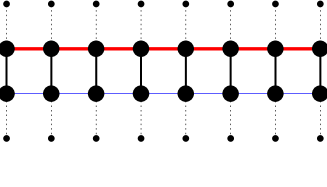
Figure 1: (Color online) Pictorial view of the dangling backbone ladder model to study ESH spectra of double-stranded DNA. The red (thick) and blue (thin) lines are the two strands and the large solid dots on them are the nucleotides. The small black dots on the upper and lower sides of the ladder represent the backbone sites and the dotted lines between the two types of dots represent the coupling between the nucleotides with the corresponding backbone sites.

The effect of environment on the thermal properties of DNA, specially on the specific heat is so far not well-explored, hence for this purpose we use the following tight-binding Hamiltonian of the DBLM to mimic DNA molecule (see Fig. 1)

$$H_{DNA}=H_{ladder}+H_{backbone}~{},$$ (1)

where,

$$H_{ladder} =\sum\limits_{i=1}^{N}\sum\limits_{j=I,II}\left(\epsilon_{ij}c^{\dagger}_{ij}c_{ij}+t_{ij}c^{\dagger}_{ij}c_{i+1j}+\mbox{H.c.}\right)$$ (3)

$$~{}~{}~{}~{}~{}~{}~{}~{}~{}~{}~{}~{}~{}~{}~{}~{}~{}+\sum_{i=1}^{N}v\left(c^{\dagger}_{iI}c_{iII}+\mbox{H.c.}\right)~{},$$

$$H_{backbone} =\sum\limits_{i=1}^{N}\sum\limits_{j=I,II}\left(\epsilon_{i}^{q(j)}c^{\dagger}_{iq(j)}c_{iq(j)}\right.$$

$$~{}~{}~{}~{}~{}~{}~{}~{}~{}~{}~{}~{}~{}~{}~{}~{}~{}+\left.t_{i}^{q(j)}c^{\dagger}_{ij}c_{iq(j)}+\mbox{H.c.}\right)~{},$$

where $c_{ij}^{\dagger}$ and $c_{ij}$ are the electron creation and annihilation operators at the ith nucleotide at the jth stand, $t_{ij}=$ nearest neighbour hopping amplitude between nucleotides along the jth branch of the ladder, $\epsilon_{ij}=$ on-site energy of the nucleotides, $\epsilon_{i}^{q(j)}=$ on-site energy of the backbone site adjacent to ith nucleotide of the jth strand with $q(j)=\uparrow,\downarrow$ representing the upper and lower strands respectively, $t_{i}^{q(j)}=$ hopping amplitude between a nucleotide and the corresponding backbone site, and $v=$ vertical hopping between nucleotides in the two strands of the ladder. For simplicity, we set $\epsilon_{i}^{q(j)}=\epsilon_{b}$, $t_{ij}=t_{i}$ and $t_{i}^{q(j)}=t_{b}$.

To study the electronic specific heat of the DNA molecule, we use the most general formalism where the specific heat at constant volume is given by the partial derivative of average energy of the system with respect to temperature

$$C_{v}=\frac{\partial<E>}{\partial T}$$ (4)

where,

$$<E> =\sum\limits_{i=1}^{N}(E_{i}-\mu)f(E_{i})$$ (5)

$$f(E_{i}) =\frac{1}{1+\exp(\frac{E_{i}-\mu}{k_{B}T})}$$ (6)

where $<E>$ is the average energy of the system, $E_{i}$ the energy of an electron at the ith eigenstate, $\mu$ is the chemical potential, T is the temperature, $k_{B}$ is the Boltzmann constant and $f(E_{i})$ is the occupation probability of the ith eigenstate according to Fermi-Dirac statistics. Using the expressions of $<E>$ and $f(E_{i})$ we find the following expression for electronic specific heat (ESH) of DNA

$$C_{v}=\sum\limits_{i=1}^{N}\frac{(E_{i}-\mu)^{2}\exp(\frac{E_{i}-\mu}{k_{B}T})}{{k_{B}}T^{2}(\exp(\frac{E_{i}-\mu}{k_{B}T})+1)^{2}}$$ (7)

To explain the ESH spectra we also study the electronic density of states (DOS) of the system. We use Green’s function formalism to find DOS of the system which is given by

$$\rho(E)=-\frac{1}{\pi}{\rm Im[Tr[G(E)]]}$$ (8)

where, $G(E)=(E-H+i\eta)^{-1}$ is the Green’s function for the entire DNA molecule with electron energy E as $\eta\rightarrow 0^{+}$, $H=$ Hamiltonian of the DNA, and, ${\rm Im}$ and ${\rm Tr}$ respectively represents imaginary part and trace over the entire Hilbert space.

III Results and Discussions

To study the ESH of DNA, we take four different DNA sequences, of which two are periodic, one is random and another is quasi-periodic. In the present work we take Fibonacci sequence as a prototype example of a quasiperiodic sequence which is derived using the inflation rule : A$\rightarrow$AT, T$\rightarrow$A. In order to investigate the effect of backbone environment, we first study the simple ladder model without any backbone and then the dangling backbone ladder model, which incorporates the backbone structure. In DBLM environmental fluctuations are incorporated introducing disorder into the backbone sites. To represent the actual experimental situation, in this work we simulate the environmental fluctuations including also the effect of water environment by distributing the backbone site-energy $\epsilon_{b}$ randomly within the range $[\bar{\epsilon}_{b}$-w$/2,\bar{\epsilon}_{b}$+w$/2]$, where $\bar{\epsilon}_{b}$ represents the average backbone site energy and w being the disorder strength. To have a physical insight about the ESH of DNA we have also evaluated the DOS of the four DNA sequences as stated earlier for various disorder strengths (w). For numerical calculations the on-site energies of the nucleotides ($\epsilon_{ij}$) are taken as the ionization potential and the following numerical values are used in our work: $\epsilon_{G}$= 8.177 eV, $\epsilon_{C}$= 9.722 eV, $\epsilon_{A}$= 8.631 eV, $\epsilon_{T}$= 9.464 eV. The intrastrand hopping amplitude between identical neighbouring bases is taken as t= 0.35 eV while that between unlike nucleotides is taken as t= 0.17 eV. We take interstrand hopping parameter i.e., vertical hopping to be v= 0.3 eV. The parameters used here are adopted from the first-principle calculations voit ; yan ; senth . The hopping between a nucleotide and corresponding backbone is taken as $t_{b}$= 0.7 eV sourav ; cuni . We also set $k_{B}$=1.

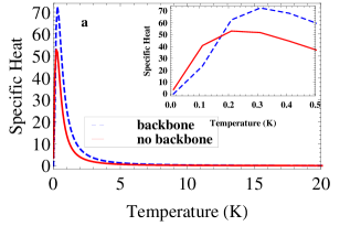
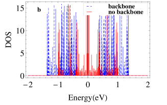
Figure 2: (Color online) a. Electronic specific heat $(C_{v})$ vs temperature ($T$) plot with and without backbone (no sequence, all site-energies are set to zero). $C_{v}$ increases as we introduce backbone into the system except at low temperature (see inset). b. Density of states (DOS) vs. energy (E) with and without backbone. It is clearly visible that due to introduction of backbone a gap opens in the spectrum.

In Fig. 2 we show the behavior of specific heat ($C_{v}$) with temperature ($T$) for a simple ladder model and also for the DBLM which incorporates the backbone structure of the DNA. For the sake of comparisons of both the models we set the site-energies of the nucleotides and the backbone sites to zero. Here we have no sequencing of DNA and also we have ignored disorder ( i.e., w=0) due to environmental fluctuations. It is clear from the figure that due to the presence of backbone, $C_{v}$ gets increased at almost all the temperatures, excepting a small low-temperature region. The corresponding DOS profiles are also shown alongside, which reveals that a gap opens up in presence of backbones.

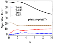
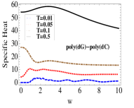
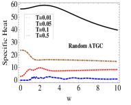
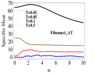
Figure 3: (Color online) Electronic specific heat $(C_{v})$ as a function of backbone disorder strength (w) for four different DNA sequences at low temperature ($T<$2K). $C_{v}$ decreases with disorder (w) except initial rise at low w for all the cases.

First let us explain the basic nature of the $C_{v}$ vs temperature ($T$) curve. At low temperature only the states within the range $E_{F}\pm kT$ are accessible to the electrons, with $E_{F}$ being the Fermi energy. As the average energy of the system is given by $<E>$ = $\int E\rho(E)f(E)dE$, at low temperature we can make the following approximations: dE $\approx$ kT, $\rho(E)\approx\rho$ = a constant, f(E) $\approx$1, and the average energy becomes $<E>~{}\approx\rho k^{2}T^{2}$. Then specific heat becomes $C_{v}$ = $\rho k^{2}T$, being proportional to the temperature, and $C_{v}$ will increases with temperature at low temperature. Let us now see the high temperature behaviour of DNA. The DNA system is a finite one, its energy spectra forms a band of finite width and at high temperature all these states are accessible to the electrons. Now as we increase the temperature, in the very high temperature limit almost all the states are equally populated and the average energy $<E>$ becomes almost independent of temperature. So as we increase temperature from low temperature regime, specific heat initially increases with temperature and then it decreases with temperature and finally goes to zero in the very high temperature regime.

Figure 4: (Color online). Density of states (DOS) profiles for four DNA sequences at different disorder strengths (w). a1-a7 are poly(dA)-poly(dT), b1-b7 are poly(dG)-poly(dC), c1-c7 are random ATGC and d1-d7 are Fibonacci sequences for disorder strength w= 0, 0.5, 2, 5, 10, 15, 20 respectively along vertical lines.

Following similar arguments we can now explain the behavior of the result of Fig. 2. A gap opens up in the middle of the spectrum due to presence of the backbones, and we have a gap at Fermi level in the half filled case. With increase of temperature at the low temperature range initially no states are accessible to the electrons. Now at sufficiently high temperature, when thermal energy becomes comparable to the energy gap of the system, the excited states of the DBLM gradually become accessible to the electrons despite of the energy gap. Thus $<E>$ of the system increases with T at a slower rate than the simple ladder model without backbone since it has no gap in the spectrum. So, initially at the low temperature regime $C_{v}$ gets lowered due to introduction of the backbones (see inset of Fig. 2). As the excited states of DBLM has energy higher than that of the simple ladder model, so $<E>$ will increase at a much higher rate at high temperature and accordingly $C_{v}$ will be higher due to presence of backbones in the high temperature regime.

In Fig. 3 we plot the variation of specific heat with backbone disorder in the low temperature range T$<$2K. It is observed from the figure that $C_{v}$ increases first at low disorder and then it decreases monotonically as the disorder strength increases. The reason is clear from the DOS profiles provided in Fig. 4. At zero disorder (w=0) there is gap in the system for all the sequences, for small w new states started to appear near around the Fermi energy $(E_{F})$ and the gap started to diminish. These new states can be accessed at low temperature, so at low disorder $C_{v}$ increases. For large disorder the gap vanishes, and the band expands beyond the edges, thus new excited states are coming out around the band-edges at the cost of the states around the $E_{F}$ (band-center) as the total number of states is fixed for the system. So, for large w the DOS falls around $E_{F}$, hence apart from a initial rise $C_{v}$ will decrease at low temperature.

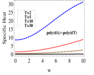
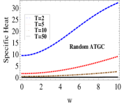
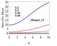
Figure 5: (Color online) Electronic specific heat $(C_{v})$ as a function of backbone disorder strength (w) for four different DNA sequences at high temperature ($T>$2K). $C_{v}$ increases monotonically with disorder (w) for all the cases.

In Fig. 5 we show the variation of $C_{v}$ with backbone disorder strength (w) for the high temperature (T$>$2K) range, and it exhibits that $C_{v}$ increases with temperature. To explain these we once again look at the corresponding DOS profile presented in Fig. 4. At the high temperature all the states are accessible, now as we increase disorder, new states are appearing around the band-edges and the energy of these states also increase with w. As these states has high energy cost, the rate of change of average energy $<E>$ with T also gets increased as we increase w and consequently $C_{v}$ increases with T in the high temperature regime.

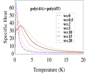
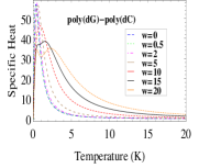
Figure 6: (Color online) Variation of electronic specific heat ($C_{v}$) with temperature ($T$) at different disorder strength (w) for four DNA sequences. Uniform behavior of $C_{v}$ under disorder irrespective of the sequences.

In Fig. 6 we show the variation of $C_{v}$ with temperature (T) for four DNA sequences at various backbone disorder strength (w). In all the plots, at low temperature $C_{v}$ reduces with increasing w while it gets enhanced with w at high temperature as discussed earlier. The peak of the $C_{v}$ vs. T curve, which determines the crossover temperature, also decreases and shifts towards the high temperature as we increase disorder strength. There exists some fluctuations in $C_{v}$ at low temperature under sufficiently high disorder (w$>$5). Earlier this kind of oscillatory behavior of ESH was reported by E. L. Albuquerque et. al. albu at low temperature for the quasi-periodic sequences only, here we get the same kind of fluctuations for all the sequences at low temperature due to environmental effects.

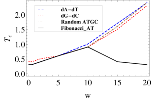
Figure 7: (Color online) Variation of crossover temperature ($T_{c}$) with backbone disorder strength (w). Except the Fibonacci one the nature of variation is almost same for all the sequences.

In Fig. 7 we show the dependence of crossover temperature ($T_{c}$) (i.e., the temperature at which $C_{v}$ becomes maximum) on backbone disorder (w). It shows that $T_{c}$ increases monotonically with w, the rate of increase being not uniform everywhere, for all the DNA sequences excepting the quasi-periodic Fibonacci one. For Fibonacci sequence $T_{c}$ increases upto a certain disorder strength and then it decreases.

IV Concluding Remarks

Till date thermal properties of DNA and other biomolecules are not yet well explored. We make an attempt to examine the electronic specific heat response of DNA by modelling it by the tight-binding Hamiltonian. Though there are some results available in the literature on DNA specific heat moreira1 ; sarmento ; moreira2 ; moreira3 ; mauriz ; albu , but they did not take into account the backbones being a very basic structure of the DNA molecules. In this work we make an attempt to study the effect backbone and also the effect of the environment on the electronic specific heat of DNA. It comes out that the introduction of backbones make drastic changes in the DOS profile, the band structure of the system splits up opening a gap in the central region of the band. Due to the formation of this gap specific heat gets enhanced in presence of backbones over the entire temperature range excepting a narrow low temperature region. On environmental fluctuations, $C_{v}$ exhibits two distinct behaviours, at low temperature it decreases with backbone disorder strength (w) and in the high temperature region it increases with w. We have also seen that the cross-over temperature ($T_{c}$) which corresponds to the maximum of the specific heat vs temperature curve increases with disorder (w). In this way we have been able to put forward a regularized behavior of the ESH of DNA being independent of the sequence we have chosen. The effect of environmental fluctuations on ESH is quite universal both for the clean case (w=0) and also in presence of environmental disorder. It implies that ESH of the system reacts to the environment in the same way irrespective of its sequential variety. In order to verify our predictions experimentally, heat exchange in the process of protein binding, unfolding, ligand association and other bimolecular reactions should be measured with much more reliability. There are three basic techniques used for this measurements, the differential scanning calorimetry (DSC) which measures sample heat capacity with respect to a reference as a function of temperature, isothermal titration calorimetry (ITC) which measures the heat absorbed or rejected during a titration experiment and the third one is thermodynamic calorimetry (for a detail description see Ref. jelesarov ). But unfortunately none of these techniques is able to separate the electronic contribution to the specific heat of biomolecules, as they measure all contributions including the vibrational ones. However, we hope that there will be experimental verification of our results and other investigations to find thermal properties of DNA and alike biomolecules in near future with modifications of the above mentioned tools.

V Appendix

If we take the temperature dependence of chemical potential explicitly into account then the expression of specific heat becomes

$$C_{v}=\frac{1}{4k_{B}T^{2}}[\sum\limits_{i=1}^{N}E_{i}^{2}cosh^{-2}[\frac{(E_{i}-\mu)}{2k_{B}T}]-$$

$$\frac{(\sum\limits_{i=1}^{N}{E_{i}cosh^{-2}[\frac{(E_{i}-\mu)}{2k_{B}T}]})^{2}}{\sum\limits_{i=1}^{N}cosh^{-2}[\frac{(E_{i}-\mu)}{2k_{B}T}]}]$$ (9)

where the chemical potential ($\mu=\mu(n_{e}/N,T)$) can be obtained numerically form the Fermi distribution following

$$n_{e}=\sum\limits_{i=1}^{N}<f(E_{i})>$$ (10)

Here, $n_{e}$ is the number of non-interacting electrons and N is the total number of one-particle accessible states in the system. We check our results using Eq.9, but find no significant changes.

References

- (1) E. Winfree, F. Liu, L. A. Wenzler, and N. C. Seeman, Nature 394, 539 (1998).
- (2) D. D. Eley and D. I. Spivey, Trans. Faraday Soc. 58, 411 (1962).
- (3) A. Aviram and M. A. Ratner, Chem. Phys. Lett. 29, 277 (1974).
- (4) E. Braun, Y. Eichen, U. Sivan, and G. Ben-Yoseph, Nature (London) 391, 775 (1998).
- (5) D. Porath, A. Bezryadin, S. De Vries, and S. Dekker, Nature (London) 403, 635 (2000).
- (6) Y. Okahata, T. Kobayashi, K. Tanaka, and M. Shimomura, J. Am. Chem. Soc. 120, 6165 (1998).
- (7) H.-Y. Lee, H. Tanaka, Y. Otsuka, K.-H. Yoo, J.-O. Lee, and T. Kawai, Appl. Phys. Lett. 80, 1670 (2002).
- (8) Y. Otsuka, H. Lee, J. Gu, J. Lee, K.-H. Yoo, H. Tanaka, H. Tabata, and T. Kawai, Jpn. J. Appl. Phys., Part 1, 41, 891 (2002).
- (9) H. W. Fink and C. Schönenberger, Nature (London) 398, 407 (1999).
- (10) A. J. Storm et al., Appl. Phys. Lett. 79, 3881 (2001).
- (11) A. Y. Kasumov et al., Science 291, 280 (2001).
- (12) E. M. Conwell and S. V. Rakhmanova, Proc. Natl. Acad. Sci. USA 97, 4557 (2000).
- (13) Z. Hermon, S. Caspi, and E. Ben-Jacob, Europhys. Lett. 43, 482 (1998).
- (14) C. Dekker and M. A. Ratner, Physics World 14(8), 29 (2001).
- (15) M. A. Ratner, Nature (London) 397, 480 (1999).
- (16) D. N. Beratan, S. Priyadarshy, and S. M Risser, Chem. Biol. 4, 3 (1997).
- (17) R. G. Endres, D. L. Cox, and R. R. P. Singh, Rev. Mod. Phys. 76, 195 (2004).
- (18) E.L. Albuquerque, U.L. Fulco, V.N. Freire, E.W.S. Caetano, M.L. Lyra, and, F.A.B.F. de Moura, Phys. Rep. 535, 139 (2014).
- (19) D. A. Moreira , E. L. Albuquerque, P. W. Mauriz, and M. S. Vasconcelos, Physica A 371, 441 (2006).
- (20) R. G. Sarmento, G. A. Mendes, E. L. Albuquerque, U. L. Fulco, M. S. Vasconcelos, O. Ujsághy, V. N. Freire, and E. W. S. Caetano, Phys. Lett. A. 376, 2413 (2012).
- (21) D. A. Moreira, E. L. Albuquerque, L. R. da Silva, and D. S. Galvão, Physica A 387, 5477 (2008).
- (22) D. A. Moreira, E. L. Albuquerque, and D. H. A. L. Anselmo Phys. Lett. A. 372, 5233 (2008).
- (23) G. A. Mendes, E. L. Albuquerque, U. L. Fulco, L. M. Bezerril, E. W. S. Caetano, and V. N. Freire, Chem. Phys. Lett. 542, 123 (2012).
- (24) P. W. Mauriz , E. L. Albuquerque, and M. S. Vasconcelos Physica A 294, 403 (2001).
- (25) E. L. Albuquerque, C. G. Bezerra, P. W. Mauriz, and M. S. Vasconcelos Physica A 344, 366 (2004).
- (26) D. Klotsa, R. A. Römer, and M. S. Turner, Biophys. J. 89, 2187 (2005).
- (27) G. Cuniberti, E. Maciá, A. Rodriguez, and R. A. Römer, in Charge Migration in DNA: Perspectives from Physics, Chemistry and Biology, edited by T. Chakraborty, Springer-Verlag, Berlin (2007).
- (28) R. N. Barnett, C. L. Cleveland, U. Landman, E. Boone, S. Kanvah, and G. B. Schuster, J. Phys. Chem. A 107, 3525 (2003).
- (29) P. Tran, B. Alavi, and G. Grüner, Phys. Rev. Lett. 85, 1564 (2000).
- (30) Y. Zhang, R. H. Austin, J. Kraeft, E. C. Cox, and N. P. Ong, Phys. Rev. Lett. 89, 198102 (2002).
- (31) P. J. de Pablo, F. Moreno-Herrero, J. Colchero, J. Gómez Herrero, P. Herrero, A. M. Baró, P. Ordejón, J. M. Soler, and E. Artacho, Phys. Rev. Lett. 85, 4992 (2000).
- (32) L. Cai, H. Tabata, and T. Kawai, Nanotechnology 12, 211 (2001).
- (33) Sourav Kundu and S. N. Karmakar, Phys. Rev. E. 89, 032719 (2014).
- (34) A. A. Voityuk, J. Jortner, M. Bixon, and N. Rösch, J. Chem. Phys. 114, 5614 (2001).
- (35) Y. J. Yan and H. Y. Zhang, J. Theor. Comput. Chem. 1, 225 (2002).
- (36) K. Senthilkumar, F. C. Grozema, C. F. Guerra, F. M. Bickelhaupt, F. D. Lewis, Y. A. Berlin, M. A. Ratner, and L. D. A. Siebbeles, J. Am. Chem. Soc. 127, 14894 (2005).
- (37) G. Cuniberti, L. Craco, D. Porath, and C. Dekker, Phys. Rev. B 65, 241314(R) (2002).
- (38) I. Jelesarov and H. R. Bosshard, J. Mol. Recognit. 12, 3 (1999).