Aggregation of theta-polymers in spherical confinement

Abstract

We investigate the aggregation transition of theta polymers in spherical confinement with multicanonical simulations. This allows for a systematic study of the effect of density on the aggregation transition temperature for up to $24$ monodisperse polymers. Our results for solutions in the dilute regime show that polymers can be considered isolated for all temperatures larger than the aggregation temperature, which is shown to be a function of the density. The resulting competition between single-polymer collapse and aggregation yields the lower temperature bound of the isolated chain approximation. We provide entropic and energetic arguments to describe the density dependence and finite-size effects of the aggregation transition for monodisperse solutions in finite systems. This allows us to estimate the aggregation transition temperature of dilute systems in a spherical cavity, using a few simulations of small, sufficiently dilute polymer systems.

I Introduction

Polymers are often studied as isolated chains. In nature, however, a system of polymers or proteins is usually subject to geometrical confinement, e.g. porous media Dullien1979 or molecular crowding Minton2000 ; Gershenson2010 . This has an effect on structural as well as dynamic properties. Eggers2000 ; Schneider2011 It may also be the reason for entropic forces in segregation processes. Jun2010 ; Jung2012 The process of aggregation itself plays a role in biological systems as well as in technological applications and material design, e.g., in the context of photovoltaic cells. Kim2011

The effect of spherical confinement on the linear extension of polymers in good solvent (modeled by a self-avoiding chain) has been studied by scaling arguments Sakaue2006 , Monte Carlo simulations Cacciuto2006 and Molecular Dynamics simulations Arnold2007 . A relation between the free energy of a single polymer and semi-dilute solutions was established. Adding short-range attraction to the excluded volume leads to a theta polymer that exhibits a collapse transition from an extended coil at large temperatures to a compact globule at lower temperatures. The effect of spherical confinement on a single flexible theta polymer Marenz2012 was shown to be different to (rather stiff) protein Klimov2002 ; Friedel2003 ; Takagi2003 ; Rathore2006 ; Mittal2008 models. For both cases, it was shown that the confinement shifts the location of the collapse transition temperature.

Moreover, spherical confinement provides a safe basis for the study of density effects in finite systems. For a steric confinement, there is at most an effective repulsive interaction. In contrast to periodic boundary conditions it allows to decrease or increase the density systematically without the possibility that the aggregate, or even single polymers, may interact with themselves across the boundaries. The influence of density on the aggregation transition of two lattice proteins has been noticed recently Ni2013 to be similar to that on an ideal gas. In this study we will extend this observation by investigating an off-lattice polymer model that has been successfully applied to peptide JunghansPeptide and polymer aggregation JunghansPolymer ; Zierenberg2014 before. Focusing on the case of flexible homopolymers, we will provide entropic arguments for the density dependence and energetic arguments for finite-size effects which leads to a reasonable description of the density dependence in a spherical confinement. Among others, we demonstrate the competition between single-chain collapse and multi-chain aggregation in the dilute regime, showing the dominance of aggregation and the consequences on structural properties of a single polymer.

The paper is organized as follows: In Sec. II, we briefly describe the employed aggregation model together with the multicanonical method. We mention the applied optimizations and relevant parameters. Section III contains all main results including a discussion of the canonical picture, entropic arguments in the microcanonical picture, and a description of finite-size effects. We finish with our conclusions on the effect of density on the aggregation transition temperature in spherically confined finite polymer systems in Sec. IV.

II Model and Method

We consider a set of $M$ bead-spring polymers confined in a spherical cavity of radius $R_{S}$. Each homopolymer consists of $N$ equal monomers aligned linearly with a finitely extensible nonlinear elastic (FENE) potential between bonded monomers and Lennard-Jones interaction between non-bonded monomers. The interactions are parameterized as in Refs. Binder2001, ; Schnabel2009, ; Zierenberg2014, , namely the FENE potential

$$V_{\rm FENE}(r)=-\frac{K}{2}R^{2}\ln\left(1-[(r-r_{0})/R]^{2}\right),$$ (1)

with $r_{0}=0.7$, $R=0.3$, and $K=40$, as well as the 12-6 Lennard-Jones potential

$$V_{\rm LJ}(r)=4\epsilon\left[(\sigma/r)^{12}-(\sigma/r)^{6}\right],$$ (2)

with $\epsilon=1$ and $\sigma=r_{0}/2^{1/6}$. For numerical reasons and in order to be consistent with the aforementioned literature, the Lennard-Jones potential is cutoff at $r_{c}=2.5\sigma$ such that

$$V^{*}_{\rm LJ}(r)=\begin{cases}V_{\rm LJ}(r)-V_{\rm LJ}(r_{c})&r<r_{c}\\ 0&\mathrm{else}\end{cases}$$ (3)

has the same qualitative behavior and is still continuous at $r_{c}$. The Lennard-Jones potential accounts for excluded volume and short-range attraction such that each polymer can undergo a collapse transition. There is no distinction between the interaction of monomers within the same polymer or between different polymers. In general, we focus in this study on flexible polymers with one exception, when we discuss the direct influence of the density on a specific example of stiff polymers. Stiffness is introduced as a penalty from the discretized polymer curvature. This results in a bending potential

$$V_{\rm bend}(\theta)=\kappa\left(1-\cos\theta\right),$$ (4)

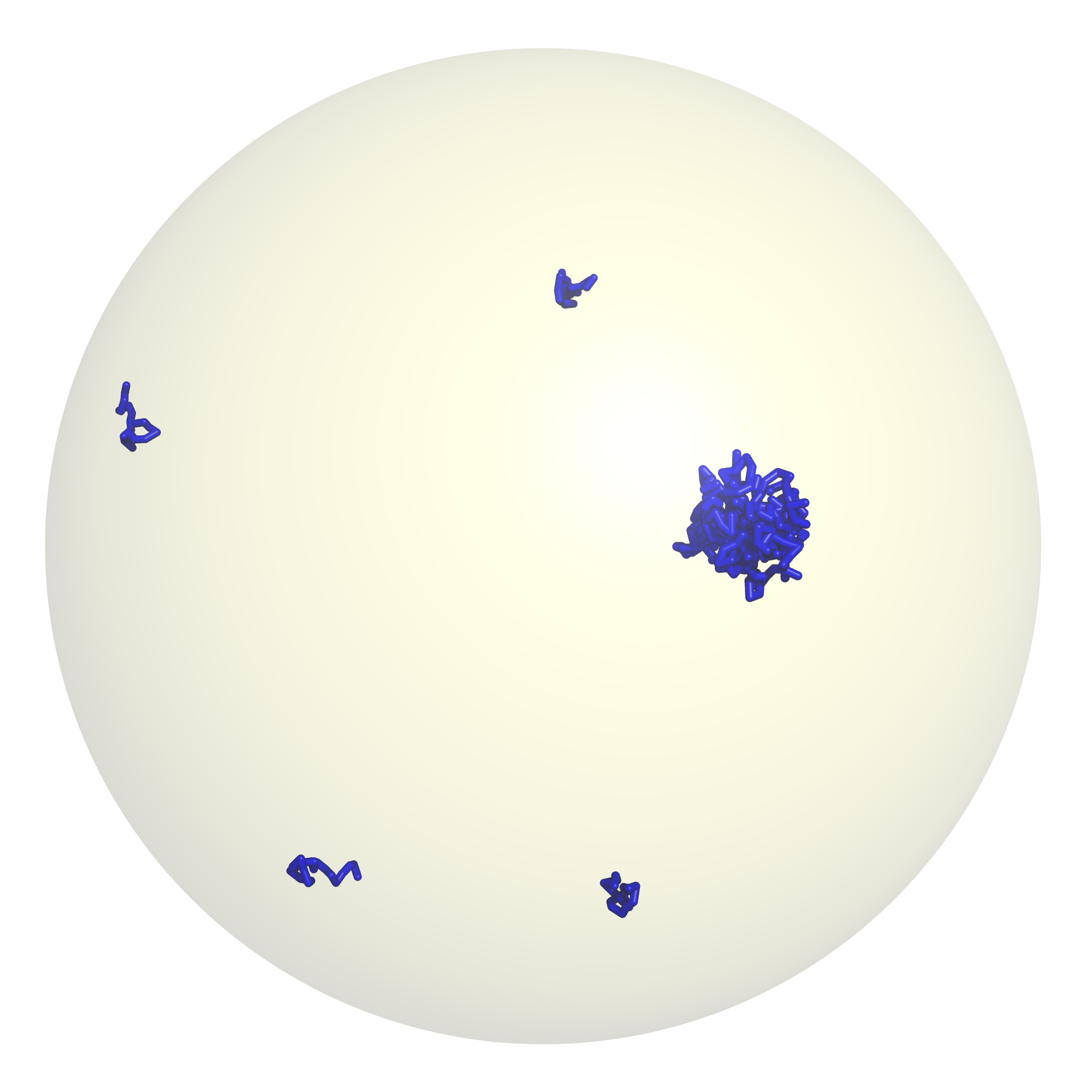
where $\theta$ is the angle between consecutive bond vectors. The polymer system is constraint in a steric sphere such that conformations exceeding the spherical confinement are forbidden, for a snapshot see Fig. 1. In general the radius of the sphere is much larger than the linear extension of a single polymer, which can be estimated within a self-avoiding walk picture to have a radius of gyration $R_{\rm gyr}\propto N^{\nu}$ ($\nu\approx 0.588$). Clisby2010

Figure 1: Snapshot of a polymer system with $M=20$ polymers of length $N=20$ in a sphere with radius $R_{S}=30$. The snapshot was taken in the final production run of the multicanonical simulation and the conformation corresponds to an intermediate state inside the aggregation transition.

We employ Markov chain Monte Carlo simulations in the multicanonical ensemble MUCA ; Janke1998 because aggregation shows characteristics of a first-order phase transition for which this method was proven to be particularly efficient. The method allows to sample a broad temperature range by replacing the Boltzmann weight by an a priori unknown weight function that is iteratively adjusted in order to yield a flat histogram. JankeHist To this end, we first set an energy range obtained from exemplary parallel tempering simulations of small systems. The weight function $W(E)$ is defined on a discretized energy space with 1000 bins in the selected range. Between consecutive iterations the weight function is updated by dividing each entry by the amount of sampled data within the energy bin stored in a corresponding histogram. In order to achieve sufficient statistics for large systems with either a large number of total monomers or a large sphere, we employ parallel multicanonical simulations with up to 256 cores. Zierenberg2013 This parallelization efficiently distributes the required amount of statistics for the weight iteration and speeds up the final data production linearly.

Updates of the system are randomly drawn from a set of moves including single-bead displacement, bond rotation, polymer translation as well as inter- and intra-polymer rearrangement (double-bridging) moves. In order to increase efficiency of the multicanonical method covering a broad energy range, we employ energy-dependent update ranges. These are implemented such that detailed balance is fulfilled. Schnabel2011Adv Increasing the radius of the confining sphere leads to a fast increase of conformational entropy. Thus, the maximal translation step is coupled to the radius of the spherical confinement in order to move polymers across larger distances when the system becomes more dilute. In order to cope with the immense entropy gain properly, we also coupled the number of sweeps per iteration and measurement linearly to the radius of the sphere.

The data from the final equilibrium production run is afterwards reweighted to yield canonical statistics in the desired temperature range $T\in[0.6,3.0]$ where we apply time-series reweighting ($\Delta T=0.1$ steps) including error analysis and histogram reweighting ($\Delta T=0.005$ steps) for the connecting lines in the canonical plots. Reweighting The aggregation transition temperature is calculated by computing the second derivative of the total energy and locating the zero crossing with an iterative time-series reweighting. Errors are obtained from repeating this procedure in the framework of jackknife error analysis. To this end, we combine all but one of the (up to 256) independent time series, calculating a set of highly correlated estimators of the transition temperature. The jackknife error analysis now takes this trivial correlation into account and provides an unbiased error estimate. This is of advantage because the heat capacity is known to yield biased estimators, which we may encounter for small data subsets.

III Results

III.1 Canonical picture

Figure 2: Normalized energy (top) and specific heat (bottom) for $M=8$ flexible polymers of length $N=13$ in spherical confinement. With increasing radius $R_{S}$, the density decreases and the aggregation transition shifts to lower temperatures. Notice, that the principle behavior at large temperature resembles the single polymer (dilute limit) behavior and that the dependence of the amorphous aggregate, at low temperature, follows the characteristics at larger density.

Figure 3: Average end-to-end distance per polymer (top) and its temperature derivative (bottom) for $M=8$ flexible polymers of length $N=13$ in spherical confinement of size $R_{S}$.

Homogeneous aggregation describes the crossover from a separated phase of individual polymers to an aggregated phase in which a fraction of polymers will be condensed into a single macroscopic object. In a strict sense, the notion of phases only applies to infinite systems, whereas polymer systems are argued to be finite because the length of a polymer is finite by nature. However, we adapt the notion of phases to the limit of infinitely many polymers, $M\rightarrow\infty$, at fixed polymer density $\rho=M/V$ and fixed polymer length $N$, where $V=\frac{4\pi}{3}R_{S}^{3}$ is the volume of the confining sphere. Then the notion of phases can be regained in the usual way. In this case, we consider the polymer length to be a system property just like the interaction parameters. It may be expected that above the aggregation transition the polymers will behave as in the dilute limit, exploring the conformational space independently. Fixing the number of polymers and increasing the radius of the confining sphere reduces the density and eventually leads to the dilute limit of isolated polymer chains for $R_{S}\rightarrow\infty$. In order to compare to the dilute limit, we consider the system energy normalized to a single polymer $E/M$ together with its thermal derivative, the specific heat per polymer $C_{V}/M=\beta^{2}\left(\langle E^{2}\rangle-\langle E\rangle^{2}\right)/M$, where $\beta=1/T$ (in units where $k_{B}=1$). In addition, we measure the average end-to-end distance per polymer as the sum over distances between the first and the last monomers each: $\overline{R}_{\rm EE}=\frac{1}{M}\sum_{i=1}^{M}R_{\mathrm{EE},i}$, where $R_{\mathrm{EE},i}$ is the end-to-end distance of a single polymer. For all observables, $\langle...\rangle$ denotes the thermal average.

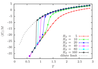
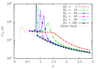
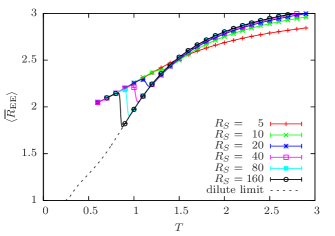
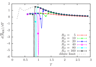
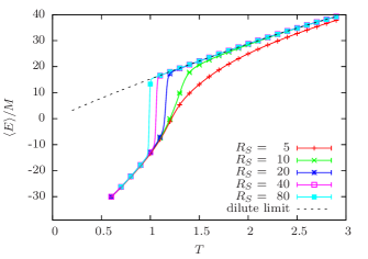
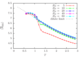
Figures 2 and 3 show the average energy and average end-to-end distance with their thermal derivatives for 8 flexible polymers of length $N=13$ for various sizes of spherical confinement. The lines are results from reweighting the raw data of the final multicanonical production run. We present data points with error bars from an extensive jackknife error analysis Efron1982 at equidistant temperatures only. The curve labeled “dilute limit” is obtained from a separate multicanonical simulation of a single polymer. Note that above the aggregation transition down to the point of structural rearrangement into a single macroscopic object, the polymers follow on average the behavior of the isolated chain of length $N=13$ (dilute limit). This is only hindered for small spheres, in this example $R_{S}=5$, where the separated phase cannot be achieved because the cavity is of the order of the aggregate. This can be understood in terms of the overlap threshold $\Phi^{*}$ of polymer solutions: deGennes If the volume fraction $\Phi=NM\left(\frac{r_{0}}{2}\right)^{3}/R_{S}^{3}$ of a multi-polymer system is much smaller than the intrinsic volume fraction of a single random coil,

$$\Phi^{*}\simeq\frac{N\left(\frac{r_{0}}{2}\right)^{3}}{R_{\rm EE}^{3}}\simeq N^{1-3\nu}\approx N^{-0.76},$$ (5)

where $R_{\rm EE}\simeq r_{0}N^{\nu}$ is the end-to-end distance of a self-avoiding walk with $\nu\approx 0.588$, each polymer may be considered independent and the system is dilute. A volume fraction of the order of this single Gaussian-coil threshold, however, describes the onset of the semi-dilute region. Thus, we look for the point where $\Phi=\Phi^{*}$. Solving this for the radius $R_{S}$ of the spherical confinement, one sees that multi-polymer solutions may be considered dilute for radii sufficiently larger than

$$R_{S}^{c}\simeq r_{0}M^{1/3}N^{\nu}.$$ (6)

The crossover to the semi-dilute regime occurs around $R_{S}\approx R_{S}^{c}$. For $N=13$, $R_{S}^{c}\approx 6.3$ which is consistent with the deviations we observe for $R_{S}=5$ and to a lesser extent also for $R_{S}=10$. Below the aggregation transition in the dilute regime, the canonical observables coincide again because then the spherical confinement has almost no effect on the structural properties of the aggregate.

This implies that the individual flexible polymers each follow the collapse transition of the dilute limit down to the temperature where aggregation suddenly sets in and becomes the major physical process determining the system’s equilibrium properties. For systems with equal inter- and intra-polymer interactions, it has been noticed that collapse and aggregation are not separate processes but that aggregation dominates. JunghansPolymer This is best seen in Fig. 3 where the derivative of the average end-to-end distance shows a broad peak around $T\sim 0.9$ corresponding to the collapse of a single polymer (dilute limit). Sufficiently dilute systems follow this behavior down to the point of aggregation. At first sight surprising is the increase of the average end-to-end distance $\overline{R}_{\rm EE}$ at the aggregation transition (Fig. 3 top). It can be argued that within the aggregate the average end-to-end distance is larger than for the single collapsed polymer because the amorphous aggregates are highly entangled, forming a macroscopic spherical object rather than patching collapsed polymers together. The dominance of the aggregation transition can be understood by its discontinuous nature opposed to the continuous collapse transition. This discontinuous nature follows from a strong structural variation and can be seen as a sharp jump of, e.g., the end-to-end distance. The size of the change increases with decreasing density, see Figs. 2 and 3. Moreover, at sufficiently small densities the polymers are expected to aggregate at those temperatures where single polymers assume globule conformations. However, the energetic arguments in Ref. JunghansPolymer, and the presented data suggest that even then the collapsed conformations should unfold in order to form entangled aggregates as equilibrium conformation.

Figure 4: Normalized energy (top) and average end-to-end distance per polymer (bottom) for $M=8$ rather stiff polymers ($\kappa=9$) of length $N=13$ in a sphere of radius $R_{S}$.

The same observation of coinciding dilute and aggregated phases may be made for rather stiff polymers. For eight polymers of length $N=13$ it was shown Zierenberg2014 that a bending stiffness with $\kappa=9$ leads to polymer bundles in the aggregated phase. In this regime, the dilute limit of a single polymer does not show a collapse transition, on the contrary the individual polymers are driven to elongate in order to minimize curvature, see Fig. 4. As in the case of flexible polymers, the aggregation transition occurs only in a very narrow temperature range and changes the average behavior from that of individual polymers to dense polymers which in this case form polymer bundles. Interesting is that the formation of polymer bundles in the sampled density range leads to an initial increase in the average elongation right below the transition. However, a further reduction of the temperature causes the system to form twisted bundles in which the average end-to-end distance gets reduced again. Zierenberg2014 It may be expected that at even lower densities and consequently lower aggregation temperatures the bundle formation may directly lead to twisted bundles.

As mentioned before, the equilibrium aggregation transition of homopolymers leads to a single macroscopic aggregate instead of multiple smaller aggregates. This can be observed in the total radius of gyration (see Fig. 7 with a detailed discussion in Sec. III.3) which drops to the scale of a single polymer of length $NM$. Despite the non-vanishing probability to form metastable states with several aggregates, these conformations seem to not affect the equilibrium properties significantly away from the transition point.

III.2 Microcanonical picture

The spherical confinement provides a safe and controllable base to study the effect of density on the aggregation transition. In principle, a periodic box would also allow to study this effect. However, the possibility that the aggregate may interact with itself across the boundaries introduces systematic errors, which are hard to tackle as the probability of self-interactions rises with increasing density. This effect gets excluded with the spherical confinement, while introducing at most an effective repulsion from the steric wall.

Here, we consider the number of monomers per polymer $N$ to be a system property that describes the extension of a polymeric object. This is a valid assumption in the dilute limit and in the limit of many polymers, where we focus on the former. In order to show the generality of our results, we consider parameters $N=\{13,20,27\}$ which will show the same qualitative behavior. A more detailed discussion of the influence of $N$ will be given in Sec. III.3.

In order to quantify the effect of density on the aggregation transition, we consider the microcanonical ensemble and start out with the Gibbs construction. The microcanonical entropy is given by the logarithm of the total number $\Omega$ of configurations with a given energy: $S(E)=\ln\Omega(E)$. Moreover, the microcanonical inverse temperature is defined as the local slope of this microcanonical entropy, or in different words its derivative with respect to $E$. Expecting a phase coexistence, there should exist an inverse temperature as local slope to two energy states, equivalent to considering an energy distribution with two peaks in the canonical ensemble. This allows us to estimate the inverse aggregation temperature as the slope of the hull connecting the microcanonical entropy of the aggregated and the separated phase. JankeMicro ; JunghansPeptide ; JunghansPolymer Hence,

$$\beta_{\rm agg}=\frac{S(E_{\rm sep})-S(E_{\rm agg})}{\Delta E}.$$ (7)

Figure 5: The microcanonical entropy $S$ (up to an additive constant) as the logarithmic density of states $\ln\hat{\Omega}$ for $M=8$ polymers ($N=13$), obtained from a microcanonical analysis of the multicanonical data.

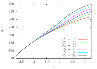
Now, consider a spherical confinement of radius $R_{S}$. Figure 5 shows the microcanonical entropy for $8$ polymers of length $N=13$ obtained as the logarithm of the estimated density of states $\hat{\Omega}(E)$. An estimate of the density of states comes directly from the multicanonical method within the selected energy range when dividing the final histogram by the weight function $\hat{\Omega}(E)=H(E)/W(E)$. The number of states in the aggregated phase will barely be influenced by the confinement, compared to the ensemble of polymers in the fluctuating phase that behaves more like a gas. Therefore, we assume for the separated phase that the number of states will be proportional to $V^{M}$ as in the case of an ideal gas,

$$S(E_{\rm sep})\sim\ln\left[\left(\frac{4\pi}{3}R_{S}^{3}\right)^{M}\right]\propto M\ln R_{S},$$ (8)

thus dominating over $S(E_{\rm agg})$. Assuming that the latent heat will be almost constant with respect to $R_{S}$ for fixed $(M,N)$, we may write $\Delta E=M\Delta e$. This leads to an aggregation temperature depending on the logarithm of the radius of the confining sphere:

$$\beta_{\rm agg}(R_{S})\sim\frac{S(E_{\rm sep})}{\Delta E}\sim\ln R_{S}+\mathrm{const}.$$ (9)

This may be rewritten in terms of the density $\rho$ as well $\beta_{\rm agg}=a_{1}\ln\rho+a_{2}$, which has been observed recently, e.g., for two lattice proteins Ni2013 and polymer adsorption moeddel2010 .

Figure 6: Scaling of the inverse aggregation temperature with the logarithm of the system size for $N=13$. For more detail see Table 1.

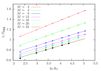
Tables 1, 2, and 3 present aggregation transition temperatures, obtained from the peak location of the specific heat $C_{V}/M$, for a wide range of polymer sizes $N=\{13,20,27\}$ and polymer numbers $M=\{2,4,8,12,16,20,24\}$ as far as possible. Figure 6 shows the inverse aggregation temperature as a function of $\ln R_{S}$ for the example $N=13$. It can be seen that the expected scaling (9) is clearly confirmed by the data and that with increasing $M$ the slopes of the fit become more similar.

Table 1: Aggregation temperatures obtained from the peak location of the specific heat for $N=13$ and $R_{S}\geq 20$. In addition, we present the fit results from $\beta=a\ln R_{S}+b$ for $R_{S}\geq 30$.

$M$		$R_{S}$		$T_{\rm agg}$	fit parameters
2		20		0.8390(6)
2		30		0.7884(6)
2		40		0.7569(5)
2		60		0.7161(14)	0.1831(12) $\ln R_{S}$ + 0.646(5)
2		80		0.6903(6)
2		120		0.6572(11)
2		160		0.6367(18)
4		20		0.9967(12)
4		30		0.9337(4)
4		40		0.8944(4)
4		60		0.8462(9)	0.1588(9) $\ln R_{S}$ + 0.531(4)
4		80		0.8151(7)
4		120		0.7769(20)
4		160		0.752(4)
8		20		1.1399(4)
8		30		1.06385(26)
8		40		1.0179(4)
8		60		0.9601(6)	0.14063(23) $\ln R_{S}$ + 0.4628(10)
8		80		0.92494(22)
8		120		0.8807(9)
8		160		0.85221(27)
12		20		1.2184(4)
12		30		1.1338(5)
12		40		1.0832(7)
12		60		1.0216(7)	0.1367(6) $\ln R_{S}$ + 0.4177(20)
12		80		0.9834(5)
12		120		0.926(4)
12		160		0.9044(13)
16		20		1.2717(5)
16		30		1.1813(5)
16		40		1.1278(6)
16		60		1.0626(7)	0.1363(8) $\ln R_{S}$ + 0.3830(27)
16		80		1.0244(13)
16		120		0.9611(18)
20		20		1.3126(11)
20		30		1.21752(26)
20		40		1.1611(4)
20		60		1.0929(8)	0.1315(5) $\ln R_{S}$ + 0.3748(15)
20		80		1.0504(9)
20		120		0.9998(7)
24		20		1.3451(8)
24		30		1.2459(8)
24		40		1.1873(8)	0.1306(8) $\ln R_{S}$ + 0.3592(29)
24		60		1.1177(6)
24		80		1.0752(9)

Table 2: Same as Table 1 for $N=20$

$M$		$R_{S}$		$T_{\rm agg}$	fit parameters
2		20		1.0373(10)
2		30		0.9793(7)
2		40		0.9430(15)
2		60		0.8944(10)	0.1371(11) $\ln R_{S}$ + 0.555(4)
2		80		0.8649(11)
2		120		0.8266(12)
2		160		0.801(4)
4		20		1.2034(10)
4		30		1.1331(10)
4		40		1.0884(10)
4		60		1.0342(6)	0.1200(10) $\ln R_{S}$ + 0.475(4)
4		80		0.9995(9)
4		120		0.9549(23)
8		20		1.3513(7)
8		30		1.2685(5)
8		40		1.2179(12)
8		60		1.1547(18)	0.1083(4) $\ln R_{S}$ + 0.4202(15)
8		80		1.1156(11)
8		120		1.0659(6)
12		20		1.4331(6)
12		30		1.3408(10)
12		40		1.2861(7)
12		60		1.2185(27)	0.1037(6) $\ln R_{S}$ + 0.3943(22)
12		80		1.1772(16)
12		120		1.1163(19)
12		160		1.0894(12)
16		20		1.4876(4)
16		30		1.3903(7)
16		40		1.3319(5)	0.1058(6) $\ln R_{S}$ + 0.3602(21)
16		60		1.2601(5)
16		80		1.2182(11)
20		20		1.5296(7)
20		30		1.4267(5)
20		40		1.3661(7)	0.1034(5) $\ln R_{S}$ + 0.3495(17)
20		60		1.2928(10)
20		80		1.2466(6)

Table 3: Same as Table 1 for $N=27$

$M$		$R_{S}$		$T_{\rm agg}$	fit parameters
2		20		1.1786(15)
2		30		1.1172(21)
2		40		1.0785(13)
2		60		1.0276(12)	0.1114(10) $\ln R_{S}$ + 0.517(5)
2		80		0.9942(14)
2		120		0.9524(9)
2		160		0.9249(13)
4		20		1.3489(7)
4		30		1.2745(14)
4		40		1.2279(18)
4		60		1.1701(16)	0.0985(10) $\ln R_{S}$ + 0.450(4)
4		80		1.1343(12)
4		120		1.084(4)
4		160		1.0547(28)
8		20		1.4981(10)
8		30		1.4115(8)
8		40		1.3574(9)	0.0925(7) $\ln R_{S}$ + 0.3945(24)
8		60		1.2935(10)
8		80		1.2515(10)
12		20		1.5783(16)
12		30		1.4847(9)
12		40		1.4268(10)	0.0897(6) $\ln R_{S}$ + 0.3691(20)
12		60		1.3564(19)
12		80		1.3128(7)
16		20		1.6338(7)
16		30		1.5332(6)
16		40		1.47264(28)	0.0907(8) $\ln R_{S}$ + 0.3444(27)
16		80		1.3533(16)

III.3 Finite-size effects at polymer aggregation

The effect of stiffness on aggregation of a few polymers in bulk has been investigated recently. Zierenberg2014 It was shown that the polymers form amorphous aggregates in the case of flexible polymers and correlated polymer bundles in the stiff polymer limit. Here, we focus on the flexible limit, where the amorphous aggregate may be argued to behave similarly to a single polymer of length $NM$. Moreover, in this limit it should result in a spherical aggregate with radius $R\sim\left(NM\right)^{1/3}$ as predicted for the collapsed isolated polymer. This should be observable in the total squared radius of gyration

$$R_{\rm gyr}^{2}=\frac{1}{NM}\sum\left(\boldsymbol{r}_{i}-\boldsymbol{r}_{\rm cm}\right)^{2},$$ (10)

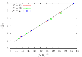
where $\boldsymbol{r}_{\rm cm}$ is the center of mass vector of the total system. For small spheres ($R_{S}=30$) the polymers form stable aggregates at sufficiently high temperatures. Furthermore, the canonical results demonstrate that the amorphous aggregates behave consistently, despite different radii. Figure 7 shows the squared radius of gyration $R_{\rm gyr}^{2}$ of the total system versus the expected scaling function of the total number of monomers $f(NM)=(NM)^{2/3}$. Because our focus is to sample the aggregation transition temperature, we consider a reduced energy range going to sufficiently small energies. However, this does not allow to extrapolate to temperatures far below the aggregation transition temperature. In order to compare the scaling of the squared radius of gyration, we need a fixed temperature that is below the aggregation transition temperature but which is still within the sampled range of our simulations. Both boundaries vary with the length and number of polymers. This leads to a relatively small sample size in Fig. 7 because $T=0.7$ is so large that the smallest systems are not yet in the aggregated state but too small for the large systems to be sampled with the chosen energy range. Nonetheless, it shows the qualitative data collapse that we expected for finite polymer systems.

Figure 7: Data collapse of the squared radius of gyration as a function of $(NM)^{2/3}$. The polymer systems are in spheres of size $R_{S}=30$ with $N=\{13,20,24\}$ at $T=0.7$.

In general, the idea of finite-size scaling is to use small systems in order to make predictions about a system of infinite size and to describe how certain physical properties are approached with increasing system size. In spin systems for example, one may consider the deviation of the transition temperature between the ordered and disordered phases from the value of the infinite system $L\rightarrow\infty$. For polymer aggregation, however, this limit becomes nontrivial. Single polymer studies for example consider finite-size scaling for $N\rightarrow\infty$. In systems with more than one polymer, we have to introduce some sort of boundary conditions and define a density. For the limit of infinitely long polymers, we were not able to think of a density with a well-defined scaling behavior, not changing local system properties.

Thus, we fix $N$ (considering three realizations) and investigate deviations for different $M,R_{S}$ at polymer density $\rho=M/V$ constant. This choice does not change the average local system in the infinite system limit $M\rightarrow\infty$. Although our system sizes are rather small for a quantitatively accurate finite-size scaling, we attempt to draw conclusions about the finite-size effects in small systems.

For systems with a small number of polymers, it is a reasonable assumption that the aggregation transition separates a gas-like phase (see arguments in Sec. III.2) from a homogeneous aggregate and approximate void space. For a larger number of polymers in the dilute regime, there are good arguments for a mixed phase of a macroscopic aggregate and a polymer gas phase in analogy to particle condensation. Nussbaumer2008 ; Zierenberg2014JPCS From our experience with particle systems, we expect to observe even for moderately large system sizes a large fraction of polymers going into the equilibrium aggregate. In any case, the finite aggregate forms a surface such that the system may be compared to “single-domain” non-periodic boundary conditions. The finite-size corrections then are of the order $1/L$, where $L$ is the characteristic system length (for details see also Refs. Privman1990, ; Borgs1995, ). This may be interpreted as competing contributions from the system volume ($\sim L^{d}$) and system surface ($\sim L^{d-1}$). We make use of this observation and consider the linear extension of the aggregate $R_{\rm gyr}$ as characteristic length scale of the system. As we showed in Fig. 7, for flexible polymers the aggregates are spherical and for small systems they include a large fraction of the polymers such that $R_{\rm gyr}\sim M^{1/3}$, where we omitted $N$ which is considered as a fixed system parameter. Thus, our ansatz for monodisperse polymers is

$$T_{\rm agg}(M,\rho)\propto\left(1+s(\rho)M^{-1/3}+\mathcal{O}\left(M^{-2/3}\right)\right),$$ (11)

where $s(\rho)$ determines the size of the leading correction and may depend on the density.

Figure 8: Fit of the finite-size effects for all $N$ at fixed density $\rho=10^{-3}$. Error bars are obtained by error propagation and neglect possible systematic deviations due to higher-order corrections.

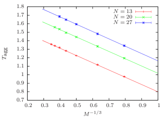
An example of the ansatz is shown in Fig. 8 for the selected $N$ at fixed density $\rho=10^{-3}$. We fitted the data in Tables 1-3 to the dependence (9) and used those fits to interpolate the inverse transition temperature to various dilute polymer densities. Fitting the ansatz for the finite-size effects we obtained the same qualitative results for different densities. As expected, the extrapolated limit would again be depending on $\ln\rho$ (not shown here) and moreover would most probably not be in the infinite system limit. The fit parameter $s$ only slightly depends on the density. Thus, we assume $s$ for the remaining part of the study to be constant. As we mentioned before, we consider $N$ as a system parameter and thus it is not surprising that $s$ is $N$-dependent.

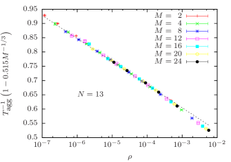
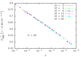
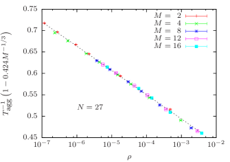
We can combine the finite-size effects in order to rescale the inverse aggregation temperature by multiplying it with the ansatz (11). Considering the polymer density $\rho$ as the relevant parameter, we would then expect that the data falls on a coinciding linear relation. Figure 9 shows a reasonable data collapse for all simulated polymer lengths, where we assumed $s$ constant with its value denoted on the $y$-axes of the plots. The data collapses on a single line is consistent with the developed density dependence and finite-size effects. Despite the $N$-dependent scaling form, this shows that the entropic arguments for the density dependence together with the energetic arguments for the finite-size effects are consistent and allow a reasonably well description of the aggregation transition of a few dilute monodisperse polymers in a spherical cavity.

Figure 9: Rescaled inverse aggregation temperature versus density $\rho$ for all three polymer lengths $N=\{13,20,27\}$. The finite-size correction $s$ in Eq. (11) was assumed to be constant. For $N=13$ one may compare to Fig. 6.

IV Conclusions

Throughout our systematic investigation, we have demonstrated that the separated phase of flexible and stiff polymers corresponds to the dilute limit for sufficiently small densities. The aggregated phase itself is barely influenced by the confinement. In the case of flexible polymers the aggregate may be described as a spherical object, whose size scales like the collapsed state of a single flexible polymer with the same total number of monomers. The spherical confinement effects the location of the aggregation transition of dilute polymers. For denser systems, the separated phase may be suppressed completely; increasing the density even further the aggregate itself will be compressed by the confinement, probably driving the system into its frozen state.

For the case of dilute polymers, we have presented entropic (Sec. III.2), geometric and energetic arguments (Sec. III.3) that allow a description of the rescaled aggregation temperature as a function of density for monodisperse flexible theta polymers. The entropic considerations suggest a linear dependence of the inverse aggregation temperature on the logarithm of the density. We deduced a description of finite-size effects (11) that characterizes the deviations among small systems reasonably well. The system sizes we investigated are most likely too small to capture the behavior of infinite systems. However, for experiments investigating small polymeric systems in confined geometries on the nanoscale, these finite-size effects should be apparent.

The results presented are potentially relevant for experiments with dilute polymer solutions, which investigate single polymer behavior. We showed that even in the case of dilute solutions there exists an aggregation transition that may be estimated by considering a few polymers in sufficiently dilute systems and extrapolating to the dilute limit. In experiments, depending on the actual free-energy barrier and the corresponding relaxation times, it would probably be difficult to observe homogenous aggregation. In principle, estimates of this barrier should be accessible to computer simulations using a proper finite-size scaling ansatz together with sufficiently large system sizes. Our results suggest that this may be done for rather dense systems, which would allow to reach appropriate system sizes – but that remains still to be done in a forthcoming study.