Degradation-based residual life prediction under different environments

Abstract

Degradation modeling has traditionally relied on historical signals to estimate the behavior of the underlying degradation process. Many models assume that these historical signals are acquired under the same environmental conditions and can be observed along the entire lifespan of a component. In this paper, we relax these assumptions and present a more general statistical framework for modeling degradation signals that may have been collected under different types of environmental conditions. In addition, we consider applications where the historical signals are not necessarily observed continuously, that is, historical signals are sparse or fragmented. We consider the case where historical degradation signals are collected under known environmental states and another case where the environmental conditions are unknown during the acquisition of these historical data. For the first case, we use a classification algorithm to identify the environmental state of the units operating in the field. In the second case, a clustering step is required for clustering the historical degradation signals. The proposed model can provide accurate predictions of the lifetime or residual life distributions of engineering components that are still operated in the field. This is demonstrated by using simulated degradation signals as well as vibration-based degradation signals acquired from a rotating machinery setup.

FLA

, and

1 Introduction

Degradation signals are signals that are correlated with physical degradation processes that take place prior to failures of engineering systems or components. For this reason, degradation signals are commonly used as indicators of the health status or the performance level of functioning components. In degradation data analysis, an engineering component is considered to have failed once its degradation level reaches a fixed and prespecified critical level, known as the failure threshold.

Figure 1: Examples of complete, fragmented and sparse degradation signals.

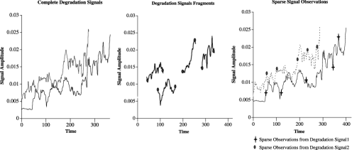
Recent developments in degradation modeling, such as Gebraeel et al. (2005), Liao, Zhao and Guo (2006), Zhou, Serban and Gebraeel (2011) and Zhou, Gebraeel and Serban (2012), have focused on utilizing degradation-based signals to predict lifetime or residual life distributions of engineering components. Almost all of the existing models rely on a historical database of degradation signals for estimating model parameters specifying the behavior of the degradation process. These signals can be acquired through a variety of methods. For instance, it may be possible to acquire frequent observations through extensive monitoring of a component over its life span, which results in a complete degradation signal. Another alternative is to follow an intermittent monitoring strategy, which leads to incomplete degradation signals. For instance, the degradation signals could be sparsely observed (i.e., sparse degradation signals) or densely observed over short time intervals (i.e., fragmented degradation signals). An example of complete, sparse and fragmented degradation signals is provided in Figure 1 available from Zhou, Serban and Gebraeel (2011).

More generally, components may be operated under different environmental conditions, for instance, different levels of humidity, speeds, loads and temperatures, among others. Environmental conditions can significantly accelerate or decelerate the degradation processes of functioning components. For example, in Gebraeel and Pan (2008), bearings are run at different rotating rates and, as a result, these bearings degrade at significantly different rates. However, most existing literature on degradation modeling assumes that components are from the same population and are operated under the same environmental conditions. An approach that does take the environmental conditions into account is commonly used for modeling accelerated degradation test (ADT) data. Whitmore and Schenkelberg (1997) propose a Wiener diffusion process with a time-scale transformation that depends upon the level of stress under which the ADT signals data are observed. Similar ideas can be found in Doksum and Hóyland (1992), Liao and Tseng (2006), Park and Padgett (2006) and Tseng, Balakrishnan and Tsai (2009). Other approaches that incorporate environmental data in degradation models include Kharoufeh (2003), Kharoufeh and Cox (2005), Li and Luo (2005) and Singpurwalla (1995). One common characteristic among these existing methods is that the dependence of the degradation processes on the environmental conditions is specified using a parametric functional form that describes how the degradation processes evolve over time; see Bae and Kvam (2004), Gebraeel (2006), Lawless and Crowder (2004), Meeker and Escobar (1998), Robinson and Crowder (2000), Wang and Xu (2010) and Whitmore, Crowder and Lawless (1998), among others.

In some applications, the underlying physics of degradation processes indeed may be known in advance. However, in many applications it may be difficult to identify a parametric model that can accurately capture the underlying trend of degradation processes. To overcome this challenge, recent research has considered nonparametric degradation models, in which the functional form is learned from the degradation data. Shiau and Lin (1999) applied nonparametric regression techniques to characterization of degradation signals of a light emitting diode product under different stress levels. Müller and Zhang (2005) proposed a time-varying regression approach for predicting the remaining lifetime of flies based on the observed reproductive activity. Both research works, however, assume that the degradation signals are completely observed. In Liao and Sun (2011), Zhou, Serban and Gebraeel (2011) and Zhou, Gebraeel and Serban (2012), the authors pointed out that the challenge is even more noteworthy when there are only incomplete degradation signals available. To overcome this challenge, they developed nonparametric degradation models based on functional data analysis and demonstrated that these models are generally more flexible and more robust to model misidentifications. These nonparametric models apply to signals observed at a small number of nonregularly sampled time points given that the number of degradation signals is sufficiently large.

In this paper, we develop a nonparametric model that does not require the functional form of mean degradation trend to be known in advance. This allows for more flexibility in modeling as compared to parametric approaches such as Lu and Meeker (1993) and other references mentioned above. More specifically, we build our modeling framework based upon functional data analysis (FDA) techniques. Functional data analysis is a collection of statistical techniques that focus on analyzing data in the form of curves, surfaces or functions. Examples of FDA methodologies include functional principal component analysis in Yao, Müller and Wang (2005), functional regression analysis in Ramsay and Dalzell (1991), functional time warping analysis in Telesca and Inoue (2008) etc. A comprehensive review and discussions of FDA methods and applications can be found in Ramsay and Silverman (2005). In this paper, we apply FDA techniques to different types of degradation signals, whether they are complete or incomplete, that specify the effects of varying environmental conditions on degradation processes within a flexible framework not requiring prior knowledge about the behavior of the degradation trend. Using a similar Bayesian framework as in Zhou, Serban and Gebraeel (2011), Zhou, Gebraeel and Serban (2012) but implemented within the model specifications in this paper, we predict and update in real time the residual life distributions (RLD) of components operated in the field, referred to as fielded components, by using their partially observed degradation signals. Unlike previous work by Zhou et al. (2014), the model presented in this paper allows for the degradation signals to be observed under varying environment conditions.

Specifically, we assume that the environmental conditions can be categorized into discrete types, and they are time invariant. Under this assumption, we consider two different scenarios. One scenario is supervised learning, in which the environmental types for all the training signals are available. In this case, only the new test (fielded) component’s environmental type is unknown and needs to be predicted. Another scenario is unsupervised learning, in which the environmental information is not available in advance. Under the second scenario, we also need to learn the clustering of the different environments along with the estimation of the degradation process corresponding to each group of environments. In both scenarios, the degradation model includes a random variable describing the cluster membership or the type of environmental conditions. In the second scenario, this variable is latent or missing.

Because we have two sources of missing data, one due to the fact the signals are thresholded and the second due to the missing cluster membership or unknown environment type, we propose using an Expectation–Maximization algorithm to estimate and update the distribution of the degradation process. The EM-type algorithm is a more flexible approach to model estimation when signals come from different environments.

The performance of the developed degradation framework is demonstrated by using both simulated degradation signals and a case study from a rotating machinery setup. We consider extensive types of scenarios, for instance, the components may be operated under known or unknown types of environmental conditions; the degradation signals may be complete or incomplete; the underlying degradation trend may or may not be expanded from the basis functions we specify. The results indicate that the proposed framework is quite flexible and can accurately predict the RLD of components operated in the field under all these scenarios.

The remaining paper is organized as follows. We first discuss the general model in Section 2. We present the details of the estimation approach in Section 3 followed by model prediction in Section 4. To assess the performance of our methodology, we continue with a simulation study and a case study in Sections 5 and 6, respectively. Conclusions and some discussions are given in Section 7. Technical details are provided in the supplemental material [Zhou, Serban and Gebraeel (2014)].

2 The model

2.1 Model decomposition

Denote the degradation level at time $t$ by $S(t)$, the failure threshold by $D$ and the environmental type by $Z$. According to the definition of failure, the lifetime of a component, denoted by $T$, is

$$T=\inf_{t}\bigl{\{}S(t)\geq D\bigr{\}}.$$ (1)

Here, $T$ is random and not observable due to the incompleteness and discreteness of the observed degradation signals.

In this paper, we consider a nonparametric decomposition of $S(\cdot)$, by assuming that it can be represented by a set of basis functions $B(\cdot)$, with a vector coefficient denoted by $\gamma$. We also assume that the environmental conditions are specified by the variable $Z$. Based on these assumptions, we consider estimating the degradation model using a likelihood based approach. The likelihood decomposition used in our model estimation is motivated by the fact that $T$ is unobservable. The decomposition is

$${L}(S,Z,\gamma)=f(Z)f(\gamma|Z)f(S|Z,\gamma),$$

where $Z$ and $\gamma$ are latent variables and, thus, we need to impose a parametric structure on both $Z$ and $\gamma|Z$. It is natural to assume that $Z$ follows a multinomial distribution, as the contribution of each environment type will be given by the probabilities of the multinomial distribution. This assumption in turn specifies that $S(\cdot)$ is a mixture process. Furthermore, the proportional parameters of the multinomial distribution can be estimated by the fraction of each cluster in the historical data set or determined by prior knowledge.

The distribution of $f(\gamma|Z)$ can be approximated by, for instance, a Gaussian distribution. This implies that, unconditionally, $\gamma$ follows a mixture of Gaussian distributions. The number of mixtures is equal to the number of different values $Z$ can take corresponding to the number of different environments. Other parametric assumptions can be considered at the price of a higher computation cost.

The second step is to specify $f(S|Z,\gamma)$. In our model specification in Section 2.2, the observed degradation signal is a sum of the underlying degradation process, which is completely determined by the basis coefficient $\gamma$ and a measurement error term. Therefore, $f(S|Z,\gamma)$ is fully determined by the distributional assumption about the measurement error. For ease of computational efficiency and for a close form expression of the RLD predictions, we assume the error term to follow a Gaussian distribution.

Given these specifications, we can predict the residual life of the component operated in the field in two steps. The first step is to predict $f(\gamma|S)$, the posterior distribution of $\gamma$ given the partial observations of the component still operated in the field. At the second step, the RLD of the operated component can then be predicted following the definition of the failure time in (1).

2.2 Modeling degradation signals

Denote the measurement (or inspection) time by $t_{lj}$, where $l=1,\ldots,L$ ($L$ is the number of signals or components) and $j=1,\ldots,n_{l}$ ($n_{l}$ is the number of observation time points for component $l$). We assume that the time points are prespecified within a bounded interval $[0,M]$, where $M$ refers to the maximum experimental time. The degradation amplitudes of the component $l$ are denoted by $S_{l}=(S_{l}(t_{lj}),\ldots,S_{l}(t_{ln_{l}}))$.

Note that $S_{l}(t_{lj})$ may not always be observable. For instance, a component may be shut down or replaced instantaneously after its degradation level reaches the failure threshold. In other words, no further observations can be acquired beyond the failure threshold. These types of signals are referred to as truncated degradation signals in Zhou, Serban and Gebraeel (2011). In these applications, $S_{l}(t_{lj})$ is observable only if the component $l$ has not failed by time $t_{lj}$.

We assume that the underlying degradation process, denoted by $X(\cdot)$, can be represented by a fixed number of basis functions. Based on this assumption, we consider the following degradation model specifying the conditional distribution $f(S|Z,\gamma)$:

$$S_{l}(t)=X_{l}(t)+\varepsilon_{l}(t)=B(t)\gamma_{l}+\varepsilon_{l}(t),$$ (2)

where:

• $X_{l}(\cdot)$ represents the underlying degradation process.

• $B(\cdot)$ represents the basis functions of dimension $q$, defined over the time interval $[0,M]$. For illustrative purposes, we use the cubic B-spline bases because of its flexibility. A B-spline function is a function that is connected by polynomial pieces with specified orders (“cubic” corresponds to the order 4). Cubic B-spline bases have been widely used in the literature for modeling smooth functions [Eilers and Marx (1996)].

• $\gamma_{l}$ represents the basis coefficient for the $l$th signal. It is a vector of dimension z$q$.

• $\varepsilon(\cdot)$ represents the error term. We assume that $\varepsilon(\cdot)$ is independent and identically distributed at different time points.

2.3 Modeling environmental clusters

In this paper we assume a component’s environmental type is time invariant, that is, it does not change over time. Let the environmental type for component $l$ be $Z_{l}\in\{1,2,\ldots,K\}$, where $K$ represents the number of environmental types or clusters (in the remaining paper, “environmental types” and “clusters” will be used interchangeably). We make the following distributional assumptions:

• $Z_{l}$ follows a multinomial distribution with parameters $\pi=(\pi_{1},\ldots,\pi_{K})$.

• Conditional on $Z_{l}$, the basis coefficient $\gamma$ follows a normal distribution. The distributional means and variances are different among environmental types. More specifically, $\gamma_{l,k}\equiv\gamma_{l}|Z_{l}=k\sim N(\mu_{k},\Lambda_{k})$, where ${\bolds\mu}_{k}=({\bolds\mu}_{k1},\ldots,{\bolds\mu}_{kq})^{T}$ and $\Lambda_{k}$ is a $q\times q$ matrix.

• Conditional on $Z_{l}$, the error terms are assumed to follow a normal distribution. The variances are different across clusters. In other words, $\varepsilon_{l}(t)|Z_{l}=k\sim N(0,\sigma_{k}^{2})$.

In summary, we have the following model:

$$\cases{\displaystyle Z_{l}\sim\operatorname{Multinomial}(\pi_{1},\ldots,\pi_{K}),\vspace*{3pt}\cr\displaystyle\gamma_{lk}\equiv\gamma_{l}|(Z_{l}=k)\sim N(\mu_{k},\Lambda_{k}),\vspace*{3pt}\cr\displaystyle S_{l}(t)=B(t)\gamma_{l}+\varepsilon_{l}(t),\vspace*{3pt}\cr\displaystyle\varepsilon_{l}(t)|(Z_{l}=k)\sim N\bigl{(}0,\sigma_{k}^{2}\bigr{)}.}$$ (3)

Based on the above formulation, we have $S_{l}(t)|Z_{l}=k\sim N(B(t)\mu_{k}$,$B(t)\Lambda_{k}B(t)^{T}+\sigma_{k}^{2}I)$.

3 Estimation

As mentioned earlier, we will consider two possible scenarios, that is, the cluster membership for the training components may or may not be known a priori. In the machine learning context, this corresponds to classification and clustering problems, respectively.

Let $\mu=(\mu_{1},\ldots,\mu_{K})$, $\Lambda=(\Lambda_{1},\ldots,\Lambda_{K})$, $\pi=(\pi_{1},\ldots,\pi_{K})$, $\sigma=(\sigma_{1},\ldots,\sigma_{K})$. The vector $\theta=(\mu,\Lambda,\pi,\sigma)$ includes all the parameters of the model in (3). Because of the presence of latent variables, it is intractable to maximize the complete data log-likelihood directly with respect to these parameters. To address this challenge, we apply an EM algorithm in order to obtain the maximum likelihood estimate of $\theta$. The estimation procedures are similar for the classification and clustering scenarios, except for an extra step in the clustering case, in which we classify all the training units. Details about the estimation algorithm are provided in the supplemental material [Zhou, Serban and Gebraeel (2014)]. In the following subsections, we highlight the challenge of estimating the covariance matrix $\Lambda$ and discuss how to determine the tuning parameters.

3.1 Estimating the covariance matrix

To allow for more flexibility, we assume that $\Lambda_{k}$ are different across clusters. This implies that we need to estimate $\frac{{Kq(q+1)}}{2}$ parameters for the covariance matrix. If we do not have a sufficiently large historical data set for training, then the covariance matrix estimate will be unstable and inaccurate. To overcome this challenge, we follow the idea of regularized discriminant analysis (RDA) proposed in Friedman (1989). More specifically, we regularize the raw covariance matrix estimates in two steps:

[Step 2.]

Shrink the individual sample covariance matrix estimate (${\hat{\Lambda}_{k}}$) toward the population sample covariance matrix estimate (${\hat{\Lambda}}$) with a parameter $0\leq\lambda\leq 1$:

$${{\hat{\Lambda}}_{k}}(\lambda)=(1-\lambda){{\hat{\Lambda}}_{k}}+\lambda\hat{\Lambda}.$$

Shrink ${\hat{\Lambda}_{k}}(\lambda)$ toward a multiple of the identity matrix with a parameter $0\leq\zeta\leq 1$:

$${{\hat{\Lambda}}_{k}}(\lambda,\zeta)=(1-\zeta){{\hat{\Lambda}}_{k}}(\lambda)+\zeta\frac{{\operatorname{tr}({{\hat{\Lambda}}_{k}}(\lambda))}}{p}I.$$

Friedman (1989) demonstrates through numerous case studies that ${{\hat{\Lambda}}_{k}}(\lambda,\zeta)$ is generally more stable and more accurate than the raw covariance matrix estimate ${\hat{\Lambda}_{k}}$, especially when the sample size of certain clusters is not large enough.

3.2 Choice of tuning parameters

The degradation model presentedabove depends on a series of tuning parameters: the basis dimension $q$, the shrinkage parameters $\lambda$ and $\zeta$, and possibly the number of clusters $K$ (for the clustering scenario). With larger values of $q$ and $K$, we have more parameters to estimate, resulting in smaller estimation bias but higher estimation variance. Thus, we need to select these parameters in order to optimize the bias-variance trade-off in the model.

To reduce the computational burden, we determine the turning parameters in two steps. We first select $q$ and possibly $K$ from a set of candidate values by following a cross-validation procedure. Cross-validation is a model validation technique for assessing how accurately a predictive model will perform in an independent data set. A detailed explanation of the cross-validation procedures can be found in Hastie, Tibshirani and Friedman (2009).

In our context, we compute the RLD prediction error for each combination of the candidate values in the cross-validation process. Based on the error results, we choose the combination of $q$ and $K$ that yields the smallest error. In the second step, we follow a similar cross-validation procedure to determine the optimal values of $\lambda$ and $\zeta$. The number of candidate values for these parameters determines the computation time for finding the optimal values. It is common to start with a rough set of candidate values that would provide an approximate range for the optimal values and then refine it with sample points within that range.

4 Prediction

Given the degradation signal $S^{*}$ of a new component operated in the file observed up to time $t^{*}$, our goal is to predict its residual life $\mbox{RL}^{*}$, that is, the time left for the signal to reach the failure threshold $D$. In other words, we need to derive the density function $f({\mbox{RL}^{*}}|{S^{*}})$. We approach this in two steps according to the following equation:

$$f\bigl{(}{\mbox{RL}^{*}}|{S^{*}}\bigr{)}=\int_{{\gamma}}{f\bigl{(}{\mbox{RL}^{*}}|{\gamma},{S^{*}}\bigr{)}f\bigl{(}{\gamma}|{S^{*}}\bigr{)}\,d{\gamma.}}$$

[Step 2.]

Compute ${f({\gamma}|{S^{*}}):}$

$$f\bigl{(}{\gamma}|{S^{*}}\bigr{)}=\sum_{k=1}^{K}{f\bigl{(}{\gamma}|{Z^{*}}=k,{S^{*}}\bigr{)}P\bigl{(}{Z^{*}}=k|{S^{*}}\bigr{)}.}$$

[(3)]

${{\gamma}|{Z^{*}}=k,{S^{*}}}$ follows a Gaussian distribution. Its mean vector and covariance matrix can be computed based on the general Bayesian linear theory. Details can be found in the supplemental material [Zhou, Serban and Gebraeel (2014)].

${Z^{*}}=k|{S^{*}}$ follows a multinomial distribution with its proportional parameters derived as follows. Since ${S^{*}}|{Z^{*}}=k\sim N(B{\mu_{k}},B{\Lambda_{k}}{B^{T}}+{\sigma_{k}^{2}}I)$, we have

$$P\bigl{(}{Z^{*}}=k|{S^{*}}\bigr{)}$$

$$\qquad=\frac{{f({S^{*}}|{Z^{*}}=k){\pi_{k}}}}{{\sum_{j=1}^{K}{f({S^{*}}|{Z^{*}}=j){\pi_{j}}}}}$$ (4)

$$\qquad=\biggl{(}\bigl{|}B{\Lambda_{k}}{B^{T}}+\sigma_{k}^{2}I\bigr{|}^{-1/2}$$

$$\hskip 38.0pt{}\times\exp\Biggl{(}-\frac{1}{2}\bigl{(}{S^{*}}-B{\mu_{k}}\bigr{)}^{T}\bigl{(}B{\Lambda_{k}}{B^{T}}+\sigma_{k}^{2}I\bigr{)}^{-1}\bigl{(}{S^{*}}-B{\mu_{k}}\bigr{)}\Biggr{)}{\pi_{k}}\biggr{)}$$

$$\quad\qquad{}\Big{/}\Biggl{(}\sum_{j=1}^{K}\bigl{|}{B{\Lambda_{j}}{B^{T}}+\sigma_{j}^{2}I}\bigr{|}^{-1/2}$$

$$\hskip 61.0pt{}\times\exp\biggl{(}-\frac{1}{2}{{\bigl{(}{S^{*}}-B{\mu_{j}}\bigr{)}}^{T}}{{\bigl{(}B{\Lambda_{j}}{B^{T}}+\sigma_{j}^{2}I\bigr{)}}^{-1}}\bigl{(}{S^{*}}-B{\mu_{j}}\bigr{)}\biggr{)}{\pi_{j}}\Biggr{)}.$$

Compute $f({\mbox{RL}^{*}}|{S^{*}})$: since $f({\mbox{RL}^{*}}|{S^{*}})$ does not have a closed-form expression, we suggest using a parametric bootstrap [Efron and Tibshirani (1993)] to generate samples from $f({\mbox{RL}^{*}}|{S^{*}})$ as follows:

[(5)]

Generate a random sample $\gamma$ from $f({\gamma}|{S^{*}})$ according to the density function given in step 1 (both ${\gamma}|{Z^{*}}=k,{S^{*}}$ and ${Z^{*}}=k|{S^{*}}$ follow a well-defined distribution that can be generated from existing statistical packages).

Generate the corresponding signal $S_{b}\dvtx S_{b}(t)=B(t)\gamma$.

Get the residual life ${\mbox{RL}_{b}}$ for the generated signal according to the failure time definition: ${\mbox{RL}_{b}}=\inf_{t}\{{S_{b}}(t)>D\}-t^{*}$.

If $\mbox{RL}_{b}>0$, then proceed to the next step; otherwise, repeat the above steps until $\mbox{RL}_{b}>0$.

Repeat the above steps for $N_{b}$ times and get $N_{b}$ values of $\mbox{RL}^{*}\dvtx\mathbf{RL}=(\mbox{RL}_{1},\mbox{RL}_{2},\ldots,\mbox{RL}_{N_{b}})$.

$\mathbf{RL}$ can then be used for the estimation of any statistics related to $\mbox{RL}^{*}$, such as quantiles and prediction intervals.

5 Simulation study

5.1 Simulation setting

In this study, we assume that components are from two different clusters, that is, they are operated under two different environmental types. We first simulate the cluster membership $Z_{l}$ from a Binomial distribution with equal parameters, that is, $Z_{l}\sim\operatorname{Binomial}(\pi_{1}=0.5,\pi_{2}=0.5)$. Next, we generate signals from each cluster based on the following model settings:

• In cluster $1$, $S_{l}(t)=\mu(t)+X_{l}(t)+\varepsilon_{l}(t)$, where:

  • $\mu(t)=4t^{2}e^{t/25}$, which represents the overall mean degradation trend for components within this cluster.

  • $X_{l}(t)=\beta_{l}t^{2}$, which is introduced to account for the unit to unit heterogeneity in degradation. Here, $\beta_{l}\sim N(0,1.5^{2})$.

  • $\varepsilon(t)|(Z_{l}=2)\sim N(0,60^{2})$.

• In cluster $2$, $S_{l}(t)=B(t)\gamma_{l}+\varepsilon(t)$, where:

  • $B(\cdot)$ represents the cubic B-spline basis with its dimension $q=5$.

  • $\gamma_{l}\sim N(\mu_{1},\Sigma_{1})$, where $\mu_{1}=(0,500,1500,2500,3000)$ and

    $$\Sigma_{1}^{-1}={\Omega_{1}}/{5600};\qquad{{\Omega_{1}}}=\pmatrix{2&{-1}&0&0&0\cr{-1}&2&{-1}&0&0\cr 0&{-1}&2&{-1}&0\cr 0&0&{-1}&2&{-1}\cr 0&0&0&{-1}&1}_{5\times 5}.$$

    The value of $\mu_{1}$ ensures that the overall mean degradation trend of this cluster is linear. The underlying degradation process of each component can still be nonlinear. A covariance matrix of similar structure to $\Sigma_{1}$ is frequently used as a prior for the basis coefficients under the Bayesian framework [Lang and Brezger (2004)]. Under the frequentist framework, this corresponds to penalized regression splines [Eilers and Marx (1996)].

  • $\varepsilon(t)|(Z_{l}=1)\sim N(0,80^{2})$.

We note that the signals in cluster $2$ are generated under the general framework proposed in equations (3), while the signals within cluster $1$ are not.

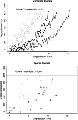
Based on the above model settings, we generate $100$ signals for training the degradation model and another $100$ signals for evaluating the RLD prediction performance of our model. All the signals are truncated at the failure threshold, which is $D=1000$ for both clusters. We evaluate the performance of our methodology under complete as well as sparse scenarios. For a complete signal, the measurement time points are preset at an equally spaced grid ${c_{0},\ldots,c_{80}}$ on $[0,20]$ with $c_{0}=0,c_{80}=20$. For a sparse signal, we uniformly sample $12$ time points from ${c_{0},\ldots,c_{80}}$. Note that these time points are prespecified; due to truncation, degradation signals at these time points are not always observable. In this simulation, we have around $40$ observations per complete signal and only around $6$ observations per sparse signal. Examples of the generated complete and sparse degradation signals can be found in Figure 2. In both plots, the black lines/dots represent the signals from cluster $1$ and the grey lines/dots represent the signals from cluster $2$.

5.2 Estimation

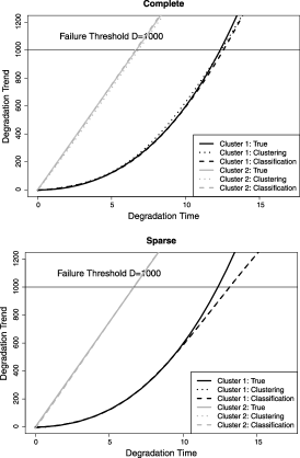
Based on the generated complete or sparse signals, we can estimate the mean degradation trend for each cluster. The results are shown in the top and bottom plots of Figure 3. In both plots, the solid, dotted and dashed lines represent the true mean trend, the estimated trend in the clustering scenario and the estimated trend in the classification scenario, respectively. From Figure 3, we observe that the estimated mean degradation trend for both classification and clustering scenarios are very close to the true trend (except for a small departure in the first cluster under the sparse case, which is mainly due to the limited data available in that region). This indicates that the mean functions are estimated accurately for both classification and clustering scenarios and under both complete and sparse cases.

Figure 2: Examples of complete (top plot) and sparse (bottom plot) degradation signals.

Figure 3: Estimated (true, classification, clustering) mean function for the complete and sparse scenarios, respectively.

In the clustering scenario, we are also interested in whether the training signals are clustered accurately. To this purpose, we compute the Rand index measuring the percentage of pairs of components on which two clusterings, denoted by $X_{1}$ and $X_{2}$, agree or disagree [Rand (1971)]. Generally, $\operatorname{Rand}({X_{1}},{X_{2}})$ ranges from $0$ when there are no pairs classified in the same class under $X_{1}$ and $X_{2}$, to $1$ when $X_{1}$ and $X_{2}$ give identical clustering. Here we use $X_{1}$ to denote the true cluster membership of the 100 training signals generated in one run of simulation and $X_{2}$ to denote the grouping estimated using our proposed clustering method. Under both complete and sparse scenarios, $\operatorname{Rand}({X_{1}},{X_{2}})=1$, which indicates that our clustering method performs well under both scenarios for the generated 100 training signals. Accurate grouping of signals results in a better prediction of RLD for fielded components.

The clustering performance is dependent upon many factors, for instance, the mixing level of signals from different clusters. For illustrative purposes, we perform a sensitivity analysis provided in the supplemental material [Zhou, Serban and Gebraeel (2014)].

5.3 Prediction

Our next step is to evaluate the performance of our model in terms of residual life prediction. To assess the prediction accuracy, we use the mean squared prediction error criteria because the posterior mean (i.e., the expectation of the posterior predictive distribution) is used as the point prediction. For each testing component, we compute the prediction errors at the following percentiles of its entire life: 10%, 30%$,\ldots,90$% (90% implies that 90% of the component’s life has passed). The results based on complete and sparse signals are illustrated in Figures 4 and 5, respectively. In both figures, the top left and top right plots are for the classification and clustering cases. For comparative purposes, we also use a benchmark method, which is based on our proposed framework (including the estimation and prediction approaches). In the benchmark method all the components are assumed to come from the same population and, therefore, it does not account for the two different environmental types. We refer to this benchmark method as “no clustering.” The results of “no clustering” are reported in the bottom plots of Figures 4 and 5. For ease of comparison, we also summarize the results in Table 1, which gives the mean and the variance of prediction errors for different methods based on complete and sparse degradation signals.

Figure 4: Mean squared prediction errors for “classification,” “clustering” and “no clustering” based on complete degradation signals.

Figure 5: Mean squared prediction errors for “classification,” “clustering” and “no clustering” based on sparse degradation signals.

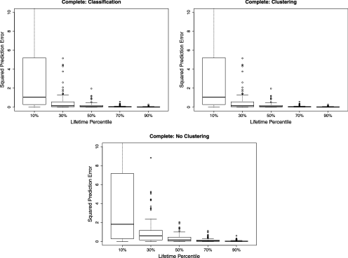
One consistent observation from the figures and tables is that the prediction results are very similar for the classification and clustering scenarios. This again demonstrates that, at least in this simulation, our proposed clustering algorithm can accurately classify signals of similar patterns into the same group and separate signals of distinct patterns into different groups. Furthermore, the benchmark method provides less accurate predictions of the residual life of components operated in the field. This is because the assumption that all components are from the same population does not hold in this simulation. The difference in performance between our methods and the benchmark method “no clustering” is more significant at smaller life percentiles, when the prior distribution plays a relatively more important role in the RLD predictions.

Table 1: Lifetime prediction results of “classification,” “clustering” and “no clustering” under complete and sparse scenarios

Lifetime percentiles	10%	30%	50%	70%	90%
Complete: classification	3.24	0.58	0.21	0.10	0.06
Complete: clustering	3.24	0.58	0.21	0.10	0.06
Complete: no clustering	4.58	1.08	0.45	0.18	0.08
Sparse: classification	6.18	1.09	0.62	0.53	0.34
Sparse: clustering	6.41	1.11	0.64	0.54	0.34
Sparse: no clustering	7.52	1.67	1.33	0.65	0.33

6 Bearing case study

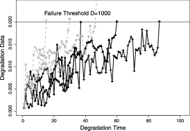
Bearings play an important role in a wide range of engineering applications, particularly in rotating machinery. Failures of bearings can lead to unexpected shutdown or failure of the entire engineering system. In this study, we conduct an experiment to monitor the degradation processes of rolling bearings. Each bearing is operated under one of the following two rotational levels: $2200$ r.p.m. and $2600$ r.p.m. (r.p.m. is shorted for “revolutions per minute”). The sample size of each cluster is $16$ and $18$, respectively. For all bearings, we collect vibration-based degradation signals up to their failures. The failure threshold is prespecified as $D=0.02$ v.r.m.s. (v.r.m.s. is shorted for “vibrational root mean square”). Examples of the resulting degradation signals are in Figure 6. In this figure, the solid lines represent the degradation signals from cluster 1 ($2200$ r.p.m.) and the dashed lines represent those from cluster 2 ($2600$ r.p.m.).

Figure 6: Examples of bearing degradation signals.

Figure 7: Estimated mean degradation trend under the classification and clustering scenarios.

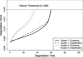
To evaluate the performance of our proposed degradation model, we repeat the following study for $50$ times. Each time we randomly select $5$ signals from each cluster as the testing signals. For these testing signals, we assume that their cluster membership, or rotational speed, is unknown and needs to be predicted. They are used to assess the prediction performance. The rest of the $24$ degradation signals ($11$ of them are from cluster 1 and the rest of the $13$ signals are from cluster 2) form a historical data set and they are used to train the proposed degradation model and estimate the parameters. Depending on the scenario we are interested in, whether it is “classification” or “clustering,” the cluster membership of the training components may or may not be known. In Figure 7, we show the estimated mean degradation trend (up to the failure threshold) for both clusters. Apparently, the degradation processes in cluster 2 with a rotational speed of $2600$ r.p.m. are relatively faster than those from cluster 1 with a rotational speed of $2200$ r.p.m. Another observation is that the estimated mean degradation trend under the classification and clustering scenarios is similar.

Figure 8: Prediction errors under the classification and clustering scenarios.

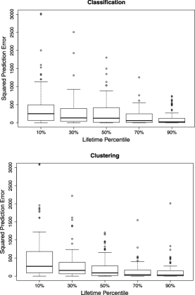
To mimic and illustrate the real-time updating process, we also assess the prediction performance progressively. More specifically, for each test bearing, we predict its residual life by using the partially observed signal at the following percentiles of its lifetime: $10\%$, $30\%,\ldots,90\%$. As the percentile gets larger, we have more degradation observations available and, therefore, we expect to see more accurate and more precise predictions of the RLD. This is demonstrated in the boxplots of Figure 8, in which we consider both the classification and clustering scenarios. In these boxplots, the $x$-axis represents the lifetime percentiles and the $y$-axis records the mean squared prediction errors. We observe that both the median and variance of the prediction errors decrease as the lifetime percentile increases, and this is consistent with our observations from the simulation study. Another observation from Figure 8 is that the prediction performance for the classification and clustering scenarios is very similar. This, once again, demonstrates that our proposed clustering algorithm can classify degradation signals quite accurately.

7 Summary

In this paper we propose a nonparametric model for characterizing the evolution of degradation signals under varying experimental or environmental conditions. This model can be used for predicting the lifetime or residual life distributions of engineering components that are still operated in the field. Our proposed framework relies on a series of assumptions as follows:

[(3)]

The underlying degradation process is smooth.

The degradation signals follow a Gaussian process with nonparametric mean and covariance.

The environmental conditions can be categorized into a discrete number of groups.

The environmental conditions are constant over time.

In this paper we use the cubic B-spline basis due to its flexibility. Other choices of basis functions can also be used depending on specific assumptions on the smoothness of the degradation process. In our simulation study, we observe that the estimation and prediction performance of our model is robust to the departures from this assumption (degradation signals from the first cluster cannot be linearly expanded by the cubic B-spline basis functions). Nonetheless, the use of cubic B-splines implies that the degradation is smooth over time, which may not hold in all applications.

Our proposed model is nonparametric in the sense that the mean and covariance of the Gaussian process specifying the conditional distribution $S(\cdot)|Z$ are assumed not to have a predefined parametric structure. This is a common approach in functional data analysis. We have investigated the impact of departures from the Gaussian assumption in a sensitivity study (not reported in the paper but available from the authors). According to our sensitivity analysis, the RLD prediction errors are more sensitive to the accuracy of the estimated degradation trend functions compared to these distributional assumptions.

The third assumption mentioned above may not always hold in real world applications. In such cases, it may be more appropriate to consider the environmental condition as a continuous covariate rather than discrete clusters. We may still follow the general decomposition of the degradation process in equation (2), but the classification or clustering framework in equation (3) will not be applicable. One possible approach is to follow similar ideas used in modeling the ADT data, that is, by assuming certain functional, either linear or nonlinear, relationships between the basis coefficient $\gamma_{l}$ and the environmental variable $Z_{l}$.

In certain applications, the environmental conditions could be time varying [Bian and Gebraeel (2013); Gebraeel and Pan (2008)]. For instance, the cluster membership $Z_{l}$ may change at certain deterministic or random time epochs. At these transitional epochs, the observed degradation signals may be subject to sudden shocks, and the rate at which the degradation progresses may also change. A further extension of the present framework to incorporate such time-varying environmental conditions will be of interest in our future research.

References

- Bae and Kvam (2004) {barticle}[mr] \bauthor\bsnmBae, \bfnmSuk Joo\binitsS. J. and \bauthor\bsnmKvam, \bfnmPaul H.\binitsP. H. (\byear2004). \btitleA nonlinear random-coefficients model for degradation testing. \bjournalTechnometrics \bvolume46 \bpages460–469. \biddoi=10.1198/004017004000000464, issn=0040-1706, mr=2101514 \bptokimsref\endbibitem
- Bian and Gebraeel (2013) {barticle}[mr] \bauthor\bsnmBian, \bfnmLinkan\binitsL. and \bauthor\bsnmGebraeel, \bfnmNagi\binitsN. (\byear2013). \btitleStochastic methodology for prognostics under continuously varying environmental profiles. \bjournalStat. Anal. Data Min. \bvolume6 \bpages260–270. \biddoi=10.1002/sam.11154, issn=1932-1864, mr=3062269 \bptokimsref\endbibitem
- Doksum and Hóyland (1992) {barticle}[auto:STB—2014/06/18—12:29:53] \bauthor\bsnmDoksum, \bfnmK. A.\binitsK. A. and \bauthor\bsnmHóyland, \bfnmA.\binitsA. (\byear1992). \btitleModels for variable-stress accelerated life testing experiments based on Wiener processes and the inverse Gaussian distribution. \bjournalTechnometrics \bvolume34 \bpages74–82. \bptokimsref\endbibitem
- Efron and Tibshirani (1993) {bbook}[mr] \bauthor\bsnmEfron, \bfnmBradley\binitsB. and \bauthor\bsnmTibshirani, \bfnmRobert J.\binitsR. J. (\byear1993). \btitleAn Introduction to the Bootstrap. \bpublisherChapman & Hall, \blocationNew York. \biddoi=10.1007/978-1-4899-4541-9, mr=1270903 \bptokimsref\endbibitem
- Eilers and Marx (1996) {barticle}[mr] \bauthor\bsnmEilers, \bfnmPaul H. C.\binitsP. H. C. and \bauthor\bsnmMarx, \bfnmBrian D.\binitsB. D. (\byear1996). \btitleFlexible smoothing with B-splines and penalties. \bjournalStatist. Sci. \bvolume11 \bpages89–121. \biddoi=10.1214/ss/1038425655, issn=0883-4237, mr=1435485 \bptnotecheck related \bptokimsref\endbibitem
- Friedman (1989) {barticle}[mr] \bauthor\bsnmFriedman, \bfnmJerome H.\binitsJ. H. (\byear1989). \btitleRegularized discriminant analysis. \bjournalJ. Amer. Statist. Assoc. \bvolume84 \bpages165–175. \bidissn=0162-1459, mr=0999675 \bptokimsref\endbibitem
- Gebraeel (2006) {barticle}[auto:STB—2014/06/18—12:29:53] \bauthor\bsnmGebraeel, \bfnmN.\binitsN. (\byear2006). \btitleSensory updated residual life distribution for components with exponential degradation patterns. \bjournalIEEE Trans. Autom. Sci. Eng. \bvolume3 \bpages382–393. \bptokimsref\endbibitem
- Gebraeel and Pan (2008) {barticle}[auto:STB—2014/06/18—12:29:53] \bauthor\bsnmGebraeel, \bfnmN.\binitsN. and \bauthor\bsnmPan, \bfnmJ.\binitsJ. (\byear2008). \btitlePrognostic degradation models for computing and updating residual life distributions in a time-varying environment. \bjournalIEEE Trans. Reliab. \bvolume57 \bpages539–550. \bptokimsref\endbibitem
- Gebraeel et al. (2005) {barticle}[auto:STB—2014/06/18—12:29:53] \bauthor\bsnmGebraeel, \bfnmN.\binitsN., \bauthor\bsnmLawley, \bfnmM.\binitsM., \bauthor\bsnmLi, \bfnmR.\binitsR. and \bauthor\bsnmRyan, \bfnmJ.\binitsJ. (\byear2005). \btitleResidual-life distributions from component degradation signals: A Bayesian approach. \bjournalIIE Trans. \bvolume37 \bpages543–557. \bptokimsref\endbibitem
- Hastie, Tibshirani and Friedman (2009) {bbook}[mr] \bauthor\bsnmHastie, \bfnmTrevor\binitsT., \bauthor\bsnmTibshirani, \bfnmRobert\binitsR. and \bauthor\bsnmFriedman, \bfnmJerome\binitsJ. (\byear2009). \btitleThe Elements of Statistical Learning: Data Mining, Inference, and Prediction, \bedition2nd ed. \bpublisherSpringer, \blocationNew York. \biddoi=10.1007/978-0-387-84858-7, mr=2722294 \bptnotecheck year \bptokimsref\endbibitem
- Kharoufeh (2003) {barticle}[mr] \bauthor\bsnmKharoufeh, \bfnmJeffrey P.\binitsJ. P. (\byear2003). \btitleExplicit results for wear processes in a Markovian environment. \bjournalOper. Res. Lett. \bvolume31 \bpages237–244. \biddoi=10.1016/S0167-6377(02)00229-8, issn=0167-6377, mr=1967296 \bptokimsref\endbibitem
- Kharoufeh and Cox (2005) {barticle}[auto:STB—2014/06/18—12:29:53] \bauthor\bsnmKharoufeh, \bfnmJ. P.\binitsJ. P. and \bauthor\bsnmCox, \bfnmS. M.\binitsS. M. (\byear2005). \btitleStochastic models for degradation based reliability. \bjournalIIE Trans. \bvolume37 \bpages533–542. \bptokimsref\endbibitem
- Lang and Brezger (2004) {barticle}[mr] \bauthor\bsnmLang, \bfnmStefan\binitsS. and \bauthor\bsnmBrezger, \bfnmAndreas\binitsA. (\byear2004). \btitleBayesian P-splines. \bjournalJ. Comput. Graph. Statist. \bvolume13 \bpages183–212. \biddoi=10.1198/1061860043010, issn=1061-8600, mr=2044877 \bptokimsref\endbibitem
- Lawless and Crowder (2004) {barticle}[mr] \bauthor\bsnmLawless, \bfnmJerry\binitsJ. and \bauthor\bsnmCrowder, \bfnmMartin\binitsM. (\byear2004). \btitleCovariates and random effects in a gamma process model with application to degradation and failure. \bjournalLifetime Data Anal. \bvolume10 \bpages213–227. \biddoi=10.1023/B:LIDA.0000036389.14073.dd, issn=1380-7870, mr=2086957 \bptokimsref\endbibitem
- Li and Luo (2005) {barticle}[mr] \bauthor\bsnmLi, \bfnmGang\binitsG. and \bauthor\bsnmLuo, \bfnmJiaowan\binitsJ. (\byear2005). \btitleShock model in Markovian environment. \bjournalNaval Res. Logist. \bvolume52 \bpages253–260. \biddoi=10.1002/nav.20068, issn=0894-069X, mr=2124478 \bptokimsref\endbibitem
- Liao and Sun (2011) {barticle}[auto:STB—2014/06/18—12:29:53] \bauthor\bsnmLiao, \bfnmH.\binitsH. and \bauthor\bsnmSun, \bfnmJ.\binitsJ. (\byear2011). \btitleNonparametric and semi-parametric sensor recovery in multichannel condition monitoring systems. \bjournalIEEE Trans. Autom. Sci. Eng. \bvolume8 \bpages744–753. \bptokimsref\endbibitem
- Liao and Tseng (2006) {barticle}[auto:STB—2014/06/18—12:29:53] \bauthor\bsnmLiao, \bfnmC. M.\binitsC. M. and \bauthor\bsnmTseng, \bfnmS. T.\binitsS. T. (\byear2006). \btitleOptimal design for step-stress accelerated degradation tests. \bjournalIEEE Trans. Reliab. \bvolume55 \bpages59–66. \bptokimsref\endbibitem
- Liao, Zhao and Guo (2006) {bincollection}[auto:STB—2014/06/18—12:29:53] \bauthor\bsnmLiao, \bfnmH.\binitsH., \bauthor\bsnmZhao, \bfnmW.\binitsW. and \bauthor\bsnmGuo, \bfnmH.\binitsH. (\byear2006). \btitlePredicting remaining useful life of an individual unit using proportional hazards model and logistic regression model. In \bbooktitleReliability and Maintainability Symposium, 2006. RAMS’06. Annual. \bpages127–132. \bpublisherIEEE, \blocationNew York. \bptokimsref\endbibitem
- Lu and Meeker (1993) {barticle}[mr] \bauthor\bsnmLu, \bfnmC. Joseph\binitsC. J. and \bauthor\bsnmMeeker, \bfnmWilliam Q.\binitsW. Q. (\byear1993). \btitleUsing degradation measures to estimate a time-to-failure distribution. \bjournalTechnometrics \bvolume35 \bpages161–174. \biddoi=10.2307/1269661, issn=0040-1706, mr=1225093 \bptokimsref\endbibitem
- Meeker and Escobar (1998) {bbook}[auto:STB—2014/06/18—12:29:53] \bauthor\bsnmMeeker, \bfnmW. Q.\binitsW. Q. and \bauthor\bsnmEscobar, \bfnmL. A.\binitsL. A. (\byear1998). \btitleStatistical Methods for Reliability Data. \bpublisherWiley, \blocationNew York. \bptokimsref\endbibitem
- Müller and Zhang (2005) {barticle}[mr] \bauthor\bsnmMüller, \bfnmHans-Georg\binitsH.-G. and \bauthor\bsnmZhang, \bfnmYing\binitsY. (\byear2005). \btitleTime-varying functional regression for predicting remaining lifetime distributions from longitudinal trajectories. \bjournalBiometrics \bvolume61 \bpages1064–1075. \biddoi=10.1111/j.1541-0420.2005.00378.x, issn=0006-341X, mr=2216200 \bptokimsref\endbibitem
- Park and Padgett (2006) {barticle}[auto:STB—2014/06/18—12:29:53] \bauthor\bsnmPark, \bfnmC.\binitsC. and \bauthor\bsnmPadgett, \bfnmW. J.\binitsW. J. (\byear2006). \btitleStochastic degradation models with several accelerating variables. \bjournalIEEE Trans. Reliab. \bvolume55 \bpages379–390. \bptokimsref\endbibitem
- Ramsay and Dalzell (1991) {barticle}[mr] \bauthor\bsnmRamsay, \bfnmJ. O.\binitsJ. O. and \bauthor\bsnmDalzell, \bfnmC. J.\binitsC. J. (\byear1991). \btitleSome tools for functional data analysis. \bjournalJ. Roy. Statist. Soc. Ser. B \bvolume53 \bpages539–572. \bidissn=0035-9246, mr=1125714 \bptnotecheck related \bptokimsref\endbibitem
- Ramsay and Silverman (2005) {bbook}[mr] \bauthor\bsnmRamsay, \bfnmJ. O.\binitsJ. O. and \bauthor\bsnmSilverman, \bfnmB. W.\binitsB. W. (\byear2005). \btitleFunctional Data Analysis, \bedition2nd ed. \bpublisherSpringer, \blocationNew York. \bidmr=2168993 \bptokimsref\endbibitem
- Rand (1971) {barticle}[auto:STB—2014/06/18—12:29:53] \bauthor\bsnmRand, \bfnmW. M.\binitsW. M. (\byear1971). \btitleObjective criteria for the evaluation of clusterings methods. \bjournalJ. Amer. Statist. Assoc. \bvolume66 \bpages846–850. \bptokimsref\endbibitem
- Robinson and Crowder (2000) {barticle}[mr] \bauthor\bsnmRobinson, \bfnmMichael E.\binitsM. E. and \bauthor\bsnmCrowder, \bfnmMartin J.\binitsM. J. (\byear2000). \btitleBayesian methods for a growth-curve degradation model with repeated measures. \bjournalLifetime Data Anal. \bvolume6 \bpages357–374. \biddoi=10.1023/A:1026509432144, issn=1380-7870, mr=1823809 \bptokimsref\endbibitem
- Shiau and Lin (1999) {barticle}[auto:STB—2014/06/18—12:29:53] \bauthor\bsnmShiau, \bfnmJ. H.\binitsJ. H. and \bauthor\bsnmLin, \bfnmH.\binitsH. (\byear1999). \btitleAnalyzing accelerated degradation data by nonparametric regression. \bjournalIEEE Trans. Reliab. \bvolume48 \bpages149–158. \bptokimsref\endbibitem
- Singpurwalla (1995) {barticle}[auto:STB—2014/06/18—12:29:53] \bauthor\bsnmSingpurwalla, \bfnmN. D.\binitsN. D. (\byear1995). \btitleSurvival in dynamic environments. \bjournalStatist. Sci. \bvolume10 \bpages86–103. \bptokimsref\endbibitem
- Telesca and Inoue (2008) {barticle}[mr] \bauthor\bsnmTelesca, \bfnmDonatello\binitsD. and \bauthor\bsnmInoue, \bfnmLurdes Y. T.\binitsL. Y. T. (\byear2008). \btitleBayesian hierarchical curve registration. \bjournalJ. Amer. Statist. Assoc. \bvolume103 \bpages328–339. \biddoi=10.1198/016214507000001139, issn=0162-1459, mr=2420237 \bptokimsref\endbibitem
- Tseng, Balakrishnan and Tsai (2009) {barticle}[auto:STB—2014/06/18—12:29:53] \bauthor\bsnmTseng, \bfnmS. T.\binitsS. T., \bauthor\bsnmBalakrishnan, \bfnmN.\binitsN. and \bauthor\bsnmTsai, \bfnmC. C.\binitsC. C. (\byear2009). \btitleOptimal step-stress accelerated degradation test plan for gamma degradation processes. \bjournalIEEE Trans. Reliab. \bvolume58 \bpages611–618. \bptokimsref\endbibitem
- Wang and Xu (2010) {barticle}[mr] \bauthor\bsnmWang, \bfnmXiao\binitsX. and \bauthor\bsnmXu, \bfnmDihua\binitsD. (\byear2010). \btitleAn inverse Gaussian process model for degradation data. \bjournalTechnometrics \bvolume52 \bpages188–197. \biddoi=10.1198/TECH.2009.08197, issn=0040-1706, mr=2676425 \bptokimsref\endbibitem
- Whitmore, Crowder and Lawless (1998) {barticle}[auto:STB—2014/06/18—12:29:53] \bauthor\bsnmWhitmore, \bfnmG. A.\binitsG. A., \bauthor\bsnmCrowder, \bfnmM. I.\binitsM. I. and \bauthor\bsnmLawless, \bfnmJ. F.\binitsJ. F. (\byear1998). \btitleFailure inference from a marker process based on bivariate model. \bjournalLifetime Data Anal. \bvolume4 \bpages229–251. \bptokimsref\endbibitem
- Whitmore and Schenkelberg (1997) {barticle}[auto:STB—2014/06/18—12:29:53] \bauthor\bsnmWhitmore, \bfnmG. A.\binitsG. A. and \bauthor\bsnmSchenkelberg, \bfnmF.\binitsF. (\byear1997). \btitleModelling accelerated degradation data using Wiener diffusion with a time scale transformation. \bjournalLifetime Data Anal. \bvolume3 \bpages27–45. \bptokimsref\endbibitem
- Yao, Müller and Wang (2005) {barticle}[mr] \bauthor\bsnmYao, \bfnmFang\binitsF., \bauthor\bsnmMüller, \bfnmHans-Georg\binitsH.-G. and \bauthor\bsnmWang, \bfnmJane-Ling\binitsJ.-L. (\byear2005). \btitleFunctional data analysis for sparse longitudinal data. \bjournalJ. Amer. Statist. Assoc. \bvolume100 \bpages577–590. \biddoi=10.1198/016214504000001745, issn=0162-1459, mr=2160561 \bptokimsref\endbibitem
- Zhou, Gebraeel and Serban (2012) {barticle}[auto:STB—2014/06/18—12:29:53] \bauthor\bsnmZhou, \bfnmR.\binitsR., \bauthor\bsnmGebraeel, \bfnmN.\binitsN. and \bauthor\bsnmSerban, \bfnmN.\binitsN. (\byear2012). \btitleDegradation modeling and monitoring of truncated degradation signals. \bjournalIIE Trans. \bvolume44 \bpages793–803. \bptokimsref\endbibitem
- Zhou, Serban and Gebraeel (2011) {barticle}[mr] \bauthor\bsnmZhou, \bfnmRensheng R.\binitsR. R., \bauthor\bsnmSerban, \bfnmNicoleta\binitsN. and \bauthor\bsnmGebraeel, \bfnmNagi\binitsN. (\byear2011). \btitleDegradation modeling applied to residual lifetime prediction using functional data analysis. \bjournalAnn. Appl. Stat. \bvolume5 \bpages1586–1610. \biddoi=10.1214/10-AOAS448, issn=1932-6157, mr=2849787 \bptokimsref\endbibitem
- Zhou, Serban and Gebraeel (2014) {bmisc}[auto] \bauthor\bsnmZhou, \bfnmRensheng\binitsR., \bauthor\bsnmSerban, \bfnmNicoleta\binitsN. and \bauthor\bsnmGebraeel, \bfnmNagi\binitsN. (\byear2014). \bhowpublishedSupplement to “Degradation-based residual life prediction under different environments.” DOI:\doiurl10.1214/14-AOAS749SUPP. \bptokimsref\endbibitem
- Zhou et al. (2014) {barticle}[mr] \bauthor\bsnmZhou, \bfnmRensheng R.\binitsR. R., \bauthor\bsnmSerban, \bfnmNicoleta\binitsN., \bauthor\bsnmGebraeel, \bfnmNagi\binitsN. and \bauthor\bsnmMüller, \bfnmHans-Georg\binitsH.-G. (\byear2014). \btitleA functional time warping approach to modeling and monitoring truncated degradation signals. \bjournalTechnometrics \bvolume56 \bpages67–77. \biddoi=10.1080/00401706.2013.805661, issn=0040-1706, mr=3176573 \bptokimsref\endbibitem