Phase diagram of fluid phases in ${{}^{3}\text{He}}$ -${{}^{4}\text{He}}$ mixtures

Abstract

Fluid parts of the phase diagram of ${{}^{3}\text{He}}$ -${{}^{4}\text{He}}$ mixtures are obtained from a mean-field analysis of a suitable lattice gas model for binary liquid mixtures. The proposed model takes into account the continuous rotational symmetry O(2) of the superfluid degrees of freedom associated with ${{}^{4}\text{He}}$ and includes the occurrence of vacancies. This latter degree of freedom allows the model to exhibit a vapor phase and hence can provide the theoretical framework to describe the experimental conditions for measurements of tricritical Casimir forces in ${{}^{3}\text{He}}$ -${{}^{4}\text{He}}$ wetting films.

I INTRODUCTION

Binary mixtures of the helium isotopes ${{}^{3}\text{He}}$ and ${{}^{4}\text{He}}$ exhibit a very rich phase behavior due to the presence of pronounced quantum effects. For example, below a certain threshold value of the pressure the zero-point fluctuations of the helium atoms demolish the solid phase. Accordingly, the liquid phase persists down to temperature $T=0$. The solid phase forms only at high pressures, whereas for sufficiently low pressures and $T>0$ helium forms the vapor phase. The bulk phase diagram of ${{}^{4}\text{He}}$ is shown schematically in Fig. 1. The liquid phase can be either a normal fluid or superfluid. These two fluid phases are separated by a line of second-order phase transitions, which is called $\lambda$-line. This line terminates at the critical end points ce⁺ and ce at the liquid-solid and liquid-vapor coexistence lines, respectively. The liquid-vapor coexistence line terminates at the critical point c.
Adding ${{}^{3}\text{He}}$ atoms to the pure ${{}^{4}\text{He}}$ liquid, dilutes the ${{}^{4}\text{He}}$ carriers of superfluidity and thus lowers the critical temperature of the superfluid transition. (Superfluid transitions of ${{}^{3}\text{He}}$ atoms occur at very low temperatures, which are not considered here.) Beyond a certain dilution due to ${{}^{3}\text{He}}$ atoms the superfluid transition turns into a first-order phase transition; this occurs at a tricritical point tc. The schematic phase diagram of ${{}^{3}\text{He}}$ -${{}^{4}\text{He}}$ mixtures at fixed pressure is shown in Fig. 2. The transition temperature $T_{\lambda}$ of the second-order phase transition to the superfluid phase depends on the concentration $X_{3}$ of ${{}^{3}\text{He}}$ atoms. For temperatures below the tricritical point tc, the mixture undergoes a first-order superfluid-normal phase transition which is accompanied by a two-phase region.
The schematic phase diagram of ${{}^{3}\text{He}}$ -${{}^{4}\text{He}}$ mixtures in the $(T,Z,P)$ space, where $Z$ is the fugacity of ${{}^{3}\text{He}}$, is shown in Fig. 3 Krech and Dietrich (1992a). In the plane $Z=0$, i.e., in the case of pure ${{}^{4}\text{He}}$, the phase diagram is the same as the one in Fig. 1. $A_{1}$ and $A_{2}$ are the surfaces of first-order solid-liquid and vapor-liquid transitions, respectively, whereas $A_{3}$ and $A_{4}$ are the surfaces of second- and first-order phase transitions, respectively, between the superfluid and the normal fluid. Accordingly, $A_{3}$ and $A_{4}$ are separated by a line TC of tricritical points, which terminates at the tricritical end points tce⁺ and tce. The points tce⁺ and ce⁺ as well as tce and ce are connected by lines of critical end points on $A_{1}$ and $A_{2}$, respectively. The surface $A_{4}$ intersects the surfaces $A_{1}$ and $A_{2}$ along triple lines of three-phase coexistence between the solid and the two liquid phases and the vapor and the two liquid phases, respectively.

Classical lattice models have turned out to successfully describe the essential features of the phase diagram of binary liquid mixtures. Such a model for describing the phase diagram of ${{}^{3}\text{He}}$ -${{}^{4}\text{He}}$ mixtures near the tricritical point was first introduced and studied by Blume, Emery, and Griffiths (called the BEG model) Blume et al. (1971). In this classical spin-1 model, the superfluid order parameter is mimicked by two discrete values; the remaining possible value for the state variable indicates whether a lattice site is occupied by a ${{}^{3}\text{He}}$ atom instead of a ${{}^{4}\text{He}}$ atom. Since this interpretation of the spin-1 model does not allow for vacancies, it does not exhibit a vapor phase. Furthermore, due to the discrete values assigned to the superfluid order parameter, this model does not capture the actual complex character of the superfluid order parameter. Another interpretation of the BEG model is to allow for vacant sites in a classical binary liquid mixture of species A and B, which leads to the formation of an A-rich liquid, a B-rich liquid, a mixed fluid phase, and a vapor phase. Such a model has been used to study the condensation and the phase separation in binary liquid mixtures Sivardière and Lajzerowicz (1975); Dietrich and Latz (1989); Getta and Dietrich (1993). The reduced phase diagrams of ternary mixtures have also been studied within this model Mukamel and Blume (1974).

Further improvements in the theoretical description of the phase diagrams of ${{}^{3}\text{He}}$ -${{}^{4}\text{He}}$ mixtures have been achieved by enriching the classical spin-$1/2$ model (i.e., without vacancies) by a continuous value for the superfluid order parameter. Although this model takes into account the continuous O(2) symmetry of the superfluid order parameter, it does not incorporate the occurrence of a vapor phase. Such a model with no vacancies and O(2) symmetry of the superfluid order parameter, is given by the so-called, vectorized BEG (VBEG) model which has been proposed and studied in two dimensions (d=2) by Cardy and Scalapino Cardy and Scalapino (1979) and, independently, by Berker and Nelson Berker and Nelson (1979). More recently it has been investigated in d=3 within mean-field theory and by Monte Carlo simulations Maciołek et al. (2004).

Figure 1: Schematic bulk phase diagram of ${{}^{4}\text{He}}$ exhibiting the vapor, superfluid, normal fluid, and solid phases. The liquid-vapor critical point is denoted by c whereas ce⁺ and ce are critical end points. The $\lambda$-line is the line of second-order phase transitions between the superfluid and the normal fluid.

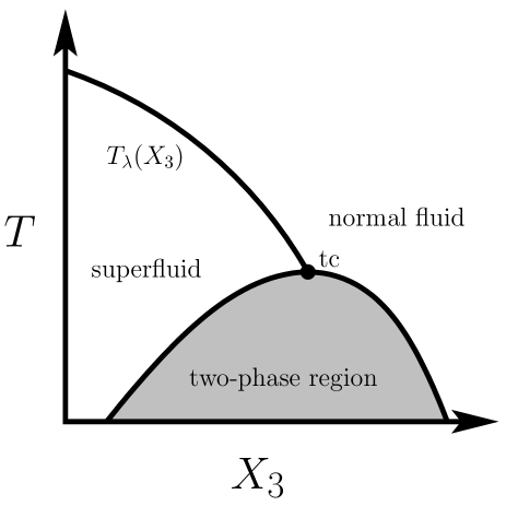
Figure 2: Schematic bulk phase diagram of ${{}^{3}\text{He}}$ -${{}^{4}\text{He}}$ mixtures at fixed pressure. $X_{3}$ is the concentration of ${{}^{3}\text{He}}$ and $T_{\lambda}(X_{3})$ is the line of continuous superfluid transitions, which turn into first-order superfluid transitions at the tricritical point tc. Note that $T_{\lambda}(X_{3})$ meets the two-phase region at its top. If $T_{\lambda}(X_{3})$ would meet the two-phase region below $T_{\text{tc}}$, this would imply that there is either a discontinuous phase transition between two normal fluid phases or between two superfluid phases, which is not the case.

Figure 3: Schematic phase diagram of ${{}^{3}\text{He}}$ -${{}^{4}\text{He}}$ mixtures in the $(T,Z,P)$ space, where $Z=\exp(\mu_{3}/T)$ is the fugacity of ${{}^{3}\text{He}}$ and $P$ is the pressure. $A_{1}$ and $A_{2}$ are the surfaces of the first-order solid-liquid and vapor-liquid phase transitions, respectively, whereas $A_{3}$ and $A_{4}$ are the surfaces of second- and first-order phase transitions between the normal fluid and the superfluid, respectively. A₃ intersects A₁ and A₂ along a line of critical end points connecting ce⁺ with tce⁺ and ce with tce, respectively. The surfaces $A_{3}$ and $A_{4}$ are separated by a line of tricritical points TC which meets $A_{1}$ and $A_{2}$ at the tricritical end points tce⁺ and tce, respectively. $A_{2}$ terminates at a line of critical points, starting from c in the plane $Z=0$. The phase diagram in the plane $Z=0$ is the same as the one in Fig. 1. The dashed lines have no physical meaning; they indicate that the corresponding surface continues. The arrow l_w indicates the thermodynamic path along which tricritical end point wetting occurs.

In order to be able to study wetting films in ${{}^{3}\text{He}}$ -${{}^{4}\text{He}}$ mixtures which have been used to analyze experimentally the tricritical Casimir effect Garcia and Chan (2002), the theoretical description of ${{}^{3}\text{He}}$ -${{}^{4}\text{He}}$ mixtures requires to take into account the occurrence of a vapor phase. Tricritical Casimir forces acting on the liquid-vapor interface of ${{}^{3}\text{He}}$ -${{}^{4}\text{He}}$ wetting films arise due to the confinement of the tricritical fluctuations of the superfluid order parameter and of the composition near the tricritical point of the mixture. The considerable interest in this subject has been triggered both by theoretical predictions Krech and Dietrich (1992a, b) and by experiments in which superfluid wetting films (${{}^{4}\text{He}}$ Garcia and Chan (1999); Ganshin et al. (2006) and ${{}^{3}\text{He}}$ -${{}^{4}\text{He}}$ Garcia and Chan (2002)) were used to provide first reliable evidences for critical Casimir forces. Specifically, concerning tricriticality a ${{}^{3}\text{He}}$ -${{}^{4}\text{He}}$ mixture was prepared in a thermodynamic state of the vapor phase, close to coexistence with the liquid phase. Upon decreasing undersaturation (see the thermodynamic path l_w in Fig. 3), a complete wetting film was grown at the plates of capacitors, the equilibrium thickness of which could be determined very accurately from capacitance measurements. From the balance of the effective forces acting on the depinning liquid-vapor interface such as to thicken or to thinnen the film, the universal scaling function of the tricritical Casimir force was determined.

The, at present, only available corresponding theoretical analysis Maciołek et al. (2007) of the behavior of the tricritical Casimir scaling functions describing the ${{}^{3}\text{He}}$ -${{}^{4}\text{He}}$ wetting film thicknesses, employs the VBEG model without vacancies, and thus does not incorporate the vapor phase. Within this simplified approach, the wetting films have been modeled by a slab geometry with the boundaries introduced by fiat and not of via the actual self-consistent formation as a wetting film. Therefore, it is an open question how the critical Casimir forces emerge in the ${{}^{3}\text{He}}$ -${{}^{4}\text{He}}$ wetting films when the system is brought towards the critical or the tricritical end point, i.e., approaching liquid-vapor coexistence from the vapor side. The present bulk analysis is a prerequisite of such investigations.

The model proposed here is a classical spin-1 model, including the continuous O(2) symmetry of the superfluid order parameter, which does allow for vacant sites and therefore exhibits a vapor phase if the number of vacant sites is sufficiently large. The phase diagrams of this model are obtained within mean-field theory. Since there are three order parameters (i.e., the number densities of ${{}^{3}\text{He}}$ and ${{}^{4}\text{He}}$ as well as the order parameter corresponding to the superfluid transition), the phase diagrams of the proposed model exhibit a rich diversity of topologies. The main difficulty of the present study resides in extracting from a high dimensional parameter space the range of parameters for which the phase diagrams have the topology corresponding to the one of the actual ${{}^{3}\text{He}}$ -${{}^{4}\text{He}}$ mixture. In the next section we introduce the model and continue by obtaining various features of the phase diagram. We close with a summary and conclusions.

II THE MODEL

We consider a three–dimensional (d = 3) simple cubic lattice with lattice spacing $a=1$. The lattice sites $\{i\,|\,i=1,...,\mathcal{N}\}$ are occupied by either ${{}^{3}\text{He}}$ or ${{}^{4}\text{He}}$ or they are unoccupied. The Hamiltonian of this system is

$$\begin{split}\mathcal{H}&=-J_{44}N_{44}-J_{33}N_{33}-J_{34}N_{34}\\ &\quad-\mu_{4}N_{4}-\mu_{3}N_{3}-J_{s}\tilde{N}_{44}-\mathbf{H}\cdot\tilde{\mathbf{N}}_{4}\text{,}\end{split}$$ (1)

where $N_{\text{m}\text{n}}$, with $\text{m},\text{n}\in\{3,4\}$, denotes the number of pairs of nearest neighbors of species m and n on the lattice sites, $N_{\text{m}}$ denotes the number of atoms of species m, and $-J_{s}\tilde{N}_{44}$ denotes the sum of the interaction energy between the superfluid degrees of freedom $\Theta_{i}$ and $\Theta_{j}$ associated with the nearest–neighbor pairs $\langle i,j\rangle$ of ${{}^{4}\text{He}}$ with $J_{s}$ as the corresponding interaction strength. $J_{33}$, $J_{44}$, and $J_{34}$ describe the effective interactions between the three types of pairs of He isotopes. The ${{}^{3}\text{He}}$- ${{}^{3}\text{He}}$ and ${{}^{4}\text{He}}$- ${{}^{4}\text{He}}$ pair potentials between the isotopes are not quite the same due to the slight differences in their electronic states. Moreover, the corresponding effective interactions differ due to the distinct statistics of the two isotopes. The chemical potential of species m is denoted as $\mu_{\text{m}}$. $\mathbf{H}=(H_{x},H_{y})$ is the field conjugate to the superfluid degrees of freedom given by the vector $(\cos\Theta_{i},\sin\Theta_{i})$, provided that the lattice site $i$ is occupied by a ${{}^{4}\text{He}}$ atom.

In order to proceed, we express $N_{\text{m}}$ and $N_{\text{m}\text{n}}$ in terms of occupation numbers of the lattice sites $\{i\}$. We associate with each lattice site $i$ an occupation variable $s_{i}$ which can take the three values $+1$, $-1$, or $0$, where $+1$ means that the lattice site is occupied by ${{}^{4}\text{He}}$, $-1$ means the lattice site is occupied by ${{}^{3}\text{He}}$, and $0$ means the lattice site is unoccupied. Accordingly one has

$$\begin{split}&N_{4}=\frac{1}{2}\sum_{i}s_{i}(s_{i}+1)\equiv\sum_{i}p_{i}\text{,}\\ &N_{3}=\frac{1}{2}\sum_{i}s_{i}(s_{i}-1)\text{,}\\ &N_{44}=\frac{1}{4}\sum_{<i,j>}(s_{i}(s_{i}+1)s_{j}(s_{j}+1))\equiv\sum_{<i,j>}p_{i}p_{j}\text{,}\\ &N_{33}=\frac{1}{4}\sum_{<i,j>}(s_{i}(s_{i}-1)s_{j}(s_{j}-1))\text{,}\\ &N_{34}=\frac{1}{4}\sum_{<i,j>}(s_{i}(s_{i}+1)s_{j}(s_{j}-1)+s_{i}(s_{i}-1)s_{j}(s_{j}+1))\text{,}\end{split}$$ (2)

where $\sum\limits_{<i,j>}$ denotes the sum over nearest neighbors. Using the above definitions one obtains

$$\begin{split}\mathcal{H}&=-K\sum_{<i,j>}s_{i}s_{j}-J\sum_{<i,j>}q_{i}q_{j}-C\sum_{<i,j>}(s_{i}q_{j}+q_{i}s_{j})\\ &\quad-\Delta_{-}\sum_{i}s_{i}-\Delta_{+}\sum_{i}q_{i}-J_{s}\sum_{<i,j>}p_{i}p_{j}\cos(\Theta_{i}-\Theta_{j})\\ &\quad-H_{x}\sum_{i}p_{i}\cos\Theta_{i}-H_{y}\sum_{i}p_{i}\sin\Theta_{i}\text{,}\end{split}$$ (3)

where

$$\begin{split}&\sum_{<i,j>}p_{i}p_{j}\cos(\Theta_{i}-\Theta_{j})=\tilde{N}_{44}=\sum_{<i,j>}p_{i}p_{j}\begin{pmatrix}\cos\Theta_{i}\\ \sin\Theta_{i}\end{pmatrix}\cdot\begin{pmatrix}\cos\Theta_{j}\\ \sin\Theta_{j}\end{pmatrix},\\ &\sum_{i}p_{i}(\cos\Theta_{i},\sin\Theta_{i})=\tilde{\mathbf{N}}_{4},\end{split}$$ (4)

and

$$\begin{split}&q_{i}=s_{i}^{2}\text{,}\\ &p_{i}=\frac{1}{2}s_{i}(s_{i}+1)\text{,}\\ &K=\frac{1}{4}(J_{44}+J_{33}-2J_{34})\text{,}\\ &J=\frac{1}{4}(J_{44}+J_{33}+2J_{34})\text{,}\\ &C=\frac{1}{4}(J_{44}-J_{33})\text{,}\\ &\Delta_{-}=\frac{1}{2}(\mu_{4}-\mu_{3})\text{,}\\ &\Delta_{+}=\frac{1}{2}(\mu_{4}+\mu_{3})\text{,}\end{split}$$ (5)

and $\Theta_{i}\in[0,2\pi]$ represents the superfluid degree of freedom at the lattice site i, provided it is occupied by ${{}^{4}\text{He}}$.

III MEAN-FIELD THEORY

In this section we apply mean-field theory to the above model. This approximation follows from a variational method based upon approximating the total equilibrium density matrix by a product of density matrices associated with each lattice site Chaikin and Lubensky (1995).

Due to the variation principle, the free energy $F$ obeys the following inequality:

$$F\leq\phi=\hat{T}r(\rho\mathcal{H})+(1/\beta)\hat{T}r(\rho\ln\rho)\text{,}$$ (6)

where $\rho$ is any trial density matrix with $\hat{T}r(\rho)=1$, with respect to which $\phi$ on the rhs of Eq. (6) should be minimized in order to obtain the best approximation;

$$\hat{T}r=\sum_{s_{1}=\pm 1,0}\int_{0}^{2\pi}\text{d}\Theta_{1}\cdot...\cdot\sum_{s_{\mathcal{N}}=\pm 1,0}\int_{0}^{2\pi}\text{d}\Theta_{\mathcal{N}}$$ (7)

denotes the trace and $\beta=1/T$ where $T$ is the temperature times $k_{\text{B}}$. The mean-field approximation assumes that any lattice site experiences the same mean field generated by its neighborhood so that the total density matrix will be the product of the density matrices corresponding to each lattice site:

$$\rho=\prod_{i}\rho_{i},$$ (8)

with

$$Tr\rho_{i}=\sum_{s_{i}=\pm 1,0}\int_{0}^{2\pi}\text{d}\Theta_{i}\rho_{i}(s_{i},\Theta_{i})=1.$$ (9)

For homogeneous bulk systems the local density matrix is independent of the site.

The variational mean-field free energy per site for the Hamiltonian introduced in the previous section is (with $\cos(\Theta_{i}-\Theta_{j})=\cos\Theta_{i}\cos\Theta_{j}+\sin\Theta_{i}\sin\Theta_{j}$)

$$\begin{split}\frac{\phi}{\mathcal{N}}&=-\frac{z}{2}[K\langle s_{i}\rangle^{2}+J\langle q_{i}\rangle^{2}+2C\langle q_{i}\rangle\langle s_{i}\rangle\\ &\quad+J_{s}(\langle p_{i}\cos\Theta_{i}\rangle^{2}+\langle p_{i}\sin\Theta_{i}\rangle^{2})]\\ &\quad-\Delta_{-}\langle s_{i}\rangle-\Delta_{+}\langle q_{i}\rangle-H_{x}\langle p_{i}\cos\Theta_{i}\rangle-H_{y}\langle p_{i}\sin\Theta_{i}\rangle\\ &\quad+(1/\beta)Tr(\rho_{i}\ln\rho_{i})\text{,}\end{split}$$ (10)

where $\mathcal{N}$ is the total number of sites and $z$ is the coordination number of the lattice ($z=2d$, where $d$ is the spatial dimension of the system; here $z=6$), and $\langle...\rangle=Tr(\rho_{i}...)$ denotes the thermal average, taken with the trial density matrix $\rho_{i}$ associated with the lattice site i.

Minimizing the variational function $\phi/\mathcal{N}$ with respect to $\rho_{i}$ renders the best normalized functional form of $\rho_{i}$. There are two approaches to find the variational minima. In the first approach one parametrizes the density matrix $\rho_{i}$ in terms of the order parameters of the phase transitions and minimizes $\phi/\mathcal{N}$ with respect to the coefficients multiplying these order parameters. In the second approach one treats $\rho$ itself as a variational function and minimizes $\phi/\mathcal{N}$ with respect to it Chaikin and Lubensky (1995). We follow the second approach and calculate the functional derivative of $\phi/\mathcal{N}$ in Eq. (10) with respect to $\rho_{i}(s_{i},\Theta_{i})$ using $\frac{\delta\rho_{i}(s_{i},\Theta_{i})}{\delta\rho_{j}(s_{j},\Theta_{j})}=\delta(\Theta_{i}-\Theta_{j})\delta_{s_{i},s_{j}}$, and equate it to the Lagrange multiplier $\eta$ corresponding to the constraint $Tr(\rho_{i})=1$

$$\begin{split}\eta&=\frac{\delta(\phi/\mathcal{N})}{\delta\rho_{i}(s_{i},\Theta_{i})}\\ &=-z[K\langle s_{i}\rangle s_{i}+J\langle q_{i}\rangle q_{i}+C(q_{i}\langle s_{i}\rangle+\langle q_{i}\rangle s_{i})\\ &\quad+J_{s}(\langle p_{i}\cos\Theta_{i}\rangle p_{i}\cos\Theta_{i}+\langle p_{i}\sin\Theta_{i}\rangle p_{i}\sin\Theta_{i})]\\ &\quad-\Delta_{-}s_{i}-\Delta_{+}q_{i}-H_{x}p_{i}\cos\Theta_{i}-H_{y}p_{i}\sin\Theta_{i}\\ &\quad+(1+\ln\rho_{i})/\beta\text{.}\end{split}$$ (11)

Equation (11) can be solved for $\rho_{i}(s_{i},\Theta_{i})$:

$$\rho_{i}=e^{\beta\eta-1-\beta h_{i}}\text{,}$$ (12)

where

$$\begin{split}h_{i}(s_{i},\Theta_{i})=&-s_{i}(kX+cD+\Delta_{-})-q_{i}(jD+cX+\Delta_{+})\\ &-p_{i}((j_{s}M_{x}+H_{x})\cos\Theta_{i}+(j_{s}M_{y}+H_{y})\sin\Theta_{i})\end{split}$$ (13)

is the single-site Hamiltonian in which the coupling constants are rescaled as $j=zJ$, $c=zC$, $k=zK$, $j_{s}=zJ_{s}$ and where the following order parameters are introduced:

$$\begin{split}&X:=\langle s_{i}\rangle\text{,}\\ &D:=\langle q_{i}\rangle\text{,}\\ &M_{x}:=\langle p_{i}\cos\Theta_{i}\rangle\text{,}\\ &M_{y}:=\langle p_{i}\sin\Theta_{i}\rangle\text{,}\end{split}$$ (14)

which in the bulk are independent of $i$. In accordance with Eq. (4) one has $\langle\tilde{\mathbf{N}}_{4}\rangle=\mathcal{N}\mathbf{M}$. The normalization $Tr(\rho_{i})=1$ yields

$$e^{-\beta\eta+1}=Tr(e^{-\beta h_{i}})$$ (15)

so that

$$\rho_{i}=\frac{e^{-\beta h_{i}}}{Tr(e^{-\beta h_{i}})}\text{,}$$ (16)

where $h_{i}$ is given by Eq. (13).

The order parameters defined in Eq. (14) allow one to determine the number densities $X_{4}=\frac{\langle N_{4}\rangle}{\mathcal{N}}=\frac{D+X}{2}$ and $X_{3}=\frac{\langle N_{3}\rangle}{\mathcal{N}}=\frac{D-X}{2}$ so that $X=(\langle N_{4}\rangle-\langle N_{3}\rangle)/\mathcal{N}=X_{4}-X_{3}$ is the difference of the number densities and $D=(\langle N_{4}\rangle+\langle N_{3}\rangle)/\mathcal{N}$ is the total number density. The concentration of ${{}^{4}\text{He}}$ and ${{}^{3}\text{He}}$ is $\frac{\langle N_{4}\rangle}{\langle N_{4}\rangle+\langle N_{3}\rangle}\equiv\mathcal{C}_{4}=\frac{D+X}{2D}=X_{4}/D$ and $\frac{\langle N_{3}\rangle}{\langle N_{4}\rangle+\langle N_{3}\rangle}\equiv\mathcal{C}_{3}=\frac{D-X}{2D}=X_{3}/D$, respectively. $M_{x}$ and $M_{y}$ are the components of the two-dimensional superfluid order parameter $\mathbf{M}=(M_{x},M_{y})$ with $M:=\sqrt{|\mathbf{M}|^{2}}=\sqrt{M_{x}^{2}+M_{y}^{2}}$. The equilibrium superfluid order parameter $\mathbf{M}$ points into the direction of $\mathbf{H}$. This follows from the principle of minimum free energy together with the relation $\frac{\partial F}{\partial\mathbf{H}}=-\mathbf{M}$, where $F$ is the free energy of the system, which implies that for fixed $T$, $\Delta_{+}$, and $\Delta_{-}$ one has $\text{d}F=-\text{d}\mathbf{H}\cdot\mathbf{M}$. Thus for $\mathbf{H}$ with an orientation $\psi$, i.e., $\mathbf{H}=(H_{x},H_{y})=H(\cos\psi,\sin\psi)$ with $H:=\sqrt{|\mathbf{H}|^{2}}=\sqrt{H_{x}^{2}+H_{y}^{2}}$, $\mathbf{M}$ points into the same direction, i.e., $\mathbf{M}=(M_{x},M_{y})=M(\cos\psi,\sin\psi)$.
Within the aforementioned mean field approximation the order parameters $X(\Delta_{-},\Delta_{+},H,T)=Tr(\rho_{i}s_{i})$, $D(\Delta_{-},\Delta_{+},H,T)=Tr(\rho_{i}q_{i})$, and $M(\Delta_{-},\Delta_{+},H,T)$ (with the latter obtained from $M_{x}=Tr(\rho_{i}p_{i}\cos\Theta_{i})$ and $M_{y}=Tr(\rho_{i}p_{i}\sin\Theta_{i})$) are given by three coupled self-consistent equations:

$$X=\frac{-W(X,D;\Delta_{-},\Delta_{+},H,T)+R(X,D;\Delta_{-},\Delta_{+},H,T)I_{0}(\beta j_{s}M+\beta H)}{1+W(X,D;\Delta_{-},\Delta_{+},H,T)+R(X,D;\Delta_{-},\Delta_{+},H,T)I_{0}(\beta j_{s}M+\beta H)}\text{,}$$ (17)

$$D=\frac{W(X,D;\Delta_{-},\Delta_{+},H,T)+R(X,D;\Delta_{-},\Delta_{+},H,T)I_{0}(\beta j_{s}M+\beta H)}{1+W(X,D;\Delta_{-},\Delta_{+},H,T)+R(X,D;\Delta_{-},\Delta_{+},H,T)I_{0}(\beta j_{s}M+\beta H)}\text{,}$$ (18)

and

$$M=\frac{R(X,D;\Delta_{-},\Delta_{+},H,T)I_{1}(\beta j_{s}M+\beta H)}{1+W(X,D;\Delta_{-},\Delta_{+},H,T)+R(X,D;\Delta_{-},\Delta_{+},H,T)I_{0}(\beta j_{s}M+\beta H)}\text{,}$$ (19)

where $I_{0}$ and $I_{1}$ are modified Bessel functions (see Sec. 9.6 in Ref. Abramowitz and Stegun (1972)). The functions $W(X,D;\Delta_{-},\Delta_{+},H,T)$ and $R(X,D;\Delta_{-},\Delta_{+},H,T)$ are given by

$$W(X,D;\Delta_{-},\Delta_{+},H,T)=e^{\beta[(c-k)X+(j-c)D+\Delta_{+}-\Delta_{-}]}>0$$ (20)

and

$$R(X,D;\Delta_{-},\Delta_{+},H,T)=e^{\beta[(c+k)X+(j+c)D+\Delta_{+}+\Delta_{-}]}>0$$ (21)

so that $D>X$. The equilibrium free energy $\phi(\Delta_{-},\Delta_{+},H,T)$ is given by

$$\begin{split}\phi(\Delta_{-},\Delta_{+},H,T)=&\frac{k}{2}X^{2}+\frac{j}{2}D^{2}+cXD+\frac{j_{s}}{2}M^{2}\\ &+\frac{1}{\beta}\ln(1-D)\text{.}\end{split}$$ (22)

In the limit $\Delta_{+}\rightarrow+\infty$ both $W$ and $R$ diverge so that according to Eq. (18) one has $D(\Delta_{-},\Delta_{+}\rightarrow+\infty,H,T)\rightarrow 1$, i.e., all lattice sites are occupied and the concentrations reduces to $\mathcal{C}_{4}=(1+X)/2$ and $\mathcal{C}_{3}=(1-X)/2$. With the explicit expressions in Eqs. (20) and (21), in the limit $\Delta_{+}\rightarrow+\infty$, Eqs. (17) and (19), reduce to:

$$X=\frac{-e^{-\beta(2kX+2c+2\Delta_{-})}+I_{0}(\beta j_{s}M+\beta H)}{e^{-\beta(2kX+2c+2\Delta_{-})}+I_{0}(\beta j_{s}M+\beta H)},\qquad\Delta_{+}=\infty,$$ (23)

and

$$M=\frac{I_{1}(\beta j_{s}M+\beta H)}{e^{-\beta(2kX+2c+2\Delta_{-})}+I_{0}(\beta j_{s}M+\beta H)},\qquad\Delta_{+}=\infty\text{.}$$ (24)

Expressing $X$ in Eqs. (23) and (24) in terms of $\mathcal{C}_{4}$ renders

$$\mathcal{C}_{4}=\frac{I_{0}(\beta j_{s}M+\beta H)}{e^{\beta(-\tilde{k}\mathcal{C}_{4}+\tilde{\Delta}_{-})}+I_{0}(\beta j_{s}M+\beta H)},\qquad\Delta_{+}=\infty\text{,}$$ (25)

and

$$M=\frac{I_{1}(\beta j_{s}M+\beta H)}{e^{\beta(-\tilde{k}\mathcal{C}_{4}+\tilde{\Delta}_{-})}+I_{0}(\beta j_{s}M+\beta H)},\qquad\Delta_{+}=\infty\text{,}$$ (26)

where $\tilde{k}=4k$ and $\tilde{\Delta}_{-}=2(-\Delta_{-}+k-c)$. For $H=0$ these equations have the same form as the corresponding ones in Ref. Maciołek et al. (2004), which do not allow for vacant sites from outset. Thus in the limit $\Delta_{+}\rightarrow+\infty$ and for $H=0$ our present more general results reduce to those of the more restricted model studied before.

IV PHASE DIAGRAM

In this section we determine the phase diagram of the VBEG model within mean-field theory. Although certain features of the phase diagram can be obtained analytically, most parts of it can be determined only numerically. In order to find the coexisting states of phase equilibria, one has to identify those distinct states $(X_{\nu},D_{\nu},M_{\nu})$, which share the same values for the chemical potentials and the pressure at a common temperature. The chemical potentials can be obtained by solving Eqs. (17) and (18) together with Eqs. (20) and  (21) for $\Delta_{+}$ and $\Delta_{-}$:

$$\begin{split}\Delta_{+}(X,D,M;H,T)\,=\,\,&\,\frac{T}{2}\ln(D^{2}-X^{2})-T\ln(2(1-D))-cX-jD\\ &\,-\frac{T}{2}\ln(I_{0}(j_{s}M/T+H/T))\end{split}$$ (27)

and

$$\Delta_{-}(X,D,M;H,T)\,=\,\,\frac{T}{2}\ln\frac{D+X}{D-X}-kX-cD-\frac{T}{2}\ln(I_{0}(j_{s}M/T+H/T))\text{.}$$ (28)

Within the grand canonical ensemble the pressure is given by $\phi/\mathcal{N}=-P$. (Note that the sample volume is $V=\mathcal{N}a^{3}$, here with $a=1$). According to Eqs. (17) - (19) the order parameters of any state must fulfill the relation

$$\frac{2M}{X+D}=\frac{M}{X_{4}}=\frac{I_{1}(\beta j_{s}M+\beta H)}{I_{0}(\beta j_{s}M+\beta H)}\text{,}$$ (29)

which expresses $M$ in terms of $\frac{X+D}{2}=X_{4}$, $T$, and $H$. Depending on the value of the coupling constant $j_{s}$ the phase diagram exhibits various topologies.

IV.1 Phase diagram for a simple, normal liquid mixture: $j_{s}=0$

For $j_{s}=0$ and $H=0$ there is no superfluid phase and $M$ is always zero (compare Eq. (29) with $I_{1}(y\rightarrow 0)=\frac{1}{2}y$ and $I_{0}(y\rightarrow 0)=1$). For $j_{s}=0$, due to $I_{0}(0)=1$ the last term in Eq. (27) and in Eq. (28) drops out. Thus the phase diagram will be that of a simple binary normal liquid mixture of species 3 and 4, similar to the ones shown in Refs. Sivardière and Lajzerowicz (1975); Dietrich and Latz (1989); Getta and Dietrich (1993). The first-order demixing transitions occur at low temperatures, whereas at high temperatures the liquid is mixed. The demixing transitions terminate in a line of critical points which due to $\frac{{\partial}\phi}{{\partial}X}=-\Delta_{-}$ (see Eqs. (10) and (14)) are given by Chaikin and Lubensky (1995)

$$\frac{\mathrm{d}\Delta_{-}}{\mathrm{d}X}|_{\Delta_{+},T}=\frac{\mathrm{d}^{2}\Delta_{-}}{\mathrm{d}X^{2}}|_{\Delta_{+},T}=0\text{,}\quad\frac{\mathrm{d}^{3}\Delta_{-}}{\mathrm{d}X^{3}}|_{\Delta_{+},T}>0\text{,}$$ (30)

where $\frac{\mathrm{d^{\text{n}}}\Delta_{-}}{\mathrm{d}X^{\text{n}}}|_{\Delta_{+},T}$ denotes the $\text{n}^{\text{th}}$ total derivative of $\Delta_{-}$ (see Eq. (28)) with respect to $X$ at constant $\Delta_{+}$ and $T$. Note that the independent variables are $(T,\Delta_{+},\Delta_{-})$. Since $\Delta_{-}$ as given by Eq. (28) depends on $D$, which for $\Delta_{+}=const$ depends in turn implicitly on $X$ via Eq. (27), calculating the total derivative of $\Delta_{-}$ with respect to $X$ requires the knowledge of the partial derivative of $D$ with respect to $X$. Thus the first condition in Eq. (30) reads

$$\frac{\mathrm{d}\Delta_{-}}{\mathrm{d}X}|_{\Delta_{+},T}=\frac{\mathrm{\partial}\Delta_{-}}{\mathrm{\partial}X}|_{\Delta_{+},T}+\frac{\mathrm{\partial}\Delta_{-}}{\mathrm{\partial}D}\frac{\mathrm{\partial}D}{\mathrm{\partial}X}|_{\Delta_{+},T}=0\text{,}$$ (31)

where $\frac{\partial\Delta_{-}}{\partial X}$ and $\frac{\partial\Delta_{-}}{\partial D}$ follow from Eq. (28) and where $\frac{\mathrm{\partial}D}{\mathrm{\partial}X}|_{\Delta_{+},T}$ is obtained by taking the derivative of Eq. (27) with respect to $X$ at fixed $\Delta_{+}$ and $T$ and by solving for $\frac{\mathrm{\partial}D}{\mathrm{\partial}X}|_{\Delta_{+},T}$. Accordingly, the first condition in Eq. (30) leads to a quadratic equation:

$$T^{2}+a_{1}T+a_{0}=0$$ (32)

with

$$\begin{split}&a_{1}=-D(-2cX+j+k)+X(kX-2c)+D^{2}j\text{,}\\ &a_{0}=(D-1)(D^{2}-X^{2})\left(c^{2}-jk\right).\end{split}$$ (33)

Equation (32) renders as solution two branches $T_{1,2}(X,D)$. Similarly, the second condition in Eq. (30) leads to an equation $G(X,D,T)=0$ where, due to the first condition, $T=T_{1,2}(X,D)$. Thus it takes the form $G(X,D,T_{1,2}(X,D))=:g_{1,2}(X,D)=0$. Therefore, for a given value $D^{(0)}$ of $D$, the solution of $g_{1,2}(X,D^{(0)})=0$ (which must be solved numerically) renders $X(D_{1,2}^{(0)})=X_{1,2}^{(0)}$ so that at $T_{1,2}^{(0)}=T_{1,2}(X_{1,2}^{(0)},D_{1,2}^{(0)})$ the model exhibits a critical point, provided the condition $\frac{\mathrm{d}^{3}\Delta_{-}}{\mathrm{d}X^{3}}|_{\Delta_{+},T}>0$ is fulfilled. This latter condition and the physical constraints $T>0$, $P>0$, and $D>|X|$ exclude one of the two branches of $T_{1,2}(X,D)$. Thus for various values of $D$ one obtains a set of points $\{(D,X(D),T(X(D),D))\}$, which forms a line of critical points in the space spanned by $(X,D,T)$. According to Eqs. (27) and (28), the set $\{(D,X,T)\}$ can be transformed to the set $\{(\Delta_{+}(D,X;T),\Delta_{-}(D,X;T),T)\}$, which yields a line of critical points in the space spanned by $(\Delta_{+},\Delta_{-},T)$. This line ends at the liquid-vapor coexistence surface forming a critical end point (see Fig. 4).

Figure 4: The schematic phase diagram for $H=0$ and $j_{s}=0$ (i. e., without coupling between the superfluid degrees of freedom). The phase diagram in the plane $Z=0$ is that of a one-component system consisting of particles "4". Upon increasing the fugacity $Z$ of particles "3", the transition lines in the plane $Z=0$ extend to form three distinct surfaces. The surface SL is a surface of first-order phase transitions between the solid and the liquid phases. The transition surfaces between the vapor and the liquid phases, and between the solid and the liquid phases are denoted by VL and SV, respectively. The surface VL terminates at a line of critical points (green line). The critical point of the pure system of "4" particles is denoted by ’e’. The liquid can be either mixed or demixed. Concerning the demixed phases, LL denotes the surface of first-order phase transitions between the phase rich in component 3 (large $Z$) and the phase rich in the component 4 (small $Z$). This surface terminates at a line of critical points (brown line), which meets the surfaces SL and VL at the critical end points ’b’ and ’c’, respectively. The point ’a’ is a quadruple point, whereas ’d’ is a triple point. The lines a-b, a-c, and a-d are triple lines. The dashed lines have no physical meaning; they indicate that the corresponding surfaces continue.

Figure 5: Phase diagrams for the coupling constants $(c/k,j/k,j_{s}/k)=(1,5.714,0)$ and $H=0$. Along the triple line of three-phase coexistence (see line a-c in Fig. 4) the figures show the first-order demixing transitions of the liquid at coexistence with the vapor phase (a) in the $(X^{l}_{3}$, $T)$ plane, with $X^{l}_{3}=\langle N_{3}\rangle_{l}/\mathcal{N}$ corresponding to the 3-particles in the liquid phase, (b) in the $(X_{v}$, $T)$ plane at coexistence with the two liquid phases, where $X_{v}=(\langle N_{4}\rangle_{v}-\langle N_{3}\rangle_{v})/\mathcal{N}$ in the vapor phase, (c) in the $(D_{l}$, $T)$ plane, where $D_{l}=(\langle N_{4}\rangle_{l}+\langle N_{3}\rangle_{l})/\mathcal{N}$ in the liquid phase, and (d) in the $(D_{v}$, $T)$ plane, where $D_{v}=(\langle N_{4}\rangle_{v}+\langle N_{3}\rangle_{v})/\mathcal{N}$ in the vapor phase. The indices ’$l$’ and ’$v$’ refer to the values of the order parameters in the liquid and in the vapor phase, respectively. The critical end point ce here corresponds to the point c in Fig. 4. Panels (e) and (f) show the dependences of the pressure $P$ and of the fugacity $Z=\exp(\mu_{3}/T)$ on the temperature along the triple line a-c in Fig. 4. The two liquid states become identical at the critical end point ce at $T_{\text{ce}}/k=1.947$, above which the liquid is mixed. The coexisting liquid and vapor phases at ce are $(X^{\text{ce}}_{l},D^{\text{ce}}_{l},M^{\text{ce}}_{l})=(0.050,0.913,0)$ and $(X^{\text{ce}}_{v},D^{\text{ce}}_{v},M^{\text{ce}}_{v})=(-0.120,0.180,0)$, respectively. The transitions between the vapor phase and the liquid phases are always first order. According to (e) and (f), along a-c both $P$ and $Z$ vary as function of $T$, with the requirement of staying in coexistence with the vapor phase. This implies that the white domains in (a) and (c) are not projections of a three-dimensional surface, given by the equation of state, onto the $(T,X_{3})$ and $(T,D)$ plane, respectively. The black lines provide only the $T$-dependence of $X_{3}$ and $D_{l}$ along the line a-c, which contains two branches. Similar remarks hold for Figs. 9-12.

The schematic phase diagram for $j_{s}=0$ in the $(T,Z,P)$ space is shown in Fig. 4, with $Z=\exp(\mu_{3}/T)$. There are four surfaces separating various phases: the surface SL of first-order phase transitions between the solid and the liquid phases, the surface VL of first-order phase transitions between the vapor and the liquid phases, the surface SV of first-order phase transitions between the solid and the liquid phases, and the surface LL of first-order phase transitions between the phase rich in component 3 and the phase rich in the component 4. This latter surface terminates at a line of critical points (brown line), and VL terminates at a line of critical points (green line).

In Fig. 5, the demixing transitions at coexistence with the vapor phase (see the line connecting the points ’a’ and ’c’ in Fig. 4) are shown for the coupling constants chosen as $(c/k,j/k,j_{s}/k)=(1,5.714,0)$. Along this triple line of first-order liquid-liquid transitions at coexistence with the vapor phase, three thermodynamic states with distinct number densities and concentrations coexist. The values of the order parameters of these three states are shown in Figs. 5(a)-(d). The corresponding values of the pressure $P/k$ and of the fugacity, $Z=\exp(\mu_{3}/T)=\exp(\frac{\mu_{3}}{k}\frac{1}{T/k})$ of the component 3 of the mixture ($\mu_{3}=\Delta_{+}-\Delta_{-}$ and $T$ are rescaled by the coupling constant $k$) are shown in Figs. 5(e) and (f), respectively. The vapor phase is characterized by a small value $D_{v}$ of the order parameter $D$, whereas a large value $D_{l}$ of the density order parameter $D$ corresponds to the liquid state. In Fig. 5, at fixed temperatures below the critical end point (ce) (which is denoted as ’c’ in Fig. 4), three values for $X_{3}$, i.e., two values $X_{3}^{l}$ for $X_{3}$ in the liquid phases (Fig. 5(a)) and one value for the vapor phase ($X_{v}$ in Fig. 5(b)), and three values for $D$ (Figs. 5 (c)-(d)) characterize the three states which share the same values of the pressure (Fig. 5(e)) and of the chemical potentials (and thus the fugacity, Fig. 5(f)). At $T_{\text{ce}}/k=1.947$ the two liquid states merge into a single state with $(X^{\text{ce}}_{l},D^{\text{ce}}_{l},M^{\text{ce}}_{l})=(0.050,0.913,0)$, which coexists with the vapor state characterized by $(X^{\text{ce}}_{v},D^{\text{ce}}_{v},M^{\text{ce}}_{v})=(-0.120,0.180,0)$. For $T>T_{\text{ce}}$ the liquid is mixed. The transitions between the vapor and the liquid phases are always first order, above and below $T_{\text{ce}}$.

IV.2 Phase diagram including the superfluid phase: $j_{s}>0$

For $j_{s}>0$ the model exhibits superfluid transitions, which can be either first or second order. In order to find the surface of second-order phase transitions to the superfluid phase (see A₃ in Fig. 3), we introduce the appropriate thermodynamic potential $A$ as the Legendre transform of $\phi$:

$$A(\Delta_{-},\Delta_{+},M,T)=\phi(\Delta_{-},\Delta_{+},H(\Delta_{-},\Delta_{+},M,T),T)-MH(\Delta_{-},\Delta_{+},M,T)\text{,}$$ (34)

where, according to Eq. (1), $\frac{\partial\phi(\Delta_{-},\Delta_{+},M,T)}{\partial H}=M$ which implicitly renders $H=H(\Delta_{-},\Delta_{+},M,T)$ so that $\frac{\partial A(\Delta_{-},\Delta_{+},M,T)}{\partial M}=-H(\Delta_{-},\Delta_{+},M,T)$. In order to determine $H(\Delta_{-},\Delta_{+},M,T)$ we use Eq. (29). Because we are interested in the phase diagram for $H=0$, we replace the right hand side of Eq. (29) by its approximation linear in $H$:

$$\frac{2M}{X+D}=\frac{I_{1}\left(j_{s}M/T\right)}{I_{0}\left(j_{s}M/T\right)}+\frac{H}{T}\frac{I_{1}^{{}^{\prime}}\left(j_{s}M/T\right)I_{0}\left(j_{s}M/T\right)-I_{0}^{{}^{\prime}}\left(j_{s}M/T\right)I_{1}\left(j_{s}M/T\right)}{I_{0}^{2}\left(j_{s}M/T\right)}.$$ (35)

Solving this equation for $H$ (using $I_{0}^{{}^{\prime}}=I_{1}$, $I_{1}^{{}^{\prime}}=(I_{0}+I_{2})/2$, and $I_{2}(a)=I_{0}(a)-\frac{2}{a}I_{1}(a)$) leads to

$$\begin{split}H&=\frac{I_{1}(j_{s}M/T)}{M/T}\frac{2MI_{0}(j_{s}M/T)-(X+D)I_{1}(j_{s}M/T)}{I_{0}^{2}(j_{s}M/T)+I_{0}(j_{s}M/T)I_{2}(j_{s}M/T)-2I_{1}^{2}(j_{s}M/T)}\\ &=\frac{-j_{s}TI_{1}(j_{s}M/T)[-2MI_{0}(j_{s}M/T)+(D+X)I_{1}(j_{s}M/T)]}{2[-j_{s}M(I_{1}(j_{s}M/T))^{2}+I_{0}(j_{s}M/T)[TI_{1}(j_{s}M/T)+j_{s}MI_{2}(j_{s}M/T)]]}.\end{split}$$ (36)

Due to $\frac{\partial A}{\partial M}=-H$ the conditions for the critical points, where $M$ vanishes continuously (see $\text{A}_{3}$ in Fig. 3), are (compare Eq. (30))

$$\frac{dH}{dM}|_{\Delta_{+},\Delta_{-},T}=\frac{d^{2}H}{dM^{2}}|_{\Delta_{+},\Delta_{-},T}=0\text{, }\quad\frac{d^{3}H}{dM^{3}}|_{\Delta_{+},\Delta_{-},T}>0\text{,}$$ (37)

with all total derivatives to be taken at $M=0$ and at constant $\Delta_{+}$, $\Delta_{-}$, and $T$ (compare Eq. (31)). Note that the independent variables are $(T,\Delta_{+},\Delta_{-})$. According to Eq. (36), calculating the total derivatives of $H$ with respect to $M$ requires the expression for $\frac{\partial H}{\partial M}$ and the knowledge of the partial derivatives of $X$ and $D$ with respect to $M$. These latter ones are obtained by taking the partial derivatives of Eqs. (27) and (28) with respect to $M$ at fixed $\Delta_{+}$ and $\Delta_{-}$ and by solving the resulting two coupled equations for the required derivatives $\frac{\partial X}{\partial M}$ and $\frac{\partial D}{\partial M}$.

Applying the conditions for critical points (Eq. (37)) leads to the following expression for the surface $\text{A}_{3}$ of superfluid transitions:

$$T_{s}=\frac{j_{s}}{4}(D+X)\text{.}$$ (38)

We note that the same relation follows independently from Eq. (29) for $H=0$ in the limit $M\rightarrow 0$. The route via Eq. (36) has, however, the additional advantage of facilitating also the calculation of tricritical points (see Eqs. (39)-(41)). Furthermore, expanding the right hand side of Eq. (29) up to and including the order $H^{3}$ leaves the result in Eq. (38) unchanged.

With $D$ and $X$ given by Eqs. (17)-(19) in terms of $\Delta_{+}$, $\Delta_{-}$, and $T$ (note that $H=0$ and that on this surface $M=0$), Eq. (38) renders $T_{s}(\Delta_{-},\Delta_{+})$ which corresponds to a surface in the space spanned by $(\Delta_{+},\Delta_{-},T)$.

This surface of second-order phase transitions between the normal fluid $(M=0)$ and the superfluid $(M\neq 0)$ ends at the surface of liquid-vapor coexistence, forming a line of critical end points (see the line connecting ce and tce in Fig. 3). The conditions for tricritical points are

$$\frac{dH}{dM}|_{\Delta_{+},\Delta_{-},T}=\frac{d^{2}H}{dM^{2}}|_{\Delta_{+},\Delta_{-},T}=\frac{d^{3}H}{dM^{3}}|_{\Delta_{+},\Delta_{-},T}=\frac{d^{4}H}{dM^{4}}|_{\Delta_{+},\Delta_{-},T}=0\text{, }\frac{d^{5}H}{dM^{5}}|_{\Delta_{+},\Delta_{-},T}>0\text{,}$$ (39)

with all total derivatives to be taken also at $M=0$, which again requires to consider the partial derivatives of $X$ and $D$ with respect to $M$, as discussed after Eq. (37). The vanishing of the first four derivatives leads to a quadratic equation for $D$ (where Eq. (38) has been used to eliminate the dependence on $T$):

$$b_{2}D^{2}+b_{1}D+b_{0}=0\text{,}$$ (40)

where the coefficients $b_{0,1,2}$ are given in terms of the order parameter $X$ and the coupling constants:

$$\begin{split}&b_{0}=X(16c^{2}-(4j+j_{s})(4k+j_{s}))\\ &\quad\quad+X^{2}j_{s}(4k+j_{s})\text{,}\\ &b_{1}=2X(j_{s}^{2}-8c^{2}+8jk+2j_{s}(j+k))\\ &\quad\quad-(4c+j_{s})^{2}+16jk\text{,}\\ &b_{2}=16c^{2}+j_{s}(8c-4k+j_{s})-16jk\text{.}\end{split}$$ (41)

We note that, also here, expanding the right hand side of Eq. (29) up to and including the order $H^{2}$ does not change the results in Eqs. (40)-(41).

Accordingly, the solution of Eq. (40) yields $D=D_{0}(X)$ which due to Eqs. (17)-(19) leads to the relation $D(\Delta_{-},\Delta_{+},T)=D_{0}(X(\Delta_{-},\Delta_{+},T))$. This turns into a relationship $T(\Delta_{-},\Delta_{+})$ which corresponds to a surface in the space spanned by $(\Delta_{+},\Delta_{-},T)$. Simultaneously Eq. (38) has to hold which also corresponds to a surface in this space. Thus the tricritical points correspond to the intersection of these two surfaces and thus form a line of tricritical points (TC in Fig. 3). The condition for the fifth derivative along this line can be checked only numerically. This condition and the fact that $D>|X|$ exclude one of the two solutions of Eq. (40). For small values of $j_{s}$ the model exhibits a superfluid transition in the liquid phase (see Fig. 6). In certain parts of the phase diagram this transition is second order, in other parts it is first order. Thus upon switching on $j_{s}$ a new surface LL₃ raises above the bottom (i. e., VL) of the phase diagram shown in Fig. 4 and changes the character of the lower part of the surface LL in Fig. 4, indicated as LL₁, in Fig. 6.
The surface LL₃ of continuous transitions separates the superfluid and the normal fluid both 4-rich. The surface LL₁ corresponds to first-order phase transitions between the 4-rich superfluid and the 3-rich normal fluid. The surface LL₁ $\cup$ LL₂ terminates LL₃ at a line f-i of critical end points.

Figure 6: Schematic phase diagram for small values of $j_{s}$. SL, VL, and SV are surfaces of first-order phase transitions with the same meanings as in Fig. 4. The points denoted as ’g’ and ’h’ are critical end points of the continuous superfluid transition of the 4-pure fluid (i. e., $Z=0$); g-h is the line of critical points for the continuous superfluid transition of the 4-pure fluid. LL₃ is a surface of continuous superfluid transitions bounded by the red lines g-h, h-f, i-g, and the violet line f-i. The triple point of the solid, vapor, and superfluid phases of the 4-pure fluid is denoted as ’d’. In the plane $Z=0$ the line to the left of ’d’ is the sublimation curve of the 4-pure fluid; d-h-e is the liquid-vapor coexistence line of the 4-pure fluid, which ends at its critical point ’e’; the extension of the latter to $Z>0$ forms the green line. The line d-g is the melting curve of the 4-pure solid into the superfluid and above ’g’ into the normal fluid. The line d-a is the triple line along which solid, vapor, and superfluid coexist; beyond ’a’ this line extends into a triple line along which solid, vapor, and normal fluid coexist. At the quadruple point ’a’ solid, vapor, normal fluid, and superfluid coexist. The surface LL₁ $\cup$ LL₂, which corresponds to the surface LL in Fig. 4, is the surface of first-order transitions between the 4-rich liquid at the back and the 3-rich liquid in the front; it is bounded by the brown line b-c of critical points which connects the critical end points ’b’ and ’c’. The surface LL₁ $\cup$ LL₂ of first-order liquid-liquid demixing transitions terminates the surface LL₃ of continuous superfluid transitions. At this intersection this gives rise to the violet line f-i of critical end points, which themselves end at the end points ’i’ and ’f’ of this line of critical end points. At the surface LL₂ there are first-order phase transitions between two normal fluids whereas at the surface LL₁ there are first-order phase transitions between a normal fluid with high concentration of 3-particles and a superfluid with high concentration of 4-particles. Accordingly, the superfluid phase forms a dome formed by the plane $Z=0$, SL, VL, LL₃, and LL₁ with the vertices ’d’, ’a’, ’f’, ’h’, ’g’, and ’i’.

Figure 7: Schematic phase diagram for a value of $j_{s}$, for which both critical (b-c and LL₃) and tricritical (j-k) phase transitions between liquids occur. SL, VL, and SV are the surfaces of first-order phase transitions similar to Fig. 4. The superfluid dome is characterized the vertices ’a’, ’f’, ’k’, ’h’, ’g’, ’d’, ’j’, ’i’. Outside this region the liquid is a normal fluid. LL₁ is the surface of first-order phase transitions between the 3-rich normal fluid and the 4-rich superfluid, LL₂ (enclosed by the lines i-b, b-c, c-f, f-i) is the surface of first-order demixing phase transitions between 3-rich and 4-rich normal fluids, whereas LL₃ is the surface of second-order phase transitions between the normal fluid and the superfluid. The blue line (j-k) is the line of tricritical points where the surface LL₃ connects to the new surface LL₄ of first-order phase transitions between the normal fluid and the superfluid liquid phases both being 4-rich. The surfaces LL₂ and LL₃ $\cup$ LL₄ meet at the line of triple points (light blue line i-f). The brown and the green lines are lines of critical points; ’a’, ’i’, and ’f’ are quadruple points, ’d’ is a triple point, whereas ’b’, ’c’, ’g’, and ’h’ are critical end points. The line of triple points (i-f) ends on the surfaces SL and VL at the points ’i’ and ’f’, respectively. The points ’j’ and ’k’ are tricritical end points. Note that in Fig. 6 the line i-f is a line of critical end points whereas here it is a triple line. This different character motivates their different color code (violet versus light blue). This different character also implies that the lines a-i-b and a-f-c have a break in slope at ’i’ and ’f’, respectively, here, but not in Fig. 6.

Upon increasing the coupling constant $j_{s}$ (Fig. 7), the model exhibits as a new feature a line j-k of tricritical points. In comparison with the phase diagram for weak $j_{s}$ (Fig. 6), a new surface LL₄ emerges (j-k-f-i-j) which is the surface of first-order phase transitions between the superfluid and the normal fluid, both 4-rich (Fig. 7). The surface LL₃ of the second-order phase transitions between the superfluid and the normal fluid both 4-rich meet the surface LL₄ at a line of tricritical points (dark blue line j-k). LL₁ and LL₂ meet LL₄ at a triple line (i-f), where the superfluid and the 4-rich normal fluid coexist with the 3-rich normal fluid. Thus the increase of $j_{s}$ changes the character of that part of LL₃ in Fig. 6, which is close to LL₂, from second-order to first-order phase transitions.

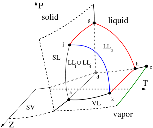
Figure 8: Schematic phase diagram for a value of $j_{s}$, for which only a tricritical line occurs. In this case, first-order phase transitions between liquid phases occur only between the superfluid and the normal fluid so that the model exhibits only a (blue) line of tricritical points (j-k). SL, VL, and SV are the surfaces of first-order phase transitions as described in Fig. 4. The superfluid dome is characterized by the vertices ’a’, ’k’, ’h’, ’g’, ’d’, and ’j’. Outside this region the liquid is a normal fluid. The surface LL₂ from Fig. 7 does not exist anymore and the transitions between liquid phases are either second-order phase transitions between the normal fluid and the superfluid mixed liquid (LL₃), or first-order phase transitions between the normal fluid and the superfluid liquid (LL${}_{1}\cup$LL₄). The surfaces LL₃ and LL${}_{1}\cup$LL₄ meet at the line j-k of tricritical points (blue line). The points ’g’ and ’h’ are critical end points, whereas ’j’ and ’k’ are tricritical end points. The point ’a’ is a quadruple point and ’d’ is a triple point.

If the coupling constant $j_{s}$ is increased further (Fig. 8), first-order phase transitions between liquid phases occur only between the superfluid and the normal fluid phase. There are no longer first-order demixing transitions between two normal fluids. Thus, upon increasing $j_{s}$, the surface LL${}_{3}\cup$LL₄ moves up (i.e., towards higher $P$ and $T$) so that accordingly the line i-f also moves up towards the line b-c. This implies that LL₂ shrinks and the wedge between the lines i-b and i-j becomes shorter. Finally LL₂ and b-c disappear and LL₁ and LL₄ become a single surface of first-order transitions between 4-rich superfluid and 3-rich normal liquid; this implies that the line i-f disappears, too. Accordingly, the phase diagram is left with only a (blue) line of tricritical points k-j. This topology of the phase diagram is shown in Fig. 8. In this case the liquid-liquid phase transitions are either second-order phase transitions on LL₃ between the normal fluid and the superfluid mixed liquid, or first-order phase transitions on LL${}_{4}\cup$LL₁ between the normal fluid and the superfluid liquid.

As discussed in the introduction, in the case of actual ${{}^{3}\text{He}}$ - ${{}^{4}\text{He}}$ mixtures the solid phase is formed only at high pressures, whereas for sufficiently low pressures the superfluid reaches down to $T=0.$ In order to obtain this topology from that of Fig. 8, by fiat one has to pull up and tilt the surface SL and to shift the superfluid dome down to $T=0$ so that the surface SV disappears. This transforms the phase diagram in Fig. 8 to the one shown in Fig. 3 such that g = ce⁺, h = ce, e = c, LL₃ = A₃, j-k = TC, j = tce⁺, k = tce, and LL${}_{1}\cup$LL₄ = A₄. In this sense the bulk phase diagram shown in Fig. 8 is supposed to mimic the one of the actual ${{}^{3}\text{He}}$- ${{}^{4}\text{He}}$ mixtures.

The demixing transitions at coexistence with the vapor phase for various sets of the coupling constants are shown in Figs. 9-12. In these figures the values of $c/k$ and $j/k$ are the same; only the value of $j_{s}$ is changed. For the choice of coupling constants $(c/k,j/k,j_{s}/k)=(1,5.714,1.717)$ (see Fig. 9), the phase diagram exhibits the topology of the schematic phase diagram shown in Fig. 6. The red line in Fig. 9(a) provides the temperature dependence of $X_{3}$ along the red line in Fig. 6 emanating from ’f’ towards ’h’. The green point ’e’ in Fig. 9 corresponds to the point ’f’ in Fig. 6 and the black point in Fig. 9 corresponds to the point ’c’ in Fig. 6. Because in Fig. 6 the red line h-f is a line of continuous phase transitions right up to the point ’f’, the line a-f-c does not exhibit a break in slope at ’f’. Below e, the liquid transitions are first-order transitions between the normal fluid and the superfluid liquid, whereas above e the demixing curve remains the same as in the case of $j_{s}=0$ (see Fig. 4).

Figure 9: Phase diagram for the coupling constants $(c/k,j/k,j_{s}/k)=(1,5.714,1.717)$ and $H=0$ corresponding to Fig. 6. Along the triple line a-f in Fig. 6 the figures show the coexistence between vapor, normal fluid, and superfluid (a) in the $(X^{l}_{3}$, $T)$ plane, with $X^{l}_{3}=\langle N_{3}\rangle/\mathcal{N}$ corresponding to the number density of 3-particles in the liquid phase, (b) in the $(X_{v}$, $T)$ plane at coexistence with the two liquid phases, where $X_{v}=(\langle N_{4}\rangle_{v}-\langle N_{3}\rangle_{v})/\mathcal{N}=\langle X_{4}^{v}\rangle-\langle X_{3}^{v}\rangle$ in the vapor phase, (c) in the $(D_{l}$, $T)$ plane, where $D_{l}=(\langle N_{4}\rangle_{l}+\langle N_{3}\rangle_{l})/\mathcal{N}$ is the total number density in the liquid phase, and (d) in the $(D_{v}$, $T)$ plane, where $D_{v}=(\langle N_{4}\rangle_{v}+\langle N_{3}\rangle_{v})/\mathcal{N}$ is the total number density in the vapor phase. The indices ’$l$’ and ’$v$’ refer to the values of the order parameters in the liquid and the vapor phase, respectively. Panels (e) and (f) show the temperature dependence of $P$ and $Z$ along the triple line a-c Fig. 6 (black) and along the red line f-h near ’f’ in Fig. 6. The red line is the line of second-order transitions between the normal fluid and superfluid at coexistence with vapor, which ends at the demixing curve at the green critical end point ’e’ (i. e., ’f’ in Fig. 6). At ’e’ the liquid state $(X^{\text{e}}_{l},D^{\text{e}}_{l},M^{\text{e}}_{l})=(0.773,0.994,0)$ coexists with the vapor state $(X^{\text{e}}_{v},D^{\text{e}}_{v},M^{\text{e}}_{v})=(-0.051,0.059,0)$ at $T_{\text{e}}/k=0.758$. N and S denote normal fluid and superfluid, respectively. The transitions between the vapor and the liquid phases are always first order. The points ’ce’ and ’e’ here correspond to the points ’c’ and ’f’ in Fig. 6.

As discussed in Fig. 7, for even larger values of $j_{s}$, both continuous and first-order superfluid transitions occur, giving rise to the occurrence of a line of tricritical points. For the choice of coupling constants $(c/k,j/k,j_{s}/k)=(1,5.714,2.231)$ and $(c/k,j/k,j_{s}/k)=(1,5.714,2.747)$ Figs. 10 and 11, respectively, show the liquid-liquid transitions at coexistence with the vapor phase for such a topology of the phase diagram. In both figures one finds two types of first-order liquid-liquid transitions. One between two normal liquids, which occur between ce and qp, and another one between the normal liquid phase and the superfluid liquid phase, which occur below tce. The points ’ce’, ’tce’, and ’qp’ in Figs. 10 and 11 correspond to the points ’c’, ’k’, and ’f’, respectively, in Fig. 7. The transitions between the two normal liquids correspond to the line f-c in Fig. 7, the transitions between the normal liquid and the superfluid correspond to the line a-f in Fig. 7, the small two phase region between ’tce’ and ’qp’ corresponds to the line f-k in Fig. 7, and the red line above ’tce’ corresponds to the red line emanating from ’k’ towards ’h’ in Fig. 7. In Fig. 7 the triple lines a-f and k-f merge at the quadrupole point ’qp’ = ’f’, where four phases coexist: two normal liquids, the superfluid, and the vapor phase. Below ’qp’, the liquid-liquid transitions at coexistence with the vapor phase are first-order transitions between the normal fluid and the superfluid. Upon increasing $j_{s}$ the tricritical end point tce = k is pulled towards higher temperatures (compare Figs. 10 and 11).

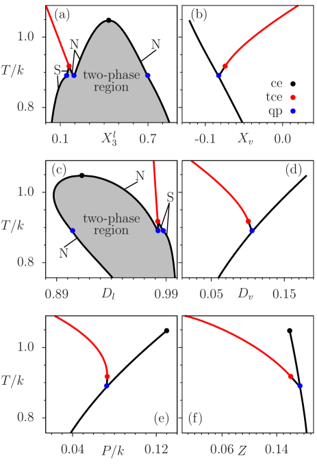
Figure 10: Phase diagram for the coupling constants $(c/k,j/k,j_{s}/k)=(1,5.714,2.231)$ and $H=0$ which corresponds to Fig. 7. Along the triple lines a-f and f-c in Fig. 7 the figures show the first-order demixing transitions of the liquid phase at coexistence with the vapor phase (a) in the $(X^{l}_{3}$, $T)$ plane, with $X^{l}_{3}=\langle N_{3}\rangle_{l}/\mathcal{N}$ as the number density of 3-particles in the liquid phase, (b) in the $(X_{v}$, $T)$ plane at coexistence of the vapor with the two liquid phases, where $X_{v}=(\langle N_{4}\rangle_{v}-\langle N_{3}\rangle_{v})/\mathcal{N}$ in the vapor phase, (c) in the $(D_{l}$, $T)$ plane, where $D_{l}=(\langle N_{4}\rangle_{l}+\langle N_{3}\rangle_{l})/\mathcal{N}$ in the liquid phase, and (d) in the $(D_{v}$, $T)$ plane, where $D_{v}=(\langle N_{4}\rangle_{v}+\langle N_{3}\rangle_{v})/\mathcal{N}$ in the vapor phase. The indices ’$l$’ and ’$v$’ refer to the values of the order parameters in the liquid and the vapor phase, respectively. Panels (e) and (f) show the temperature dependence of $P$ and $Z$ along the triple lines a-f, f-c, and f-k, in Fig. 7. The red line corresponds to second-order phase transitions between normal fluids and superfluids (line k-h in Fig. 7). At tce, the liquid state $(X^{\text{tce}}_{l},D^{\text{tce}}_{l},M^{\text{tce}}_{l})=(0.662,0.982,0)$ coexists with the vapor state $(X^{\text{tce}}_{v},D^{\text{tce}}_{v},M^{\text{tce}}_{v})=(-0.074,0.100,0)$ at $T_{\text{tce}}/k=0.917$. The point ce remains as in the case $j_{s}=0$. N and S denote normal liquid and superfluid, respectively. At the quadruple point ’qp’ the four coexisting states at $T_{\text{qp}}/k=0.887$ are two normal liquids $(X^{\text{qp}}_{l},D^{\text{qp}}_{l},M^{\text{qp}}_{l})=\{(-0.493,0.904,0),(0.594,0.982,0)\}$, a superfluid $(X^{\text{qp}}_{l},D^{\text{qp}}_{l},M^{\text{qp}}_{l})=(0.701,0.987,0.281)$, and the vapor state $(X^{\text{qp}}_{v},D^{\text{qp}}_{v},M^{\text{qp}}_{v})=(-0.082,0.105,0)$. The points ’ce’, ’tce’, and ’qp’ here correspond to the points ’c’, ’k’, and ’f’, respectively in Fig. 7. In (b), (d), (e), and (f), the long black coexistence curves are expected to exhibit a break in slope at ’qp’; on the present scales this is not visible.

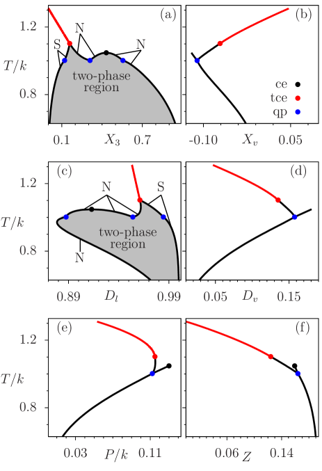
Figure 11: The same as in Fig. 10 but for the coupling constants $(c/k,j/k,j_{s}/k)=(1,5.714,2.747)$ and $H=0$. At tce the order parameters of the liquid and the vapor phases are $(X^{\text{tce}}_{l},D^{\text{tce}}_{l},M^{\text{tce}}_{l})=(0.644,0.961,0)$ and $(X^{\text{tce}}_{v},D^{\text{tce}}_{v},M^{\text{tce}}_{v})=(-0.071,0.135,0)$, respectively, and $T_{\text{tce}}/k=1.101$. Again, ce remains as in the case of $j_{s}=0$. N and S denote normal liquid and superfluid, respectively. The four coexisting states at the quadruple point ’qp’ are given by $(X^{\text{qp}},D^{\text{qp}},M^{\text{qp}})=(-0.222,0.888,0),(0.334,0.954,0),(0.742,0.984,0.456),\text{and }(0.110,0.157,0)$ at the temperature $T_{\text{qp}}/k=1.001$. The long black lines in (b) and (d) and the ones in (e) and (f) ending at ’ce’ are expected to exhibit a break in slope at ’qp’; on the present scales this is not visible.

In order to obtain phase diagrams with the topology illustrated in Fig. 8, one has to choose the coupling constants such that the demixing transitions at coexistence with the vapor phase occur only between the normal fluid and the superfluid. This means that in Fig. 7 the line f-c has to shrink to zero which implies that the critical point ’c’ coincides with the quadruple point ’f’. Within Fig. 11(a) this means that tce (= k in Fig. 7) has to be pulled up to higher temperatures such that the demixing critical end point ce (= c in Fig. 7) slides below the quadruple qp (= f in Fig. 7) so that the demixing phase transition between two normal fluids becomes an unstable one within the two-phase region of the superfluid and the mixed normal fluid (see Fig. 12(a)). For the coupling constants $(c/k,j/k)=(1,5.714)$ this is fulfilled, provided that $j_{s}/k>2.96$. For the coupling constants $(c/k,j/k,j_{s}/k)=(1,5.714,2.96)$ at $T_{\text{ce}}/k=1.047$ only three thermodynamic states coexist: the critical state $(X_{\text{ce}},D_{\text{ce}},M_{\text{ce}})=(0.050,0.913,0)$, the vapor phase, and a superfluid state $(X_{\text{s}},D_{\text{s}},M_{\text{s}})=(0.756,0.983,0.497)$. Accordingly, for coupling constants $(c/k=1,j/k=5.714,j_{s}/k>2.96)$ one obtains the type of phase diagram shown in Figs. 8 and 12.

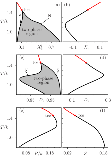
Figure 12: Phase diagrams for the coupling constants $(c/k,j/k,j_{s}/k)=(1,5.714,3.674)$ and $H=0$, corresponding to Fig. 8. The panels show the same as in Figs. 10 and 11; however the critical end point ’ce’ has disappeared. At tce the liquid state $(X^{\text{tce}}_{l},D^{\text{tce}}_{l},M^{\text{tce}}_{l})=(0.693,0.900,0)$ coexists with the vapor state $(X^{\text{tce}}_{v},D^{\text{tce}}_{v},M^{\text{tce}}_{v})=(0.010,0.176,0)$ at $T_{\text{tce}}/k=1.462$. For $T>T_{\text{tce}}$ there is only a second-order phase transition from a normal mixed liquid to a superfluid. For $T<T_{\text{tce}}$ the phase transitions between the normal fluid and the superfluid are first order. N and S denote normal liquids and superfluids, respectively.

As can be inferred from Fig. 12(f), upon increasing the temperature, the line of second-order phase transitions to the superfluid phase (red line) approaches the plane $Z=0$, where the liquid becomes pure ${{}^{4}\text{He}}$. In order to explore the phase diagram in the plane $Z=0$, in Eqs. (17) to (21) we have to take the limit $\mu_{3}\rightarrow-\infty$. In this limit $\Delta_{-}\rightarrow+\infty$ and $\Delta_{+}\rightarrow-\infty$ so that $W$ and $R$ turn into

$$\lim_{\mu_{3}\rightarrow-\infty}W(\Delta_{-},\Delta_{+},H,T)=0,\quad$$ (42)

and due to $\Delta_{-}+\Delta_{+}=\mu_{4}$

$$\lim_{\mu_{3}\rightarrow-\infty}R(\Delta_{-},\Delta_{+},H,T)=e^{\beta((c+k)X+(j+c)D+\mu_{4})}.\quad$$ (43)

Since $W_{\mu_{3}\rightarrow-\infty}=0$, due to Eqs. (17) and (18) one has $X_{\mu_{3}\rightarrow-\infty}=D_{\mu_{3}\rightarrow-\infty}$, where $D_{\mu_{3}\rightarrow-\infty}$ is given by

$$\begin{split}D_{\mu_{3}\rightarrow-\infty}&=\lim_{\mu_{3}\rightarrow-\infty}\frac{R(\Delta_{-},\Delta_{+},H,T)I_{0}(j_{s}M/T+H/T)}{1+R(\Delta_{-},\Delta_{+},H,T)I_{0}(j_{s}M/T+H/T)}\\ &=\frac{e^{\beta((j+k+2c)D+\mu_{4})}I_{0}(j_{s}M/T+H/T)}{1+e^{\beta((j+k+2c)D+\mu_{4})}I_{0}(j_{s}M/T+H/T)},\quad\end{split}$$ (44)

where, due to $X_{\mu_{3}\rightarrow-\infty}=D_{\mu_{3}\rightarrow-\infty}$, in $R_{\mu_{3}\rightarrow-\infty}$ we have replaced $X$ by $D$.

In this limit Eq. (29) reduces to

$$\frac{D}{M}=\frac{I_{0}(j_{s}M/T+H/T)}{I_{1}(j_{s}M/T+H/T)}$$ (45)

and the equilibrium free energy (Eq. (22)) reduces to

$$\phi(\mu_{3}\rightarrow-\infty,\mu_{4},H,T)=\frac{k+j+2c}{2}D^{2}+\frac{j_{s}}{2}M^{2}+T\ln(1-D).$$ (46)

In this limit the temperature of the superfluid transition is given by

$$T_{\text{s}}=\frac{j_{s}}{2}D,$$ (47)

and $\mu_{4}$ follows from Eq. (44):

$$\mu_{4}(H,T)=T\ln\frac{D}{1-D}-(j+2c+k)D-T\ln I_{0}(j_{s}M/T+H/T).$$ (48)

For pure ${{}^{4}\text{He}}$, i. e., for $Z=0$ and for the choice of the coupling constants $(c/k,j/k,j_{s}/k)=(1,5.714,3.674)$, the phase diagram in the $(T$, $P)$ plane is shown in Fig. 13. The dashed green line shows the $\lambda$-line of second-order phase transitions between normal liquids and superfluids. This line is terminated by the line of first-order liquid-vapor phase transitions (blue line) at the critical end point ce. The line of first-order liquid-vapor phase transitions ends at the critical point c. For high pressures the system becomes solid, (see Fig. 1) which, however, is not captured by the present model. Along the line of first-order liquid-vapor transitions ($T>T_{\text{ce}}$, blue line in Fig. 13), the difference between the number densities of the liquid and the vapor phase decreases upon increasing the temperature and vanishes at $T=T_{\text{c}}$. Accordingly, the two phases merge into a single phase at the critical point ’c’ given by

$$\frac{\text{d}\mu_{4}}{\text{d}D}|_{T}=\frac{\text{d}^{2}\mu_{4}}{\text{d}D^{2}}|_{T}=0\text{, }\quad\frac{\text{d}^{3}\mu_{4}}{\text{d}D^{3}}|_{T}>0\text{,}$$ (49)

where $\mu_{4}$ is given by Eq. (48). These conditions reduce to (note that $I_{0}(0)=1$)

$$D_{\text{c}}=0.5\text{,}\quad T_{\text{c}}=0.25(2c+j+k)\text{.}$$ (50)

For nonzero values of $Z$, i.e., in the presence of ${{}^{3}\text{He}}$ atoms, the critical points of the phase transitions between vapor and normal liquids ($M=0$) are given by (see Eqs. (5) and (27))

$$\frac{\mathrm{d}\Delta_{+}}{\mathrm{d}D}|_{\Delta_{-},T}=\frac{\mathrm{d}^{2}\Delta_{+}}{\mathrm{d}D^{2}}|_{\Delta_{-},T}=0\text{,}\quad\frac{\mathrm{d}^{3}\Delta_{+}}{\mathrm{d}D^{3}}|_{\Delta_{-},T}>0\text{,}$$ (51)

where in Eq. (27) also the partial derivatives of $X$ with respect to $D$ must be taken into account.

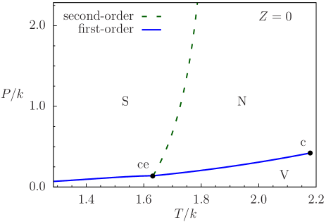
Figure 13: The $(T,P)$ phase diagram for the coupling constants $(c/k,j/k,j_{s}/k)=(1,5.714,3.674)$ and $H=0$ for pure ${{}^{4}\text{He}}$, i. e., $Z=0$. The dashed green line shows the $\lambda$-line of second-order phase transitions between normal liquids and superfluids. N, S, and V denote the normal liquid, the superfluid, and the vapor phase, respectively. The blue line of first-order liquid-vapor transitions terminates the $\lambda$-line at the critical end point ’ce’ and ends at the critical point ’c’ of the liquid-vapor coexistence line. ( We have been unable to find a set of coupling constants for which the dashed $\lambda$-line of second-order phase transitions exhibits a negative slope as it is the case for actual ${{}^{4}\text{He}}$.)

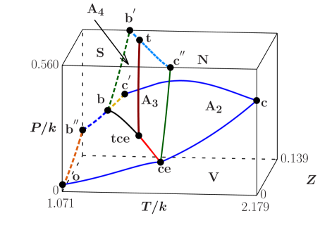
Figure 14: Numerical results for the fluid parts of the phase diagram for the choice of the coupling constants $(c/k,j/k,j_{s}/k)=(1,5.714,3.674)$ and $H=0$ in $(P$, $Z$, $T)$ space. The points o, ce, c, and c${}^{{}^{\prime\prime}}$ lie in the zero fugacity plane ($Z=0$) and the points c${}^{{}^{\prime\prime}}$, t, and b${}^{{}^{\prime}}$ lie in the constant pressure plane $P/k=0.560$. The points o and b${}^{{}^{\prime\prime}}$ have the same temperature $T/k=1.071$, while b, b${}^{{}^{\prime}}$, and c${}^{{}^{\prime}}$ share the same value of the fugacity $Z=0.139$. The surface (o-ce-tce-b-b${}^{{}^{\prime\prime}}$-o) corresponds to first-order phase transitions between the vapor phase (V) and the superfluid phase (S), whereas (ce-c-c${}^{{}^{\prime}}$-b-tce-ce) is the surface of first-order phase transitions between the vapor phase and the normal liquid phase (N); their union corresponds to A₂ in Fig. 3. The surface (b-tce-t-b${}^{{}^{\prime}}$-b) is the surface of first-order phase transitions between the superfluid and the normal liquid phase corresponding to A₄ in Fig. 3 and (tce-ce-c${}^{{}^{\prime\prime}}$-t-tce) is the surface of second-order phase transitions between the superfluid and the normal liquid phase corresponding to A₃ in Fig. 3. The black line b-tce and the light red line tce-ce are the lines of first- and second-order liquid-liquid transitions at coexistence with the vapor phase, respectively, which meet at the tricritical end point tce. The solid blue line c-c${}^{{}^{\prime}}$ is the line of critical points of the liquid-vapor phase transitions and the dark red curve (tce-t) is the line of tricritical points. The lowest pressure is $p/k=0$ whereas the highest temperature is $T/k=2.179$. The line o-b${}^{{}^{\prime\prime}}$ is the intersection of A₂ and the plane $T/k=1.071$, the line c${}^{{}^{\prime}}$-b-b${}^{{}^{\prime\prime}}$ is the intersection of A₂ and the plane $Z=0.139$; the line b-b${}^{{}^{\prime}}$ is the intersection of A₄ with the plane $Z=0.139$; the line b${}^{{}^{\prime}}$-t and t-c${}^{{}^{\prime\prime}}$ are the intersection of A₄ and A₃, respectively, with the plane $P/k=0.560$. We note that at ’ce’ the line o-ce-c does not exhibit a break in slope (see Fig. 13).

Having determined various features of the phase diagram of the present model for a set of coupling constants for which the topology of the phase diagram is that of the experimental one, we can illustrate quantitatively the phase diagram in the $(P$, $Z$, $T)$ space. The phase diagram, which – for a suitable set of coupling constants – resembles the schematic phase diagram proposed in Ref. Krech and Dietrich (1992a) and exhibits all relevant fluid phases, is given in Fig. 14 (compare Fig. 3). Accordingly, Fig. 14 shows where the vapor phase (V), the normal liquid phase (N), and the superfluid phase are thermodynamically stable and where first- or second-order phase transitions among each other occur. The transitions between the vapor and the liquid phases are given by the two surfaces o-ce-tce-b-b${}^{{}^{\prime\prime}}$-o and ce-c-c${}^{{}^{\prime}}$-b-tce-ce (the union of which corresponds to $\text{A}_{2}$ in Fig. 3), while the loci of the phase transitions between the superfluid and the normal fluid form the two surfaces b-tce-t-b${}^{{}^{\prime}}$-b and tce-ce-c${}^{{}^{\prime\prime}}$-t-tce which in Fig. 3, correspond to $\text{A}_{4}$ and $\text{A}_{3}$, respectively.

The points o, ce, c, and c${}^{{}^{\prime\prime}}$ lie in the zero fugacity plane ($Z=0$) whereas b${}^{{}^{\prime}}$, t, and c${}^{{}^{\prime\prime}}$ lie in the plane of constant pressure $P/k=0.560$. The points b${}^{{}^{\prime\prime}}$ and o are located in the plane of constant temperature $T/k=1.071$, while b, b${}^{{}^{\prime}}$, b${}^{{}^{\prime\prime}}$, and c${}^{{}^{\prime}}$ share the same value of fugacity $Z=0.139$. The black line b-tce and the light red line tce-ce indicate first- and second-order liquid-liquid phase transitions, respectively, at coexistence with the vapor phase. These two lines are connected at the tricritical end point tce. The dark red solid line (tce-t) connects the surfaces A₄ and A₃ of first- and second-order liquid-liquid phase transitions ((b-b${}^{{}^{\prime}}$-t-tce-b) and (t-tce-ce-c${}^{{}^{\prime\prime}}$-t)), respectively. The coexisting states along the two lines (b-tce, $T<T_{\text{tce}}$) and (tce-ce, $T>T_{\text{tce}}$) are the ones shown in Fig. 12. The solid blue line (c-c${}^{{}^{\prime}}$) is the line of critical points of the liquid-vapor phase transitions and the dark red curve (tce-t) is the line of tricritical points with the tricritical end point tce.

By moving along the line b-b${}^{{}^{\prime\prime}}$ towards b${}^{{}^{\prime\prime}}$ the number density in the liquid phase increases. This implies that the larger the number density of the liquid phase at b is, the shorter is the line b-b${}^{{}^{\prime\prime}}$ (note that $D<1$). This means that, by lowering the temperature along the line of first-order liquid-liquid phase transitions at coexistence with the vapor phase (tce-b), the point b shifts towards the point b${}^{{}^{\prime\prime}}$.

The liquid-liquid phase transitions at constant pressure are given by the curve b${}^{{}^{\prime}}$-t-c${}^{{}^{\prime\prime}}$. The curve (b${}^{{}^{\prime}}$-t) is a line of first-order liquid-liquid phase transitions at constant pressure, which is connected to the line of second-order liquid transitions (t-c${}^{{}^{\prime\prime}}$) at the tricritical point t. The coexisting states along these two lines are shown in Fig. 15. For even higher pressures the system solidifies, and the two surfaces (A₄, b-tce-t-b${}^{{}^{\prime}}$-b) and (A₃, tce-ce-c${}^{{}^{\prime\prime}}$-t-tce) should continue towards a surface of first-order liquid-solid phase transitions (see A₁ in Fig. 3) which is not supported by the present model.

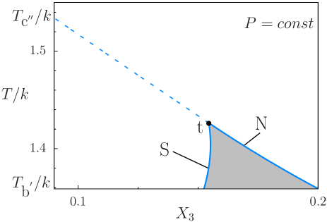
Figure 15: The liquid-liquid phase transitions at fixed pressure $P/k=0.560$ in the $(X_{3}$, $T)$ plane for the choice of the coupling constants $(c/k,j/k,j_{s}/k)=(1,5.714,3.674)$ and $H=0$. The figure provides the temperature dependence of $X_{3}$ along the line b${}^{{}^{\prime}}$-t-c${}^{{}^{\prime\prime}}$ in Fig. 14. For $T_{\text{t}}<T<T_{\text{c${}^{{}^{\prime\prime}}$}}$ the light blue dashed line represents continuous phase transitions whereas for $T_{\text{b${}^{{}^{\prime}}$}}<T<T_{\text{t}}$ the lines indicate the coexisting superfluid (S) and normal liquid (N) states at first-order phase transitions. The two-phase region is shaded in grey. The point t corresponds to a tricritical point.

V Summary and Conclusion

The phase diagram of the general vectorized Blume-Emery-Griffiths model has been explored within mean-field theory. The model exhibits a liquid phase, which can be either a superfluid or a normal liquid, and a vapor phase. Depending on the choice of the coupling constants the model exhibits various topologies of the phase diagram. Here we have focused on those topologies of the phase diagram which are associated with liquid-liquid phase transitions at coexistence with the vapor phase. Knowledge of them is a prerequisite for studying tricritical Casimir forces in ${{}^{3}\text{He}}$ -${{}^{4}\text{He}}$ wetting films. If the coupling constant $j_{s}$, which facilitates the occurrence of the superfluid phase, is turned off, the phase diagram is that of a normal binary liquid mixture (see Figs. 4 and 5). For nonzero but small values of this superfluid coupling constant the transitions to the superfluid phase are second order only (Figs. 6 and 9). For larger values of this coupling constant, the transition to the superfluid phase can also be of first order (Figs. 7, 10, and 11); the liquid-liquid phase transitions can be either between two normal liquids or between superfluid and normal liquids. For even larger values of the superfluid coupling constant, the first-order liquid-liquid phase transitions occur only between the superfluid and the normal fluid (Figs. 8 and 12), as it is the case for actual ${{}^{3}\text{He}}$ -${{}^{4}\text{He}}$ mixtures (see Figs. 1-3).

We conclude that for a suitable set of coupling constants, various features of the phase diagram of ${{}^{3}\text{He}}$ -${{}^{4}\text{He}}$ mixtures are captured by the present approach (see Figs. 12-15). The detailed knowledge of the bulk phase diagram is necessary for studying wetting phenomena within the present model and, further, tricritical Casimir forces acting on wetting films. The present model lends itself also for investigations based on Monte Carlo simulations. This model of a binary liquid mixture incorporates vectorial degrees of freedom associated with the ${{}^{4}\text{He}}$ particles which covers the more complex behavior of the superfluid order parameter. It is interesting to note that the sequence of the phase diagrams (Fig. 9(a), 10(a), 11(a), 12(a)) exhibits the identical topologies as the phase diagrams of one-component dipolar fluids upon increasing the dipole strength with the isotropic and ferromagnetic liquid corresponding to the normal liquid and the superfluid, respectively Groh and Dietrich (1994a, b). For dipolar fluids the solid phase can be captured by off-lattice density functional theory Groh and Dietrich (1996).

References

- Krech and Dietrich (1992a) M. Krech and S. Dietrich, Phys. Rev. A 46, 1922 (1992a).
- Blume et al. (1971) M. Blume, V. J. Emery, and R. B. Griffiths, Phys. Rev. A 4, 1071 (1971).
- Sivardière and Lajzerowicz (1975) J. Sivardière and J. Lajzerowicz, Phys. Rev. A 11, 2090 (1975).
- Dietrich and Latz (1989) S. Dietrich and A. Latz, Phys. Rev. B 40, 9204 (1989).
- Getta and Dietrich (1993) T. Getta and S. Dietrich, Phys. Rev. E 47, 1856 (1993).
- Mukamel and Blume (1974) D. Mukamel and M. Blume, Phys. Rev. A 10, 610 (1974).
- Cardy and Scalapino (1979) J. L. Cardy and D. J. Scalapino, Phys. Rev. B 19, 1428 (1979).
- Berker and Nelson (1979) A. N. Berker and D. R. Nelson, Phys. Rev. B 19, 2488 (1979).
- Maciołek et al. (2004) A. Maciołek, M. Krech, and S. Dietrich, Phys. Rev. E 69, 036117 (2004).
- Garcia and Chan (2002) R. Garcia and M. H. W. Chan, Phys. Rev. Lett. 88, 086101 (2002).
- Krech and Dietrich (1992b) M. Krech and S. Dietrich, Phys. Rev. A 46, 1886 (1992b).
- Garcia and Chan (1999) R. Garcia and M. H. W. Chan, Phys. Rev. Lett. 83, 1187 (1999).
- Ganshin et al. (2006) A. Ganshin, S. Scheidemantel, R. Garcia, and M. H. W. Chan, Phys. Rev. Lett. 97, 075301 (2006).
- Maciołek et al. (2007) A. Maciołek, A. Gambassi, and S. Dietrich, Phys. Rev. E 76, 031124 (2007).
- Chaikin and Lubensky (1995) P. M. Chaikin and T. Lubensky, Principles of condensed matter physics (Cambridge University press, Cambridge, 1995).
- Abramowitz and Stegun (1972) M. Abramowitz and I. A. Stegun, eds., Handbook of mathematical functions (Dover, New York, 1972).
- Groh and Dietrich (1994a) B. Groh and S. Dietrich, Phys. Rev. Lett. 72, 2422 (1994a).
- Groh and Dietrich (1994b) B. Groh and S. Dietrich, Phys. Rev. E 50, 3814 (1994b).
- Groh and Dietrich (1996) B. Groh and S. Dietrich, Phys. Rev. E 54, 1687 (1996).