ON PERIODIC PERTURBATIONS OF ASYMMETRIC DUFFING–VAN-DER-POL EQUATION

Abstract

Time-periodic perturbations of an asymmetric Duffing–Van-der-Pol equation close to an integrable equation with a homoclinic “figure-eight” of a saddle are considered. The behavior of solutions outside the neighborhood of “figure-eight” is studied analytically. The problem of limit cycles for an autonomous equation is solved and resonance zones for a nonautonomous equation are analyzed. The behavior of the separatrices of a fixed saddle point of the Poincaré map in the small neighborhood of the unperturbed “figure-eight” is ascertained. The results obtained are illustrated by numerical computations.

1 Introduction

The theory of time-periodic systems close to two-dimensional nonlinear Hamiltonian systems has been greatly advanced by now (see, e.g., Guckenheimer & Holmes, [1983], Morozov & Shil’nikov, [1983], Wiggins, [1990], Morozov, [1998]). However, many problems remain unsolved, and new examples should be addressed. In this paper, we will consider one such example – an asymmetric variant of the classical Duffing–Van-der-Pol equation:

$$\ddot{x}+\alpha x+\beta x^{3}=\varepsilon[(\gamma_{1}+\gamma_{2}x+\gamma_{3}x^{2})\dot{x}+\gamma_{4}\sin{\gamma_{5}t}],$$ (1)

where $\alpha,\beta,\gamma_{1}\div\gamma_{5}$ are parameters, and $\varepsilon$ is a small positive parameter. It is always possible to set $\alpha=\pm 1,\beta=\pm 1$ in Eq.  (1). Naturally, the case $\alpha=\beta=-1$ is of no interest to us. In the cases $\alpha=1,\beta=\pm 1$, the asymmetric perturbation term $\gamma_{2}x\dot{x}$ does not play a significant role, it is essential only in the case $\alpha=-1,\beta=1$. Equation (1) for $\alpha=1,\beta=\pm 1$ was studied in ample detail (see, e.g., Morozov, [1973], Morozov & Shil’nikov, [1975], Morozov, [1976], Morozov, [1993], Morozov, [1998]). Therefore, we will address the case $\alpha=-1,\beta=1$. The phase plane of an unperturbed equation has two saddle separatrix loops $O(0,0)$ forming “figure-eight” (Fig. 1). Of the three parameters $\gamma_{1},\gamma_{2},\gamma_{3}$ one may be excluded to yield the following equation

$$\ddot{x}-x+x^{3}=\varepsilon[(p_{1}+p_{2}x-x^{2})\dot{x}+p_{3}\sin{p_{4}t}],$$ (2)

where $p_{1}\div p_{4}$ are parameters. An analysis of Eq. (2) implies the solution of the following tasks: 1) for the autonomous equation ($p_{3}=0$) – partition the plane of the parameters $(p_{1},p_{2})$ into regions with different topological structures and specify the structures; 2) for the nonautonomous equation ($p_{3}\neq 0$) – determine possible structures of resonance zones outside the neighborhood of “figure-eight” and the conditions of existence of structurally stable and unstable homoclinic Poincaré structures in the neighborhood of “figure-eight”. The existence of a homoclinic structure specifies complicated behavior of solutions, in other words, it leads to chaos. Bifurcations in the neighborhood of “figure-eight” at a nonzero saddle value of the unperturbed autonomous system were recently considered in Gonchenko et al., [2013].

The Duffing–Van-der-Pol equation is widely used in the theory of oscillations (see, e.g., Morozov, [1973], Guckenheimer & Holmes, [1983], Morozov, [1998]). Along with numerous applied problems in which there arises Eq. (2), we can mention a purely mathematical problem of vector field bifurcations on a plane that are invariant to the turn of angle $\pi$ Arnold, [1978]. In this problem, in Eq. (1) we have $\gamma_{2}=\gamma_{4}=0$ and the coefficients of the linear terms $\alpha x+\varepsilon\gamma_{1}\dot{x}$, unlike our case, are the parameters of deformation. Note also the work Bautin, [1975] (as well as Bautin & Leontovich, [1976]) where an autonomous system with cubic nonlinearity without small parameter describing an electric circuit with tunnel diode was considered. Possible local bifurcations were determined and phase portraits were constructed to an accuracy of an even number of limit cycles.

The presence of the term $p_{2}x\dot{x}$ in Eq. (2) greatly complicates the problem: there may exist in the autonomous equation ($p_{3}=0$) two limit cycles enclosing any of the equilibrium states $O_{\pm}(\pm 1,0)$, or a “big” separatrix loop enclosing the equilibrium states $O_{\pm}(\pm 1,0)$ that is absent in the unperturbed equation Morozov & Fedorov, [1976], Kostromina & Morozov, [2012].

Fig. 1: Phase portrait of unperturbed equation.

Solution of problems 2) and 3) rests upon the solution of problem 1). Therefore, we will start with the first problem.

2 Investigation of an autonomous equation

2.1 Poincaré–Pontryagin generating functions

The first integral of the unperturbed equation is $H(x,y)\equiv y^{2}/2-x^{2}/2+x^{4}/4=h$. The values $h\in(-0.25,0)$ correspond to the domains $G^{\pm}_{1}$ inside “figure-eight”, and $h>0$ to the domain $G_{2}$ outside “figure-eight” (Fig.  1). The value $h=0$ corresponds to two symmetric saddle loops (“figure-eight”).

The main problem in studying Eq. (2) for $p_{3}=0$ is limit cycles. Its solution results in finding real zeros of the Poincaré–Pontryagin generating functions $B(h)$ Morozov, [1998].

According to Kostromina & Morozov, [2012], we have

$$\begin{split}B_{1}=B_{1}^{\pm}(\rho(h))&=\frac{4}{30\pi(2-\rho)^{5/2}}\{2(5p_{1}-1)(\rho-1)(2-\rho){\bf K}(k)+\\ &+\left[5p_{1}(2-\rho)^{2}-4(\rho^{2}-\rho+1)\right]{\bf E}(k)\pm\frac{15p_{2}\sqrt{2}}{16}\pi\rho^{2}\sqrt{2-\rho}\}\equiv\\ &\equiv\frac{4}{30\pi(2-\rho)^{5/2}}B_{10}^{\pm}(\rho)\end{split}$$ (3)

for the domains $G_{1}^{\pm}$ and

$$\begin{split}B_{2}&=B_{2}(\rho(h))=\frac{8}{30\pi(2\rho-1)^{5/2}}\left\{\left[5p_{1}(2\rho-1)(1-\rho)-2(\rho-1)(2-\rho)\right]\right.{\bf K}(k)+\\ &+\left.\left[5p_{1}(2\rho-1)^{2}-4(\rho^{2}-\rho+1)\right]{\bf E}(k)\right\}\equiv\frac{8}{30\pi(2\rho-1)^{5/2}}B_{20}(\rho)\end{split}$$ (4)

for the domain $G_{2}$. Here, ${\bf K}(k),{\bf E}(k)$ are complete elliptic integrals and $\rho=k^{2}$. Note that $\rho$ is a more convenient variable than $h$. In the formula (3) we have $\rho(h)=2\sqrt{1+4h}/(1+\sqrt{1+4h})$ ($\rho\in(0,1)$), and in (4) we have $\rho(h)=(1+\sqrt{1+4h})/2\sqrt{1+4h}$ ($\rho\in(1/2,1)$); $\rho=1$ corresponds to “figure-eight”. Note that the function $B_{2}(\rho)$ does not depend on the parameter $p_{2}$.

2.2 Limit cycles

Investigation of the functions $B_{1}^{\pm}(\rho),B_{2}(\rho)$ gives the following results Kostromina & Morozov, [2012].

Theorem 2.1.

For sufficiently small $\varepsilon$, the number of limit cycles in each domain $G_{1}^{\pm}$ and $G_{2}$ of Eq. (2) does not exceed two.

Theorem 2.2.

For sufficiently small $\varepsilon$, the number of limit cycles of Eq. (2) does not exceed three.

The authors of Kostromina & Morozov, [2012] partitioned the parameter plane into 22 domains $D_{m}$, $m=1,\ldots,22$, gave the basic phase portraits at different values of parameters from those domains and found all bifurcations.

By virtue of the invariance of Eq. (2) to the change $(p_{2},x,y)\to(-p_{2},-x,-y)$ the partitioning of the plane of the parameters $(p_{1},p_{2})$ is symmetric to the $p_{1}$ axis. Therefore, only the upper half plane $p_{2}\geq 0$ containing 13 domains $D_{m}$, $m=1,\ldots,13$ is shown in Fig. 2. A magnified fragment of Fig. 2 is presented schematically in Fig. 3. By virtue of the symmetry, the phase portraits for the domain $p_{2}<0$ are obtained by the turn of angle $\pi$ of the corresponding phase portrait from the domain $p_{2}>0$.

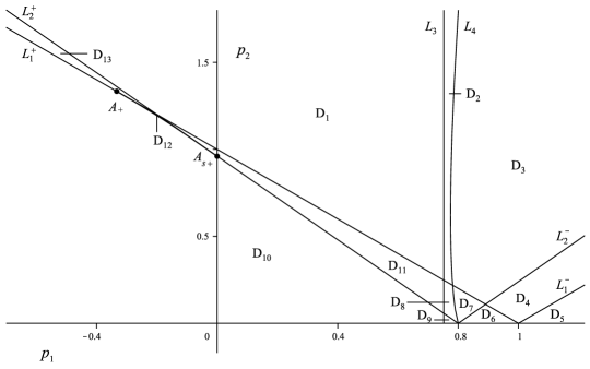
Fig. 2: Partition of the plane of parameters $(p_{1},p_{2})$ into domains with different phase portrait topology.

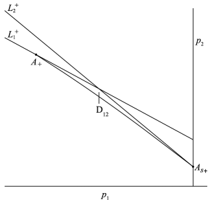
Fig. 3: Magnified fragment of Fig. 2.

Let us introduce the notation $(i,j,k)$ that means the existence of $i$ limit cycles inside the right loop, $j$ inside the left loop, and $k$ outside “figure-eight”. It was proved that $D_{1}$ is of the type $(0,0,0);D_{2}-(0,0,2),D_{3}-(0,0,1);D_{4}-(0,1,1);D_{5}-(0,0,1);D_{6}-(1,1,1);D_{7}-(1,0,1);D_{8}-(1,0,2);D_{9}-(0,0,2);D_{10}-(0,0,0);D_{11}-(1,0,0);D_{12}-(2,0,0);D_{13}-(1,0,0)$.

The notation of the bifurcation lines in Fig. 2:

$L_{1}^{\pm}:p_{1}\pm p_{2}-1=0$ – straight lines at which the autonomous equation has structurally unstable foci $O_{\pm}(\pm 1,0)$ in domains $G_{1}^{\pm}$, respectively.

$A_{+}(-\frac{1}{3},\frac{4}{3})$ – the point on the straight line $L_{1}^{+}$ from which the double cycle line originates. The double cycle line is plotted using the system $B_{10}^{+}(\rho,p_{1},p_{2})=0,[dB_{10}^{+}(\rho,p_{1},p_{2})/d\rho]=0$, $\rho\in(0,1)$; the point $A_{+}$ corresponds to $\rho=0$. This point is readily found by the power series expansion of the function $B_{10}^{+}(\rho)$ in the neighborhood of $\rho=0$ in the case of a structurally unstable focus and zero first Lyapunov exponent (with the second Lyapunov exponent being nonzero). The extreme point $A_{s+}(0,0.96)$ of the double cycle line corresponds to $\rho=1$ (see Fig. 3). When the saddle value $\sigma_{c}=\varepsilon p_{1}$ vanishes to zero at $p_{1}=0$ the double cycle merges with the separatrix.

$L_{2}^{\pm}:5p_{1}\pm\frac{15\sqrt{2}\pi}{16}p_{2}-4=0$ – straight lines on which the autonomous equation has separatrix loops (right, left) of saddle $O(0,0)$ in domains $G_{1}^{\pm}$. These straight lines are given by the Melnikov formula for autonomous systems.

$L_{3}$ – double cycle line in domain $G_{2}$ corresponding to the bifurcation value $p_{1}\approx 0.7523$.

$L_{4}$ – line of the “big” loop of the separatrix of saddle $O(0,0)$. This line was plotted numerically using the WInSet software Morozov & Dragunov, [2003].

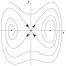
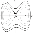
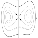
(a)	(b)	(c)
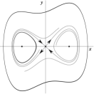
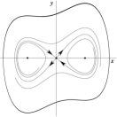
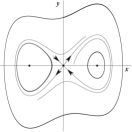
(d)	(e)	(f)
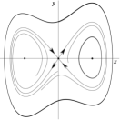
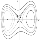
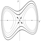
(g)	(h)	(i)
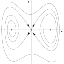
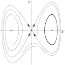
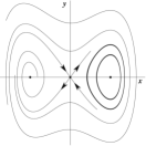
(j)	(k)	(l)
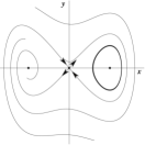
(m)

Fig. 4: Basic phase portraits of perturbed autonomous equation in domains $D_{1}$ (a); $D_{2}$ (b); $D_{3}$ (c); $D_{4}$ (d); $D_{5}$ (e); $D_{6}$ (f); $D_{7}$ (g); $D_{8}$ (h); $D_{9}$ (i); $D_{10}$ (j); $D_{11}$ (k); $D_{12}$ (l); $D_{13}$ (m).

Basic phase portraits of a perturbed autonomous equation for the parameter values from 13 domains on the $(p_{1},p_{2})$ plane are presented in Fig. 4. The dots show the equilibrium states ($(0,0)$ saddle point and $(\pm 1,0)$ focus), the arrows indicate directions of motion on the separatrices. Note also that the limit cycle near “figure-eight” is unstable. The other phase portraits for symmetric domains may be obtained by rotation of angle $\pi$. The simplest phase portraits are obtained for the dissipation domain $D_{10}$.

3 Analysis of resonance zones topology

In the domains filled with closed phase curves of the unperturbed equation ($\varepsilon=0$) and separated from the unperturbed separatrices, we will pass in Eq. (2) to the “$I$ action–$\theta$ angle ” variables by the following formulas

$$\begin{split}&I(h)={1\over 2\pi}\oint y(x,h)dx,\\ &\theta={\partial S(x,I)\over\partial I},S=\int_{x_{0}}^{x}y(x,h(I))dx,\end{split}$$ (5)

where $S(x,I)$ is the generating function of this canonical transformation. The resulting system will be written in the form

$$\begin{split}\dot{I}&=\varepsilon[(p_{1}+p_{2}x-x^{2})y+p_{3}\sin{\varphi}]x^{\prime}_{\theta}\equiv\varepsilon F_{1}(I,\theta,\varphi),\\ \dot{\theta}&=\omega(I)+\varepsilon[(p_{1}+p_{2}x-x^{2})y+p_{3}\sin{\varphi}]x^{\prime}_{I}\equiv\omega(I)+\varepsilon F_{2}(I,\theta,\varphi),\\ \dot{\varphi}&=p_{4},\end{split}$$ (6)

where $\omega$ is the frequency of self-excited oscillations. Consider the resonance case when

$$\omega(I_{pq})=(q/p)p_{4},$$ (7)

where $p,q$ are coprime integer numbers. The level $I=I_{pq}$ (closed phase curve $H(x,y)=h_{pq}$ of the unperturbed system) will be referred to as the resonance level. The neighborhood $U_{\sqrt{\varepsilon}}=\{(I,\theta):I_{pq}-C\sqrt{\varepsilon}<I<I_{pq}+C\sqrt{\varepsilon},\ 0\leq\theta<2\pi,\ C=const>0\}$ will be called the resonance zone.

By the substitution

$$\theta=\psi+(q/p)\varphi,\quad I=I_{pq}+\mu\eta,\quad\mu=\sqrt{\varepsilon},$$ (8)

in (6), by averaging the obtained system over the fast variable $\varphi$ and neglecting the terms $O(\mu^{3})$, we obtain the system Morozov, [1998]

$$\dot{u}=\mu A_{0}(v,I_{pq})+\mu^{2}P_{0}(v,I_{pq})u,$$ (9)

$$\dot{v}=\mu bu+\mu^{2}(b_{1}u^{2}+Q_{0}(v,I_{pq})),$$

where $u=\eta+O(\mu),v=\psi+O(\mu^{2})$, $b=d\omega(I_{pq})/dI,b_{1}=d^{2}\omega(I_{pq})/2dI^{2}$,

$$A_{0}(v,I_{pq})={1\over 2\pi p}\int^{2\pi p}_{0}F_{1}(I_{pq},v+q\varphi/p,\varphi)d\varphi,$$ (10)

$$P_{0}(v,I_{pq})={1\over 2\pi p}\int^{2\pi p}_{0}[\partial F_{1}(I_{pq},v+q\varphi/p,\varphi)/\partial I]d\varphi,$$ (11)

$$Q_{0}(v,I_{pq})={1\over 2\pi p}\int^{2\pi p}_{0}F_{2}(I_{pq},v+q\varphi/p,\varphi)d\varphi.$$ (12)

The substitution $u\to u-\mu Q_{0}(v,I_{pq})/b$ and the transition to “slow time” $\tau=\mu t$ reduces Eqs.  (9) to a pendulum equation Morozov, [1998]

$${d^{2}v\over d\tau{}^{2}}-bA_{0}(v,I_{pq})=\mu\sigma(v,I_{pq}){dv\over d\tau},$$ (13)

where

$$\sigma(v,I_{pq})={1\over 2\pi p}\int^{2\pi p}_{0}(p_{1}+p_{2}x-x^{2})_{\left|{\begin{array}[]{c}x=x(I_{pq},v+q\varphi/p)\\ y=y(I_{pq},v+q\varphi/p)\end{array}}\right.}d\varphi.$$ (14)

Apparently, $\sigma=const$.

The topology of individual resonance zones may be found from Eq. (13) to an accuracy of terms of order $\mu^{2}$.

In calculations of the function $A_{0}(v,I_{pq})$ and quantities $b$ and $\sigma$ we distinguish the following cases.

Case 1 : $(x,y)\in G_{1}^{\pm}=\{(x,y):y^{2}/2-x^{2}/2+x^{4}/4=h,h\in(-0.25,0)\}$;

Case 2 : $(x,y)\in G_{2}=\{(x,y):y^{2}/2-x^{2}/2+x^{4}/4=h,h>0\}$.

The unperturbed solution in (6) is different in each case Kostromina & Morozov, [2012].

We represent the function $A_{0}(v,I_{pq})$ in the form $A_{0j}(v,I_{pq})=\widetilde{A}_{0j}(v,I_{pq})+B_{j}(I_{pq})$ and designate $b=b_{j},\sigma=\sigma_{j},j=1,2$, where $B_{1},B_{2}$ are the Poincaré–Pontryagin generating functions (3) and (4), respectively.

Following Morozov, [1998], we refer to the resonance level $I=I_{pq}$ as splittable if the equation $A_{0j}(v;I_{pq})=0$ has simple roots. The nonsplittable resonance level $I=I_{pq}$ for which $|A_{0j}(v;I_{pq})|>0$ is called passable. The splittable resonance level $I=I_{pq}$ is called partially passable, if $B_{j}(I_{pq})\neq 0$ and impassable, if $B_{j}(I_{pq})=0$.

Note that the behavior of solutions of the initial equation (2) in the neighborhood of passable, partially passable and impassable resonance levels is defined by the theorems from Morozov, [1998].

3.1 Case 1

Using the unperturbed solutions at the resonance level and formulas (10), (14), we find for $q=1$

$${d^{2}v\over d\tau^{2}}-b_{1}(p_{3}A_{1}\cos{pv}+B_{1})=\mu\sigma_{1}{dv\over d\tau},$$ (15)

where

$$b_{1}=\frac{\pi}{2}\frac{(2-\rho)^{3/2}[2(1-\rho){\bf K}(\rho)-(2-\rho){\bf E}(\rho)]}{\rho^{2}(1-\rho){\bf K}^{2}(\rho)},$$ (16)

$$\sigma_{1}=p_{1}-\frac{2}{(2-\rho){\bf K}(\rho)}{\bf E}(\rho),$$ (17)

$$A_{1}=-\sqrt{2}p_{4}\frac{a^{p}}{1+a^{2p}},a=exp\left(-\pi\frac{{\bf K}(\sqrt{1-\rho})}{{\bf K}(\rho)}\right).$$ (18)

For $q>1$ we obtain the equation

$${d^{2}v\over d\tau^{2}}-b_{1}B_{1}=\mu\sigma_{1}{dv\over d\tau}.$$ (19)

Thus, for $q=1$ the topology of resonance zones is described by Eq. (15). The phase portraits of this equation are well known Morozov, [1998] (Fig. 5). At $B_{1}(I_{pq})=0$, we have by definition an impassable resonance (Fig. 5(c)). In this case, the resonance level $I=I_{pq}$ coincides with the level $I=I_{0}$ in the neighborhood of which the autonomous equation has a limit cycle. A partially passable resonance is presented in Fig. 5(b), and a passable resonance in Fig. 5(a). According to (19), at $q>1$ and $B_{1}(I_{pq})\neq 0$ we have a passable resonance.

Consider briefly the bifurcations of the transition from the impassable to the partially passable resonance. Let us set in Eq. (15) $B_{1}=\mu\gamma$, where $\gamma$ defines the deviation of the resonance level $I=I_{pq}$ from $I=I_{0}$. We denote by $\gamma^{\pm}$ the bifurcation values of $\gamma$ at which Eq. (15) has, respectively, the upper or lower loop enclosing a phase cylinder. As $\gamma$ deviates from the bifurcation value, the loop gives birth to a limit cycle enclosing a phase cylinder, and the resonance level becomes partially passable. The limit cycle corresponds to the two-dimensional torus in the initial equation (for the Poincaré map it is a closed invariant curve shown in Fig. 6). More details about these bifurcations can be found in Morozov, [1998].

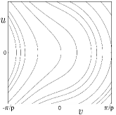
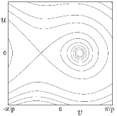
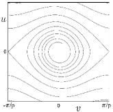
(a)	(b)	(c)

Fig. 5: Phase portraits for Eq. (15).

The frequency $\omega(I)$ of the self-excited oscillations in domains $G_{1}^{\pm}$ meets the condition $\omega(I)\in(0,\sqrt{2})$ and is a monotonic function. Then from the resonance condition (7) follows $p>p_{4}/\sqrt{2}$. Therefore, only the resonance levels $H(x,y)=y^{2}/2-x^{2}/2+x^{4}/4=h_{p1}$, for which $p>p_{4}/\sqrt{2}$, are split. Note that the resonance levels with larger values of $p$ are closer to the unperturbed separatrix.

3.2 Case 2

Analogously to Case 1, we find the equation

$${d^{2}v\over d\tau{}^{2}}-b_{2}(p_{3}A_{2}\cos{pv}+B_{2})=\mu\sigma_{2}{dv\over d\tau},$$ (20)

that defines the topology of the resonance zones at odd $p$ and $q=1$. Otherwise, the resonance zones topology is defined by the equation

$${d^{2}v\over d\tau{}^{2}}-b_{2}B_{2}=\mu\sigma_{2}{dv\over d\tau}.$$ (21)

In (20) and (21) we have

$$b_{2}=\frac{\pi}{4}\frac{(2\rho-1)^{3/2}[(1-\rho){\bf K}(\rho)+(2\rho-1){\bf E}(\rho)]}{\rho(1-\rho){\bf K}^{2}(\rho)},$$ (22)

$$\sigma_{2}=p_{1}-\frac{2}{(2\rho-1){\bf K}(\rho)}({\bf E}(\rho)+(\rho-1){\bf K}(\rho)),$$ (23)

$$A_{2}=-2\sqrt{2}p_{4}\frac{a^{p/2}}{1+a^{p}}.$$ (24)

For even $p$ and/or $q>1$, the resonance is passable if $B_{2}(I_{pq})\neq 0$.

The Poincaré map for Eq. (2) at different parameter values was constructed using the WInSet software Morozov & Dragunov, [2003]. It was found that at small values of $\varepsilon$ numerical results are in a good agreement with the theoretical study. Figure 6 illustrates the structure of the neighborhood of the splittable levels $I=I_{21},I=I_{31}$. The impassable resonance zones are shown in Figs. 6(a) and 6(c), and the partially passable zones in Figs. 6(b) and 6(d). The dots in Fig. 6 correspond to points of period-2, as well as to the fixed points of the Poincaré map in domain $G_{1}^{+}$ (Figs. 6(a) and 6(b)) and periodic points of period-3 in domain $G_{2}$ (Figs. 6(c) and 6(d)). Besides, a closed invariant curve of the Poincaré map in domain $G_{1}^{+}$ is shown in Fig. 6(b) and in domain $G_{2}$ in Fig. 6(d). The stable separatrices are plotted by the blue curves, the unstable separatrices by the red ones.

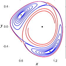
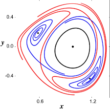
(a)	(b)
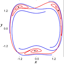
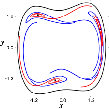
(c)	(d)

Fig. 6: Behavior of invariant curves of the Poincaré map for Eq. (2) at $\varepsilon=0.1$ and $p_{1}=1,p_{2}=-0.1,p_{3}=0.5,p_{4}=2.5$ (a); $p_{1}=1,p_{2}=-0.02,p_{3}=0.5,p_{4}=2.5$ (b); $p_{1}=1,p_{2}=0.03,p_{3}=1,p_{4}=3.36$ (c); $p_{1}=1,p_{2}=0.03,p_{3}=1,p_{4}=3$ (d).

Note that the fixed and periodic points in resonance zones correspond to resonance periodic solutions of period $2\pi p/p_{4}$ in the initial equation, and the closed invariant curves to quasiperiodic (double-frequency) solutions (two-dimensional tori).

4 On global behavior of solutions outside the neighborhood of “figure-eight”

The resonance levels corresponding to the limit cycles in the autonomous equation ($p_{3}=0$ in Eq. (2)) are splittable as $B_{j}(I_{pq})=0$, $j=1,2$ for these levels. According to Sec. 2, the number of such levels in each domain $G_{1}^{\pm},G_{2}$ is no more than two. Let us remove from these domains the neighborhoods of such levels and designate the remaining domains without the neighborhood of “figure-eight” by $V$. Using the results obtained in Morozov, [1998] and Eqs. (15), (18), (20) and (24), we obtain the following theorem.

Theorem 4.1.

There are only finitely many splittable resonance levels in $V$.

It follows from this theorem that for relatively small $\varepsilon>0$ the neighborhoods of splittable resonance levels do not intersect. This allows us to speak about the global behavior of solutions in the considered cells. According to Morozov, [1998], the separatrices of saddle periodic solutions lying at different resonance levels intersect, causing the formation of heteroclinic structures and a complicated geometry of the attraction domains of stable periodic solutions.

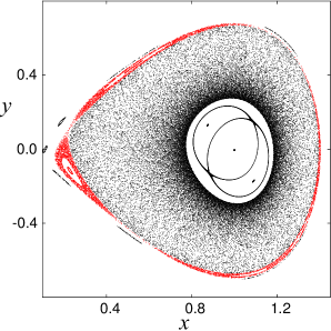
(a)	(b)

Fig. 7: Behavior of the trajectories of the Poincaré map for Eq. (2) in the case of two impassable resonances with $p=2$ and $p=3$ in domain $G_{1}^{+}$ (a), and a fragment of this domain (b). Here, $\varepsilon=0.01$, $p_{1}=-0.221$, $p_{2}=1.22$, $p_{3}=1$, $p_{4}=2.782$.

Consider as an example of the illustration of global behavior of solutions, a cell inside the right loop. Let the perturbed autonomous equation have two limit cycles in this cell (domain $D_{12}$ in the bifurcation diagram) and $\rho=\rho^{(1)}$, $\rho=\rho^{(2)}$ be simple roots of the Poincaré–Pontryagin function $B_{1}^{+}(\rho)$ in domain $G_{1}^{+}$.

Let us fix the parameter $p_{2}=1.22$ and find the values of the parameters $p_{1}$, $p_{4}$ at which the cycle $\rho=\rho^{(1)}$ coincides with the resonance level $I=I_{21}$, and the cycle $\rho=\rho^{(2)}$ with the level $I=I_{31}$. From the resonance condition (7) we have $p_{4}=2\omega(\rho^{(1)},p_{1})=3\omega(\rho^{(2)},p_{1})$. From this relation and the equations defining the limit cycles $B_{1}^{+}(\rho^{(1)},p_{1})=0$, $B_{1}^{+}(\rho^{(2)},p_{1})=0$, we find $p_{1}\approx-0.221$, $\rho^{(1)}\approx 0.45$, $\rho^{(2)}\approx 0.98$. Then, at $p_{4}\approx 2.782$ we will have impassable resonance zones. There exists in the initial equation a stable periodic solution of period $6\pi/p_{4}$ (stable periodic points of period-3 in the red zone in Fig. 7(a)) and an unstable periodic solution of period $4\pi/p_{4}$ (unstable periodic points of period-2 in the white zone in Fig. 7(a)). All the other resonance levels between the above ones will be passable. Between the resonance zones, trajectories fill the cell under consideration (see Fig. 7(a); actually, these trajectories are slowly spiraling and tend to stable periodic points of period-3 as $t\to\infty$). A higher-order partially passable resonance can be seen near the unperturbed separatrix loop in Fig. 7(a). A magnified fragment with a trajectory inside the resonance zone with $p=2$ is presented in Fig. 7(b), where one can see passable resonances. Passable resonances were also observed between the resonance zones with $p=2$ and $p=3$.

The behavior of the invariant curves of the Poincaré map in the neighborhood of the impassable resonance zone with $p=2$ is shown in more detail in Fig. 6(a).

5 Analysis of the behavior of solutions in the small neighborhood of “figure-eight”

The unperturbed equation $\ddot{x}-x+x^{3}=0$ has a right loop $\Gamma^{r}=\Gamma^{r}_{s}\bigcup\Gamma^{r}_{u}$ of saddle separatrix $O(0,0)$ and the left loop $\Gamma^{l}=\Gamma^{l}_{s}\bigcup\Gamma^{l}_{u}$ (Fig. 1).

It is known that under the action of perturbations, the separatrices of the fixed saddle point of the Poincaré map may intersect forming homoclinic structures of two types: 1) $\Gamma^{r}_{s}\bigcap\Gamma^{r}_{u}\neq\oslash$ and/or $\Gamma^{l}_{s}\bigcap\Gamma^{l}_{u}\neq\oslash$; 2) $\Gamma^{r}_{u}\bigcap\Gamma^{l}_{s}\neq\oslash$ or $\Gamma^{r}_{s}\bigcap\Gamma^{l}_{u}\neq\oslash$, when $p_{2}\neq 0$.

Existence of a homoclinic structure results in complicated behavior of solutions in its neighborhood or, in other words, in a nontrivial hyperbolic set Shil’nikov, [1967]. The problem of the existence of type 1) homoclinic structure is solved using the Melnikov formula Mel’nikov, [1963] $\Delta(t_{0})=\varepsilon\Delta_{1}(t_{0})+O(\varepsilon^{2})$, where $\Delta(t_{0})$ is the distance between the related branches of the separatrix into which the unperturbed separatrix splits. The substitution of $x=\xi+\varepsilon x_{1}(t)+O({\varepsilon}^{2})$, where

$$x_{1}(t)=-\frac{p_{3}}{1+{p_{4}}^{2}}\sin{(p_{4}t)},$$ (25)

in (2) yields the following equation

$$\ddot{\xi}-\xi+{\xi}^{3}=\varepsilon\left[(p_{1}+p_{2}\xi-{\xi}^{2})\dot{\xi}+\frac{3p_{3}}{1+{p_{4}}^{2}}{\xi}^{2}\sin{(p_{4}t)}\right].\\$$ (26)

Applying the Melnikov formula to this equation, we find

$$\Delta_{1}(t_{0})=2\left(\frac{2}{3}p_{1}\pm\frac{\pi}{8}\sqrt{2}p_{2}-\frac{8}{15}\right)+\frac{3\pi p_{4}}{2{\rm cosh}(\pi p_{4}/2)}p_{3}\cos{(p_{4}t_{0})}.$$ (27)

If $\Delta_{1}(t_{0})$ is an alternating function, which holds under the condition

$$|p_{3}|\ >p_{3}^{*}=\frac{4}{3}\left|\left(\frac{2}{3}p_{1}\pm\frac{\pi}{8}\sqrt{2}p_{2}-\frac{8}{15}\right)\frac{{\rm cosh}(\pi p_{4}/2)}{\pi p_{4}}\right|,$$ (28)

then there occurs transversal intersection of the stable and unstable manifolds of the fixed point.

If $\Delta_{1}(t_{0})$ is a constant-sign function, then the corresponding separatrix manifolds of the saddle fixed point do not intersect. However, if the value of $|p_{3}-p_{3}^{*}|$ is small enough, then, as follows from Gavrilov & Shil’nikov, [1972], Morozov, [1976], a nontrivial hyperbolic set exists in the neighborhood of “figure-eight”.

Under the condition

$$|p_{3}|\ =\ \frac{4}{3}\left|\left(\frac{2}{3}p_{1}\pm\frac{\pi}{8}\sqrt{2}p_{2}-\frac{8}{15}\right)\frac{{\rm cosh}{(\pi p_{4}/2)}}{\pi p_{4}}\right|$$ (29)

the corresponding separatrices of the fixed point $(0,0)$ are tangent to each other (to an accuracy of terms of order $\varepsilon^{2}$).

Making use of the Melnikov formula, it is easy to represent all possible cases of relative position of the separatrices as a result of splitting of the left or right separatrix loop. For example, for $p_{3}=0$, the condition

$$\frac{2}{3}p_{1}+\frac{\pi}{8}\sqrt{2}p_{2}-\frac{8}{15}=0$$

specifies the existence of the right separatrix loop. With allowance for external force, the outgoing and incoming separatrices intersect transversally, forming a homoclinic Poincaré structure. In this case, for the left separatrix loop we have

$$\Delta_{1}(t_{0})=-\frac{\pi}{2}\sqrt{2}p_{2}+\frac{3\pi p_{4}}{2{\rm cosh}{(\pi p_{4}/2)}}p_{3}\cos{(p_{4}t_{0})}.$$ (30)

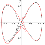
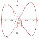
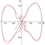
(a)	(b)	(c)

Fig. 8: Behavior of separatrices of the fixed point $(0,0)$ for Eq. (26) on the $(\xi=x,\dot{\xi}=y)$ plane at $\varepsilon=0.3$, $p_{1}=0.7551195621$, $p_{2}=0.053875454$, $p_{4}=4$ and $p_{3}=1.13$ (a), $p_{3}=1.7$ (b), $p_{3}=2.83$ (c).

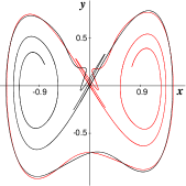
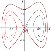
(a)	(b)

Fig. 9: Behavior of separatrices of the fixed point $(0,0)$ for Eq. (26) at $\varepsilon=0.1$, $p_{1}=0.78549$, $p_{3}=1.02$, $p_{4}=4$ and (a) $p_{2}=1.6$, (b) $p_{2}=-1.6$.

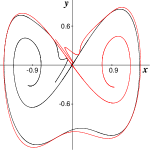
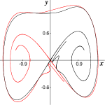
(a)	(b)
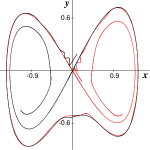
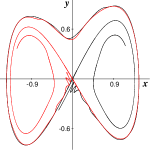
(c)	(d)

Fig. 10: Behavior of separatrices of the fixed point $(0,0)$ for Eq. (26) at $\varepsilon=0.175$, $p_{1}=0.78549$, $p_{3}=1.02$, $p_{4}=4$ and (a) $p_{2}=1.6$, (b) $p_{2}=-1.6$; $\varepsilon=0.175$, $p_{1}=0.7850145$, $p_{3}=0.57$, $p_{4}=4$, (c) $p_{2}=0.5$, (d) $p_{2}=-0.5$.

The separatrices of the fixed point $(0,0)$ of the Poincaré map on the $(\xi=x,\dot{\xi}=y)$ plane are shown in Fig.  8 for $\varepsilon=0.3$, $p_{1}=0.7551195621$, $p_{2}=0.053875454$, $p_{4}=4$ and $p_{3}=1.13$ (a), $p_{3}=1.7$ (b), and $p_{3}=2.83$ (c).

Note that for $p_{1}=0.8$, $p_{2}=0$, $p_{3}=0$ the unstable limit cycle in Eq. (2) coincides with “figure-eight”. Then, for small enough $p_{3}\neq 0$, the inverse Poincaré map has a quasiattractor.

When a perturbed autonomous equation has a “big” separatrix loop, the Melnikov formula does not hold for a nonautonomous equation. For this case, the separatrices of a fixed saddle point of the Poincaré map for Eq. (26) on the $(\xi=x,\dot{\xi}=y)$ plane are shown in Fig.  9 for $\varepsilon=0.1$, $p_{1}=0.78549$, $p_{3}=1.02$, $p_{4}=4$ and (a) $p_{2}=1.6$, (b) $p_{2}=-1.6$. There occurs transversal intersection of the corresponding separatrices ($\Gamma^{r}_{u}\bigcap\Gamma^{l}_{s}\neq\oslash$ in Fig. 9(a) and $\Gamma^{r}_{s}\bigcap\Gamma^{l}_{u}\neq\oslash$ in Fig. 9(b)). Also, homoclinic structures with tangency (Fig. 10) are possible at different values of the parameters.

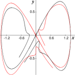
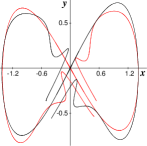
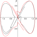
(a)	(b)	(c)
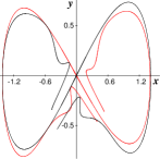
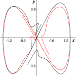
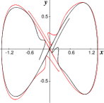
(d)	(e)	(f)
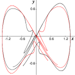
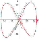
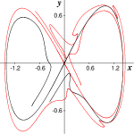
(g)	(h)	(i)
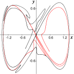
(j)

Fig. 11: Other homoclinic structures with tangency of stable and unstable separatrices of the fixed point $(0,0)$ for Eq. (26).

Figure 11 illustrates other homoclinic structures with tangency of stable and unstable separatrices of the fixed point $(0,0)$ for Eq. (26) at $\varepsilon=0.12$, $p_{4}=4$ for the following values of the parameters $p_{1}$, $p_{2}$, $p_{3}$: (a) $p_{1}=0.7$, $p_{2}=0.3$, $p_{3}=3$; (b) $p_{1}=0.86$, $p_{2}=0.2$, $p_{3}=4.55$; (c) $p_{1}=0.6$, $p_{2}=0.1$, $p_{3}=2.34$; (d) $p_{1}=0.86$, $p_{2}=0.25$, $p_{3}=2.96$; (e) $p_{1}=1$, $p_{2}=0.1$, $p_{3}=2.32$; (f) $p_{1}=0.7$, $p_{2}=0$, $p_{3}=2$; (g) $p_{1}=0.8$, $p_{2}=0.2$, $p_{3}=3.34$; (h) $p_{1}=0.9$, $p_{2}=0$, $p_{3}=1.98$; (i) $p_{1}=0.65$, $p_{2}=0.35$, $p_{3}=2.82$; (j) $p_{1}=0.9$, $p_{2}=0.3$, $p_{3}=2.97$.

6 Bifurcation diagrams

Using the WInSet and Maple 13 software, we constructed three bifurcation diagrams of the Poincaré map for Eq. (26) on the $(p_{2},p_{3})$ plane for fixed values of the parameters $\varepsilon$, $p_{1}$, and $p_{4}$. In the bifurcation curves, the corresponding separatrices of the fixed point (0,0) are tangent to each other. These curves separate domains with homoclinic structure on the plane of parameters $(p_{2},p_{3})$ (the stable and unstable separatrices of the saddle point (0,0) intersect transversally). The three bifurcation diagrams describe all possible cases of the relative position of separatrices of the fixed saddle point (0,0) for the Poincaré map.

The obtained bifurcation diagrams are symmetric to the $p_{3}$ axis. Let us set $p_{2}>0$ and consider in more detail each of the three bifurcation diagrams. By fixing $\varepsilon=0.12$, $p_{1}=0.78$, $p_{4}=4$, we obtain six bifurcation curves. Equations for the straight lines $M_{1}$, $M_{2}$, $M_{3}$ are found from (29). The other bifurcation curves $M_{4}$, $M_{5}$, $M_{6}$ are obtained numerically by means of the WInSet software. Each pair of lines $M_{2}$ and $M_{3}$, $M_{4}$ and $M_{5}$, $M_{5}$ and $M_{6}$ have exactly one common point on the $p_{2}$ axis. The first point ($p_{2}\approx 0.024$) corresponds to the right separatrix loop in the autonomous equation; the next two points ($p_{2}\approx 0.25838$ and $p_{2}\approx 1.0983$) correspond to the “big” separatrix loop in the autonomous equation. The intersection points of the lines $M_{2}$ and $M_{4}$, as well as of the lines $M_{1}$, $M_{3}$ and $M_{4}$ correspond to double homoclinic tangency. The obtained bifurcation curves are presented in Fig. 12.

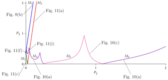
Fig. 12: Bifurcation diagram for the Poincaré map on the $(p_{2},p_{3})$ plane at $p_{1}=0.78$.

Setting $\varepsilon=0.12$, $p_{1}=0.8$, $p_{4}=4$, we obtain three bifurcation curves shown in Fig. 13. As the parameter $p_{1}$ changes from $0.78$ to $0.8$ the straight lines $M_{1}$ and $M_{2}$ in Fig.  12 approach each other and coincide at $p_{1}=0.8$. As a result we obtain a straight line $N_{1}$ with a new type of tangency – double homoclinic tangency. An equation for $N_{1}$ is found from (29). The lines $N_{2}$ and $N_{3}$ obtained numerically have one common point ($p_{2}\approx 1.788$, $p_{3}=0$) corresponding to the “big” separatrix loop in the autonomous equation.

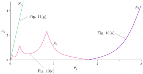
Fig. 13: Bifurcation diagram for the Poincaré map on the $(p_{2},p_{3})$ plane at $p_{1}=0.8$.

Setting $\varepsilon=0.12$, $p_{1}=0.82$, $p_{4}=4$, we obtain five bifurcation curves plotted in Fig. 14. Equations for the straight lines $R_{1},R_{2},R_{3}$ are found from (29). The other bifurcation lines $R_{4},R_{5}$ are obtained numerically using the WInSet software. The intersection point of the curves $R_{4}$ and $R_{5}$ ($p_{2}\approx 2.28515$, $p_{3}=0$) corresponds to the “big” separatrix loop in the autonomous equation. The intersection points of $R_{2}$ and $R_{4}$ and of $R_{1}$, $R_{3}$ and $R_{4}$ give double homoclinic tangencies.

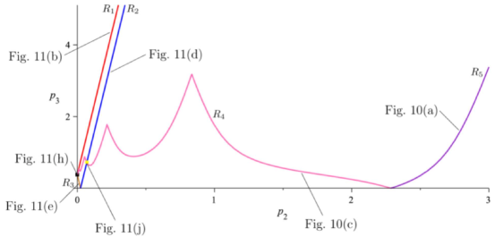
Fig. 14: Bifurcation diagram for the Poincaré map on the $(p_{2},p_{3})$ plane at $p_{1}=0.82$.

Each of the three bifurcation diagrams has domains with homoclinic structure and a nonsmooth boundary. This phenomenon was explained in ample detail in the work Gonchenko et al., [2013].

7 Conclusion

The problem of time-periodic perturbations of two-dimensional Hamiltonian systems with a saddle and two separatrix loops in the form of “figure-eight” is a challenging problem for the theory of bifurcations. Bifurcations in the neighborhood of “figure-eight” for the case of an unperturbed autonomous system with a nonzero saddle value were recently considered in Gonchenko et al., [2013]. This problem for the case of a zero saddle value has not been fully understood yet. The asymmetric Duffing–Van-der-Pol equation (2) studied in the present work is a good model for solution of this problem.

Despite its fundamental role in the theory of differential equations, the theory of bifurcations, and the theory of oscillations, Eq. (2) has not been studied thus far for the case when $p_{2}\neq 0$. We have solved the problem of limit cycles in the autonomous case. For the nonautonomous case, we have found resonance zone structures and global behavior of solutions in the cells separated from unperturbed separatrices. Different resonance periodic solutions and two-dimensional invariant tori have also been found. The problem of the existence of homoclinic structures in the neighborhood of unperturbed separatrices (in the neighborhood of “figure-eight”) has been solved. All possible cases of relative position of the separatrices of a trivial fixed saddle point for the Poincaré map have been revealed. Three bifurcation diagrams for the Poincaré map on the $(p_{2},p_{3})$ plane separating domains of existence of different homoclinic structures have been constructed. The results obtained for the separatrix tangency illustrate many specific features found in Gonchenko et al., [2013] for two-parametric families of maps in the neighborhood of “figure-eight” with nonzero saddle value.

Note that some of the problems associated with the presence of homoclinic structures remain open. For example, one such problem is to study fractal properties of attraction basin boundaries for stable periodic regimes in the considered equation.

8 Acknowledgments

We dedicate this paper to the memory of the outstanding scientist Leonid P. Shil’nikov, the pioneer of homoclinic bifurcation theory. The authors are grateful to M.I. Malkin for helpful discussions and comments. This work was partially supported by the Russian Science Foundation, grant No 14-41-0044.

References

- Arnold, [1978] Arnold, V.I. [1978] “Additional Chapters of the Theory of Ordinary Differential Equations”, Nauka, Moscow (Russian).
- Bautin, [1975] Bautin, A.N. [1975] “Qualitative study of one nonlinear system”, Prikl. Mat. i Mekh. (Russian), vol. 39, no. 4, pp. 633–641.
- Bautin & Leontovich, [1976] Bautin, N.N. & Leontovich, E.A. [1976] “Methods and Techniques of Qualitative Investigation of Dynamical Systems on a Plane”, Nauka, Moscow (Russian).
- Gavrilov & Shil’nikov, [1972] Gavrilov, N.K. & Shil’nikov, L.P. [1972] “On three dimensional systems close to systems with nonrough homoclinical curve”, Mat. Sb. (Russian), vol. 88, no. 4, pp. 475–492. (Eng. ver.: Mathematics of the USSR-Sbornik, vol. 17, no. 4, pp. 467–485).
- Gonchenko et al., [2013] Gonchenko, S.V., Simo, C. & Vieiro, A. [2013] “Richness of dynamics and global bifurcations in systems with a homoclinic figure-eight”, Nonlinearity, vol. 26, no. 3, pp. 621–678.
- Guckenheimer & Holmes, [1983] Guckenheimer, J. & Holmes, Ph. [1983] “Nonlinear Oscillations, Dynamical Systems and Bifurcations of Vector Fields”.–N.Y.–Berlin–Heidelberg–Tokyo: Springer.
- Kostromina & Morozov, [2012] Kostromina, O.S. & Morozov, A.D. [2012] “On limit cycles in the asymmetric Duffing–Van-der-Pol equation”, Nizhny Novgorod: Vestnik Nizhegorodskogo Universiteta (Russian), no. 1, pp. 115–121.
- Litvak-Hinenzon & Rom-Kedar, [1997] Litvak-Hinenzon, A. & Rom-Kedar, V. [1997] “Symmetry-breaking perturbations and strange attractors”, Phys. Rev. E., vol. 55, no. 5, pp. 4964–4978.
- Mel’nikov, [1963] Mel’nikov, V.K. [1963] “On stability of a center under periodic in time perturbations”, Works of Moscow Math. Socity (Russian), vol. 12, pp. 3–53.
- Morozov, [1973] Morozov, A.D. [1973] “To the problem on total qualitative investigation of Duffing equation”, Journal of Numerical Math. and Math. Phis. (Russian), vol. 13, no. 5, pp. 1134–1152.
- Morozov & Shil’nikov, [1975] Morozov, A.D. & Shil’nikov, L.P. [1975] “To mathematical theory of oscillatory synchronization”, Dokl. Akad. Nauk SSSR (Russian), vol. 223, no. 6, pp. 1340–1343.
- Morozov & Shil’nikov, [1983] Morozov, A.D. & Shil’nikov, L.P. [1983] “On nonconservative periodic systems similar to two-dimensional Hamiltonian ones”, Prikl. Mat. i Mekh. (Russian), vol. 47, no. 3, pp. 385–394.
- Morozov, [1976] Morozov, A.D. [1976] “On total qualitative investigation of the Duffing equation”, Differentsial’nye Uravnenia (Russian), vol. 12, no. 2, pp. 241–245.
- Morozov, [1993] Morozov, A.D. [1993] “On the global behavior of self-oscillatory systems”, Int. J. of Bifurcation and Chaos, vol. 3, no. 1, pp. 195–200.
- Morozov & Fedorov, [1976] Morozov, A.D. & Fedorov, E.L. [1979] “On self-oscillatories in two dimensional dynamical systems”, Prikl. Mat. i Mekh. (Russian), vol. 43, no. 4, pp. 602–611.
- Morozov, [1998] Morozov, A.D. [1998] “Quasi-conservative systems: cycles, resonances and chaos”.–Singapore: World Sci, in ser. Nonlinear Science, ser. A, vol. 30, 325 p.
- Morozov et al., [1999] Morozov, A.D., Dragunov, T.N., Boykova S.A. & Malysheva, O.V. [1999] “Invariant Sets for Windows: Resonance Structures, Attractors, Fractals and Patterns”, World Scientific Ser. on Nonlinear Science, Series A, vol. 37, Series Ed. Leon Chua.
- Morozov & Dragunov, [2003] Morozov, A.D. & Dragunov, T.N. [2003] “Visualization and analysis of invariant sets of dynamical systems”, Moscow–Izhevsk: Publishing house of the Institute of Computer Research (Russian).
- Shil’nikov, [1967] Shil’nikov, L.P. [1967] “On a Poincare–Birkhoff problem”, Mat. Sb. (Russian), vol. 74(116), no. 3, pp. 378–397. (Eng. ver.: Mathematics of the USSR-Sbornik, vol. 3, no. 3, pp. 353–371).
- Wiggins, [1990] Wiggins, S. [1990] “Introduction to Applied Nonlinear Dynamical Systems and Chaos”.–Springer–Berlin.