Ultrathin fibres from electrospinning experiments under driven fast-oscillating perturbations

Abstract

The effects of a driven fast-oscillating spinneret on the bending instability of electrified jets, leading to the formation of spiral structures in electrospinning experiments with charged polymers, are explored by means of extensive computer simulations. It is found that the morphology of the spirals can be placed in direct correspondence with the oscillation frequency and amplitude. In particular, by increasing the oscillation amplitude and frequency, thinner fibres can be extracted by the same polymer material, thereby opening design scenarios in electrospinning experiments.

I Introduction

The dynamics of charged polymer jets under the effect of an external electrostatic field stands out as major challenge in non-equilibrium thermodynamics, with numerous applications in micro and nano-engineering and life sciences as well  Yarin (1993); Reneker et al. (2000); Yarin et al. (2001); Loscertales et al. (2002); Dzenis (2004); Helgeson et al. (2008); Thompson et al. (2007); Grafahrend et al. (2011); Greenfeld et al. (2012); Onses et al. (2013); Min et al. (2013). Indeed, charged liquid jets may develop several types of instabilities depending on the relative strength of the various forces acting upon them, primarily electrostatic Coulomb self-repulsion, viscoelastic drag and surface tension effects. Among others, one should mention bending and “whipping” instabilities, the latter consisting of fast large-scale lashes, resembling the action of a whip. These instabilities are central to the manufacturing process known as electrospinning  Regev et al. (2013); Nakano et al. (2012); Greiner and Wendorff (2007); Fridrikh et al. (2003); Camposeo et al. (2013); Pisignano (2013). Some of them were analysed in the late sixties by G.I. Taylor Taylor (1969). In the subsequent years, it became clear that the driver of such instabilities is the Coulomb self-repulsion, as it can be inferred by simply observing that any off-axis perturbation of a collinear set of equal-sign charges would only grow under the effect of Coulomb repulsion Reneker et al. (2000); Marin et al. (2008).

In the electrospinning process, ultrathin fibres, with diameters in the range of hundreds of nanometres and below, are produced out of charged polymer jets. In addition to its fundamental importance in the fields of soft matter physics and fluid dynamics, electrospinning is raising a continuously increasing interest due to its widespread application fields. For this reason, nowadays this technique is an excellent example of how applied physics impacts on engineering and materials science. For example, recently electrospun nanofibres and nanowires have been used for realizing organic field-effects transistors  Liu et al. (2005); Min et al. (2013), whose fabrication benefits from the concomitant high spatial resolution of active channels, large-area deposition, and frequently improved charge carrier mobility, which is highly relevant for nanoelectronics. Other important applications are in the field of photonics  Camposeo et al. (2013), and include solid-state organic lasers  Persano et al. (2014), light-emitting devices  Moran-Mirabal et al. (2007); Vohra et al. (2011), and active nanomaterials featuring high internal orientational order of embedded chromophores, thus exhibiting polarized infrared, Raman  Kakade et al. (2007); Pagliara et al. (2011); Richard-Lacroix and Pellerin (2012) and emission spectra  Pagliara et al. (2009). Electrohydrodynamics jet printing has been recently applied in order to control the hierarchical self-assembly of patterns in deposited block-copolymer films  Onses et al. (2013), with important applications in nanomanufacturing and surface engineering. Electrostatic spinning is also a tool for medical sciences and regenerative medicine, e.g. for the construction of complex scaffolding necessary for tissue growth  Grafahrend et al. (2011); Xie et al. (2009), or for the accurate encapsulation of solutions into monodisperse drops  Loscertales et al. (2002). In general electrospinning is an excellent technique to transfer to a macroscopic composite material the properties of complex polymer solutions Dzenis (2004), which can have a direct impact on the mechanical properties of resulting nanofibers  Arinstein et al. (2007). In this respect, an aspect which is particularly critical is that fibres can reach a diameter in the nanometre scale. Electrospinning can reach such scales, especially thanks to the occurrence of instabilities that drive the system to extend on the plane orthogonal to the jet axis Yarin (1993); Reneker et al. (2000); Yarin et al. (2001); Helgeson et al. (2008); Thompson et al. (2007); Greenfeld et al. (2012). In such experiments, a droplet of charged polymer solution is injected from a nozzle at one end of the apparatus (spinneret), then it is elongated and the resulting collinear jet moves away from the droplet under the effect of an externally applied electrostatic field. Such collinear configuration is however unstable against off-axis perturbations, as one can readily realize by inspecting the effect of Coulomb repulsion on different portions of the jet. The resulting bending instability often gives rise to three dimensional helicoidal structures (spirals). Due to polymer mass conservation, the spiral structures get thinner and thinner as they proceed downwards, until they hit a collecting plate at the bottom. Based on the above, it is clear that an accurate control of the effects of the bending and whipping instabilities on the morphological features of the resulting spirals is key to an efficient design of the electrospinning process. The fundamental physics of the electrospinning process is governed by the competition between Coulomb repulsion and the stabilizing effects of viscoelastic drag and surface tension. Since the timespan of the entire process is comparable with the relaxation time of the polymer material, electrospinning qualifies as a strongly off-equilibrium process.

A number of papers have been dealing with the theory of the electrospinning process Hohman et al. (2001a, b); Reneker et al. (2000); Yarin (1993); Greenfeld et al. (2011); Fridrikh et al. (2003); Pontrelli et al. (2014). Broadly speaking, these models fall within two general classes: continuum and discrete. The former treat the polymer jet as a charged fluid, obeying the equations of continuum mechanics, while the latter represent the jet as a discrete collection of charged particles (beads), subject to four type of interactions: Coulomb repulsion, viscoelastic drag, curvature-driven surface tension and, finally, the external electric field.

However, due to the complexity of the resulting dynamics and to the large number of experimental parameters involved in the process (related to solution, field and environmental properties), electrified jets are still treated by empirical approaches. For instance, either near-field techniques have been proposed to reduce instabilities Sun et al. (2006); Bisht et al. (2011), or the effect of the different parameters on the resulting nanofibre properties and radius have been determined empirically through systematic campaigns Thompson et al. (2007); Pai et al. (2011). Indeed, to date most investigations on electrospinning have been focussing on the experimental exploration of the various type of polymers that are liable to be electrospun into fibres, as well as on the processing/properties of the spun fibres.

In addition, the dynamics of the jet is also sensitive to random external disturbances (noise), and particularly to erratic oscillations of the injection apparatus and of ambient atmosphere, which could act as hidden variables critically affecting the reliability of the process. In the sequel, we shall consider such fast mechanical oscillations of the spinneret as a driving perturbation, whose amplitude and frequency can be fine-tuned in order to minimize the thickness of the electrospun fibre. This portrays an angle of investigation of the electrospinning process that we proceed to investigate, on a systematic basis in this paper. In particular, it is found that either increasing the perturbation amplitude, frequency, or both can lead to obtain thinner jets, hence thinner fibres in the end. More precisely, by increasing the perturbation amplitude, spirals are seen to open up into a broader cone envelope, hence resulting into thinner fibres. By increasing the perturbation frequency, on the other hand, the spirals are developed with a shorter pitch, resulting again in thinner fibres at the collecting plate. To highlight the potential of driving the injected fluid to produce thinner fibres in practice, we point out that increasing the perturbation amplitudes, from say $1.6\;10^{-4}\;\text{cm}$ to $1.6\;10^{-3}\;\text{cm}$, while keeping the other process parameters unchanged, leads to a three-fold reduction of the resulting fibre thickness for polyethylene oxide and other plastic materials. Similarly, varying the perturbation frequency from $10^{5}\;\text{s}^{-1}$ to $10^{6}\;\text{s}^{-1}$ determines a three-fold fibre thickness decrease.

II Mathematical model

The mathematical model used in this paper closely follows the one given in the pioneering work by Reneker and coworkers  Reneker et al. (2000), namely the jet is described by a sequence of discrete charged particles (beads), obeying Maxwell fluid mechanics under the effects of the four forces described above. The polymer jet is represented by means of a Maxwellian liquid, coarse-grained into a viscoelastic bead-spring model with a charge associated to each bead. This representation is justified by the earlier work of Yarin Yarin (1990, 1993). In Fig. 1 we show how the experimental set-up looks like. On the top of the figure there is the pendant drop, which is dangling from a pipette or from a syringe. Between the pipette placed along the $Z$-axis at a height $h$ and the collecting plane (not visible in the figure) at $Z=0$, the electric field $V_{0}/h$ is applied downwards along the $Z$ direction.

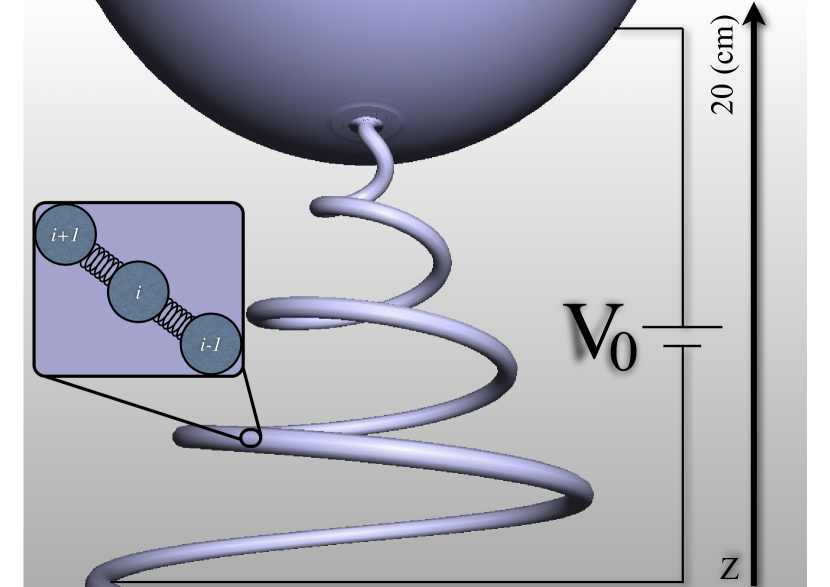
Figure 1: Schematic representation of the model for the polymer jet. The jet is generated from the pendant drop on the top of the figure upon application of the external field $V_{0}/h$. The jet is then represented at a microscopic level as a bead-spring chain. Each bead is charged while the connecting springs are calculated by solving the associated polymer stress equations at each molecular dynamics time step.

We shall consider the following experimental parameters: $a_{0}$ is the initial cross-section radius of the electrified jet, $e$ is the charge per particle, $G$ is the elastic modulus, $h$ is the distance from the drop to the collector, $m$ is the mass of each particle, $\mu$ is the dynamic viscosity, $\theta=\mu/G$ is the relaxation time, $\alpha$ is the surface tension, and $V_{0}$ is the voltage applied between the drop and the grounded collector plate. In what follows we will use Gaussian units for charges (CGS units). In Fig. 1, the spring represents the stress $\sigma$ in the Maxwellian fluid and it is determined by the stress equation between each consecutive pairs of beads. The coupled system of Newton equations for the beads and the associated stress equation reads as follow:

$$\begin{cases}&m\frac{d^{2}\vec{R_{i}}}{dt^{2}}=\vec{F_{i}}\\ &\frac{d\sigma_{i}}{dt}=\frac{1}{l_{i}}\frac{dl_{i}}{dt}-\sigma_{i},\end{cases}$$ (1)

where $\vec{R_{i}}=\left(X_{i},Y_{i},Z_{i}\right)$ is the position vector of the i-th bead, $l_{i}=\left[{\Delta X_{i}}^{2}+{\Delta Y_{i}}^{2}+{\Delta Z_{i}}^{2}\right]^{1/2}$ is the distance between two bonded beads. Space and time units have been chosen as $t=t_{\text{phys}}/\theta$ and $l=l_{\text{phys}}/L$, where $L=(e^{2}/\pi a^{2}_{0}G)^{1/2}$. In the sequel, the superscript (subscript) U (respectively D), will refer to the “up” $(i+1)$ and “down” $(i-1)$ beads, respectively, where $i$ is the bead index. The coupling between the equations Eq. 1 takes place through the net viscoelastic force $\vec{F}_{\texttt{VE}}$ acting on the bead $i$, which is given by:

$$\vec{F}_{\texttt{VE}}=F_{ve} \left[\left(a^{2}_{U}\sigma^{U}_{i}\frac{X_{i+1}-X_{i}}{l^{U}_{i}}-a^{2}_{D}\sigma^{D}_{i}\frac{X_{i}-X_{i-1}}{l^{D}_{i}}\right)\vec{i}\right.$$ (2)

$$+\left(a^{2}_{U}\sigma^{U}_{i}\frac{Y_{i+1}-Y_{i}}{l^{U}_{i}}-a^{2}_{D}\sigma^{D}_{i}\frac{Y_{i}-Y_{i-1}}{l^{D}_{i}}\right)\vec{j}$$

$$\left.+\left(a^{2}_{U}\sigma^{U}_{i}\frac{Z_{i+1}-Z_{i}}{l^{U}_{i}}-a^{2}_{D}\sigma^{D}_{i}\frac{Z_{i}-Z_{i-1}}{l^{D}_{i}}\right)\vec{k}\right]$$

where in reduced units one has $a^{2}_{U}=1/l^{U}_{i}$ and $a^{2}_{D}=1/l^{D}_{i}$. Besides the viscoelastic force $\vec{F}_{\texttt{VE}}$, each bead is subject to three additional forces, namely: the driving force $\vec{F_{0}}$ of the external field $\vec{V_{0}}$, acting between the drop and the collection plate, the bead-bead Coulomb interaction $\vec{F}_{\texttt{Coul}}$, and the surface tension force $\vec{F}_{\texttt{Cap}}$, which acts as an effective bending rigidity penalising curved jet shapes. These forces read as follows:

$$\vec{F_{0}} = -\frac{e\mu^{2}|\vec{V_{0}}|}{hLmG^{2}}\vec{k}$$

$$\vec{F}_{\texttt{Coul}} = Q\sum_{j}\left(\frac{X_{i}-X_{j}}{R_{ij}^{3}}\;\vec{i}+\frac{Y_{i}-Y_{j}}{R_{ij}^{3}}\;\vec{j}+\frac{Z_{i}-zß_{j}}{R_{ij}^{3}}\;\vec{k}\right)$$

$$\vec{F}_{\texttt{Cap}} = A\;k_{i}\left(-X_{i}\frac{(a_{U}+a_{D})^{2}}{4\sqrt{X^{2}_{i}+Y^{2}_{i}}}\;\vec{i}-Y_{i}\frac{(a_{U}+a_{D})^{2}}{4\sqrt{X^{2}_{i}+Y^{2}_{i}}}\;\vec{j}\right)$$ (3)

where $F_{ve}\equiv Q=\frac{\pi a^{2}_{0}\mu^{2}}{LmG}$, $A=\frac{\pi\alpha a^{2}_{0}\mu^{2}}{mL^{2}G^{2}}$, $R_{ij}$ is the distance between two beads, and $k_{i}$ is the local curvature, defined as the radius of the circle going through the points $i+1$, $i$ and $i-1$. It is important to stress that the model also assumes that the fluid is incompressible, which results in the mass conservation law:

$$\pi a^{2}l=\pi a_{0}^{2}l_{0}$$ (4)

This determines the fibre thickness $a$ as a function of the elongation $l$. At each time step, we first integrate the above stress equations Eq. 1, and then we use the updated stress terms to integrate the equations of motion which, in turn, are solved with a simple velocity Verlet integration scheme with the same integration time step $\Delta t$ used for the stress equation.

III Numerical integration scheme

We solve Eq. 1 in an equivalent but numerically more convenient form:

$$\frac{d\left(e^{t}\sigma\right)}{dt}=e^{t}\left(\frac{1}{l}\frac{dl}{dt}\right)$$ (5)

using the forward Euler discrete integration scheme with an integration step $\Delta t$:

$$e^{t}\;\sigma(t)-e^{t-\Delta t}\;\sigma(t-\Delta t)=\Delta t\;e^{t}\left(\frac{1}{l(t)}\frac{l(t)-l(t-\Delta t)}{\Delta t}\right)$$ (6)

which leads to the explicit time marching scheme

$$\sigma(t)=e^{-\Delta t}\;\sigma(t-\Delta t)+\frac{l(t)-l(t-\Delta t)}{l(t)}$$ (7)

The Euler integration is coupled to a Verlet time integration scheme as follows, given the initial conditions at $t=-\Delta t$ and at $t=0$ :

1. Stress at time $t$: $\sigma(t-\Delta t)\rightarrow\sigma(t)$ from Eq. 7;

2. Forces at time $t$: $\vec{F}(t)=\vec{F}_{\texttt{VE}}+\vec{F}_{\texttt{Coul}}+\vec{F}_{\texttt{Cap}}+\vec{F_{0}}$;

3. Positions at time $t+\Delta t$: $\vec{r}(t+\Delta t)=2\vec{r}(t)-\vec{r}(t-\Delta t)+\vec{F}(t)\Delta t^{2}$;

4. Velocities at time $t+\Delta t$: $\vec{v}(t+\Delta t)=(\vec{r}(t+\Delta t)-\vec{r}(t-\Delta t))/(2\Delta t)$.

We wish to point out that the $1/r^{2}$ Coulomb singularity needs to be handled with great care, especially at the injection stage, where beads are inserted at a mutual distance shorter than their linear size. This imposes very small time-steps, of the order of $10^{-8}\mu/G$.

The effect of mechanical oscillations is mimicked by injecting the tail bead $i=N(t);\vec{V}^{i}_{\text{Init}}=0$, $N(t)$ being the number of beads in the chain at time $t$, at an off-axis position given by:

$$X_{N}=N_{s}L\cos(\Omega t)$$ (8)

$$Y_{N}=N_{s}L\sin(\Omega t)$$ (9)

$$Z_{N}=h-L_{ins}$$ (10)

where $L_{ins}=h/I_{F}$ is the insertion length and $I_{F}$ the insertion factor, $h$ the vertical size of the apparatus, typically $I_{F}=50000$, $N_{s}\ll 1$ is the amplitude and $\Omega$ is the frequency of the dynamical perturbation. In the sequel we shall refer to $N_{s}$ as to the noise strength. We remind that the insertion algorithm proceeds by inserting the $N$-th bead (polymer jet tail) once the distance between the $(N-1)$-th bead and the pendant drop at $Z=h$ exceeds the insertion distance, $L_{ins}=h/I_{F}$. Thus, the jet is represented by a bead chain with the tail, $i=N$, at the spinneret and the head, $i=1$, proceeding downwards to the collector. The idea behind this model Reneker et al. (2000) is that, by choosing $\Omega\gg 1$, the above algorithm would generate a quasi-random sequence of initial slopes of the polymer bead chain, whose envelope defines a conical surface known as the Taylor cone. In this work, however, the expression (8-9) stands for a deterministic, controlled source of fast oscillations, whose amplitude and frequencies can be fine-tuned to design thinner fibres. To quantitatively explore this idea, we have run simulations with several values of the perturbation strength $N_{s}$ and perturbation frequency $\Omega$.

Boundary conditions are imposed at the two ends of the jet: at $Z=h$ (top) and at the collecting plate $Z=0$ (bottom). The latter is treated as an impenetrable plane, at which the Coulomb forces are set to zero and the $Z$ component of the bead position is not allowed to take negative values. The top boundary condition is such that the $X$ and $Y$ components of the forces acting on the pendant drop are set to zero, while the $Z$ component must be non positive, i.e. point downwards.

In what follows, we will use the scheme above to solve the time development of the jet with a reference set of parameters pretty close, yet not exactly equal to the one given in the original paper by Reneker et al. Reneker et al. (2000) as presented in Table LABEL:tab:Real_Values. For the case in point $L=0.32$ cm and $\theta=0.01$ s. The resulting dimensionless parameters are given in the right panel of Table I, where $Q$, $F_{ve}$ and $A$, are the strength of Coulomb repulsion, viscoelastic forces and surface tension, respectively, $K_{s}=\Omega\;\theta$ is the injection frequency, $H=h/L$ and $\vec{F_{0}}$ is the scaled force resulting form the external field, all in dimensionless units.

Table 1: Simulation parameters obtained from the experimental data in the paper of Reneker et al. Reneker et al. (2000)

Experimental Parameters

Simulation Parameters

$\displaystyle\alpha$ $\displaystyle=$ $\displaystyle 700\,\text{g}/\text{s}^{2}$ $\displaystyle a_{0}$ $\displaystyle=$ $\displaystyle 1.5\;10^{-2}\,\text{cm}$ $\displaystyle e$ $\displaystyle=$ $\displaystyle 8.48\,\frac{g^{1/2}\text{cm}^{3/2}}{\text{s}}$ $\displaystyle\theta$ $\displaystyle=$ $\displaystyle 0.01\,\text{s}$ $\displaystyle G$ $\displaystyle=$ $\displaystyle 10^{6}\,\frac{\text{g}}{\text{cm}\;\text{s}^{2}}$ $\displaystyle h$ $\displaystyle=$ $\displaystyle 20\;\text{cm}$ $\displaystyle m$ $\displaystyle=$ $\displaystyle 2.83\;10^{-6}\;\text{g}$ $\displaystyle\mu$ $\displaystyle=$ $\displaystyle 10^{4}\;\frac{\text{g}}{cm\;s}$ $\displaystyle V_{0}$ $\displaystyle=$ $\displaystyle 10^{4}\;\text{V}$ $\displaystyle\Omega$ $\displaystyle=$ $\displaystyle 10^{4}\;\text{s}^{-1}$

$\displaystyle Q$ $\displaystyle\equiv$ $\displaystyle F_{ve}=78309.8\;\text{(Eq.\ref{forces})}$ $\displaystyle F_{0}$ $\displaystyle=$ $\displaystyle 157.9\;\text{(Eq.\ref{forces})}$ $\displaystyle A$ $\displaystyle=$ $\displaystyle 171.9\;\text{(Eq.\ref{forces})}$ $\displaystyle K_{s}$ $\displaystyle=$ $\displaystyle 100$ $\displaystyle H$ $\displaystyle=$ $\displaystyle 62.8$

IV Results and Discussion

In Fig. 2(a), we show a typical shape of the jet at the end of a simulation, lasting about $10^{6}$ time steps. As one can appreciate, spirals show from three to about ten turns over distances of a few centimetres, which is consistent with experimental observation Reneker and Yarin (2008); Bhattacharjee and Rutledge (2011). While we cannot rule out the possibility that kinematic effects play a major role in the spiral formation, we must observe that the morphology of the spiral appears highly dependent on the choice of the initial conditions and forcing parameters. In this respect, even the kinematics alone may not be trivial at all. We also considered a scenario whereby the perturbation is not applied on the $XY$-plane, but only along the $X$-axis. Since the component of the force along the $Y$-axis is always zero, the jet does not develop any component in the $YZ$-plane, resulting in a flat sinusoidal profile in the $XZ$-plane (Fig. 2(b)). Also these classes of planar spirals are frequently observed in experiments, and not explored in previous theoretical papers. The extreme variability of experimentally observed spirals can therefore be accounted for by considering the oscillating perturbation as an independent variable affecting the resulting dynamics of the electrified jets.

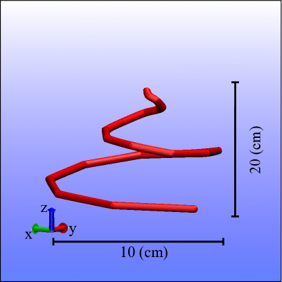
(a)

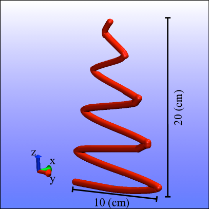
(b)

Figure 2: Final configuration of the filament in the case of a circular driving perturbation (a) and a linear one (b). Parameters used for the simulations are $V_{0}=10^{4}$ V, $\Omega=5\;10^{5}\;\text{s}^{-1}$, $N_{s}=10^{-3}$ and the total spinneret-collector distance $h=20$ cm, which resulted in the rescaled quantities $L=0.32$ $Q=F_{ve}=78309.8$, $F_{0}=157.9$, $A=171.9$, $H=62.8$. The linear dimensions are depicted in the figure and correspond to the following range of the axes: $X\in[-5,5]$ cm, $Y\in[-5,5]$ cm and $Z\in[0,20]$ cm.

IV.1 Effect of the perturbation amplitude

One of the environmental parameters of the model is the amplitude of the noise on the pendant drop, related to the vibrations that affect the experiment at the microscale. In the paper of Reneker et al. Reneker et al. (2000), the noise amplitude was kept fixed to $N_{s}=10^{-3}$. In Fig. 3 we show the comparison between the results in the amplitude range $N_{s}\in\left[5\;10^{-4},\ldots,5\;10^{-3}\right]$. The main effect of increasing the amplitude is to increase the aperture of the spiral, basically in linear proportion. This indicates that the spiral keeps full memory of its initial slope, which is consistent with the deterministic nature of the model.

In Fig. 3(b), we show the running draw ratio $a(Z)/a_{0}$ along the polymer chain, consisting of about hundred discrete beads, for different values of the noise strength $N_{s}$. The final draw ratio is computed according to the standard expression resulting from mass conservation between the head (index 0) and tail (index $f$) dimers in the chain, namely $\frac{a_{f}}{a_{0}}=\sqrt{\frac{cL_{\text{ins}}}{l_{\text{final}}}}$, where $c=0.06$ is the initial polymer concentration in the solution and $l_{\text{final}}$ is the elongation of the bead closer to the collecting plane at end of the simulation. As expected by mass conservation, at all values of $N_{s}$, the jet thickness is a decreasing function of the distance from the spinneret ($Z=20$). Such a decreasing trend is more and more pronounced as $N_{s}$ is increased. For the bead closest to the collector, the draw ratio goes from $a_{f}/a_{0}=2.5\;10^{-3}$ for $N_{s}=5\;10^{-4}$ to about $a_{f}/a_{0}=7.5\;10^{-4}$ for $N_{s}=5\;10^{-3}$. Thus, an order of magnitude increase in the perturbation amplitude leads to a factor three reduction in the fibre thickness.

By inspecting the extension of the jet, it is seen that, on average, the thickness is still reduced by a similar amount as in the case of the planar-perturbation (Fig. 4). However, at variance with the case of planar-perturbation, the elongation shows recurrent oscillations, due to the fact that, close to the turning points, the fibre gets compressed, resulting in a local increase of its thickness. Such a compression, which is visible in Fig. 2(b) through the blobs at the turning points, is a purely two-dimensional effect, since in three-dimensions the bead can turn back by taking a smooth round trip around the $Z$-axis. This two-dimensional topological constraint leads to the peculiar banana-like shape of the oscillation at high values of the perturbation amplitude, $N_{s}=5\;10^{-3}$ (Fig. 4(a)), which results in large spikes of the fibre thickness (Fig. 4(b)). Such spikes are clearly undesirable in an experimental setting, since they would introduce a critical dependence of the fibre thickness on the location of the collecting plane. Depending on the height of the plane, or fluctuations of the jet, the fibre accumulation point on the collection plane would correspond either to a maximum or a minimum thickness. Moreover, one should also take into account the drying process of the fibre that could freeze the spikes into the final fibre. Thus, even though the qualitative morphological differences induced by dimensionality do not significantly affect the time-averaged behaviour of the fibre diameter, compared to a pure horizontal driving force, the planar perturbation is not only more realistic, but also definitely more convenient from the experimental viewpoint.

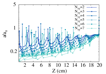
(a)

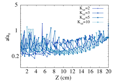
(b)

Figure 5: Plot of the fibre thickness $a/a_{0}$ as a function of the height from the the collecting plane at $Z=0$. We considered both asymmetric planar noises ($X/Y$ noise ratio $N_{sy}>1$) and vertical noises along the $Z$-axis ($XY/Z$ relative noise amplitude $N_{sz}=1$ and relative frequency $K_{sz}>1$). Parameters used for the simulations are $V_{0}=\;10^{4}$ V, $I_{F}=5\;10^{4}$, $N_{s}=10^{-3}$, $h=20$ cm. As for the 1D noise scenario the elongation profile strongly fluctuates with the height from the collecting plate, making asymmetric or vertical driving forces not desirable for optimal experimental set up.

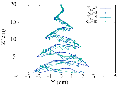
(a)

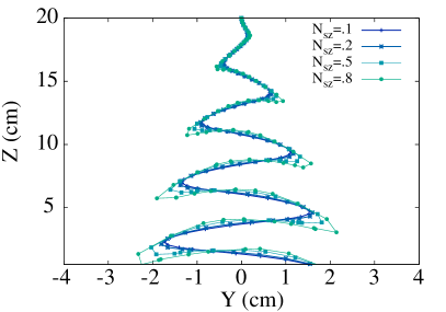
(b)

Figure 6: Spiral jet generated under the presence of a vertical driving force along the $Z$-axis on the pendant drop with a symmetric planar noise ($N_{sy}=1$). For clarity we plotted only the projection on the $ZY$-plane, but it should be noted that the spirals all keep they circular symmetry on the $XY$-plane. The parameters used for the simulations are $V_{0}=\;10^{4}$V, $I_{F}=5\;10^{4}$, $h=20$ cm. (a) Spiral structures for different values of the relative load frequency $K_{sz}$ to the planar noise frequency $K_{s}=5\;10^{3}$, and a fixed noise strength $N_{sz}=N_{s}=10^{-3}$. (b) Jet profile plotted for a range of relative noise intensities $N_{sz}$ with respect to the $XY$-plane noise $N_{s}=10^{-3}$ at a fixed frequency $K_{s}=5\;10^{3}$. The results indicate that even large vertical noises do not affect considerably the shape of the helix and in particular they do not lead to thinner fibres.

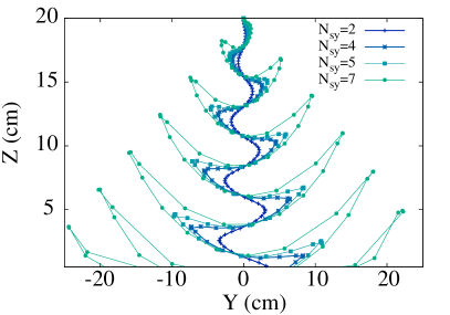
(a)

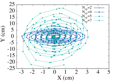
(b)

Figure 7: Plot of the jet profile projected on the $YZ$-plane (a) and $XY$-plane (b) for various relative intensities $N_{sy}$ of the noise along the $Y$-axis with respect to the noise $N_{s}$ on the $XY$-plane. $V_{0}=\;10^{4}$ V, $I_{F}=5\;10^{4}$, $N_{s}=10^{-3}$, $h=20$ cm. The greater the asymmetry in the noise, the larger the asymmetry in the helix profile as visible in (b). Note the scales of X and Y axes are significantly different here. This transition is rather fast to the point that above an asymmetry ratio of $N_{sy}=7$ we could not get stable numerical solutions any more, and already at $N_{sy}=7$ the helix gets deformed towards 1D banana shape profiles (Fig. 5(a)).

We also investigated the effect of planar noise asymmetry and vertical driving force with a range of frequencies (see Figs. 5-7). A wide variety of beautiful helices is obtained in this way, confirming the richness of the phenomenology shown by the dynamics of electrified jets. We found that the planar driving force remains the best design principle. In fact, by introducing asymmetry in the planar noise we quickly move towards the one-dimensional scenario with sharper turns that locally thicken the fibre. We also found that an additional vertical driving force does not provide a significant reduction of the fibre thickness. In the future we plan to include an additional component of the driving force along the $Z$-axis and/or consider an oscillating external field in the model.

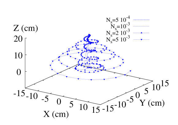
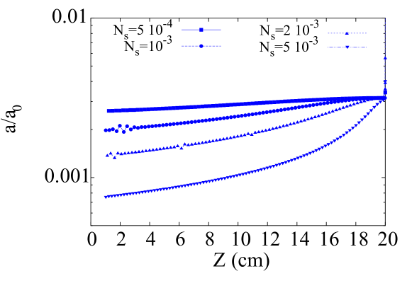
Figure 3: Effect on the spiral shape of the mechanical perturbation applied to the pendant drop. (a) Final configuration. Parameters used for the simulations are as above except for $N_{s}$. The plot shows the comparison of the profiles obtained with different values of the perturbation strength $N_{s}$. (b) Plot of the elongation along the spiral as a function of the distance from the collector. The plot shows a monotonic decrease of the fibre thickness as a function of the distance from the pendant drop. Finally, the plot highlights that an increase in the spiral radius induces an increase in the elongation of the electrified jet and correspondingly a reduction of the diameter of the resulting fibres.

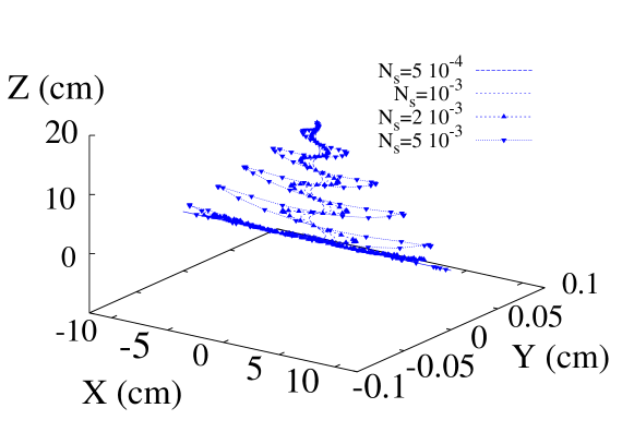
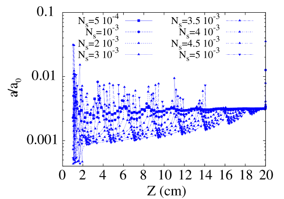
Figure 4: Effect on the spiral shape of the perturbation applied to the pendant drop only along the $X$-axis. a) Final configuration of the filament. Parameters used for the simulations are $V_{0}=\;10^{4}$ V, $\Omega=5\;10^{5}\;\text{s}^{-1}$ and $h=20$ cm. The plot compares the profiles obtained with different values of the noise strength $N_{s}$, with the jet oscillating only in the $XZ$-plane. (b) Plot of the elongation as a function of the distance from the collector. The spikes, not present in the case of the circular applied perturbation, correspond to the bending points that occur along the $Z$-axis.

IV.2 Effect of the perturbation frequency

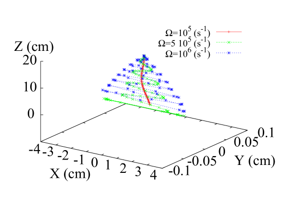
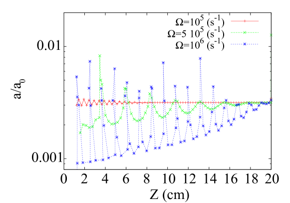
Figure 8: (a) The spiral structures for different values of the load frequency in the one-dimensional driving scenario along the $X$-axis. Parameters used for the simulations are $V_{0}=10^{4}$ V, $I_{F}=5\;10^{4}$, $N_{s}=10^{-3}$, $h=20$ cm. (b) Corresponding fibre extension plot, where the characteristic spikes due to the local bending are visible. As for the circular case, also in this case the increase in frequency results in thinner fibres.

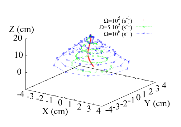
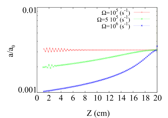
Figure 9: Comparison of the profiles obtained with different values of the perturbation frequency $\Omega$. Parameters used for the simulations are as above except for $\Omega$. (a) Final configuration of the filament under a circular perturbation. (b) Plot of the elongation as a function of the distance from the collector. Similarly to what observed by varying the perturbation strength (Fig. 3) also upon increasing the frequency $\Omega$ the radius of the spirals increases and stretches the fibre.

We have also explored the effect of the perturbation frequency, $\Omega$, by running a series of simulations with $\Omega=10^{4},10^{5},5\;10^{5},10^{6}\;\text{s}^{-1}$, for both planar and three-dimensional scenarios. The corresponding spiral structures are shown in Fig. 8 and in Fig. 9, respectively. From these figures, it is apparent that the main effect of increasing the perturbation frequency is to produce more compact and broader structures, i.e. spirals with a larger aperture and a shorter pitch. This can be traced back to the fact that, by increasing the perturbation frequency, the Coulomb repulsion in the $XY$-plane is enhanced, thus leading to larger ratio between the horizontal and vertical speeds, and hence a shorter pitch. Thus, increasing the frequency leads again to thinner fibres at the collector, offering an additional design parameter, which minimizes the fibre thickness. To the best of our knowledge, such a design parameter has not been considered before.

IV.3 Effect of the location of the perturbation source

In most experiments the polymer jet is seen to fall down along a straight-line configuration, prior to the development of bending instabilities. In other words, a vertical neck precedes the formation of spiral structures. Here, we have not been able to find any parameter regime for which the neck would smoothly develop into a spiral structure: the two configurations do not appear to belong together. What we have found instead is that spirals start precisely at the location where the perturbation is applied, which means that when the perturbation is applied at the spinneret, no neck is observed.

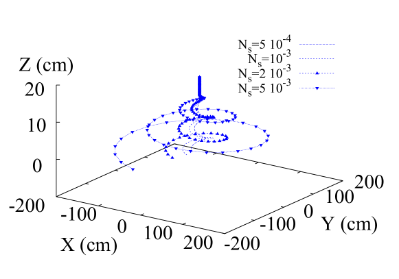
(a)

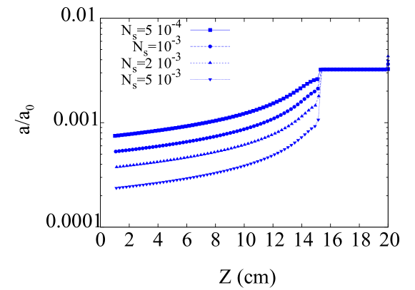
(b)

Figure 10: Effect on the spiral shape of the mechanical load applied $5$ cm below the pendant drop for various values of the load strength $N_{s}$. (a) Final configurations of the filament. Parameters are as above except for $N_{s}$. (b) Elongation as a function of the distance from the collector. Above the height of 15 cm, the location of the perturbation source, the fibre does not stretch appreciably.

To illustrate this point, in Fig. 10 we report the configuration of the spiral and the thickness of the jet, for a case where the perturbation is applied $5$ cm below the pendant drop. The jet shows a clear neck, up precisely to the point where the planar perturbation is applied. Subsequently, the spiral forms in the very same way as it did when the perturbation was placed at the pendant drop. A series of simulations was carried out by changing the location of the perturbation, always to find the same result: the spiral starts to develop precisely at the perturbation location. Furthermore, we have observed that, upon impinging on the collector, the jet forms planar coil patterns, similar to those observed in experiments, as one would expect for a thread falling on a stationary surface Chiu-Webster and Lister (2006).

These findings suggest that the presence of the neck might reflect a different and more elaborate pathway to instability than just mechanical perturbation at the spinneret. Among others, a possibility is provided by environmental fluctuations, say electrostatic or perhaps hydrodynamic ones, which may require a finite waiting time before building up sufficient strength to trigger bending instabilities. The importance of the formation of the neck on the development of the instability has been discussed in the work of Li et al. Li et al. (2013, 2006) where a detailed analysis of the initial step of the spinning process was developed and linked to the physico-chemical properties of the polymer solution jet. The results presented in the work of Li et al. suggest a strong dependence of the instability on such parameters. In the present study, we have also considered a broad spectrum of different physical parameters with respect to the one that define the nondimensional quantities in Table LABEL:tab:Real_Values (results not shown). For some values of the parameters we could not produce helices, suggesting that the properties of the polymer solutions strongly affect the instability process, hence in qualitative agreement with the results of Li et al. Li et al. (2013, 2006). However, even when we did detect helices, we still could not observe any qualitative change of the picture presented in this work, namely that planar oscillations driving the spinneret offer a viable route to produce much thinner fibres, regardless of the chemical physical properties of the polymer solution. A detailed analysis of the effect of the solutions used in the experiments will make the object of future work.

V Conclusions

Summarizing, we have presented a computational study of the effects of a fast-oscillating perturbation on the formation and dynamics of spiral structures in electrified jets used for electrospinning experiments. In particular, we have provided numerical evidence of a direct dependence of the spiral aperture on the perturbation amplitude and frequency. As a result, our simulations suggest that both parameters could be tuned in order to minimize the fibre thickness at the collector, by maximizing the spiral length. This might open up optimal design protocols in electrospinning experiments. In other words, independently of the rheology of the polymer solution, provided that fibres can be electrospun, applying a driving perturbation oscillating at high frequency at the pendant drop can further reduce the thickness.

V.1 Acknowledgements

M. Bernaschi and U. Amato are kindly acknowledged for computational help with the project. The research leading to these results has received funding from the European Research Council under the European Union’s Seventh Framework Programme (FP/2007-2013)/ERC Grant Agreement n. 306357 (ERC Starting Grant “NANO-JETS”). One of the authors (SS) wishes to acknowledge the Erwin Schroedinger Institute (ESI), for kind hospitality and financial support under the ESI Senior Fellow program.

References

- Yarin (1993) Alexander L Yarin, Free liquid jets and films: Hydrodynamics and rheology (Longman Scientific & Technical (New York), 1993).
- Reneker et al. (2000) Darrell H. Reneker, Alexander L. Yarin, Hao Fong, and Sureeporn Koombhongse, “Bending instability of electrically charged liquid jets of polymer solutions in electrospinning,” Journal of Applied Physics 87, 4531 (2000).
- Yarin et al. (2001) A. L. Yarin, S. Koombhongse, and D. H. Reneker, “Taylor cone and jetting from liquid droplets in electrospinning of nanofibers,” Journal of Applied Physics 90, 4836 (2001).
- Loscertales et al. (2002) I G Loscertales, A Barrero, I Guerrero, R Cortijo, M Marquez, and A M Gañán Calvo, “Micro/nano encapsulation via electrified coaxial liquid jets.” Science (New York, N.Y.) 295, 1695–8 (2002).
- Dzenis (2004) Yuris A Dzenis, “Spinning Continuous Fibers for Nanotechnology Spinning Continuous Fibers for Nanotechnology,” Science 304, 1917–1919 (2004).
- Helgeson et al. (2008) Matthew E. Helgeson, Kristie N. Grammatikos, Joseph M. Deitzel, and Norman J. Wagner, “Theory and kinematic measurements of the mechanics of stable electrospun polymer jets,” Polymer 49, 2924–2936 (2008).
- Thompson et al. (2007) C. J. Thompson, G. G. Chase, A. L. Yarin, and D.H. Reneker, “Effects of parameters on nanofiber diameter determined from electrospinning model,” Polymer 48, 6913–6922 (2007).
- Grafahrend et al. (2011) Dirk Grafahrend, Karl-Heinz Heffels, Meike V Beer, Peter Gasteier, Martin Möller, Gabriele Boehm, Paul D Dalton, and Jürgen Groll, “Degradable polyester scaffolds with controlled surface chemistry combining minimal protein adsorption with specific bioactivation.” Nature materials 10, 67–73 (2011).
- Greenfeld et al. (2012) Israel Greenfeld, Kamel Fezzaa, Miriam H. Rafailovich, and Eyal Zussman, “Fast X-ray Phase-Contrast Imaging of Electrospinning Polymer Jets: Measurements of Radius, Velocity, and Concentration,” Macromolecules 45, 3616–3626 (2012).
- Onses et al. (2013) M. Serdar Onses, Chiho Song, Lance Williamson, Erick Sutanto, Placid M. Ferreira, Andrew G. Alleyne, Paul F. Nealey, Heejoon Ahn, and John A. Rogers, “Hierarchical patterns of three-dimensional block-copolymer films formed by electrohydrodynamic jet printing and self-assembly.” Nature nanotechnology 8, 667–75 (2013).
- Min et al. (2013) Sung-Yong Min, Tae-Sik Kim, Beom Joon Kim, Himchan Cho, Yong-Young Noh, Hoichang Yang, Jeong Ho Cho, and Tae-Woo Lee, “Large-scale organic nanowire lithography and electronics.” Nature communications 4, 1773 (2013).
- Regev et al. (2013) Omri Regev, Arkadii Arinstein, and Eyal Zussman, “Creep anomaly in electrospun fibers made of globular proteins,” Physical Review E 88, 062605 (2013).
- Nakano et al. (2012) Atsushi Nakano, Norihisa Miki, Koichi Hishida, and Atsushi Hotta, “Solution parameters for the fabrication of thinner silicone fibers by electrospinning,” Physical Review E 86, 011801 (2012).
- Greiner and Wendorff (2007) Andreas Greiner and Joachim H Wendorff, “Electrospinning: a fascinating method for the preparation of ultrathin fibers.” Angewandte Chemie (International ed. in English) 46, 5670–703 (2007).
- Fridrikh et al. (2003) Sergey Fridrikh, Jian Yu, Michael Brenner, and Gregory Rutledge, “Controlling the Fiber Diameter during Electrospinning,” Physical Review Letters 90, 144502 (2003).
- Camposeo et al. (2013) Andrea Camposeo, Luana Persano, and Dario Pisignano, “Light-Emitting Electrospun Nanofibers for Nanophotonics and Optoelectronics,” Macromolecular Materials and Engineering 298, 487–503 (2013).
- Pisignano (2013) Dario Pisignano, Polymer Nanofibers: Building Blocks for Nanotechnology, 29 (Royal Society of Chemistry, 2013).
- Taylor (1969) G. Taylor, “Electrically Driven Jets,” Proceedings of the Royal Society A: Mathematical, Physical and Engineering Sciences 313, 453–475 (1969).
- Marin et al. (2008) Alvaro G. Marin, Guillaume Riboux, Ignacio G Loscertales, and Antonio Barrero, “Whipping Instabilities in Electrified Liquid Jets,” , 3 (2008), arXiv:0810.0155 .
- Liu et al. (2005) Haiqing Liu, Christian H. Reccius, and H. G. Craighead, “Single electrospun regioregular poly(3-hexylthiophene) nanofiber field-effect transistor,” Applied Physics Letters 87, 253106 (2005).
- Persano et al. (2014) Luana Persano, Andrea Camposeo, Pompilio Del Carro, Vito Fasano, Maria Moffa, Rita Manco, Stefania D’Agostino, and Dario Pisignano, “Lasers: Distributed Feedback Imprinted Electrospun Fiber Lasers,” Advanced Materials 26, 6542–6547 (2014).
- Moran-Mirabal et al. (2007) José M Moran-Mirabal, Jason D Slinker, John a DeFranco, Scott S Verbridge, Rob Ilic, Samuel Flores-Torres, Héctor Abruña, George G Malliaras, and H G Craighead, “Electrospun light-emitting nanofibers.” Nano letters 7, 458–63 (2007).
- Vohra et al. (2011) Varun Vohra, Umberto Giovanella, Riccardo Tubino, Hideyuki Murata, and Chiara Botta, “Electroluminescence from conjugated polymer electrospun nanofibers in solution processable organic light-emitting diodes.” ACS nano 5, 5572–8 (2011).
- Kakade et al. (2007) Meghana V Kakade, Steven Givens, Kenncorwin Gardner, Keun Hyung Lee, D Bruce Chase, and John F Rabolt, “Electric field induced orientation of polymer chains in macroscopically aligned electrospun polymer nanofibers.” Journal of the American Chemical Society 129, 2777–82 (2007).
- Pagliara et al. (2011) Stefano Pagliara, Miriam S. Vitiello, Andrea Camposeo, Alessandro Polini, Roberto Cingolani, Gaetano Scamarcio, and Dario Pisignano, “Optical Anisotropy in Single Light-Emitting Polymer Nanofibers,” The Journal of Physical Chemistry C 115, 20399–20405 (2011).
- Richard-Lacroix and Pellerin (2012) Marie Richard-Lacroix and Christian Pellerin, “Orientation and Structure of Single Electrospun Nanofibers of Poly(ethylene terephthalate) by Confocal Raman Spectroscopy,” Macromolecules 45, 1946–1953 (2012).
- Pagliara et al. (2009) Stefano Pagliara, Andrea Camposeo, Alessandro Polini, Roberto Cingolani, and Dario Pisignano, “Electrospun light-emitting nanofibers as excitation source in microfluidic devices.” Lab on a chip 9, 2851–6 (2009).
- Xie et al. (2009) Jingwei Xie, Matthew R MacEwan, Xiaoran Li, Shelly E Sakiyama-Elbert, and Younan Xia, “Neurite outgrowth on nanofiber scaffolds with different orders, structures, and surface properties.” ACS nano 3, 1151–9 (2009).
- Arinstein et al. (2007) Arkadii Arinstein, Michael Burman, Oleg Gendelman, and Eyal Zussman, “Effect of supramolecular structure on polymer nanofibre elasticity.” Nature nanotechnology 2, 59–62 (2007).
- Hohman et al. (2001a) Moses M. Hohman, Michael Shin, Gregory Rutledge, and Michael P. Brenner, “Electrospinning and electrically forced jets. I. Stability theory,” Physics of Fluids 13, 2201 (2001a).
- Hohman et al. (2001b) Moses M. Hohman, Michael Shin, Gregory Rutledge, and Michael P. Brenner, “Electrospinning and electrically forced jets. II. Applications,” Physics of Fluids 13, 2221 (2001b).
- Greenfeld et al. (2011) Israel Greenfeld, Arkadii Arinstein, Kamel Fezzaa, Miriam H. Rafailovich, and Eyal Zussman, “Polymer dynamics in semidilute solution during electrospinning: A simple model and experimental observations,” Physical Review E 84, 041806 (2011).
- Pontrelli et al. (2014) Giuseppe Pontrelli, Daniele Gentili, Ivan Coluzza, Dario Pisignano, and Sauro Succi, “Effects of non-linear rheology on electrospinning process: A model study,” Mechanics Research Communications 61, 41–46 (2014), arXiv:1405.6075 .
- Sun et al. (2006) Daoheng Sun, Chieh Chang, Sha Li, and Liwei Lin, “Near-field electrospinning.” Nano letters 6, 839–42 (2006).
- Bisht et al. (2011) Gobind S Bisht, Giulia Canton, Alireza Mirsepassi, Lawrence Kulinsky, Seajin Oh, Derek Dunn-Rankin, and Marc J Madou, “Controlled continuous patterning of polymeric nanofibers on three-dimensional substrates using low-voltage near-field electrospinning.” Nano letters 11, 1831–7 (2011).
- Pai et al. (2011) Chia-Ling Pai, Mary C. Boyce, and Gregory C. Rutledge, “Mechanical properties of individual electrospun PA 6(3)T fibers and their variation with fiber diameter,” Polymer 52, 2295–2301 (2011).
- Yarin (1990) Alexander L. Yarin, “Strong flows of polymeric liquids,” Journal of Non-Newtonian Fluid Mechanics 37, 113–138 (1990).
- Reneker and Yarin (2008) Darrell H. Reneker and Alexander L. Yarin, “Electrospinning jets and polymer nanofibers,” Polymer 49, 2387–2425 (2008).
- Bhattacharjee and Rutledge (2011) P. K. Bhattacharjee and G. C. Rutledge, Comprehensive Biomaterials, edited by P. Ducheyne, K. E. Healy, D. W. Hutmacher, D. W. Grainger, and C. J. Kirkpatrick (Elsevier, Oxford, 2011).
- Chiu-Webster and Lister (2006) S. Chiu-Webster and J. R. Lister, “The fall of a viscous thread onto a moving surface: a ‘fluid-mechanical sewing machine’,” Journal of Fluid Mechanics 569, 89 (2006).
- Li et al. (2013) Fang Li, Alfonso M. Gañán Calvo, José M. López-Herrera, Xie-Yuan Yin, and Xie-Zhen Yin, “Absolute and convective instability of a charged viscoelastic liquid jet,” Journal of Non-Newtonian Fluid Mechanics 196, 58–69 (2013).
- Li et al. (2006) Fang Li, Xie-Yuan Yin, and Xie-Zhen Yin, “Instability analysis of a coaxial jet under a radial electric field in the nonequipotential case,” Physics of Fluids 18, 037101 (2006).