The impact of cosmic variance on simulating weak lensing surveys

Abstract

Upcoming weak lensing surveys will survey large cosmological volumes to measure the growth of cosmological structure with time and thereby constrain dark energy. One major systematic uncertainty in this process is the calibration of the weak lensing shape distortions, or shears. Most upcoming surveys plan to test several aspects of their shear estimation algorithms using sophisticated image simulations that include realistic galaxy populations based on high-resolution data from the Hubble Space Telescope (HST). However, existing datasets from the HST cover very small cosmological volumes, so cosmic variance could cause the galaxy populations in them to be atypical. A narrow redshift slice from such surveys could be dominated by a single large overdensity or underdensity. In that case, the morphology-density relation could alter the local galaxy populations and yield an incorrect calibration of shear estimates as a function of redshift. We directly test this scenario using the COSMOS survey, the largest-area HST survey to date, and show how the statistical distributions of galaxy shapes and morphological parameters (e.g., Sérsic $n$) are influenced by redshift-dependent cosmic variance. The typical variation in RMS ellipticity due to environmental effects is 5 per cent (absolute, not relative) for redshift bins of width $\Delta z=0.05$, which could result in uncertain shear calibration at the 1 per cent level. We conclude that the cosmic variance effects are large enough to exceed the systematic error budget of future surveys, but can be mitigated with careful choice of training dataset and sufficiently large redshift binning.

1 Introduction

Weak gravitational lensing, the deflection of light by mass, is one of the cleanest ways to study the nature of dark energy by tracking the growth of structure in the Universe as a function of time (e.g., Bartelmann & Schneider, 2001; Albrecht et al., 2006; Weinberg et al., 2013). As light from background sources passes by matter (including dark matter) on its way to us, the apparent shapes of the background galaxies get distorted, and the galaxies get slightly magnified as well. Because of its sensitivity to dark matter and dark energy, major surveys such as the Hyper Suprime-Cam (HSC; Miyazaki et al., 2006), Dark Energy Survey (DES; The Dark Energy Survey Collaboration, 2005), the KIlo-Degree Survey (KIDS; de Jong et al., 2013), the Panoramic Survey Telescope and Rapid Response System (PanSTARRS; Kaiser et al., 2010), the Large Synoptic Survey Telescope (LSST; LSST Science Collaboration et al., 2009), Euclid (Laureijs et al., 2011), and Wide-Field Infrared Survey Telescope (WFIRST; Green et al., 2012) are planned for the next two decades to gather enormous quantities of weak lensing data that will lead to precise constraints on the growth of structure with time, and therefore cosmological parameters.

For the upcoming surveys to achieve their promise, their systematic error budgets must be below their statistical error budgets. Systematic error budgets for weak lensing surveys typically include astrophysical effects, such as intrinsic alignments of galaxy shapes with large scale density fields (e.g., Troxel & Ishak, 2014) and the effect of baryons on the matter power spectrum (e.g., van Daalen et al., 2011; Semboloni et al., 2011), as well as observational uncertainties such as the ability to robustly infer shears from observed galaxy shapes or photometric redshifts from their observed colours. Given the expected sub-per cent statistical errors on upcoming surveys, systematic errors must be reduced from their typical level in the current state-of-the-art measurements that typically achieve $\sim 5$ per cent statistical errors at best (e.g., Schrabback et al., 2010; Heymans et al., 2013; Jee et al., 2013; Mandelbaum et al., 2013).

Some types of information about and tests of shear estimation for ongoing and future weak lensing surveys will rely on data from the Hubble Space Telescope (HST). For example, data from HST can be used to derive basic statistics of galaxy light profiles, such as joint distributions of size and the morphology. It can be used to infer the intrinsic distribution of galaxy shapes, which enters the shear estimation process either implicitly or explicitly depending on the method used for shear estimation (see, e.g., Viola, Kitching & Joachimi, 2014). Going beyond basic information about the light profile, HST can be used to quantify the detailed morphology of galaxies, due to its higher resolution compared to any current or planned weak lensing survey. Finally, it can be used to address systematics due to colour gradients within galaxies, which are particularly problematic when combined with a wavelength-dependent diffraction-limited PSF (e.g., Voigt et al., 2012; Semboloni et al., 2013).

One method that is commonly used to test for the presence of systematic errors in the shear estimation process is image simulation, where we can cleanly test whether our methods of shear estimation recover the ground truth. This is a valuable test, considering the numerous sources of additive and multiplicative bias such as a mismatch between galaxy model assumptions and actual galaxy light profiles (e.g., Voigt & Bridle, 2010; Melchior et al., 2010), biases due to the effects of pixel noise on the shear estimates (Kacprzak et al., 2012; Melchior & Viola, 2012; Refregier et al., 2012), and ellipticity gradients (Bernstein, 2010). These biases often differ for galaxies with different morphologies (e.g., disks vs. ellipticals), sizes, $S/N$, and shape (Bridle et al., 2010; Kitching et al., 2012). A general requirement for simulations used to test shear recovery is that they should be as realistic as possible.

Realistic simulations may use samples based on images from the (HST). Software packages like GalSim (Rowe et al., 2014) can generate images of galaxies from the HST as they would appear with an additional lensing shear and viewed by some lower resolution telescope. Examples of training samples from the HST include the COSMOS survey (used by the GREAT3 challenge, Mandelbaum et al., 2014) or the Ultra Deep Field (UDF, used by Jee et al., 2013). These two examples serve as the extremes in the HST samples used as the basis for image simulation, with COSMOS being the widest contiguous area surveyed by the HST currently and hence representive, and the latter being extremely deep but narrow.

For a variety of physical reasons, some of which are still not fully understood, the shape and morphology of galaxies depends on their local environment (e.g., Carollo et al., 2014; De Propris et al., 2014). Hence, local overdensities or underdensities along the line of sight observed in these HST fields may (given the small size of the field) cause the properties of the galaxy population in redshift slices to be atypical depending on the environment in that slice. This has the undesired consequence of including a variation in galaxy properties due to the COSMOS (or other) survey cosmic variance in the simulated galaxy sample in that redshift slice, rather than only including ensemble effects that would appear in a large cosmological volume, such as true redshift evolution of galaxy properties. Our goal is to quantify the degree to which the morphology-density correlations in COSMOS cause noticeable changes in the galaxy populations in narrow redshift slices at a level that could result in difficulty using the sample to derive redshift-dependent shear calibrations. Upcoming surveys will study lensing as a function of redshift and therefore need to simulate galaxy samples at different redshifts in order to assess the shear calibration at each redshift.

The paper is structured as follows: in Sec. 2, we describe the data that we use for this study. In Sec. 3, we describe our methods for deriving the relevant galaxy properties like environment, morphology, and shape. Using these ingredients, we present our results in Sec. 4 and discuss their implications in Sec. 5, concluding in Sec. 6.

2 Data

The COSMOS survey (Scoville et al., 2007; Koekemoer et al., 2007; Leauthaud et al., 2007) is a flux-limited, narrow deep field survey covering a contiguous area of $1.64\text{ deg}^{2}$ of sky, with images taken using the Advanced Camera for Surveys (ACS) Wide Field Channel (WFC) in the Hubble Space Telescope (HST). We use the COSMOS survey to define a parent sample of galaxy images to be used for making image simulations, following the approach taken in Mandelbaum et al. (2012, 2014).

We apply the following set of initial cuts to the COSMOS data, the first two of which are motivated and explained in more detail by Leauthaud et al. (2007):

1. MU_CLASS=1: This criterion uses a comparison between the peak surface brightness and the background level to achieve a robust star/galaxy separation, with galaxies having MU_CLASS=1.

2. CLEAN=1: Objects near bright stars or those containing saturated pixels were removed; the rest pass this cut on CLEAN.

3. GOOD_ZPHOT_SOURCE =1: This cut requires that photometric redshifts be reliable and good enough to draw conclusions about the population (see Mandelbaum et al. 2012 for details).

High resolution images taken through the wide F814W filter (broad I) for all galaxies passing the above cuts were used to create a collection of postage stamp images for the GREAT3 challenge (Mandelbaum et al., 2014), using the procedure described in Mandelbaum et al. (2012). Each galaxy postage stamp image has a corresponding PSF image that can be used by GalSim or other software to remove the effects of the HST PSF before simulating the galaxy image as it would appear at lower resolution.

To better characterize the galaxy population, parametric models were fit to the light profiles of these galaxies. These were carried out using the method described in Lackner & Gunn (2012), and include Sérsic profile fits and 2 component bulge $+$ disk fits described in detail in Mandelbaum et al. (2014) and briefly in Sec. 3.3 of this work.

In addition to the ACS/WFC (F814W) imaging, the COSMOS field has also been imaged by Subaru Suprime-Cam, the Canada-French Hawaii Telescope (CFHT) and KPNO/CTIO, yielding many bands of imaging data used to determine high-fidelity photometric redshifts. Photometric redshifts were determined by Ilbert et al. (2009). The accuracy of photometric redshifts for $m_{\text{F814W}}\leq$ 22.5 is $\sigma_{\Delta z}=0.007(1+z)$; for $m_{\text{F814W}}\leq$ 24, $\sigma_{\Delta z}=0.012(1+z)$. The photometric redshift values become noisier beyond $z\sim 1.2$, and the fits to the galaxy light profiles are also somewhat noisy once we go beyond $m_{\text{F814W}}\sim 23.5$. For this reason, we will exclude all galaxies that have F814W magnitude fainter than 23.5. However, we will use the $m_{\text{F814W}}\leq 25.2$ sample that was generated for the GREAT3 challenge to estimate the completeness, which is useful when generating a volume-limited sample (Sec. 3.2). We first use the $z\leq 1.25$ flux-limited sample to fit parametric redshift distribution models (Sec. 3.1), and then restrict ourselves to $z\leq 1$ sample for all further analysis.

Stellar mass estimates were obtained (Leauthaud et al., 2010) using the Bayesian code described in Bundy et al. (2006). This process involves constructing a grid of models that vary in age, star formation history, dust content and metallicity (always assuming a Chabrier IMF; Chabrier 2003), to which the observed galaxy spectral energy distributions (SEDs) and photometric redshift are compared. At each grid point, the probability that the SED fits the model is calculated, and by marginalizing over the nuisance parameters in the grid, the stellar mass probability distribution is obtained. The median of this distribution is taken as the stellar mass estimate.

3 Methods

In order to study the variation in the intrinsic ellipticity distribution and various morphological indicators with the galaxy environment, there are three main steps to be carried out:

1. Identify overdense and underdense environments along the line of sight in our survey from the redshift distribution of galaxies (Sec. 3.1);

2. volume-limit the sample such that Malmquist bias is minimized before comparing galaxies in different redshift slices (Sec. 3.2); and

3. estimate the galaxy axis ratios and other morphological indicators such as Sérsic index and bulge-to-total ratios (Sec. 3.3).

In this section we will describe how these steps were carried out.

3.1 Finding overdensities

Figure 1: Upper panel: Redshift distribution of flux-limited ($m_{\text{F814W}}\leq 23.5$) sample with photometric redshift bins that are 0.05 wide. The vertical line at $z=0.3$ indicates the delineation between lower redshifts that we do not use for our analysis, and higher redshifts that are used. Fits to two analytical functions, $p_{1}(z)$ and $p_{2}(z)$, defined in Eqs. 1 and 2, are also shown, with best-fitting parameters $a=2.53\pm 0.98$, $z_{1}=0.32\pm 0.16$, $b=1.70\pm 0.50$ and $z_{2}=0.63\pm 0.13$. We also show the distributions from Coil et al. (2004) from Eqs. 3 and 4. Lower panel: Plot of $\delta_{g,\text{1D}}=N/N_{\text{mod}}-1$ with each functional form as the model for each redshift bin.

It is important to keep in mind when considering the environment estimation that our goal is not to create a full 3D mapping of the density field within the COSMOS region (a task that was already addressed by Kovač et al. 2010 using the zCOSMOS spectroscopic sample). Instead, we make a coarse, 1-dimensional, line of sight division of the COSMOS survey into redshift slices, just as would be done when making galaxy redshift slices as input to a weak lensing survey simulation. For each redshift slice, we can then check whether the environment is overdense or underdense on average. Our approach will tend to wash out some real trends from a 3D study, but is appropriate given our scientific goal of testing effects of the environment on weak lensing simulations based on the COSMOS survey.

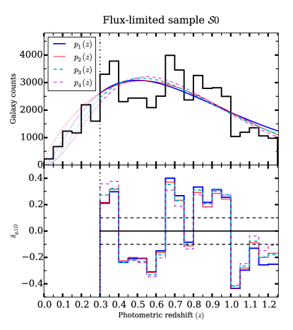
For our (flux-limited) sample of galaxies, up to $z=1.25$, we fit parametric models to the histograms of photometric redshifts in order to assign values of overdensity. We choose our bins to be $0.05$ wide starting from $z=0.3$, where the bin width is selected to be somewhat larger than the photometric redshift error but narrow enough that we can still identify rather than averaging over real cosmological structures. We neglect the lowest redshifts which have negligible cosmological volume and where the galaxy population tends to be intrinsically bright and large enough that a non-negligible fraction is lost due to the cuts we impose (Sec. 2).

The parametric redshift distributions that we use are

$$p_{1}(z)\propto z^{a-1}\exp\left[{-z/z_{1}}\right]$$ (1)

and

$$p_{2}(z)\propto z^{b-1}\exp\left[-\frac{1}{2}\left(\frac{z}{z_{2}}\right)^{2}\right]$$ (2)

Here $a$, $b$, $z_{1}$ and $z_{2}$ are free parameters that are to be determined. The normalization constants depend not only on the parameters but also on the lower and the upper limit of the redshifts considered, where we fix the normalization to ensure that the predicted number of galaxies in the range used ($0.3<z<1.25$) is equal to the actual number. Fig. 1 shows the photometric redshift histogram together with the best-fitting parametric distributions.

We compare our fits to the fits made by Coil et al. (2004) using the DEEP2 galaxy redshift survey. Interpolating between their results for the $18<I_{\text{AB}}<23$ and $18<I_{\text{AB}}<24$ samples to our own limiting magnitude (and assuming equivalence of our $I$ bands), we obtain the following redshift distributions:

$$p_{3}(z)\propto z^{2}\exp{[-z/0.262]}$$ (3)

and

$$p_{4}(z)\propto z^{2}\exp{[-(z/0.361)^{1.2}]}$$ (4)

which are also plotted in Fig. 1. Note that $p_{3}(z)$ is a special case of $p_{1}(z)$ with $a=3$ and $z_{1}=0.262$; these parameter values are within the $1\sigma$ allowed regions for our fits to Eq. 1. Visually, these distributions appear quite similar to our own fits carried out here, which is reassuring given the use of different survey data and functional forms.

The estimated overdensity in a redshift bin is defined by comparing the observed galaxy counts in the bin with the counts that are predicted in that bin by one of the models in Eqs. (1) and (2):

$$\delta_{g,\text{1D}}=\frac{(N-N_{\text{mod}})}{N_{\text{mod}}},$$ (5)

where

$$N_{\text{mod}}=\int_{z_{\text{min}}}^{z_{\text{max}}}p(z)\,\mathrm{d}z$$ (6)

is determined by integrating the redshift distribution within the limits of that redshift slice. Note that $\delta_{g,\text{1D}}$ is dependent on our choice of model redshift distribution, and should have a mean value of $0$ over the entire redshift range when weighted by the number fraction in each bin.

Our preliminary decision criterion for identifying overdense and underdense redshift slices involves leaving a 10 per cent margin around an overdensity of zero; i.e., if $\left|\delta_{g,\text{1D}}\right|<0.1$, that is considered “neutral” (neither overdense nor underdense on average). We can then label each redshift slice as either overdense, underdense, or neutral as follows: We label a redshift bin as overdense if at least one model gives a value of $\delta_{g,\text{1D}}>0.1$ while the other gives $\delta_{g,\text{1D}}>-0.1$ (neutral or overdense), and vice versa for the underdense regions. We label a redshift bin as neutral if both models give $\delta_{g,\text{1D}}$ within the neutral region, or if use of one model redshift distribution results in the conclusion that the bin is overdense while the other leads to the conclusion that it is underdense.

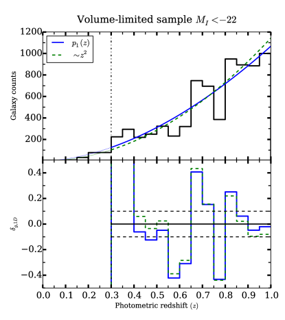
Once we volume-limit our sample (explained in Sec. 3.2), we again compare the histogram to the models. If there is no qualitative change in the overdensities, we stick with the preliminary decision. If the overdensity values flip in sign or become too small, then we classify the redshift bin as ‘neutral’. The naive Poisson uncertainty of the counts in each bin is much less than the difference between the actual number of galaxies present and the number predicted by the models. For this reason, errorbars have been completely ignored.

We thus identify the regions $z=0.30-0.40$, $0.65-0.75$, and $0.80-0.85$ as overdense; $z=0.55-0.65$ and $0.75-0.80$ as underdense; and we defer classication of the somewhat ambiguous range from $z=0.40-0.55$ until Sec. 3.2.

We have adopted this purely 1D environment classification for reasons explained at the beginning of this section. However, as a sanity check we can compare it with a more rigorous study that includes information about structure in the plane of the sky. Kovač et al. (2010) used a sample of $\sim$10 000 zCOSMOS spectroscopic galaxies with $I_{AB}<22.5$ to reconstruct the three dimensional overdensity field up to $z\sim 1$. We find that our classification of overdensities and underdensities agrees with this work, except for our two highest redshift bins. We believe that this disagreement is due to the errors in our photometric redshifts, with the overdensity reported by Kovač et al. (2010) in the $z=0.875-1$ range leaking into our $z=0.80-0.85$ slice.

Figure 2: Distribution of absolute magnitude $M_{I}$ for various flux-limited samples in the redshift range $[0.80,0.85]$ are plotted together. The vertical line corresponds to our luminosity cut of $-20.8$, brighter than which the $m_{\text{F814W}}<23.5$ sample includes $>95.3$ per cent of the galaxies in the $m_{\text{F814W}}<25.2$ sample.

3.2 Volume-limiting

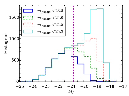
COSMOS is a flux-limited survey and is therefore affected by Malmquist bias, with the galaxy samples at higher redshifts being intrinsically brighter on average. Our analysis involves comparing galaxies in different redshift slices to identify significant differences in morphology that arise due to morphology-density correlations. Such an analysis would be very difficult with a flux-limited sample because there would be some variation in morphology with redshift just due to the intrinsic change in the sample properties. For a fair comparison, we must restrict ourselves to galaxies that are bright enough that they would be observed at all redshifts that we consider, which is achieved by volume-limiting the sample. We consider three different ways of carrying out this process, which results in three different galaxy sample selections, all of which we will use in the remainder of the analysis.

Call the flux-limited ($m_{\text{F814W}}\leq 23.5$) sample $\mathcal{S}$$0$. Our first approach is to generate a volume-limited sample that is complete up to $z=1$, by applying a cut on luminosity such that only galaxies instrinsically brighter than a certain threshold (determined in detail below) are considered. This threshold is set on the $k$-corrected $I$-band absolute magnitudes ($M_{I}$) from the COSMOS PSF-matched photometry catalog. Since the parent sample contains fainter galaxies and is quite complete to $m_{\text{F814W}}=25.2$, we compare the $M_{I}$ distribution of the $m_{\text{F814W}}=23.5$ sample with flux-limited samples that have fainter flux limits, to see where the $m_{\text{F814W}}<23.5$ sample that we want to use for our tests is no longer complete. At $M_{I}\sim-22.0$, the $m_{\text{F814W}}<23.5$ sample is beginning to lose galaxies in the $0.9<z<1.0$ redshift bin due to the flux limit. However, the $0.85<z<1$ redshift bin was found to be only moderately overdense, so we choose to disregard this region for the rest of the analysis, and instead restrict to $z<0.85$, which is advantageous because it allows us to choose a somewhat fainter intrinsic luminosity limit for the analysis. We relax our luminosity cut so that the sample is volume-limited not until $z=1$ but until $z=0.85$. We impose the cut at $M_{I}=-20.8$, which gives 95.3 per cent completeness in the $0.8<z\leq 0.85$ bin (see Fig. 2). The resulting sample, which has 13 567 galaxies, will be called sample $\mathcal{S}$$1$ in the remainder of this work.

However, previous studies (e.g., Wolf et al., 2003; Giallongo et al., 2005; Willmer et al., 2006; Faber et al., 2007) have shown that galaxy intrinsic luminosities evolve with redshift. Thus, we should also let the luminosity cut that we apply to volume-limit the sample evolve with redshift. Unfortunately, the majority of the published work on evolution of the luminosity function uses $B$ and $V$ band data, and it is not apparent that the results should be the same in a redder passband like $I$. We use the results from Faber et al. (2007) for the evolution of $B$-band magnitudes from the DEEP2 and COMBO-17 surveys, which is $\Delta M_{B}^{*}\sim-1.23$ mag per unit redshift (with the sign indicating that galaxies were intrinsically brighter in the past), for a combined sample of blue and red galaxies. Typically, estimates of evolution in the redder bands are less than the estimates of evolution in bluer bands (Lin et al., 1999; Blanton et al., 2003). Assuming that the evolution is a smooth function of the wavelength, the evolution in $I$-band should be in between $B$ and $K$ band. Therefore, by considering no evolution (a lower limit) as in our $\mathcal{S}$$1$, and a second sample $\mathcal{S}$$2$ constructed using the $B$-band evolution (as an upper bound on the $I$-band evolution), we can assume that these two samples bracket reality.

Thus, $\mathcal{S}$$2$ is constructed by letting the luminosity cut evolve, starting from $M_{I}=-20.8$ (same as in $\mathcal{S}$$1$) for the $0.8<z\leq 0.85$ bin. The cut values for the other bins are defined by allowing $1.23$ magnitudes of evolution to fainter magnitudes as a function of redshift (evaluated using the bin centers). Because of the sign of redshift evolution, $\mathcal{S}$$2$ includes more galaxies (15 903 galaxies).

One might wonder why we cannot use the luminosity function in F814W based on the COSMOS observations to directly determine the rate of evolution of the luminosity function for our sample, thus simplifying this exercise. However, this turns out to be highly non-trivial for two reasons. First, the F814W observations are relatively shallow compared to the deep ground-based observations used in many other works for determination of luminosity evolution. As a result, it is difficult to get a handle on the faint end of the luminosity function, and the unknown faint-end slope turns out to be degenerate with the evolution of the typical luminosity. Second, the photometric redshift error is a complicating factor that requires sophisticated techniques to remove. A derivation of the $I$-band luminosity evolution is therefore beyond the scope of this work.

Finally, we can circumvent the problem of redshift evolution of the luminosity by imposing cuts on stellar mass instead. In Fig. 3, we show the stellar mass function (SMF) of our sample for various F814W flux limits. The shapes of the SMF curves we obtain are consistent with those in Tomczak et al. (2014) at the high stellar-mass end. Tomczak et al. (2014) report the SMFs for the ZFOURGE survey, which includes COSMOS. They calculated stellar masses using the procedure and software described by Kriek et al. (2009), using a set of models with exponentially declining star formation history (Bruzual & Charlot, 2003) assuming a Chabrier IMF (Chabrier, 2003). As done for $M_{I}$, we compare the stellar mass function of the $m_{\text{F814W}}\leq 23.5$ sample with that of the $m_{\text{F814W}}\leq 25.2$ sample. The sample with $\log(M/M_{\odot})>10.15$ is $\sim 95$ per cent complete in the redshift bin $0.75\leq z<0.85$ and has 8953 galaxies in total across all redshifts. Thus, we construct a third volume-limited sample $\mathcal{S}$$3$ by imposing the stellar mass cut mentioned above.

The numbers of galaxies in redshift slices are tabulated in Table 1 for all three ways discussed in this section of obtaining a volume-limited sample. The stellar-mass limited sample is the smallest, most likely because when converting from flux to stellar mass, the stellar mass-to-light ratios vary strongly with galaxy type, so red galaxies with high $M_{*}/L$ simply have too low a flux compared to the blue galaxies at the same $M_{*}$, and are not observed.

Redshift	Environment	$\mathcal{S}$$1$	$\mathcal{S}$$2$	$\mathcal{S}$$3$
0.3-0.4	Overdense	1726	2505	1260
0.4-0.475	Neutral	988	1312	708
0.475-0.55	Neutral	1410	1793	904
0.55-0.65	Underdense	1797	2193	1183
0.65-0.7	Overdense	2096	2321	1354
0.7-0.75	Overdense	1963	2155	1239
0.75-0.8	Underdense	1159	1196	675
0.8-0.85	Overdense	2428	2428	1630

Table 1: List of different redshift bins, their environmental classification and the number of galaxies per redshift bin for volume-limited samples constructed in three different ways: using a hard luminosity cut ($\mathcal{S}$$1$), using a redshift-dependent luminosity cut ($\mathcal{S}$$2$) and using stellar-mass cuts ($\mathcal{S}$$3$).

Figure 3: Stellar mass distribution for various flux-limited samples are shown in three redshift ranges as separate panels. The redshift bins have been chosen to facilitate the comparison with a study of the SMF in Tomczak et al. (2014). At high mass, the distributions are the same for various flux limits, indicating that the samples are complete in that mass range. The curves begin to deviate at low masses due to incompleteness coming from the flux limit. The point at which the deviation exceeds our threshold determines where the mass cutoff should be to volume-limit the sample.

There is one subtlety in our method used for estimating completeness. We have used the full $m_{\text{F814W}}\leq 23.5$ sample for identifying overdensities and for the completeness calculations that motivated our definitions of volume-limited samples. However, everywhere else in the paper, we consider only those galaxies for which there are postage stamp images used to create weak lensing simulations, in part because this is the sample for which fits to Sérsic profiles were carried out, which is a requirement for our morphology analysis. 12 per cent of the galaxies that pass our cuts do not have an associated postage stamp image. Postage stamps may not exist because, given the size of the galaxy, the size of the postage stamp we want to draw around it (including some blank space) intersects the edge of the CCD. If all galaxies were the same size, this would be a purely random effect, but in fact bigger galaxies are more likely to get excluded by this cut. It is commonly the case that galaxies that are nearby and intrinsically very bright do not have postage stamps associated with them, an effect that is dominant at lower redshifts (and is part of our reason for excluding $z<0.3$). Our completeness calculation is done at high redshifts, and thus we believe that our conclusions are not affected by this bias.

The functional forms for the (flux-limited) redshift distribution that we used in Sec. 3.1 are not well-motivated for a volume-limited sample. If we fit them to the redshift distribution of the volume-limited sample ($M_{I}<-22$) that doesn’t take into account the evolution of the luminosity function, then due to the absence of an exponential tail in the histogram, the parameters that set the scale for the redshift ($z_{1}$ and $z_{2}$) become very large. As a result, both $p_{1}(z)$ and $p_{2}(z)$ defined in Eqs. (1) and (2) essentially become the same power law. The best-fitting exponent is remarkably close to $2$ ($a=2.78\pm 0.28$, giving an exponent $1.78\pm 0.28$), suggesting that the comoving number density of galaxies is constant with redshift as we would expect for a volume-limited sample in a redshift range for which evolution is negligible. Fig. 4 shows that the values of $\delta_{g,\text{1D}}$ for the $z=0.40-0.55$ bin increase and are within the $[-0.1,0.1]$ range that we have defined as neutral. This is the reason that in Sec. 3.1 we classified them as neutral as opposed to underdense. We will see in Sec. 4 that they are more similar to overdense regions as opposed to underdense regions. The other redshift slices seem to exhibit a consistent behavior in Fig. 4 and Fig. 1.

Figure 4: Upper panel: Redshift distribution of volume-limited ($M_{I}<-22$) sample with photometric redshift bins that are 0.05 wide. Two analytical functions with best fit parameters are plotted over it, as discussed in the text. Lower panel: Plot of $(1+\delta_{g,\text{1D}})=N/N_{\text{mod}}$ with each functional form as the model for each redshift bin.

3.3 Describing galaxy morphology and shape

Figure 5: The distributions of the morphological parameters of interest, namely the distortion (top left, from Sérsic fits, and top right, from re-Gaussianization), Sérsic index (bottom left) and bulge-to-total ratio (bottom right) are presented. The shapes of these distributions depend on the way the volume-limiting process is carried out. $\mathcal{S}$$0$ refers to the flux-limited ($m_{\text{F814}}\leq 23.5$) sample and $\mathcal{S}$$1$, $\mathcal{S}$$2$ and $\mathcal{S}$$3$ refer to the volume-limited samples, as discussed in Sec. 3.2.

We choose simple and well-motivated ways to parametrize galaxy shapes and morphology based on existing methods in the literature. These methods have the advantage of being stable and well-defined in nearly all cases. However, for highly irregular galaxies the meaning of the structural parameters that we derive is not entirely clear. In all cases, our methods account for the effect of the HST PSF.

One method to estimate the galaxy ellipticities and other morphological parameters is to fit parametric models convolved with the PSF to the observed galaxy light profile. We use the fits from Mandelbaum et al. (2014), which used the methods and software from Lackner & Gunn (2012) to fit the images to the following profiles:

1. A Sérsic profile given by the expression

   $$I_{S}(x,y)=I_{1/2}\exp{\left[-k(R(x,y)/R_{\text{eff}})^{1/n}-1\right]},$$ (7)

   where

   $$R^{2}(x,y)= ((x-x_{0})\cos\Phi+(y-y_{0})\sin\Phi)^{2}$$

   $$+((y-y_{0})\cos\Phi-(x-x_{0})\sin\Phi)^{2}/q^{2},$$

   $R_{\text{eff}}$ is the half-light radius of the profile defined along the major axis, $I_{1/2}$ is the surface brightness at $R=R_{\text{eff}}$, $(x_{0},y_{0})$ is the centroid of the image, $\Phi$ is the position angle, $n$ is the Sérsic index, $k$ is a $n$-dependent normalization factor required to ensure that half the light is enclosed within the half-light radius, and $q$ is the axis ratio of the elliptical isophotes. Thus, the Sérsic profile has 7 free parameters.

2. A sum of two Sérsic component fits: a de Vaucouleurs bulge $(n=4)$ plus an exponential disc profile $(n=1)$. In this case, there are 10 free parameters, because the Sérsic  indices are fixed, and the two components are constrained to have the same centroid.

More details about the fitting algorithm can be found in Lackner & Gunn (2012).

To quantify galaxy morphology and shape, we will use several quantities from the above fits. First, from the single Sérsic profile fits, we use the Sérsic index and the axis ratio. The axis ratio can also be used to derive a distortion,

$$e=\frac{1-q^{2}}{1+q^{2}}$$ (8)

or an ellipticity,

$$\varepsilon=\frac{1-q}{1+q}.$$ (9)

As an alternative morphological indicator (instead of Sérsic index) we use a bulge-to-total ratio derived from the double Sérsic profile fits. This ratio is defined in terms of bulge and disk fluxes as

$$\frac{B}{T}=\frac{F_{\text{bulge}}}{F_{\text{bulge}}+F_{\text{disk}}}.$$ (10)

The bulge-to-total flux ratio can be used as a proxy for colour gradients, since the bulge and disk will tend to have different spectral energy distributions, and hence any galaxy with $B/T\neq 0$ or $1$ will have some level of colour gradients. If two galaxy samples have different values for the typical $B/T$, this is likely to indicate not only differences in morphology, but also in the level of colour gradients.

We also consider an alternative method for estimating the galaxy ellipticity or distortion. This method is based on using the observed weighted moments of the galaxy and PSF, and correcting those of the galaxy for those of the PSF. This PSF correction scheme is the re-Gaussianization method described in section 2.4 of Hirata & Seljak (2003) as implemented in the GalSim software package (with implementation details described in Rowe et al. 2014). This method models the true PSF $g({\bf x})$ as a Gaussian $G({\bf x})$ and the residual $\epsilon({\bf x})=g({\bf x})-G({\bf x})$ is assumed to be small. Thus, the Gaussian-convolved intrinsic image, $f$, can be modeled as $I^{\prime}=G\otimes f=I-\epsilon\otimes f$, where $I$ is the observed image. The crucial idea here is that, when $\epsilon$ is small, we get a reasonably accurate estimate of $I^{\prime}$ even if we use an approximate form for $f$. The form assumed for $f$ is that of a Gaussian with covariance $M_{f}^{(0)}=M_{(I)}-M_{(g)}$, where $M_{(I)}$ and $M_{(g)}$ are the elliptical Gaussian-weighted adaptive covariances of the measured object and PSF respectively, described in section 2.1 of Hirata & Seljak (2003) and Bernstein & Jarvis (2002). We refer to the re-Gaussianization estimates of the PSF-corrected distortion as “moments-based shape estimates”. The value in including them in this analysis is that they have quite different radial weighting from the Sérsic profile fits, with the outer regions being quite downweighted when calculating adaptive moments. Thus, if ellipticity gradients are important, we could get different results using these two shape estimators.

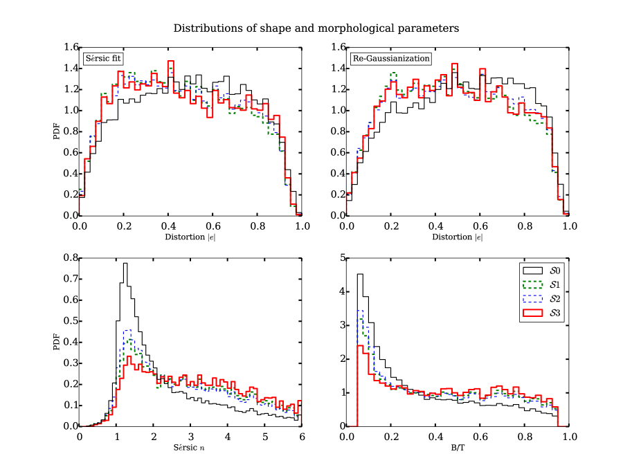
Fig. 5 shows the distribution of these morphological and shape parameters for the flux-limited sample $\mathcal{S}$$0$ and the three volume-limited samples - $\mathcal{S}$$1$, $\mathcal{S}$$2$ and $\mathcal{S}$$3$. In addition to the basic value in characterizing these distributions for our sample overall, it is also useful to understand how the samples change when we vary our method of volume-limiting the sample. For instance, galaxies with lower Sérsic indices are preferentially selected in $\mathcal{S}$$2$ compared to $\mathcal{S}$$1$ and $\mathcal{S}$$3$. Similarly, galaxies with low ellipticity/distortion values are rejected in generating $\mathcal{S}$$2$ (despite the lack of any explicit cut on shapes) while they are retained in $\mathcal{S}$$1$ and $\mathcal{S}$$3$. A simple explanation is that the cuts in $\mathcal{S}$$2$ are preferentially removing early-type populations, which have higher Sérsic indices and lower ellipticities. For example, if the luminosity evolution that was adopted is too strong particularly for early type populations, that could give rise to the effect shown in Fig. 5.

4 Results

Having identified the overdense and underdense regions in a volume-limited sample (Secs. 3.1 and 3.2), we will now see whether the morphological parameters of the galaxies described in Sec. 3.3 depend noticably on the environment of the redshift slice in which they reside. Note that for true 3D overdensities there is already substantial evidence in the literature that we should see variation of properties with the environment. Our test is necessary to see whether such morphology-density correlations are evident in the kind of 1D redshift slices that would be used for constructing weak lensing simulations, or whether our use of an area as large as the size of COSMOS will wash out these trends (which would be good news for weak lensing simulations based on that dataset).

As described in Sec. 3.2, we have three different ways of volume-limiting our sample:

1. no redshift evolution of luminosity cut $(\mathcal{S}1)$,

2. using $B$-band luminosity evolution applied to the $I$-band luminosities $(\mathcal{S}2)$, and

3. impose stellar mass cuts instead of luminosity $(\mathcal{S}3)$.

We will present our results in all three cases to check for their robustness to how the sample is selected.

4.1 Axis ratios

We can test the influence of environment on the galaxy shapes by comparing the distributions of the axis ratios for the overdense and underdense redshift slices, or by encapsulating that distribution as a single number, the RMS (root mean squared) ellipticity or distortion. By volume-limiting the sample, we have avoided issues wherein the flux limit leads to artificial changes in the sample as a function of redshift. We will also carry out tests to differentiate between environmental effects versus evolution of the population with redshift (at fixed mass).

4.1.1 Comparing distributions

Figure 6: The distributions of axis ratios of galaxies in all overdense (OD) and all underdense (UD) regions in the case of the luminosity-selected sample $\mathcal{S}$1 (left), luminosity-selected sample with $B$-band evolution taken into account $\mathcal{S}$2 (center), and thestellar-mass-selected sample $\mathcal{S}$3 (right). The upper panels show the histograms, and the bottom panels show the cumulative distribution functions (CDF). The $p$-values computed using these CDFs are shown in Table. 2.

Figure 7: Galaxy axis ratio distributions in two overdense redshift bins, $z=0.65-0.75$ (blue, dotted) and $z=0.80-0.85$ (red, solid), to check for consistency in the case that the environment is the same even if the redshift differs. The $p$-values from the KS and AD tests are given in Table. 2.

Figure 8: Galaxy axis ratio distributions in a single underdense redshift slice, $z=0.55-0.65$ (blue, dotted), and a single overdense redshift slice, $z=0.65-0.75$ (red, solid). The $p$-values from the KS and AD tests are given in Table. 2.

Redshift bins	$\mathcal{S}$$1$	$\mathcal{S}$$2$	$\mathcal{S}$$3$
All overdense vs.	$1.1\times 10^{-4}$	$2.6\times 10^{-5}$	$1.9\times 10^{-6}$
All underdense	$1\times 10^{-5}$	$<1\times 10^{-5}$	$<1\times 10^{-5}$
$[0.65,0.75]$ (OD) vs.	0.61	0.43	0.23
$[0.80,0.85]$ (OD)	0.49	0.24	0.13
$[0.65,0.75]$ (OD) vs.	$5.8\times 10^{-4}$	$1.5\times 10^{-5}$	$3.5\times 10^{-6}$
$[0.55,0.65]$ (UD)	$9.8\times 10^{-4}$	$<1\times 10^{-5}$	$<1\times 10^{-5}$

Table 2: $p$-values from the Kolmogorov-Smirnov (top) and Anderson-Darling (bottom) tests obtained by comparing the distributions of axis ratios for three cases: all overdense (OD) vs. all underdense (UD), two overdense bins that are not very separated in redshift, and a pair of adjacent overdense and underdense bins. $\mathcal{S}$$1$, $\mathcal{S}$$2$, $\mathcal{S}$$3$ refer to the three different types of volume-limited samples. The Anderson-Darling $p$-values are computed only up to 5 decimal places, so values that were given as zero are denoted $<1\times 10^{-5}$.

Redshift bins	$\mathcal{S}$$1$	$\mathcal{S}$$2$	$\mathcal{S}$$3$
All overdense vs.	$5.6\times 10^{-4}$	$1.0\times 10^{-4}$	$3.3\times 10^{-6}$
All underdense	$3\times 10^{-5}$	$1\times 10^{-5}$	$<1\times 10^{-5}$
$[0.65,0.75]$ (OD) vs.	0.96	0.75	0.54
$[0.80,0.85]$ (OD)	0.52	0.34	0.23
$[0.65,0.75]$ (OD) vs.	$6.0\times 10^{-3}$	$2.5\times 10^{-4}$	$2.4\times 10^{-4}$
$[0.55,0.65]$ (UD)	$1.2\times 10^{-2}$	$2.5\times 10^{-4}$	$5\times 10^{-5}$

Table 3: $p$-values from the Kolmogorov-Smirnov (top) and Anderson-Darling (bottom) obtained by comparing the second moments-based distortion for the same three cases as in Table 2. The Anderson-Darling $p$-values are computed only up to 5 decimal places.

We begin by comparing the entire axis ratio distributions $p(q)$ between pairs of redshift slices. Unless otherwise mentioned, the axis ratios refer to the values obtained using the method of Lackner & Gunn (2012) to fit single Sérsic profiles to each galaxy image. To compare the distributions and make statistical statements about their consistency, we use two statistical tests, the Kolmogorov-Smirnov (KS) test and Anderson-Darling (AD) test, the latter of which is carried out using the adk package in R.

We first compare the distribution of galaxy axis ratios in all overdense bins against that for all underdense bins in Fig. 6, with different panels showing the comparison for $\mathcal{S}$1, $\mathcal{S}$2, and $\mathcal{S}$3. The cumulative distribution functions are also shown, since they form the basis for our statistical statements about consistency using the KS and AD tests. The results of these tests are shown in the first two rows in Table 2. For all three ways of volume-limiting the sample, the $p$-values from both the KS and AD tests are well below 0.05 (a maximum of $1.1\times 10^{-4}$, but often smaller than that). We can therefore reject the null hypothesis that the overdense and underdense regions have the same underlying axis ratio distributions at high significance.

One might imagine that the disagreement between the distributions is, at least partly, due to the fact that the overdense and underdense sample have different redshift distributions and there could be some evolution of ellipticity/distortion distributions with redshift. To show that this redshift evolution effect is subdominant to environmental effects, we will compare distributions between pairs of two overdense (or pairs of underdense) redshift slices, where we expect to find similarity even if the redshifts are different if the environmental effects dominate. We will also compare between overdense and underdense regions that are selected to be nearby in redshift, so that any redshift evolution effects should be minimal. Figures 7 shows that the axis ratio distributions are indeed consistent when the environments are similar but the redshifts are different. Likewise Fig. 8 shows that for adjacent redshift slices with different environments, the axis ratio distributions are inconsistent. The results of statistical tests for the distributions in these figures are given in Table 2, and support our statement that the morphology-density correlation is the dominant effect when comparing overdense and underdense redshift slices, with redshift evolution of the population being negligible. Comparing other pairs of redshift bins leads to similar conclusions.

Finally, we can check whether these findings are particular to the axis ratios from the Sérsic fits, or whether we reproduce this finding when we use the shapes from the centrally-weighted moments-based re-Gaussianization method, which estimates a distortion (Eq. 8) for each galaxy. After neglecting a small fraction ($<0.01$ per cent) of galaxies for which the method does not converge, we carry out the same statistical tests from Table 2, but using the moments-based shape estimates. The results of the KS and AD tests are tabulated in Table 3. We see that all of our findings with the Sérsic fit-based shapes carry over to shapes from a centrally-weighted moments-based shape estimate.

4.1.2 RMS distortions

Figure 9: RMS distortions as a function of redshift. The horizontal errorbars indicate the width of the redshift bin, while the vertical ones are $1\sigma$ errorbars obtained by bootstrapping. The colours and shapes of the points indicate their environmental classification, as shown in the legend. Points with open centers and thick errorbars correspond to the stellar-mass selected sample $\mathcal{S}$$3$ and points with filled centers and thin errorbars correspond to the luminosity-selected samples $\mathcal{S}$$1$ and $\mathcal{S}$$2$.

Figure 10: RMS distortions as a function of redshift, with points defined in a similar way as in Fig. 9. In this case, the distortions from moments-based shape estimates, rather than from the Sérsic fits.

We can also carry out tests on a single statistic of the galaxy shape distribution in each redshift slice, like the RMS distortion. While tests of a single quantity may seem less powerful than tests that use the entire shape distributions, the advantage is that instead of picking out pairs of redshift slices for our tests, we can easily compute our statistic of interest for every single redshift slice, and look for trends with both redshift and environment.

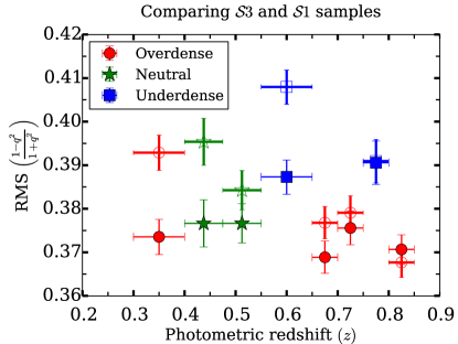
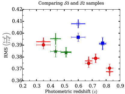
For the luminosity-selected samples ($\mathcal{S}$$1$, $\mathcal{S}$$2$), the RMS distortions (Eq. 8) of galaxies in each redshift bin are shown in Fig. 9. In each case, the RMS distortions from the mass-selected sample ($\mathcal{S}$$3$) are also plotted. When the $B$-band luminosity evolution is taken into account in selecting the sample, a systematic increase in the distortion values at lower redshifts can be observed (bottom panel).The stellar-mass selected sample exhibits a similar trend.

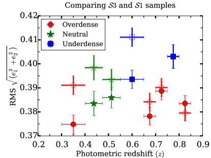
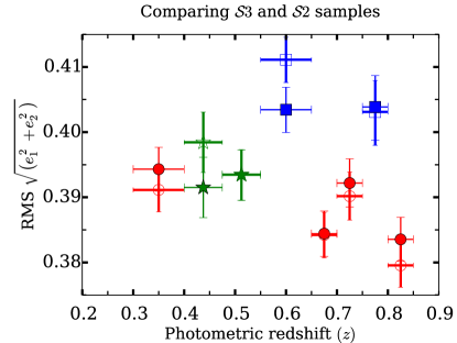
For figures up to Fig. 12, the colours of the points were selected to easily differentiate between galaxies in overdense, neutral, and underdense redshift slices. Points with unfilled centers and thicker errorbars correspond to the $\mathcal{S}$$3$ sample and points with filled centers and thinner errorbars correspond to the luminosity-selected samples ($\mathcal{S}$$1$ or $\mathcal{S}$$2$).

As shown in Fig. 9, the underdense regions have higher values for RMS distortions when compared to the overdense regions. The difference between the underdense and overdense regions for $z>0.5$ is significantly larger than any redshift evolution across the $z>0.5$ range. Our conclusions are very similar if we use the RMS ellipticity from Eq. (9) instead of the distortions.

The sign of the dependence on the local environment is reasonable when compared with previous work on the morphology-density relation (see, e.g. van der Wel et al., 2010). Overdense regions typically contain many old, elliptical galaxies which are close to round (large axis ratio and low RMS ellipticity/distortion). In contrast, the underdense regions typically contain a larger population of younger, disk galaxies, which have lower axis ratios and higher RMS ellipticity/distortion.

From Figs. 1 and 4, the $0.4\leq z<0.55$ redshift range shows signs of being marginally underdense, but has low RMS ellipticity that agrees with the rest of the overdense regions.

Next, we show an analogous plot of RMS distortions for all three volume-limited sample using the moments-based shape estimates in Fig. 10. The conclusions are quite similar to those using the shapes from the Sérsic profile fits, with the underdense regions standing out in having larger RMS distortions than the other redshift slices, an effect that is substantially larger than any average redshift evolution of the RMS distortions.

However, the statistical significance of trends in this section using a single statistic of the shape distribution (the RMS) is less than the significance of the trends seen using the entire axis ratio distributions in Sec. 4.1.1.

Finally, we comment on whether the trends we have found could be caused by measurement noise rather than variations in the intrinsic shape distributions. Measurement error tends to cause an increase in the RMS ellipticity due to the broadening of the measured ellipticity distributions. However, this is one of the reasons we restricted the sample to a magnitude of 23.5. In this case, the $S/N$ of the flux measured in the galaxy images is typically $\geq 50$. If we consider the worst case, i.e., assume all galaxies have $S/N=50$ and use the Gaussian approximation from Bernstein & Jarvis (2002), the expected measurement error on the distortion is $0.08$. If we add this in quadrature with an RMS of $\sim 0.33$, then the new RMS becomes $0.34$. However, we see variations in the RMS distortion in different environments that are as large as $0.05$, or five times as large as this worst-case scenario due to measurement noise. Moreover, if measurement error were a significant issue, we would expect it to affect the comparison of (for example) low- and high-redshift samples in overdense regions. In a volume-limited sample, those will have different flux distributions and therefore different SNR distributions. However, there is little trend in the RMS distortion with redshift for overdense regions, which suggests empirically that measurement error is not a significant factor in our results.

4.2 Morphological parameters

For the morphological parameters that we described in Sec. 3.3, the Sérsic index and bulge-to-total ratio, we do not compare the distributions directly. Doing so is relatively difficult because both distributions have hard cutoffs that are enforced in the fitting process (Sérsic $n$ in the range $[0.25,6]$ and $0.05<B/T<0.95$), as can be seen in Fig. 5. The KS statistical test is sensitive to exactly what happens at these hard boundaries in the distributions. So, instead of using the full distributions, we will study the dependence of these quantities on environment by computing the median values in different redshift slices. Median values are preferred over the full distributions or even the sample means since the medians are more robust to what happens at the edges of the distributions.

Fig. 11 shows the median value of the Sérsic index in each redshift slice, with and without taking into account of luminosity evolution when volume-limiting the samples ($\mathcal{S}$1 and $\mathcal{S}$2). Both panels also show the results with stellar mass-selected samples ($\mathcal{S}$3) for reference. When using the stellar mass-selected sample, we observe that the overdense regions tend to have higher Sérsic index than the underdense ones, with the redshift evolution being mild and the results for the underdense regions particularly standing out. This trend is consistent with our previous explanation for trends in RMS ellipticities; the underdense regions have more spiral galaxies and therefore a lower median value of Sérsic $n$. However, this trend is less evident for the luminosity-selected samples, where there seems to be some evolution with redshift that dominates over the environmental effects.

We also note that in Fig. 11, the median Sérsic indices of the stellar mass-selected samples ($\mathcal{S}$$3$) are systematically greater than those of the luminosity selected samples ($\mathcal{S}$$1$, $\mathcal{S}$$2$). This is because $\mathcal{S}$3 is restricted to galaxies with masses above $\log(M/M_{\odot})>10.15$, whereas in $\mathcal{S}$1 and $\mathcal{S}$2, the mass distribution of galaxies extends to $\log(M/M_{\odot})\sim 9.0$, with about 44 per cent of the galaxies in $\mathcal{S}$2 having a stellar mass below the cut for $\mathcal{S}$3. It is therefore not surprising that $\mathcal{S}$3 has a higher median Sérsic $n$. Finally, even for the stellar mass-selected sample there is some sign of redshift evolution. The sign of this evolution is as expected, with lower Sérsic $n$ and $B/T$ for higher redshift samples, which should have a higher fraction of disk and irregular galaxies and fewer galaxies with bulge-like morphology.

Finally, Fig. 12 shows the variation of the median bulge-to-total ratio with redshift. The results are quite consistent with those of Fig. 11. Thus, our results in this section suggest that the environment can significantly affect the median morphological parameters of galaxies selected in thin redshift slices, assuming that the galaxies represent a stellar mass-selected sample. The trend is less evident when using luminosity to select the galaxies.

Figure 11: Median values of the Sérsic indices for volume-limited samples $\mathcal{S}$$1$ and $\mathcal{S}$$2$ are plotted (filled centers and thin errorbars) in top and bottom panels, respectively, for each redshift bin. Median values for the $\mathcal{S}$$3$ sample are plotted in both the panels (open centers and thick errorbars) in both the panels.

Figure 12: Median values of the bulge-to-total ratios for volume-limited samples $\mathcal{S}$$1$ and $\mathcal{S}$$2$ are plotted (filled centers and thin errorbars) in left and right panels respectively for each redshift bin. Median values for the $\mathcal{S}$$3$ sample are plotted in both the panels (open centers and thick errorbars). The horizontal errorbars simply correspond to the binwidth while the vertical ones are $1\sigma$ errorbars obtained by bootstrapping.

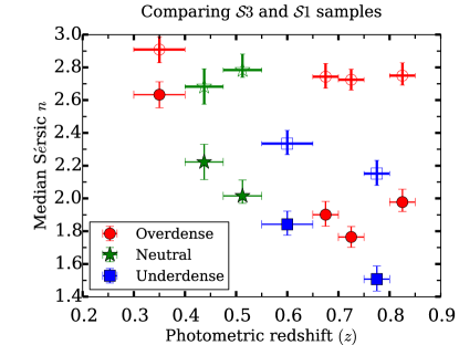
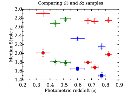
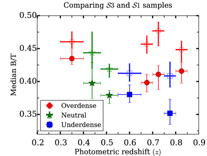
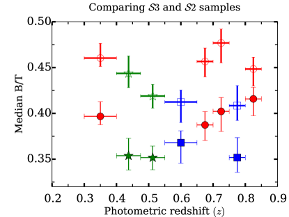
One might expect the points corresponding to neutral regions to lie in between the points for overdense and underdense regions. In Figs. 9–12, this does not always appear to be the case. It is possible that a redshift bin may have an overdensity in one part of the field and an underdense region in another. In such a scenario, the redshift slice might appear to be ‘neutral’ in our histogram-based method of finding overdensities, while still having significant large-scale structure affecting the morphological mix of galaxies that complicates the situation. This indeed turns out to be the case in the ‘neutral’ regions of the COSMOS field. Using X-ray information in the COSMOS field, Leauthaud et al. (2010) have detected several galaxy groups in the redshift range $z=0.425-0.575$. Kovač et al. (2010) report structures that are large and extended (in RA-DEC) within this redshift range. It is a challenge to make definitive statements regarding the relationship between environment and morphology in neutral regions that are composed of mixtures of multiple overdense and underdense regions. In addition, the redshift evolution, albeit weak, can make the neutral bins look like overdense or underdense regions. For instance, the neutral bins look overdense-like in Figs. 9-11 but underdense-like in Fig. 12, partly due to redshift evolution. However, when the overdensity (or underdensity) is prominent, we observe that the environment in which a galaxy resides affects its morphology, so the appearance of the neutral bins does not undermine the main conclusions of this paper.

To test the possibility that our choice of bins starting at $z=0.3$ with $\Delta z=0.05$ is particularly unlucky in enhancing the effects we see, we carried out the same analysis using bins of the same width but shifted by $\Delta z/2$. We recomputed the overdensities keeping the parameters of the redshift distributions same as before. Shifting the bins enhances the overdensities and underdensities in some cases and in other cases, it mixes the overdense and underdense regions to make them more neutral-like. The environmental trends still are observed in the enhanced bins and hence our conclusions are still applicable.

The number of galaxies in overdense bins is typically higher than the number in underdense bins by about a factor of 2. (See Table  1). To eliminate the possibility (with great confidence) that this varying sample size is responsible for the trend observed, we repeated our analysis with only 50 per cent of overdense galaxies that were selected randomly. The vertical errorbars for overdense regions get bigger due to reduced sample size, but the statistical significance of our conclusions is still nearly as high as in the original analysis.

4.3 Mitigating the effects of line of sight fluctuations

Figure 13: Plot of $\delta_{g,\text{1D}}=N/N_{\text{mod}}-1$ with each functional form as the model for each of our new wide redshift bins discussed in Sec. 4.3, for flux-limited (top) and volume-limited (bottom) samples.

Figure 14: Median values of Sérsic index, as a function of redshift for our wider redshift ranges used in Sec. 4.3. The horizontal errorbars indicate the width of the redshift bin, while the vertical ones are $1\sigma$ errorbars obtained by bootstrapping. Points with open centers and thick errorbars correspond to the stellar-mass selected sample $\mathcal{S}$$3$ and points with filled centers and thin errorbars correspond to the luminosity-selected samples $\mathcal{S}$$1$ and $\mathcal{S}$$2$.

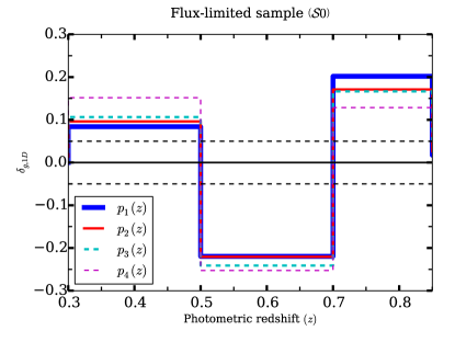
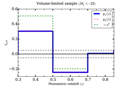
Since we have argued that cosmic variance is giving rise to environmentally-based variations between galaxy populations in our redshift slices that are $0.05$ wide, the natural question is how to mitigate this effect so that it will not affect attempts to simulate a realistic galaxy sample as a function of redshift. The most obvious approach is to repeat the analysis with wider redshift bins. Feigning ignorance of overdensities and underdensities along the line of sight, we choose the slices in redshift to be $\left[0.3-0.5\right]$, $\left[0.5-0.7\right]$ and $\left[0.7-0.85\right]$ (a nearly even division of our entire redshift range) and redo the analysis, beginning by checking the environmental classification for these wide bins.

Using the redshift distributions estimated earlier in this work (cf. Figs. 1 and 4), we obtain the overdensity estimates for the wider bins, $\delta_{g,\text{1D}}$. Although the $\left[0.7-0.85\right]$ bin seems to be overdense in the top panel of Fig. 13, it appears to be environmentally neutral when we volume-limit the sample using the methods from Sec. 3.2. Since the latter is what we use to study the galaxy morphology, we classify $\left[0.7-0.85\right]$ bin as ‘neutral’. What is surprising is the fact that the lowest and middle redshift slices still qualify as substantial overdensities and underdensities despite our use of $\Delta z=0.2$.

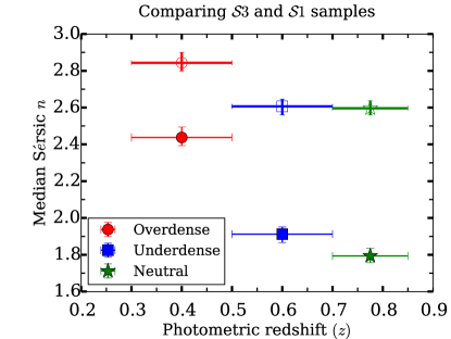
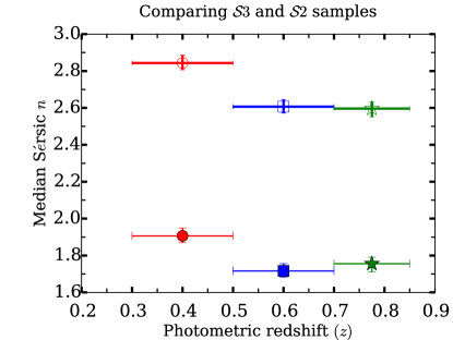
As an example of what happens to morphological parameters, we show the median Sérsic index for three bins in Fig. 14. Comparing this with Fig. 11, we observe that the range of Sérsic $n$ values has become smaller, as have the vertical errorbars, mainly due to the increase in the number of galaxies in each redshift bin. The results do not suggest that the values are consistent across all redshift bins, and in particular, the disparity between overdense and underdense regions is still quite evident (with the same sign as before). However, in Fig. 11, the magnitude of that disparity between overdensities and underdensities was around 20 per cent, whereas here it is reduced to 7 per cent. This seems to suggest that when we choose wider redshift bins, some of the large-scale structure gets washed out, so the galaxy morphological parameters are less affected by cosmic variance. This is a promising result, which could be further improved by either (a) non-blind selection of the wide redshift bins with respect to known structure in the calibration fields, or (b) attempting some kind of reweighting of the galaxy populations in redshift slices affected by known structure.

As a test of the second option, we consider whether we can use some division of the galaxies by colour or $B/T$ (as a proxy for colour) in order to determine the structural parameters of galaxies as a function of redshift for each of them separately. If the effects we are seeing can be cleanly described in terms of overdense (underdense) regions being dominated by bulge- (disk-)dominated galaxies, then division into samples based on $B/T$ may help reduce the effects that we have described in previous subsections. We test this idea by dividing the sample into bulge- and disk-dominated galaxies based on requiring $B/T\geq$ or $<0.5$. The resulting bulge fraction $f_{\text{bulge}}$, shown as a function of redshift in Fig. 15, shows a mild effect from the large-scale structures in the COSMOS field.

Figure 15: The fraction of galaxies in $\mathcal{S}$1 (solid symbols) and $\mathcal{S}$3 (open symbols) that are classified as bulge-dominated as a function of redshift, including the correlation with redshift slices classified as overdense or underdense as indicated by the symbol shape and colour.

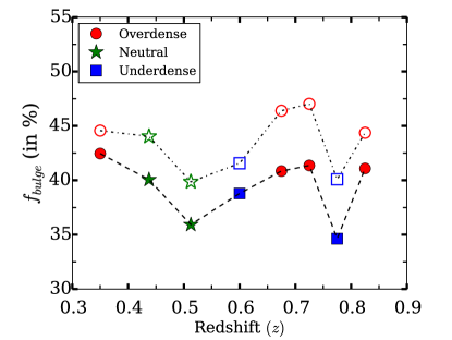
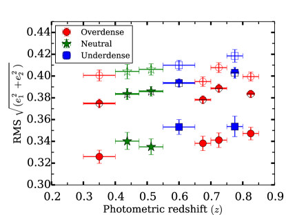
Fig. 16 shows the RMS distortion as a function of redshift for the full $\mathcal{S}$1 sample (as shown previously) and for the separate bulge- and disk-dominated samples. As shown, the deviations in the values due to large-scale structure are clearly evident in all three cases, though slightly more prominent for the full sample and less so for the bulge-dominated sample. For comparison with the results for the full sample shown in Table 2, we compute the KS (AD) test $p$-values for consistency of axis ratios between overdense and underdense regions for bulge- and disk-dominated samples. For $\mathcal{S}$1, these $p$-values are 0.16 (0.08) for bulge-dominated galaxies and 0.005 (0.001) for disk-dominated galaxies. For $\mathcal{S}$3, these $p$-values are 0.03 (0.03) and $10^{-4}$ ($3\times 10^{-4}$), respectively. With the possible exception of bulge-dominated galaxies, it seems that separation into two morphological samples is not enough to remove the effect of the local environment on the ensemble properties like the intrinsic ellipticity distribution. Due to the limited sample size, we did not explore the possibility of an even finer morphological division of the sample, but with deeper HST datasets, this may be a promising path to pursue. However, if the nature of the bulges or disks themselves is altered by the local environment, then division purely into bulge- or disk-dominated sample will not be helpful in mitigating environmental effects.

Figure 16: The RMS distortion as a function of redshift for the full volume-limited galaxy sample $\mathcal{S}$3 (partially-full symbols), the disk-dominated galaxy sample (open symbols), and the bulge-dominated galaxy sample (full symbols). The fact that the bulge-dominated sample has a lower RMS distortion than the disk-dominated sample is consistent with expectations.

5 Implications for future surveys

As mentioned previously, HST data will be used by current and future weak lensing surveys to characterize the galaxy population in several ways. In this section, we estimate how the results shown in Sec. 4 can affect estimates of shear calibration when using HST to characterize the galaxy population. We also discuss the situations in which this is likely to be important for current and future surveys from the space and ground.

5.1 Magnitude of shear calibration bias

Here we consider the impact of the findings in Sec. 4 on weak lensing shear calibration assuming that the COSMOS sample is used as a parent sample for simulations that are used to derive redshift-dependent shear calibrations. This could be done either directly using the galaxy images themselves, or by fitting for parametric distributions of Sérsic $n$, size, and shape in redshift slices, and then using those parametric distributions to make simulated images containing galaxies with Sérsic light profiles that match those distributions. We consider a few simple cases of how the above results affect shear calibration estimates. It is likely that the answer to this question varies quite significantly with the type of shear estimation method used. Some will be sensitive to the variations in morphology, others to the variation in the intrinsic ellipticity distribution, and many will be sensitive to both at some level. We consider both of these issues in turn.

The intrinsic ellipticity distribution plays a role in nearly all shear estimators. In some, the role is explicit: for example, LensFit (Miller et al., 2007; Kitching et al., 2008; Miller et al., 2013) and the methods presented by Bernstein & Armstrong (2014) require accurate intrinsic ellipticity distributions as inputs, and uncertainty in the distribution was one source of systematic uncertainty in the CFHTLenS weak lensing results (Heymans et al., 2013; Miller et al., 2013). The intrinsic ellipticity distribution enters the calculation for other methods in other ways. For example, the re-Gaussianization method and several other moment-based methods require calculation of a shear responsivity (Bernstein & Jarvis, 2002; Hirata & Seljak, 2003) that describes how the galaxy population overall responds to a shear, based on its intrinsic ellipticity distribution. The responsivity can be calculated based on the observed shape distribution, assuming that the uncertainties in the shears are known well enough that their contribution to that distribution can be removed. If a simulated sample in some redshift slice has a different intrinsic ellipticity distribution and therefore responsivity, it could lead to incorrect conclusions about shear calibration. The responsivity scales roughly like $1-e_{\text{RMS}}^{2}$, which means that deviations in RMS distortion at the level of 0.01 due to local environments (Figs. 9 and 10) would become fractional shear errors of

$$\frac{\Delta\gamma}{\gamma}\approx\frac{2e_{\text{RMS}}\Delta e_{\text{RMS}}}{1-e_{\text{RMS}}^{2}}\approx 0.01.$$ (11)

In the context of upcoming lensing surveys that seek to constrain shears to better than the per cent level, a systematic error of this magnitude in shear calibration is quite serious.

Regarding possible biases in the morphological mixtures of galaxies due to overdensities or underdensities in the training sample, there are results in the literature for several methods that show how shear biases vary with morphology. For example, for the maximum likelihood fitting code im3shape, figure 2 in Kacprzak et al. (2012) shows multiplicative biases for two-component Sérsic profile galaxies as a function of their bulge-to-total ratios (denoted there as $F_{b}/(F_{b}+F_{d})$, which we will equate with our $B/T$). The shear calibration bias scales roughly like $0.04-0.05(B/T)$ as $B/T$ goes from $0$ to $1$. Our results suggest that typical (median) $B/T$ values may be influenced by cosmic variance in the COSMOS field, leading to fluctuations of order $0.05$. The resulting variation in the shear calibration would therefore be $\sim 2.5\times 10^{-3}$, or $0.25$ per cent shear calibration uncertainty. For existing datasets this is not very problematic, but for surveys like LSST, Euclid, and WFIRST-AFTA, this would be a dominant part of the systematic error budget. As another example, for re-Gaussianization, figure 9 of Mandelbaum et al. (2012) shows that as Sérsic $n$ goes from $1$ to $6$, the shear calibration bias varies by $2$ per cent. In this case, since we have shown that the median value of Sérsic $n$ can vary by $\sim 0.4$ due to morphology-density correlations, this suggests that the shear calibration for re-Gaussianization could be misestimated by $\sim 2\times 10^{-3}$, or 0.2 per cent. This too is acceptable in existing datasets, but not those that will be used for shear estimation in the next decade.

The estimates in this subsection are rough illustrations of the magnitudes of these effects. Other aspects of shear calibration that could be affected relate to the use of HST data to estimate the impact of detailed galaxy morphology, or to calibrate the effect of colour gradients (Voigt et al., 2012; Semboloni et al., 2013). In the latter case, what is most relevant in this work is our finding that $B/T$ exhibits environmental dependence, which likely translates into environmental dependence of colour gradients. Unfortunately, we cannot directly test the strength of any colour gradient variations with environment using COSMOS data, due to the fact that there is only single-band coverage in much of its area. We note that our findings may seem to be at odds with the conclusions in Semboloni et al. (2013) based on synthetic galaxy models that the existing area of HST coverage with $\geq 2$ bands is sufficient for calibration of colour gradients. This is particularly striking given that, as shown there, the dominant galaxy sample with $2$-band coverage is the AEGIS dataset, which has substantially smaller area than COSMOS, and therefore should exhibit a stronger influence of cosmic variance. The presence of other fields besides AEGIS (e.g., GOODS) should help mitigate this effect given that the large-scale structure in the two fields will be completely uncorrelated, but the number of fields is still not large and the area is dominated by a small number of them.

However, it is important to bear in mind that the method proposed in Semboloni et al. (2013) involves determining not just a redshift-dependent correction but also a type-dependent colour gradient correction, which could partially mitigate the effects of the environment dependence seen here. Moreover, the colour gradient effect is higher order than the intrinsic ellipticity distribution, and thus may be less susceptible to systematics due to the environmental effects considered here. We showed in Sec. 4.3 that a simple type-dependent split does not remove the effects of environment on the intrinsic ellipticity distribution, but testing whether it (or a more complex type or colour split) is enough to remove the effects of colour gradients in Euclid is a more complicated analysis that is beyond the scope of this work. It seems that a future study using an HST field with more than one band would be warranted, to test whether or not our results suggest a discrepancy with those of Semboloni et al. (2013). It is possible that the connection between colour gradients and $B/T$ is weak enough that our results do not imply a problem with colour gradient calibration, or that division into several galaxy types or colours is truly enough to remove the colour gradient effect due to its being a higher order effect, consistent with the findings of Semboloni et al. (2013) using synthetic galaxy models.

5.2 Effective impact on current and future surveys

In addition to the order of magnitude of these effects presented in the previous subsection, it is important to bear in mind how current and future surveys plan to use HST data.

For example, before the Euclid survey begins, when carrying out tests of shear estimation methods, their simulated data will be based on HST in many ways: estimation of simple aspects of morphology (Sérsic $n$, bulge fraction), intrinsic ellipticity distribution, colour gradient calibration, and higher order moments (detailed morphology). Our results suggest that care should be taken to ensure that those simulations are not overly influenced by environment effects in the HST data, so that incorrect conclusions will not be drawn about the redshift-dependence of shear calibration for shear estimation methods to be used by the survey.

However, once the Euclid survey is underway, the derivation of simple galaxy morphology and the intrinsic ellipticity distribution will be based on the 40 deg² Euclid deep field, which goes two magnitudes fainter than the rest of the survey. With that data in hand, the Euclid weak lensing results will be less reliant on the much smaller and more cosmic variance-limited HST fields, using them only for colour gradient calibration and estimates of the impact of detailed galaxy morphology (since the HST resolution is higher than that of Euclid). The findings of Viola, Kitching & Joachimi (2014) demonstrate that the area of this deep field is sufficient to accomplish the goal of determining the intrinsic ellipticity distribution at the accuracy required for shear calibration purposes for the Euclid survey.

In contrast, for ground-based surveys such as LSST, high-resolution space data will play a more important role in the understanding of the galaxy intrinsic ellipticity and morphology distributions, since even a deep field in a ground-based survey faces fundamental resolution limits that prevent the derivation of detailed information about the faint galaxy population. Galaxies that are near the resolution limit for a ground-based survey are still very well-resolved in HST, making it the best resource for detailed information about them. Once the Euclid deep field is publicly available, the information from it will be beneficial to ground-based surveys as well.

Finally, our results for the effect on the intrinsic ellipticity distributions suggest that even current surveys should be careful to avoid this effect. While use of COSMOS without accounting for the effect that we have identified will cause a bias that is similar to the final requirements on the shear systematic errors for Stage III surveys, there are other elements in the systematic error budget, so ideally this effect should be mitigated somewhat using, for example, the wider redshift binning strategy that we tested in Sec. 4.3. Use of significantly smaller fields than COSMOS, while possibly helpful in building up a deeper galaxy sample, should naturally increase the impact of cosmic variance on the training dataset, which should be quantified as part of the systematic error budget.

6 Conclusions

In this study, we have shown that the shape distributions of galaxies (to a statistically significant degree) and morphological parameters like Sérsic $n$ and bulge-to-total ratios (more marginally) depend on the local environments when dividing up the COSMOS sample into redshift slices along the line of sight. The redshift slices used for our primary analysis had a width of $\Delta z=0.05$. Our findings are robust to the choice of shape estimator from Sérsic profile fits vs. using centrally weighted moments-based shear estimates.

These findings are relevant to attempts to use HST-based galaxy samples to calibrate shear estimates in weak lensing surveys. In general, the approach would be to define galaxy samples using all galaxies in redshift slices, and determine a redshift-dependent shear calibration. Our findings highlight the danger in such an approach: while we would like our simulations to include true evolution in galaxy properties with redshift, this approach also includes spurious variations in galaxy properties due to the large-scale structure within the COSMOS field. Since the fidelity of weak lensing shear estimates depends sensitively on the intrinsic shape distribution and galaxy morphological parameters, the conclusions for the redshift-dependent shear calibration would be incorrect. As shown in Sec. 4.3, these errors are reduced as the redshift slices that are used become wider, so that the impact of local overdensities becomes washed out. However, our results suggest that even $\Delta z=0.2$ may not be wide enough (and this is becoming dangerously close to the size of tomographic redshift bins to be used for weak lensing analysis in upcoming surveys). Thus, more complex schemes may become necessary to fully overcome this issue, depending on exactly how the HST data is to be used. As discussed in Sec. 5, particular care may be needed in ground-based surveys that will use the HST data to model many aspects of the galaxy population. In contrast, for Euclid, use of the relatively large area Euclid deep data to constrain many aspects of the galaxy population means that these issues with HST data are less important, though still not completely ignorable.

It is important to keep in mind the nature of COSMOS with respect to other possible HST training samples. COSMOS represents the largest contiguous field surveyed by the HST, with the sizes of other major HST fields such as GOODS and AEGIS lagging by at least a factor of 9 (for AEGIS, and more for GOODS). Combinations of CANDELS with existing datasets may ultimately be as large as $1/6$ the COSMOS area. Hence, if cosmic variance due to structures along the line of sight in COSMOS are problematic for its use as a training sample for weak lensing simulations, studies that use even smaller area training samples are even more prone to errors, with the UDF serving as an extreme case. If the size of the HST survey is small enough, there is no reason a priori to suppose that the galaxy population is typical even when using all galaxies along the line of sight, without any division into redshift bins. Of course, future surveys are unlikely to pick just a single survey to serve as the basis for their image simulation training sample, but rather will combine as many as possible. Combining multiple surveys will reduce the cosmic variance and therefore the significance of the effects discussed in this work. However, as COSMOS is significantly larger than other HST surveys, combining COSMOS with smaller fields is unlikely to ameliorate this effect. Thus, it will be important to carefully choose the size of redshift slices used to derive properties of the galaxy population so as to be minimally affected by this issue.

A final consideration is the question of how applicable these results using volume-limited samples are to simulations of upcoming weak lensing surveys, which will exclusively use flux-limited samples. For our analysis, the volume-limiting sample was necessary to avoid complications due to varying galaxy populations in each redshift slice, allowing us to isolate purely environmental effects. In principle, if the morphology-density correlations that we have identified turn out to not exist for intrinsically fainter galaxy populations, then at low redshift (where a flux limited sample will include galaxies that are intrinsically much fainter than at high redshift), the effects will be less serious for upcoming lensing surveys. However, we do not have any particular reason to believe that these effects will vanish for fainter galaxies. Moreover, at higher redshift where only intrinsically bright galaxies can be seen, the effect should be present at a level similar to what we have found here. Since higher redshift galaxies tend to dominate cosmological shear estimates (due to their higher shears), our findings will be important to take into account. It would also be advisable to carry out a future study of this effect at higher redshift (beyond $0.85$), using for example the data from the CANDELS survey.

In conclusion, our results have serious implications for the plans to create realistic image simulations that will be used to derive redshift-dependent shear calibrations for upcoming weak lensing surveys. If care is not taken to mitigate this effect, then the cosmic variance in the training sample may bias the conclusions regarding shear calibration for redshift slices that represent significant overdensities or underdensities compared to the typical galaxy population. This is particularly a problem when using the smaller HST surveys, where a single galaxy cluster or a void could completely dominate the galaxy population in a given redshift slice. To mitigate this problem, it will be imperative to (a) collect training data from widely separated patches on the sky, and (b) take care to use redshift slices that are broad enough that these effects are reduced, so as to wash out the effect of any signal overdensity or underdensity on the simulated galaxy population. By employing these mitigation schemes, there is every reason to believe that the effect we have identified can be reduced to a small component of the systematic error budget of major upcoming lensing surveys.

References

- Albrecht et al. (2006) Albrecht A. et al., 2006, preprint (arXiv:astro-ph/0609591)
- Bartelmann & Schneider (2001) Bartelmann M., Schneider P., 2001, Phys.Rep., 340, 291
- Bernstein (2010) Bernstein G. M., 2010, MNRAS, 406, 2793
- Bernstein & Armstrong (2014) Bernstein G. M., Armstrong R., 2014, MNRAS, 438, 1880
- Bernstein & Jarvis (2002) Bernstein G. M., Jarvis M., 2002, AJ, 123, 583
- Blanton et al. (2003) Blanton M. R. et al., 2003, ApJ, 592, 819
- Bridle et al. (2010) Bridle S. et al., 2010, MNRAS, 405, 2044
- Bruzual & Charlot (2003) Bruzual G., Charlot S., 2003, MNRAS, 344, 1000
- Bundy et al. (2006) Bundy K. et al., 2006, ApJ, 651, 120
- Carollo et al. (2014) Carollo C. M. et al., 2014, preprint (arXiv:1402.1172)
- Chabrier (2003) Chabrier G., 2003, PASP, 115, 763
- Coil et al. (2004) Coil A. L., Newman J. A., Kaiser N., Davis M., Ma C.-P., Kocevski D. D., Koo D. C., 2004, ApJ, 617, 765
- de Jong et al. (2013) de Jong J. T. A. et al., 2013, The Messenger, 154, 44
- De Propris et al. (2014) De Propris R. et al., 2014, MNRAS, 444, 2200
- Faber et al. (2007) Faber S. M. et al., 2007, ApJ, 665, 265
- Giallongo et al. (2005) Giallongo E., Salimbeni S., Menci N., Zamorani G., Fontana A., Dickinson M., Cristiani S., Pozzetti L., 2005, ApJ, 622, 116
- Green et al. (2012) Green J. et al., 2012, preprint (arXiv:1208.4012)
- Heymans et al. (2013) Heymans C. et al., 2013, MNRAS, 432, 2433
- Hirata & Seljak (2003) Hirata C., Seljak U., 2003, MNRAS, 343, 459
- Ilbert et al. (2009) Ilbert O. et al., 2009, ApJ, 690, 1236
- Jee et al. (2013) Jee M. J., Tyson J. A., Schneider M. D., Wittman D., Schmidt S., Hilbert S., 2013, ApJ, 765, 74
- Kacprzak et al. (2012) Kacprzak T., Zuntz J., Rowe B., Bridle S., Refregier A., Amara A., Voigt L., Hirsch M., 2012, MNRAS, 427, 2711
- Kaiser et al. (2010) Kaiser N. et al., 2010, in Society of Photo-Optical Instrumentation Engineers (SPIE) Conference Series, Vol. 7733, Society of Photo-Optical Instrumentation Engineers (SPIE) Conference Series
- Kitching et al. (2012) Kitching T. D. et al., 2012, MNRAS, 423, 3163
- Kitching et al. (2008) Kitching T. D., Miller L., Heymans C. E., van Waerbeke L., Heavens A. F., 2008, MNRAS, 390, 149
- Koekemoer et al. (2007) Koekemoer A. M. et al., 2007, ApJS, 172, 196
- Kovač et al. (2010) Kovač K. et al., 2010, ApJ, 708, 505
- Kriek et al. (2009) Kriek M., van Dokkum P. G., Labbé I., Franx M., Illingworth G. D., Marchesini D., Quadri R. F., 2009, ApJ, 700, 221
- Lackner & Gunn (2012) Lackner C. N., Gunn J. E., 2012, MNRAS, 421, 2277
- Laureijs et al. (2011) Laureijs R. et al., 2011, preprint (arXiv:1110.3193)
- Leauthaud et al. (2010) Leauthaud A. et al., 2010, ApJ, 709, 97
- Leauthaud et al. (2007) Leauthaud A. et al., 2007, ApJS, 172, 219
- Lin et al. (1999) Lin H., Yee H. K. C., Carlberg R. G., Morris S. L., Sawicki M., Patton D. R., Wirth G., Shepherd C. W., 1999, ApJ, 518, 533
- LSST Science Collaboration et al. (2009) LSST Science Collaboration et al., 2009, preprint (arXiv:0912.0201)
- Mandelbaum et al. (2012) Mandelbaum R., Hirata C. M., Leauthaud A., Massey R. J., Rhodes J., 2012, MNRAS, 420, 1518
- Mandelbaum et al. (2014) Mandelbaum R. et al., 2014, ApJS, 212, 5
- Mandelbaum et al. (2013) Mandelbaum R., Slosar A., Baldauf T., Seljak U., Hirata C. M., Nakajima R., Reyes R., Smith R. E., 2013, MNRAS, 432, 1544
- Melchior et al. (2010) Melchior P., Böhnert A., Lombardi M., Bartelmann M., 2010, A&A, 510, A75
- Melchior & Viola (2012) Melchior P., Viola M., 2012, MNRAS, 424, 2757
- Miller et al. (2013) Miller L. et al., 2013, MNRAS, 429, 2858
- Miller et al. (2007) Miller L., Kitching T. D., Heymans C., Heavens A. F., van Waerbeke L., 2007, MNRAS, 382, 315
- Miyazaki et al. (2006) Miyazaki S. et al., 2006, in Society of Photo-Optical Instrumentation Engineers (SPIE) Conference Series, Vol. 6269, Society of Photo-Optical Instrumentation Engineers (SPIE) Conference Series
- Newman et al. (2015) Newman J. A. et al., 2015, Astroparticle Physics, 63, 81
- Refregier et al. (2012) Refregier A., Kacprzak T., Amara A., Bridle S., Rowe B., 2012, MNRAS, 425, 1951
- Rowe et al. (2014) Rowe B. et al., 2014, preprint (arXiv:1407.7676)
- Schrabback et al. (2010) Schrabback T. et al., 2010, A&A, 516, A63
- Scoville et al. (2007) Scoville N. et al., 2007, ApJS, 172, 1
- Semboloni et al. (2013) Semboloni E. et al., 2013, MNRAS, 432, 2385
- Semboloni et al. (2011) Semboloni E., Hoekstra H., Schaye J., van Daalen M. P., McCarthy I. G., 2011, MNRAS, 417, 2020
- The Dark Energy Survey Collaboration (2005) The Dark Energy Survey Collaboration, 2005, preprint (arXiv:astro-ph/0510346)
- Tomczak et al. (2014) Tomczak A. R. et al., 2014, ApJ, 783, 85
- Troxel & Ishak (2014) Troxel M. A., Ishak M., 2014, preprint (arXiv:1407.6990)
- van Daalen et al. (2011) van Daalen M. P., Schaye J., Booth C. M., Dalla Vecchia C., 2011, MNRAS, 415, 3649
- van der Wel et al. (2010) van der Wel A., Bell E. F., Holden B. P., Skibba R. A., Rix H.-W., 2010, ApJ, 714, 1779
- Viola, Kitching & Joachimi (2014) Viola M., Kitching T. D., Joachimi B., 2014, MNRAS, 439, 1909
- Voigt & Bridle (2010) Voigt L. M., Bridle S. L., 2010, MNRAS, 404, 458
- Voigt et al. (2012) Voigt L. M., Bridle S. L., Amara A., Cropper M., Kitching T. D., Massey R., Rhodes J., Schrabback T., 2012, MNRAS, 421, 1385
- Weinberg et al. (2013) Weinberg D. H., Mortonson M. J., Eisenstein D. J., Hirata C., Riess A. G., Rozo E., 2013, Phys.Rep., 530, 87
- Willmer et al. (2006) Willmer C. N. A. et al., 2006, ApJ, 647, 853
- Wolf et al. (2003) Wolf C., Meisenheimer K., Rix H.-W., Borch A., Dye S., Kleinheinrich M., 2003, A&A, 401, 73