Stochasticity enhances the gaining of bet-hedging
strategies in contact-process-like dynamics

Abstract

In biology and ecology, individuals or communities of individuals living in unpredictable environments often alternate between different evolutionary strategies to spread and reduce risks. Such behavior is commonly referred to as “bet-hedging.” Long-term survival probabilities and population sizes can be much enhanced by exploiting such hybrid strategies. Here, we study the simplest possible birth-death stochastic model in which individuals can choose among a poor but safe strategy, a better but risky alternative, or a combination of both. We show analytically and computationally that the benefits derived from bet-hedging strategies are much stronger for higher environmental variabilities (large external noise) and/or for small spatial dimensions (large intrinsic noise). These circumstances are typically encountered by living systems, thus providing us with a possible justification for the ubiquitousness of bet-hedging in nature.

I Introduction

In natural environments, individuals have to choose among a variety of evolutionary strategies, characterized by different payoffs and risks, which, in their turn, may change with time. Particularly relevant is the case in which a choice is to be made between a relatively safe strategy, with a low but stable payoff, and a potentially very productive, but risky, variable strategy. Micro-organisms able to metabolize two resources Monod (1949); Veening et al. (2008); de Jong et al. (2011); Solopova et al. (2014), one of them consistently available at a fixed though low level, and the second, more abundant on average but fluctuating in time, constitute an example of this. In the absence of specific knowledge about environmental conditions, individuals need to make a blind decision about whether to specialize in consuming only one resource or, instead, develop a hybrid “bet-hedging” strategy by alternating both options. Similar forms of bet-hedging can also emerge in cases where limited information from sensory systems is available Seger (1987); Kussell and Leibler (2005). Finally, bet-hedging can be exploited at a community level –rather than on an individual basis– by developing, for example, phenotypic variability among individuals in a populationKussell and Leibler (2005); Solopova et al. (2014).

The concept of bet-hedging was first formalized in the context of information theory Kelly (1956) and portfolio management Fernholz and Shay (1982). Later, it was conjectured that living organisms may employ bet-hedging strategies to decrease their risk in unpredictable environments Seger (1987); Williams and Hastings (2011); Comins et al. (1980); Hamilton and May (1977); Jansen and Yoshimura (1998). This idea has been empirically confirmed in bacterial and viral communities Stumpf et al. (2002); Wolf et al. (2005a, b); Veening et al. (2008); de Jong et al. (2011); Solopova et al. (2014); Heilmann et al. (2010), in insects Hopper (1999), in seed-dispersal strategies developed by plants Childs et al. (2010); Venable and Brown (1993); Cohen and Levin (1991), and in a wealth of other examples in population ecology, microbiology, and evolutionary biology Williams and Hastings (2011).

Given their ubiquity, bet-hedging strategies have attracted a lot of interest from the perspective of evolutionary game theory Smith (1982); Nowak (2006). An interesting and nontrivial result in this context is the so-called Parrondo’s paradox Harmer and Abbott (1999); Parrondo et al. (2000), in which an alternation of two “losing” strategies can lead to a “winning” one. However, most of the existing theoretical studies of this effect, including applications in population dynamics Williams and Hastings (2011), rely on mean-field analyses describing well-mixed communities.

In this paper, we aim to extend previous approaches and to show that the competitive advantage of bet-hedging hybrid strategies is much stronger in the presence of highly variable environments and/or in low-dimensional systems, where the effect of fluctuations, i.e., demographic noise, is maximal and mean-field predictions do not hold.

For this, we study a minimal mathematical model of bet-hedging. It is based on the physics of the contact process (CP) Marro and Dickman (2005); Grinstein and Muñoz (1997); Henkel et al. (2008), but with the twist that individuals can randomly choose between two strategies: one characterized by a fixed reproduction rate and the other by fluctuating environmental-dependent rates. By combining analytical and computational results, we conclude that bet-hedging benefits are greatly enhanced in noisy low-dimensional environments such as the ones that living systems typically inhabit and end by discussing the relevance of our results for more realistic models of biological populations.

II The model: Contact Process with hybrid dynamics

Our starting point is the simplest possible birth-death stochastic model on a lattice, i.e., the CP Marro and Dickman (2005); Grinstein and Muñoz (1997); Henkel et al. (2008) (see Fig. 1, left). Individuals occupy a (square) lattice or network, with at most one individual per site. At every discrete time step, each individual can either produce (with probability $p$) an offspring at a randomly chosen neighboring site –provided it is empty– or die and be removed from the system (with probability $1-p$). This simple dynamics can –depending on the value of $p$– either generate an active phase characterized by a nonvanishing density of individuals or, alternatively, lead ineluctably to the absorbing state in which the population becomes extinct. A critical point, $p_{c}$, separates these two distinct phases Marro and Dickman (2005); Grinstein and Muñoz (1997); Henkel et al. (2008).

We consider a variant of the CP dynamics in which individuals can choose between two strategies (see Fig. 1, right): a “conservative” one, corresponding to exploitation of a constantly available resource, and a “risky” one, exploiting a variable/unpredictable resource. The conservative strategy corresponds to a CP in which $p$ is kept constant at a relatively low value, $p_{0}$. On the other hand, in the risky strategy, demographic probabilities depend upon variable external conditions, i.e., $p=p(t)$, where $p(t)$ is a random noise, common to all individuals in the community. We focus on the simple case in which $p(t)$ is freshly drawn at every (Monte Carlo) time step, and discuss later the case in which the environment is temporally correlated.

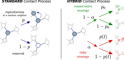
Figure 1: Left: Sketch of the standard contact process dynamics: each occupied node (individual) in the lattice either (i) produces an offspring with probability $p$ at a random neighboring site (provided it is empty) or (ii) is removed from the lattice with complementary probability $1-p$. Right: Contact process with hybrid dynamics: at each time step, every individual chooses between the conservative (with probability $1-\alpha$) and the risky (with probability $\alpha$) spreading strategy. The conservative dynamics is characterized by a constant, relatively low spreading probability $p_{0}$, while the risky one depends on a stochastic variable $p(t)$, common to all particles in the system.

Individuals can hedge their bets by randomly picking either of the two competing strategies at each time step. This choice is controlled by the “risk parameter” $\alpha$: at each time step, each individual independently adopts the risky strategy with probability $\alpha$ or the conservative one with probability $1-\alpha$ . In the language of game theory, $\alpha=0$ and $\alpha=1$ correspond to “pure strategies” and the range $0<\alpha<1$ corresponds to a set of hybrid strategies. In what follows, we assume that all individuals in the community are characterized by the same value of the risk parameter $\alpha$; variations in which $\alpha$ is individual-dependent are left for a future work. Key observables are the stationary density of individuals, $\rho$, the averaged (exponential) growth rate, $G$, and the mean extinction time of small populations, $\tau$ (see below).

III Theoretical insights

In game theory, it is known that a hybrid plan consisting in the alternation of two distinct pure strategies can outperform both of them (see, e.g., Kelly (1956); Harmer and Abbott (1999); Jansen and Yoshimura (1998); Williams and Hastings (2011)), constituting an example of Parrondo’s paradox. This effect plays an important role for our aims in what follows. In this section, we discuss a simplified one-variable equation aimed at capturing the gist of our model.

In particular, the simplifying assumptions we make here are as follows: (i) We consider a mean-field limit in which spatial fluctuations are neglected. (ii) We neglect nonlinear saturation terms; this is a valid approximation only for low densities. (iii) We consider a continuous time limit, as usually done to analyze the physics of the CP and other particle systems Gardiner (1985); Marro and Dickman (2005); Henkel et al. (2008) (a discrete-time calculation is presented in Appendix A to prove the robustness of our conclusions against this assumption). In the continuous-time limit, we consider the growth rate $p(t)=\bar{p}+\sigma\xi(t)$, where $\bar{p}$ and $\sigma$ are constants –the mean and amplitude of the stochastic risky strategy $p(t)$, respectively–, and where $\xi(t)$ is a Gaussian noise with $\langle\xi(t)\rangle=0$ and $\langle\xi(t)\xi(t^{\prime})\rangle=\delta(t-t^{\prime})$ [observe that even if we maintain the same notation as above, $p(t)$ and $p_{0}$ need to be interpreted as transition rates in the continuous-time approach]. The choice of a Gaussian probability distribution function for $p(t)$ enables us to obtain analytical calculations, but it has some “technical” drawbacks. In particular, being an unbounded distribution, $p(t)$ can take negative values; thus, in order to avoid interpretation problems, we need to restrict ourselves to the case $0\ll\bar{p}-\sigma$ and $\bar{p}+\sigma\ll 1$, where these effects should be negligible. In any case, even if specific details may depend on this choice, the general results and conclusions presented in what follows are robust against changes in this probability. This is explicitly illustrated in Appendix A for the case of uniform bounded distributions.

Under these assumptions, the density of individuals $\rho(t)$ obeys the following rate equation:

$$\dot{\rho}(t) =\alpha\left[p(t)\rho\left(1-\rho\right)-\left(1-p(t)\right)\rho\right]$$ (1)

$$+(1-\alpha)\left[p_{0}\rho\left(1-\rho\right)-\left(1-p_{0}\right)\rho\right].$$

Defining the average spreading rate,

$$p_{\mathrm{av}}(\alpha)=\alpha\bar{p}+(1-\alpha)p_{0},$$ (2)

Eq. (1) becomes

$$\dot{\rho}(t)=\left(2p_{\mathrm{av}}(\alpha)-1\right)\rho-p_{\mathrm{av}}(\alpha)\rho^{2}+2\alpha\sigma\rho\left(1-\frac{\rho}{2}\right)\xi(t),$$ (3)

which, owing to the stochastic nature of $p(t)$, is a Langevin equation, to be interpreted in the Itô sense. Up to leading linear order, we have the approximation

$$\dot{\rho}\approx\left(2p_{\mathrm{av}}(\alpha)-1\right)\rho+2\sigma\alpha\rho\xi(t),$$ (4)

valid for $\rho\ll 1$. Now changing variables (using Itô calculus) to $y=\log(\rho)$ and averaging over realizations $\langle\cdot\rangle$, eq. (4) becomes

$$\frac{d}{dt}\langle\log\rho\rangle=G(\alpha),$$ (5)

where the sign of the exponential growth rate,

$$G(\alpha)=-2\sigma^{2}\alpha^{2}+2p_{\mathrm{av}}(\alpha)-1,$$ (6)

determines whether the population tends to shrink or [owing to the absence of the nonlinear saturation terms in this approximation, Eq. (4)] to grow unboundedly. These two regimes are separated by a critical point at which $G(\alpha)=0$.

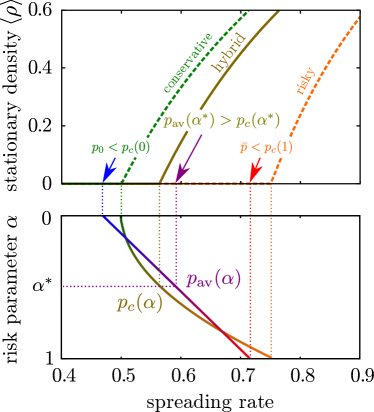
Figure 2: Top: Stationary density, computed via numerical integration of Eq. (3), for three types of strategies –conservative ($\alpha=0$), risky ($\alpha=1$), and a particular hybrid strategy ($0<\alpha^{*}<1$)– as a function of the spreading probability, $p_{0}$ in the conservative case and $\bar{p}$ in the risky and hybrid cases. Critical points for the pure strategies can be obtained analytically: $p_{c}(\alpha=0)=1/2$ and $p_{c}(\alpha=1)=1/2+\sigma^{2}$. Critical points for hybrid strategies lie between these two values. The lestmost (blue) and rightmost (red) arrows indicate a specific choice made for the two pure strategies, $\alpha=0$ and $\alpha=1$, respectively ($p_{0}=0.47$ and $\bar{p}=0.72$, with $\sigma^{2}=0.25$). Note that both of them are equally subcritical. The middle (purple) arrow marks the average spreading rate for a specific hybrid strategy (with $\alpha=\alpha^{*}$). Bottom: Two lines are plotted as a function of $\alpha$: the effective value of the spreading rate $p_{\mathrm{av}}(\alpha)$ and the location of the critical point, $p_{c}(\alpha)$. The first one interpolates linearly between our two pure-strategy choices (arrows) for $p_{0}$ and $\bar{p}$ in the pure cases (as indicated by the blue-red color gradient). On the other hand, the second line is a quadratic interpolation between the two pure-strategy critical points (as indicated by the green-orange gradient). As the two lines intersect each other, there exists a range of values of $\alpha$ for which $p_{\mathrm{av}}(\alpha)>p_{c}(\alpha)$ (supercritical) and others for which $p_{\mathrm{av}}(\alpha)<p_{c}(\alpha)$ (subcritical). In particular, for intermediate values of $\alpha$, such as the marked $\alpha^{*}=0.5$, the stochastic alternation of two subcritical strategies results in a supercritical one.

Keeping fixed all parameters but $\alpha$, we define the optimal strategy $\alpha^{*}\in[0,1]$ as the one maximizing $G(\alpha)$. This can be either a pure or a hybrid strategy, depending on parameter values. In particular, $\alpha^{*}=0$ for $\bar{p}<p_{0}$, $\alpha^{*}=1$ for $\bar{p}>p_{0}+2\sigma^{2}$, and $\alpha^{*}={(\bar{p}-p_{0})}/{2\sigma^{2}}$ for intermediate values of $\bar{p}$. Observe that the critical point is obtained for $p_{c}(\alpha)=\frac{1}{2}+\sigma^{2}\alpha^{2}$, i.e., the $\alpha$-dependent critical point interpolates quadratically between the critical points of the pure strategies, $p_{c}(0)=\frac{1}{2}$ and $p_{c}(1)=\frac{1}{2}+\sigma^{2}$. On the other hand, the average spreading rate $p_{\mathrm{av}}(\alpha)$ [Eq. (2)] is a linear-in-$\alpha$ interpolation between the two limiting pure values.

Figure 2 (top) shows the stationary density [obtained via numerical integration of Eq. (3)] for the conservative, the risky, and an intermediate hybrid strategy. The critical points at which the nontrivial steady states emerge coincide with the analytical predictions we have just made. As explained in the caption to Fig. 2, the different functional dependences for $p_{\mathrm{av}}(\alpha)$ and $p_{c}(\alpha)$ –linear and quadratic in $\alpha$, respectively– enable the two curves to intersect each other, and thus, for intermediate values of $\alpha$ it is possible to have $p_{\mathrm{av}}(\alpha)>p_{c}(\alpha)$, i.e., a supercritical dynamics, even in the case (illustrated in Fig. 2) in which both pure strategies, $p_{0}$ and $\bar{p}$, are subcritical. Similarly, when the two pure strategies are active/supercritical, the same argument shows that a much higher stationary density can be achieved by hybrid strategies.

This graphical representation –which we believe is new in the literature– allows us to understand in a relatively simple and compact way the essence of Parrondo’s paradox. In what follows, we consider different types of pure strategies, either absorbing/subcritical or active/supercritical, and quantify the gain induced by bet-hedging in different settings, including fully connected (FC) networks (where the above mean-field approach should hold) and spatially explicit low-dimensional systems (where mean-field conclusions might break down).

IV Computational results

The calculation in the previous section provides valuable insight into why hybrid strategies can be important, but it has some important limitations. It is a mean-field calculation, thus neglecting spatial structure. Moreover, Eq. (4) includes only linear terms, and thus it can only describe exponential growth starting from low density rather than the steady-state behavior of the nonlinear dynamics. To go beyond these limitations, here we perform direct Monte Carlo simulations of the discrete model defined in Sec. II in large FC networks, and later we compare them with similar simulations in one-dimensional (1D) two-dimensional (2D) and three-dimensional (3D) lattices.

We implemented the CP dynamics using either synchronous/parallel or asynchronous/sequential types of updatings. Here, we mostly focus on the synchronous case. In Appendix B, we show that asynchronous updating leads to qualitatively similar results, even if quantitative differences emerge.

Simulations are initialized with a fully occupied configuration; then the dynamics proceeds as follows: (i) At every step, a new value of $p(t)$ is drawn from some probability distribution in $[0,1]$; in most of this paper we use a truncated Gaussian $N(\bar{p},\sigma^{2})$ ($\bar{p}$ and $\sigma^{2}$ are the mean and variance, respectively, of the nontruncated distribution) in which we fix possible values $p(t)<0$ to $p(t)=0$ and values $p(t)>1$ to $1$. This particular choice may seem arbitrary, but we have verified that all the forthcoming conclusions are robust and remain valid for, e.g., uniform distributions. (ii) The network/lattice is updated synchronously; with probabilities $\alpha$ and $1-\alpha$, each individual selects the risky or the conservative strategy respectively. (iii) Each individual either dies or reproduces with the corresponding probabilities; all dying individuals are removed from the system and afterward offspring are placed at random neighbors of their corresponding parents, keeping the constraint of a maximum occupancy of one individual per site (i.e., offspring trying to occupy an already full site are simply removed). Finally, (iv) time is incremented in one unit and the process is iterated until a stationary state has been reached and steady-state measurements (of, e.g., $\rho$) are performed.

We begin by verifying the possibility of obtaining an active phase by combining two strategies, each of them leading to an absorbing/subcritical phase. To this aim, we fix the parameters $(p_{0},\bar{p},\sigma)$ to poise the respective pure strategies ($\alpha=0$ or $\alpha=1$) in the absorbing phase and study the behavior of hybrid strategies at intermediate values of $\alpha$. To determine whether or not a strategy leads to an active phase, we measure the mean extinction time, $\tau$, as a function of the system size $N$. Observe that, owing to fluctuations, any finite system is condemned to end up in the absorbing state. However, its mean lifetime increases exponentially with $N$, $\tau\sim\exp(N)$ in the active phase Gardiner (1985), making the system stable in the large-$N$ limit. Note that, in the presence of fluctuating parameters, $\tau(N)$ can also scale as a power-law in the active phase Vazquez et al. (2011). On the other hand, a slow logarithmic increase, $\tau\sim\log(N)$, is expected in the absorbing phase Gardiner (1985); Vazquez et al. (2011). As shown in Fig. 3 for different values of $\alpha$ and for different spatial dimensions, $\tau$ grows logarithmically with $N$ for the two pure strategies ($\alpha=0,1$), as corresponds to both of them being absorbing, while it increases exponentially for an intermediate range of hybrid strategies, which depends upon the systems dimensionality. We therefore conclude that in the CP the stochastic alternation of two absorbing dynamics can lead to an active one, in agreement with the linear-approximation above.

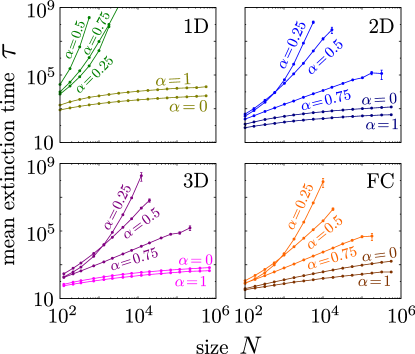
Figure 3: Mean extinction times as a function of system size $N$ for different strategies $\alpha$ and spatial dimensions. For our parameter choice, the two pure strategies, $\alpha=0,1$, have a logarithmic dependency (characteristic of subcritical behavior Vazquez et al. (2011)), while a range of hybrid strategies exhibits an exponential or power-law increase typical of active phases Vazquez et al. (2011). Parameter values $(p_{0},\bar{p},\sigma)$: 1D, $(0.71,0.80,0.20)$; 2D, $(0.58,0.71,0.29)$; 3D, $(0.54,0.69,0.30)$, and fully connected (FC), $(0.499,0.67,0.33)$. Most error-bars are smaller than the symbol sizes.

Some remarks are in order. The advantageous consequences of bet-hedging are not limited to the mean-field case, which can be simply interpreted in terms of Eq. (3), but are important also in low-dimensional systems where internal fluctuations play a key role. Observe also that, as the phase boundaries depend on dimensionality, different parameters are chosen for different panels in Fig. 3. We discuss later a way to compare more clearly the strength of the effect as the system dimensionality is changed. Finally, we have made no attempt here to accurately determine the values of $\alpha$ delimiting the active phase for each dimension, but have just confirmed the stabilizing effect of hybrid strategies.

The goal now is to quantitatively analyze how the benefits of bet-hedging depend on the level of stochasticity, both external (environmental) and intrinsic (demographic).

IV.1 Environmental/external noise

First, we study the dependence on environmental variability $\sigma^{2}$. To ease comparison, for each value of $\sigma^{2}$, we fix the two pure strategies to have the same steady-state density, $\langle\rho(\alpha=0)\rangle=\langle\rho(\alpha=1)\rangle=0.3$, by an appropriate choice of the only remaining free parameters, $p_{0}$ and $\bar{p}$, respectively. Observe that, at variance with the previous section, here the pure strategies are taken to be “equally” active (same steady-state density), but we could have also taken them to be equally absorbing (same extinction time). The reason for this choice is that it allows for a much faster and easier computational implementation. We then analyze how the steady-state averaged density $\rho$ depends on $\alpha$ for different values of $\sigma^{2}$. Figure 4(a) clearly illustrates that, in the case of FC (mean-field) lattices, more variable environments allow bet-hedging strategies to achieve much higher stationary densities. The same trend holds for low-dimensional lattices (not shown): the larger the external noise, the more benefits a community can derive from conveniently exploiting bet-hedging.

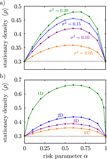
Figure 4: (a) Effect of the external-noise variability ($\sigma^{2}$) on the stationary density for different bet-hedging strategies. Curves are results of Monte Carlo simulations of the fully-connected (FC) CP with bet-hedging. As $\sigma^{2}$ is increased, the optimal strategy induces higher stationary densities, even if the pure strategies $\alpha=0,1$ lead to the same density, $\langle\rho(\alpha=0,1)\rangle=0.3$. Parameter values are $N=10^{4}$, $p_{0}=0.567$. $(\bar{p},\sigma^{2})$ are $(0.628,0.05)$, $(0.699,0.10)$, $(0.765,0.15)$ and $(0.825,0.20)$ in the different curves. (b) Effect of dimensionality at fixed $\sigma^{2}$. The net benefit of bet-hedging is much enhanced at lower-dimensions. Parameters: $\langle\rho(\alpha=0,1)\rangle=0.3$, $\sigma^{2}=0.05$, $N=10^{4}$ for 1D, 2D and FC, $N=10648$ for 3D, and $(p_{0},\bar{p})$ are 1D:$(0.722,0.847)$, 2D:$(0.618,0.704)$, 3D:$(0.594,0.665)$ and FC:$(0.567,0.628)$. Error-bars are smaller than symbol sizes in all cases.

This observation is consistent with the linear analysis embodied in Eq.(4). Using the definition of $G(\alpha)$ and keeping the environmental variance $\sigma^{2}$ as a control parameter, $p_{0}$ and $\bar{p}$ can be fixed by imposing identical growth rates for the pure strategies, $G(0)=G(1)\equiv G_{0,1}$. Under this constraint, the maximum possible growing rate is

$$\max(G)=G(\alpha=1/2)=G_{0,1}+\frac{\sigma^{2}}{2},$$ (7)

predicting a linear increase in the optimal G with $\sigma^{2}$.

As a final remark, observe that, although the two pure strategies have been set to be equivalent (in the sense that both lead to the same stationary density), the optimal strategy $\alpha^{*}$ in Fig. 4(a) (maximizing $\langle\rho\rangle$) tends to be slightly larger than that provided by the approximate analytical prediction $\alpha^{*}=1/2$ (maximizing $G$). We have checked that this “favoring” of the risky strategy strongly depends on the details of the implementation, as we have not observed it with asynchronous updating in the dynamics (see Appendix B). So far, we have not attempted to determine the optimal strategy $\alpha^{*}$ for each case, but just to confirm the gain enhancement of bet-hedging in the presence of larger fluctuations.

IV.2 Dimensionality and demographic/intrinsic noise

A main feature of low-dimensional models in statistical mechanics is that intrinsic fluctuations (or demographic stochasticity, in the language of population dynamics) play a more dramatic role than they do in high dimensions Binney et al. (1993), where they can be safely neglected in mean-field-like approximations. We assume –and then explicitly verify– that smaller spatial dimensions effectively correspond to larger levels of demographic noise.

We now explore the effect of dimensionality on bet-hedging; the spatial dimension of the systems is varied while keeping a fixed external noise variance $\sigma^{2}$. As above, to ease comparison, we choose pure strategies for each dimension so that $\langle\rho(0)\rangle=\langle\rho(1)\rangle=0.3$ (i.e., both pure strategies are equally active) and measure computationally $\langle\rho\rangle$ as a function of $\alpha$ for hybrid strategies in each dimension.

Figure 4(b) clearly illustrates that the benefits of bet-hedging are much enhanced as the system dimensionality is decreased, allowing for much higher densities. In particular, 1D systems can accommodate twice as much density as FC (infinite-dimensional) lattices.

A simple mathematical argument allows us to qualitatively –even if not quantitatively– understand this finding. Demographic noise is the key ingredient, missing in the mean-field limit. Therefore, we generalize Eq. (4) to include a demographic-noise term of tunable amplitude $\gamma$ Gardiner (1985); Muñoz (1998) as well as the above-neglected leading nonlinear term

$$\dot{\rho}(t)\approx\left(2p_{\mathrm{av}}(\alpha)-1\right)\rho-p_{\mathrm{av}}(\alpha)\rho^{2}+2\alpha\sigma\rho\xi(t)+\gamma\sqrt{\rho}\eta(t),$$ (8)

where $\eta(t)$ is a Gaussian white noise. As usual, the square-root factor multiplying the noise amplitude of demographic fluctuations is a direct consequence of the central limit theorem, which, in particular, imposes that fluctuations disappear in the absence of activity ($\rho=0$) Gardiner (1985).

Equivalently to Eq. (8), we can write down the Fokker-Planck equation for the probability distribution $P(\rho,t)$ Gardiner (1985). To work in the quasi-stationary approximation Gardiner (1985); Dickman and Vidigal (2002); Muñoz (1998) (i.e., to avoid technical problems stemming from the existence of an absorbing state at $\rho=0$), we include a small and constant drift $\varepsilon$, which is a constant added on the right hand side of Eq. (8), giving:

$$\partial_{t}P(\rho,t) = -\frac{\partial}{\partial\rho}\left[\left(\varepsilon+\left(2p_{\mathrm{av}}(\alpha)-1\right)\rho-p_{\mathrm{av}}(\alpha)\rho^{2}\right)P(\rho,t)\right]$$ (9)

$$+\frac{1}{2}\frac{\partial^{2}}{\partial\rho^{2}}\left[(\beta^{2}\rho+\gamma^{2})\rho P(\rho,t)\right],$$

where, for convenience, we have introduced $\beta=2\alpha\sigma$. The associated stationary probability distribution function then reads:

$$P_{\mathrm{st}}(\rho)=\left\{\begin{array}[]{l}C_{1}\,\rho^{\frac{2\varepsilon}{\gamma^{2}}-1}\exp{\left(\frac{2(2p_{\mathrm{av}}-1)\rho-p_{\mathrm{av}}\rho^{2}}{\gamma^{2}}\right)},\quad\beta=0\\ \\ C_{2}\,\rho^{\frac{2\varepsilon}{\gamma^{2}}}\left(\gamma^{2}+\beta^{2}\rho\right)^{\frac{2(2p_{\mathrm{av}}-1)}{\beta^{2}}+\frac{2p_{\mathrm{av}}\gamma^{2}}{\beta^{4}}-\frac{2\varepsilon}{\gamma^{2}}-1}\times\\ \qquad\exp{\left(-\frac{2p_{\mathrm{av}}\rho}{\beta^{2}}\right)},\quad\beta>0,\end{array}\right.$$ (10)

where $C_{1}$ and $C_{2}$ are normalization constants. From this equation we can compute the averaged quasi-stationary density

$$\langle\rho\rangle=\int_{0^{+}}^{\infty}d\rho\,\rho\,P_{\mathrm{st}}(\rho)$$ (11)

as a function of parameter values.

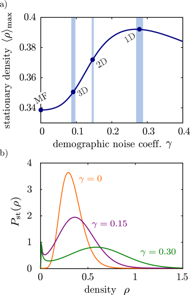
Figure 5: (a) Stationary density of the optimal hybrid strategy as a function of the demographic noise amplitude $\gamma$: each point was computed using the value of $\gamma$ inferred from Eq. (10), for a different spatial dimension ($1$, $2$, and $3$), and $\gamma=0$ for the mean-field case. Parameters $p_{0}$, $\bar{p}$, and $\sigma$ are the same as in Fig. 4(b) and $\gamma$ is tuned to produce $\langle\rho(\alpha=0)\rangle=\langle\rho(\alpha=1)\rangle=0.3$. The inferred $\gamma$ changes slightly for $\alpha=0$ and $\alpha=1$ as reflected in the error bars (shaded region). These results confirm that the effective noise amplitude $\gamma$ increases as the system dimensionality decreases and that the benefits of bet-hedging are enhanced by demographic noise. However, the curve becomes nonmonotonous for larger values of $\gamma$. (b) Density distributions in the optimal strategy $\alpha^{*}$ for different demographic noise amplitudes $\gamma$: We represent the quasistationary solution of Eq. (10) ($\varepsilon=10^{-3}$). The calculus fails for higher values of $\gamma$, as the probability of decay into the absorbing state (emerging peak at $\rho=0$) becomes non-negligible. The functional dependence of $\langle\rho\rangle_{\mathrm{max}}(\gamma)$ does not change qualitatively for other choices of this parameter, such as $\varepsilon=10^{-2},10^{-3}$ or $10^{-4}$.

The effective dimension-dependent value of $\gamma$ can now be inferred from the condition that –fixing the remaining parameters (i.e., $p_{0}$, $\bar{p}$, and $\sigma^{2}$) as in each of the spatially explicit simulations [see caption of Fig. 4b]– the quasi-stationary density in Eq. (11) satisfies $\langle\rho(\alpha=0)\rangle=\langle\rho(\alpha=1)\rangle=0.3$. The resulting values of $\gamma$ are $\gamma=0.09,0.15$, and $0.28$, for dimensions $3$, $2$, and $1$, respectively (each value is the average of two very close results obtained for the two pure strategies), confirming that, as expected, $\gamma$ –effectively representing the amplitude of demographic noise– increases upon lowering the spatial dimension.

Having determined, for each dimension, the level of demographic fluctuations $\gamma$, we now use Eqs. (10) and (11) to compute the maximum density as a function of $\alpha$. Results are shown in Fig. 5, which reveals that the benefits of bet-hedging are enhanced for larger demographic noises and, thus, for lower spatial dimensions.

We remark that this phenomenological single-variable theory only provides a qualitative explanation of the phenomenon and does not quantitatively reproduce the actual stationary densities in Fig. 4(b). Observe also that for very high noise amplitudes the curve in Fig. 5 veers down, while this effect is not seen when reducing the system dimensionality. A more rigorous analytical approach to this problem –including the explicitly spatial dependence in Eq. (8)– is a challenging task, beyond the scope of the present work.

IV.3 Time-correlated environments

In the model we have discussed, the timescale of environmental changes is the same as the generation times cale. However, real biological populations have to cope with environmental conditions varying on time scales possibly longer Schwager et al. (2006) than the individual generation time. To address this important generalization, we checked how our main results change upon varying the temporal correlation of the state of the environment. In particular, we simply described $p(t)$ as an Ornstein-Uhlenbeck process (see, e.g., Gardiner (1985)) of average $\bar{p}$ and variance $\sigma^{2}$ and study the effect of varying its correlation time.

Detailed results of this study are summarized in Appendix C. Our main conclusion, i.e., that the benefits of bet-hedging strategies are enhanced in lower-dimensional systems, remains unaltered. In addition, considering an environment correlated over a few generations enhances the advantage of bet-hedging in all dimensions, although this effect is significantly stronger in low dimensions. Finally, the optimal strategy becomes more conservative for environments characterized by a very long correlation time. These results can be intuitively understood by thinking that, if the environment is persistently unfavorable for a long time, the extinction risk is very high, and bet-hedging strategies become more crucial for survival. A much more detailed analytical characterization of bet-hedging dynamics under correlated environments is left for a future study.

V Conclusions

Summarizing, our main finding is that the relative benefit of developing bet-hedging strategies is strongly enhanced in highly fluctuating low-dimensional systems, where both internal and external sources of variability greatly foster dynamical fluctuations, leading to a strong departure from mean-field behavior. Given that these conditions are often met by biological populations –as for instance, in bacterial colonies competing at the front of a range expansion in noisy environments Ben-Jacob et al. (1994); Korolev et al. (2010); Weber et al. (2014)– our results support the importance of bet-hedging in nature. This being said, of course, more realistic models –including some realistic ingredients such as, for example, the possibility of “dormant” states and not just birth and death processes– would be required to approach viral or bacterial communities and their bet-hedging more closely.

The kind of trade-off considered in this paper, between a stable and a fluctuating resource, is possibly the simplest example of bet-hedging, both biologically relevant and natural to understand using tools of nonequilibrium statistical physics. However, we conjecture that the increased strength of bet-hedging in low dimensionality is a general phenomenon, present in other recently studied examples of trade-offs, for example, between reproduction and motility Reiter et al. (2014); Pigolotti and Benzi (2014) and in pairwise games Rulands et al. (2014).

Our preliminary results presented in Appendix C show that the effect described in this paper is still present in correlated environments. However, for very long correlation times, bet-hedging strategies are disfavored compared to short-correlated environments, but they always provide an advantage with respect to pure strategies. In view of these preliminary results, it will be of interest to investigate from a general perspective and in more depth the influence of environmental-noise temporal autocorrelations on bet-hedging, as well as the difference between exploiting bet-hedging individually and exploiting it at a community level. We believe that this work will provide a physical framework to answer these and similar challenging questions which might be of interest in biology and ecology.

Appendix A Uniformly distributed environment

In this Appendix we study the case in which the spreading probability for the risky strategy, $p(t)$, is bounded and uniformly distributed in the range $[\bar{p}-\delta,\bar{p}+\delta]$, where the parameter $\delta$ encapsulates the level of environmental variability. In particular, to avoid negative values, we take $\delta<\bar{p}$ and $\delta<1-\bar{p}$. This type of distribution allows for analytical treatment using a discrete-time approach, which is common in the study of game theory Kelly (1956). To proceed, we take the linearized rate equation derived in the text, Eq. (4), and write it in a discrete-time form (using one-unit time steps) and replace $p(t)$ with its explicit form for the uniform distribution,

$$\rho(t)=2p_{\mathrm{av}}(\alpha)\rho(t-1)+2\alpha\delta\rho(t-1)u(t-1),$$ (12)

where $u(t)$ is a uniformly distributed variable in the range $[-1,1]$, for any integer $t\geq 0$.

Assuming an initial density $\rho(0)$ and discretizing the range of values of $u$, $u=(u_{1},...,u_{U})$, the previous equation becomes

$$\rho(t)=\prod_{i=1}^{U}\left[2p_{\mathrm{av}}(\alpha)+2\alpha\delta u_{i}\right]^{n_{i}}\rho(0),$$ (13)

where $n_{i}$ is the number of times that a value $u_{i}$ is obtained, and therefore, $\sum_{i}n_{i}=t$. The exponential growth rate is derived from its discrete form, $G=\lim_{t\rightarrow\infty}\frac{1}{t}\log\frac{\rho(t)}{\rho(0)}$ Kelly (1956),

$$G(\alpha)=\sum_{i=1}^{U}\frac{n_{i}}{t}\log\left[2p_{\mathrm{av}}(\alpha)+2\alpha\delta u_{i}\right],$$ (14)

which in the continuum limit becomes

$$G(\alpha) = \int_{-1}^{1}du\frac{1}{2\delta}\log\left[2p_{\mathrm{av}}(\alpha)+2\alpha\delta u\right]=\log(2)-1+$$ (15)

$$\frac{1}{2\delta\alpha}\log{\frac{\left(p_{\mathrm{av}}(\alpha)+\alpha\delta\right)^{p_{\mathrm{av}}(\alpha)+\alpha\delta}}{\left(p_{\mathrm{av}}(\alpha)-\alpha\delta\right)^{p_{\mathrm{av}}(\alpha)-\alpha\delta}}},$$

for any $\alpha\in(0,1]$, and $G(0)=\log\left(2p_{0}\right)$ for $\alpha=0$.

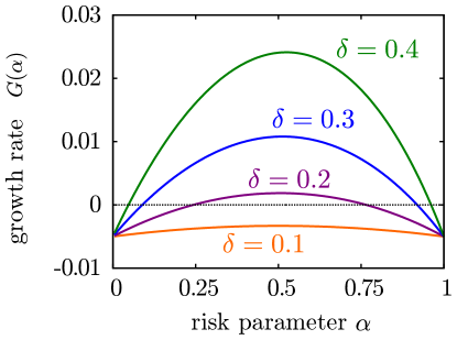
Figure 6: Exponential growth rate $G$ as a function of the risk parameter $\alpha$ as given by Eq. (15) for uniformly distributed environments: $p(t)=\bar{p}+\delta u(t)$, where $\bar{p}$ and $\delta$ are constants and $u(t)$ is a uniform noise distributed in $[-1,1]$. Different curves correspond to different values of the parameter $\delta$; in all cases the corresponding pure strategies have been tuned to give $G(\alpha=0)=G(\alpha=1)=-0.005$ in the absorbing/subcritical phase. The optimal strategy is always a hybrid one, very close to $\alpha^{*}=0.5$. In particular, for $\delta\gtrsim 0.15$, $G(\alpha^{*})>0$, allowing for active/supercritical dynamics. Furthermore, the maximum growth rate for this strategy increases with the amplitude of the environmental noise. Parameter values: $p_{0}=0.498$ fixed in all cases, and $(\bar{p},\delta)=(0.501,0.1),(0.511,0.2),(0.528,0.3)$ and $(0.553,0.4)$. Note that $\delta<\bar{p}$ and $\delta<1-\bar{p}$ in all cases.

Figure 6 shows the solution $G$ as a function of $\alpha$ [Eq. (15)] for different choices of the environmental variability $\delta$. In this example, we have tuned the parameters $p_{0}$ and $\bar{p}$ to be equally subcritical, i.e., $G(0)=G(1)<0$, but similar curves can be obtained if $G(0)=G(1)>0$. We see that (i) the optimal strategy, in the sense of having a maximal $G$, always lies at intermediate values of $\alpha$; (ii) the growth rate for such optimal strategy increases with the amplitude of fluctuations $\delta$; and (iii) for sufficiently large values of $\delta$, a combination of two subcritical strategies gives rise to a supercritical one, as $G(\alpha^{*})>0$ for $\delta\gtrsim 0.15$. Moreover, we have tested these results in Monte Carlo simulations, as well as with different lattice dimensions, obtaining plots similar to Fig. 4 and Fig. 7. Summarizing, in the case in which $p(t)$ is uniformly distributed, the same conclusion obtained for Gaussian distributions holds: the benefits of bet-hedging are stronger in the presence of both extrinsic and intrinsic fluctuations.

Appendix B Model with asynchronous updating

In this Appendix, we verify the robustness of our results when an asynchronous-updating version of the CP Marro and Dickman (2005) is implemented. At each time step, one of the existing $N_{\mathrm{act}}(t)$ active particles is randomly selected; with probability $\alpha$, the particle chooses the risky strategy or, with complementary probability $1-\alpha$, the conservative one. As above, in the first case, it reproduces with probability $p(t)$ or dies with probability $1-p(t)$, where $p(t)$ changes with the environment, while for the conservative strategy it reproduces with probability $p_{0}$ or dies with probability $1-p_{0}$. Time is incremented in $1/N_{\mathrm{act}}(t)$. After all particles in the network have been updated once on average (i.e. after time increases in one unit) another value of $p(t)$ is drawn from a Gaussian distribution $N(\bar{p},\sigma^{2})$.

With this implementation, as in Fig. 4, we have again computed the curve $\langle\rho(\alpha)\rangle$ provided that $\langle\rho(0,1)\rangle=0.3$, for different values of the external noise variance $\sigma^{2}$ (in the FC network) and for different network dimensions (fixing $\sigma^{2}$). As illustrated in Fig. 7, the relative position of all curves is the same as for the case of synchronous updating: the benefits of bet-hedging are enhanced as the noise amplitude is increased. However, quantitatively, the enhancement is smaller than in the synchronous case, discussed in the text.

As a final remark, observe that one could have naively expected that fluctuations derived from the sequential updating might contribute to an enhancement of the density for such hybrid strategies. This difference stems from the fact that in the sequential implementation of the model, not all individuals are necessarily updated at every single Monte Carlo step; thus the stochasticity introduced by this type of updating may save populations from extinctions in very unfavorable environments. This implies that the community does not rely as strongly on bet-hedging to perdure.

Figure 7: Effect (a) external-noise variability ($\sigma^{2}$) in the fully connected (FC) network and (b) dimensionality at fixed $\sigma^{2}$ on the stationary density for different bet-hedging strategies with asynchronous updating. Curves are results of Monte Carlo simulations of the CP with bet-hedging. Qualitatively, the same conclusions are obtained as with the parallel updating. However, the benefits of bet-hedging strategies become lower in this second implementation, especially for the FC network. Parameter values are as follows. (a) $N=10^{4}$; $p_{0}=0.588$; and $(\bar{p},\sigma^{2})$ of $(0.597,0.05)$, $(0.610,0.10)$, $(0.624,0.15)$ and $(0.637,0.20)$ in the different curves. (b): $\sigma^{2}=0.05$; $N=10^{4}$ for 1D, 2D, and FC, $N=10648$ for 3D, and $(p_{0},\bar{p})$ are 1D:$(0.770,0.831)$, 2D:$(0.655,0.681)$, 3D:$(0.626,0.642)$ and FC:$(0.588,0.597)$. Most error-bars are smaller than symbol sizes.

Appendix C Effect of temporal correlations

A simple way to introduce temporal autocorrelations in the environment is to take $p(t)$ to follow a Ornstein-Uhlenbeck process Gardiner (1985), i.e., a Brownian particle moving in a parabolic potential. Mathematically, this process obeys Gardiner (1985)

$$\dot{p}=\theta(\bar{p}-p)+\sqrt{2\theta}\sigma\xi(t),$$ (16)

where $\bar{p}$ and $\sigma$ represent, as before, the mean and variance of $p(t)$, respectively. With this choice, $p(t)$ is Gaussian distributed, $N(\bar{p},\sigma^{2})$. The new parameter $\theta$ controls the temporal autocorrelations, as $\langle\left(p(t)-\bar{p}\right)\left(p(t^{\prime})-\bar{p}\right)\rangle=\sigma^{2}e^{-\theta|t-t^{\prime}|}$; consequently, $\theta\rightarrow 0$ and $\theta\rightarrow\infty$ represent the extreme cases of immutable (completely correlated) and delta-correlated environments, respectively.

Equation (16) can be integrated exactly, allowing for a recursive generation of values at successive time steps San Miguel and Toral (2000),

$$p(t+1)=\bar{p}(1-e^{-\theta})+p(t)e^{-\theta}+\sigma\sqrt{1-e^{-2\theta}}N(0,1),$$ (17)

where $N(0,1)$ is a zero-mean unit-variance Gaussian random number.

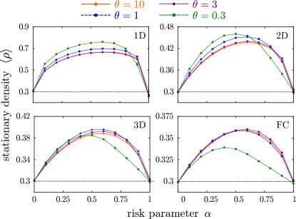
Figure 8: Stationary density as a function of the risk parameter for different lattice topologies in temporal-correlated environments: the spreading probability of the risky strategy, $p(t)$ now obeys an Ornstein-Uhlenbeck process with mean $\bar{p}$, variance $\sigma^{2}$, and exponential temporal correlations with a characteristic time ${\theta}^{-1}$. The benefits of the hybrid strategies in the stationary density become enhanced for intermediate values of $\theta$. This result is much intensified in lower dimensions, while it is imperceptible for the 3D and FC networks. Parameters: $\sigma^{2}=0.05$; $(\bar{p},\theta)$ in 1D: $(10,0.848)$, $(3,0.849)$, $(1,0.876)$, $(0.3,0.944)$; 2D: $(10,0.704)$, $(3,0.706)$, $(1,0.719)$, $(0.3,0.745)$; 3D: $(10,0.665)$, $(3,0.667)$, $(1,0.674)$, $(0.3,0.681)$ and FC: $(10,0.628)$, $(3,0.629)$, $(1,0.631)$, $(0.3,0.624)$; $p_{0}$ and $N$, taken as in Fig. 4(b).

Fixing the environmental variance $\sigma^{2}$, we numerically study the effect of temporal correlations on bet-hedging for different values of $\theta$ in every dimension. Following the same strategy as above, we tune the parameters $p_{0}$ and $\bar{p}$ for each temporal autocorrelation $\theta$ to fix the stationary density at $\langle\rho(\alpha=0,1)\rangle$, and measure $\langle\rho(\alpha)\rangle$. Results are summarized in Fig. 8. Some remarks are in order. (i) The optimal strategy is always a hybrid strategy between $\alpha=0$ and $\alpha=1$. Additionally, curves coincide with those in Fig. 4(b) when $\theta$ is high ($\theta\sim 10$), as the external environment exhibits only short correlations. (ii) When $\theta$ decreases moderately, the stationary density at the optimal strategy becomes larger compared to the noncorrelated case. In other words, bet-hedging strategies are more efficient for temporally autocorrelated environments. This effect is stronger for lower dimensions, whereas it barely applies to higher dimensional lattices. (iii) When the autocorrelation is very large ($\theta<0.1$), the benefits of hybrid strategies are reduced compared to the noncorrelated case, but they always remain convenient with respect to pure strategies. However, we are not interested in this scenario, in which external conditions remain almost unchanged during extremely long periods of time, and thus it behaves, effectively as a constant-$p$ case. The inflection point in $\theta$ at which this effect appears varies for different dimensions. (iv) Finally, the optimal strategy becomes more conservative when temporal correlations are added to the environment, with a bias to $\alpha^{*}\rightarrow 0$ when $\theta$ decreases. It would be nice to have a more detailed analytical understanding of all this phenomenology, but we leave this challenging task for future work.