2.4cm2.4cm2cm2cm

QMUL-PH-14-27

We apply MHV diagrams to the derivation of the one-loop dilatation operator of ${\cal N}=4$ super Yang-Mills in the $SO(6)$ sector. We find that in this approach the calculation reduces to the evaluation of a single MHV diagram in dimensional regularisation. This provides the first application of MHV diagrams to an off-shell quantity. We also discuss other applications of the method and future directions.

1 Introduction

The study of $\mathcal{N}=4$ supersymmetric Yang-Mills (SYM) theory has led to the discovery of integrability in the planar limit, providing the tools to compute the anomalous dimensions of local operators for any value of the coupling. In an initially independent line of research into this theory, the study of its on-shell scattering amplitudes has uncovered a rich structure and simplified calculations dramatically. It is widely expected that the integrability of the planar anomalous dimension problem and the hidden structures and symmetries of scattering amplitudes are related in some interesting way. In this paper we take a first step towards unravelling this potential connection.

Specifically, our goal here is to apply a method originally devised for computing amplitudes known as MHV diagrams [1] to the derivation of the one-loop dilatation operator $\Gamma$ in the $SO(6)$ sector of ${\cal N}=4$ SYM, originally computed by Minahan and Zarembo (MZ) in [2]. It is known that MHV diagrams are obtained from a particular axial gauge choice, followed by a field redefinition [3, 4], hence the validity of the method not only applies to on-shell amplitudes, but also to off-shell quantities such as correlation functions. This paper provides the first application of the MHV diagram method to the computation of correlation functions.

There are several reasons to pursue an approach based on MHV diagrams. Firstly, it is interesting to consider the application of this method to the computation of fully off-shell quantities such as correlation functions. Secondly, in the MHV diagram method there is a natural way to regulate the divergences arising from loop integrations, namely dimensional regularisation, used in conjunction with the four-dimensional expressions for the vertices. In this respect, we recall that one-loop amplitudes were calculated with MHV diagrams in [5], where the infinite sequence of MHV amplitudes in ${\cal N}=4$ SYM was rederived. One-loop amplitudes in ${\cal N}=1$ SYM were subsequently computed in [6, 7], while in [8] the cut-constructible part of the infinite sequence of MHV amplitudes in pure Yang-Mills at one loop was presented. The ${\cal N}=1$ and ${\cal N}=0$ amplitudes have ultraviolet (UV) divergences (in addition to infrared ones), which are also regulated in dimensional regularisation. The two-point correlation function we compute in this paper also exhibits UV divergences, which we regulate in exactly the same way as in the case of amplitudes.

An additional motivation for our work is provided by the interesting recent papers [11, 12]. In particular, [11] successfully computed $\Gamma$ using ${\cal N}=4$ supersymmetric twistor actions [13, 14, 15]. It is known that such actions, in conjunction with a particular axial gauge choice, generate the MHV rules in twistor space [14], and the question naturally arises as to whether one could derive the dilatation operator directly using MHV diagrams in momentum space, without passing through twistor space. The answer to this question is positive, and furthermore we find that the calculation is very simple – it amounts to the evaluation of a single MHV diagram in dimensional regularisation, leading to a single UV-divergent integral, identical to that appearing in [2].

The rest of the paper is organised as follows. In the next section we briefly review the result of [2] for the integrable Hamiltonian describing the one-loop dilatation operator $\Gamma$ in the $SO(6)$ sector. In Section 3 we address the calculation of $\Gamma$ using MHV diagrams. We present our conclusions and suggestions for future research in Section 4.

2 The one-loop dilatation operator

The computation of the dilatation operator in the $SO(6)$ sector of the ${\cal N}=4$ SYM theory is equivalent to extracting the UV-divergent part of the two-point function $\left\langle{\cal O}(x_{1})\bar{\cal O}(x_{2})\right\rangle$, where ${\cal O}$ is a single-trace scalar operator, of the form

$${\cal O}_{A_{1}B_{1},A_{2}B_{2},\ldots,A_{L}B_{L}}(x)\ :=\ {\rm Tr}\big{(}\phi_{A_{1}B_{1}}(x)\cdots\phi_{A_{L}B_{L}}(x)\big{)}\ .$$ (2.1)

At one loop and in the planar limit, only nearest neighbour scalar fields can be connected by vertices. This simplifies the calculation to that of $\left\langle(\phi_{AB}\phi_{CD})(x_{1})(\phi_{A^{\prime}B^{\prime}}\phi_{C^{\prime}D^{\prime}})(x_{2})\right\rangle$. The expected flavour structure of this correlation function is

$$\left\langle(\phi_{AB}\phi_{CD})(x_{1})(\phi_{A^{\prime}B^{\prime}}\phi_{C^{\prime}D^{\prime}})(x_{2})\right\rangle\!=\!{\cal A}\,\epsilon_{ABCD}\epsilon_{A^{\prime}B^{\prime}C^{\prime}D^{\prime}}+{\cal B}\,\epsilon_{ABA^{\prime}B^{\prime}}\epsilon_{CDC^{\prime}D^{\prime}}+{\cal C}\,\epsilon_{ABC^{\prime}D^{\prime}}\epsilon_{A^{\prime}B^{\prime}CD}.$$

These three terms are usually referred to as trace, permutation and identity. We are only interested in computing the leading UV-divergent contributions to the coefficients ${\cal A}$, ${\cal B}$ and ${\cal C}$, which according to [2] are expected to be

$${\cal A}_{\rm UV}\ =\ {1\over 2}\,,\qquad{\cal B}_{\rm UV}\ =\ -1\,,\qquad{\cal C}_{\rm UV}\ =\ 1\ .$$ (2.3)

This leads to the famous result of [2] for the one-loop dilatation operator $\Gamma$ in the $SO(6)$ sector,

$$\Gamma\ =\ {\lambda\over 8\pi^{2}}\sum_{n=1}^{L}\left(\mbox{1 \kern-5.89996pt{\rm l}}\,-\,\mathbb{P}_{n,n+1}\,+\,{1\over 2}\,{\rm Tr}_{n,n+1}\right)\ ,$$ (2.4)

where $\mathbb{P}$ and ${\rm Tr}$ are the permutation and trace operators, respectively. $L$ is the number of scalar fields in the operator, and $\lambda$ the ’t Hooft coupling.

In the MZ calculation, one particular integral plays a central role, depicted in Figure 1.

Figure 1: The particular one-loop integral in configuration space contributing to the dilatation operator.

It is given by

$$I(x_{12})\,=\,\int\!\!d^{D}z\ \Delta^{2}(x_{1}-z)\,\Delta^{2}(x_{2}-z)\,,$$ (2.5)

where $x_{12}:=x_{1}-x_{2}$ and

$$\Delta(x)\ :=\ -{\pi^{2-{D\over 2}}\over 4\pi^{2}}\Gamma\Big{(}{D\over 2}-1\Big{)}{1\over(-x^{2}+i\varepsilon)^{{D\over 2}-1}}\ ,$$ (2.6)

is the scalar propagator in $D$ dimensions. Note that $I(x_{12})$ has UV divergences arising from the regions $z\rightarrow x_{1}$ and $z\rightarrow x_{2}$.

Because the MHV diagram method is formulated in momentum space, it is useful to recast $I(x_{12})$ as an integral in momentum space. Doing so one finds that

$$\begin{split}I(x_{12})&=\int\!\prod_{i=1}^{4}\frac{d^{D}L_{i}}{(2\pi)^{D}}\frac{e^{i(L_{1}+L_{2})\cdot x_{12}}}{L_{1}^{2}\,L_{2}^{2}\,L_{3}^{2}\,L_{4}^{2}}\,(2\pi)^{D}\,\delta^{(D)}\Big{(}\sum_{i=1}^{4}L_{i}\Big{)}\\ &=\,\int\!\!\frac{d^{D}L}{(2\pi)^{D}}e^{iL\cdot x_{12}}\int\!\!\frac{d^{D}L_{1}}{(2\pi)^{D}}\frac{d^{D}L_{3}}{(2\pi)^{D}}\frac{1}{L_{1}^{2}\,(L-L_{1})^{2}\,L_{3}^{2}\,(L+L_{3})^{2}}\ ,\end{split}$$ (2.7)

where $L:=L_{1}+L_{2}$. The integral over $L_{1}$ and $L_{3}$ is the product of two bubble integrals with momenta as in Figure 2, which are separately UV divergent.

Figure 2: The double-bubble integral relevant for the computation of $I(x_{12})$.

These divergences arise from the region $L_{1}$, $L_{3}\rightarrow\infty$. The leading UV divergence of (2.7) is equal to

$$\left.I(x_{12})\right|_{\rm UV}\ =\ {1\over\epsilon}\cdot{1\over 8\pi^{2}}\cdot{1\over(4\pi^{2}x_{12}^{2})^{2}}\ .$$ (2.8)

3 The one-loop dilatation operator from MHV rules

In this section we compute the UV-divergent part of the coefficients ${\cal A}$, ${\cal B}$, ${\cal C}$ defined in (2), representing the trace, permutation and identity flavour structures, respectively. In order to compute these three coefficients, it is sufficient to consider one representative configuration for each one. We will choose the following helicity (or $SU(4)$) assignments:

$$\begin{array}[]{c|cc}&ABCD&A^{\prime}B^{\prime}C^{\prime}D^{\prime}\\ \hline\cr\text{Tr}&1234&2413\\ \mathbb{P}&1213&3424\\ \mbox{1 \kern-5.89996pt{\rm l}}&1213&2434\end{array}$$ (3.5)

There is a single MHV diagram to compute, represented in Figure 3.

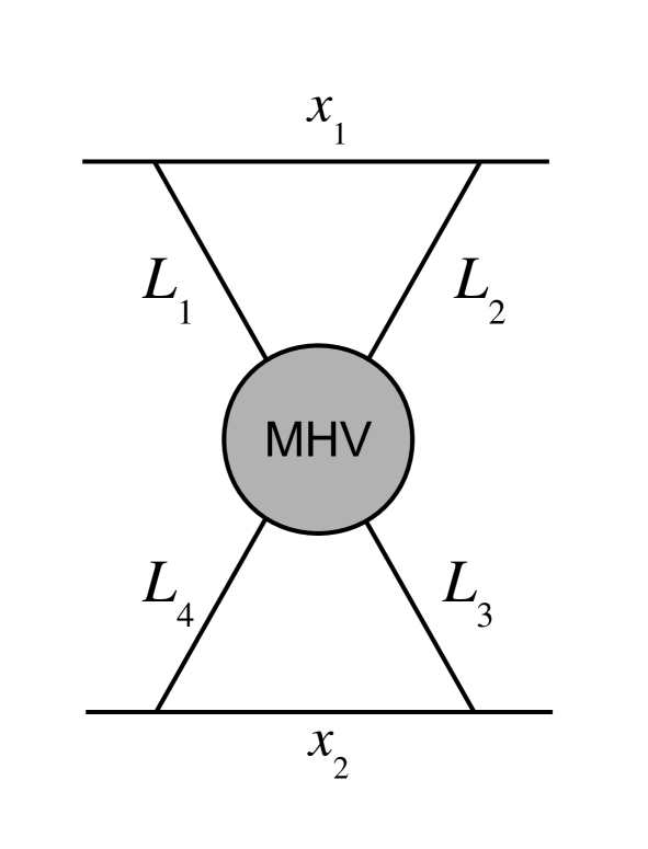
Figure 3: The single MHV diagram contributing to the dilatation operator at one loop.

It consists of one supersymmetric four-point MHV vertex,

$$V_{\rm MHV}(1,2,3,4)\ =\ {\delta^{(4)}(\sum_{i=1}^{4}L_{i})\delta^{(8)}(\sum_{i=1}^{4}\ell_{i}\eta_{i})\over\langle 12\rangle\langle 23\rangle\langle 34\rangle\langle 41\rangle}\,,$$ (3.6)

and four scalar propagators $1/(L_{1}^{2}\cdots L_{4}^{2})$ connecting it to the four scalars in the operators. Here $L_{i}$ are the (off-shell) momenta of the four particles in the vertex. The off-shell continuations of the spinors associated to the internal legs are defined using the prescription of [1], namely

$$\ell_{i\alpha}:=L_{i\alpha\dot{\alpha}}\xi^{\dot{\alpha}}\ .$$ (3.7)

Here $\xi^{\dot{\alpha}}$ is a constant reference spinor. Next we extract the relevant component vertices for the three flavour assignments in (3.5). These turn out to be:

$${\rm Tr}: \qquad\dfrac{\langle 13\rangle\langle 24\rangle}{\langle 12\rangle\langle 34\rangle}\,,$$

$$\mathbb{P}: \qquad-1\,,$$

$$\mbox{1 \kern-5.89996pt{\rm l}}: \qquad\dfrac{\langle 13\rangle\langle 24\rangle}{\langle 23\rangle\langle 14\rangle}\,.$$ (3.10)

Hence in the case of $\mathbb{P}$ the resulting loop integral is precisely the double-bubble integral $I(x_{12})$ of (2.7) (up to a sign), while in the other two cases the double-bubble integrand is dressed with the vertex factors in (3.10). In the following we discuss the additional contributions from the vertex for the three configurations ${\rm Tr}$, $\mathbb{P}$ and 1 l.

The Tr integrand

We begin our analysis with the vertex factor for the trace configuration, first line of (3.10). Using the off-shell prescription for MHV diagrams we can rewrite it as

$$T:={[\xi|L_{1}L_{3}|\xi]\,[\xi|L_{2}L_{4}|\xi]\over[\xi|L_{1}L_{2}|\xi]\,[\xi|L_{3}L_{4}|\xi]}\ .$$ (3.11)

Using momentum conservation to eliminate $L_{2}$ and $L_{4}$, this can be recast as a sum of three terms,

$$T\ =\ -{[\xi|L_{1}L_{3}|\xi]\over[\xi|L_{3}L|\xi]}-{[\xi|L_{1}L_{3}|\xi]\over[\xi|L_{1}L|\xi]}-{[\xi|L_{1}L_{3}|\xi]^{2}\over[\xi|L_{1}L|\xi]\,[\xi|L_{3}L|\xi]}\ ,$$ (3.12)

where $L:=L_{1}+L_{2}$. The first two terms correspond to linear bubble integrals in $L_{1}$ and $L_{3}$, respectively. We will study separately the contribution arising from the last term. The linear bubble integral is

$$\int\!{d^{D}K\over(2\pi)^{D}}{K^{\mu}\over K^{2}(K\pm L)^{2}}\ =\ \mp{L^{\mu}\over 2}{\rm Bub}(L^{2})\,,$$ (3.13)

where

$${\rm Bub}(L^{2}):=\int\!{d^{D}K\over(2\pi)^{D}}{1\over K^{2}(K+L)^{2}}\ .$$ (3.14)

This is one of the two scalar bubbles comprising the MZ integral of Figure 2. In the following we will then only quote the coefficient dressing the MZ integral. Doing so, the first term in (3.12) becomes, after the reduction,

$$-{[\xi|LL_{3}|\xi]\over[\xi|L_{3}L|\xi]}\cdot{1\over 2}\ =\ {1\over 2}\,.$$ (3.15)

Similarly, the second term in (3.12) gives a result of $+1/2$. Next we move to the third term. To simplify its expression, we first notice that the bubble integral in $L_{1}$ is symmetric under the transformation $L_{1}\to L-L_{1}$. The idea is then to simplify the integrand by using this symmetry. Thus, we rewrite the quantity $[\xi|L_{1}L_{3}|\xi]$ in the numerator as $[\xi|L_{1}L_{3}|\xi]\ =\ [\xi|(L_{1}-{1\over 2}L)L_{3}|\xi]+{1\over 2}[\xi|LL_{3}|\xi]$. Doing so, we get

$$-{[\xi|L_{1}L_{3}|\xi]^{2}\over[\xi|L_{1}L|\xi]\,[\xi|L_{3}L|\xi]}=-{[\xi|(L_{1}-{L\over 2})L_{3}|\xi]^{2}\over[\xi|L_{1}L|\xi]\,[\xi|L_{3}L|\xi]}+{1\over 4}{[\xi|LL_{3}|\xi]\over[\xi|L_{1}L|\xi]}+{[\xi|(L_{1}-{1\over 2}L)L_{3}|\xi]\over[\xi|L_{1}L|\xi]}\ .$$ (3.16)

We then notice that the first and the second term are antisymmetric under the transformation $L_{1}\to L-L_{1}$ and hence vanish upon integration. The third term is a sum of two linear bubbles in $L_{3}$, and the corresponding contributions are quickly seen to be equal to $-1/2$ and zero, respectively.

Summarising, the trace integral gives a contribution of $1/2$ times the dimensionally regularised MZ integral. Thus ${\cal A}_{\rm UV}={1/2}$.

The $\mathbb{P}$ integrand

In this case the vertex is simply $-1$ and the corresponding result is $-1$ times the MZ integral, or ${\cal B}_{\rm UV}=-1$.

The 1 l integrand

The relevant vertex factor is written in the third line of (3.10). In this case we observe that

$${\langle 13\rangle\langle 24\rangle\over\langle 23\rangle\langle 14\rangle}\ =\ 1+{\langle 12\rangle\langle 34\rangle\over\langle 23\rangle\langle 14\rangle}\ .$$ (3.17)

The first term gives a contribution equal to the MZ integral, and we will now argue that the second term is UV finite, and hence does not contribute to the dilatation operator. Indeed, we can write

$${\langle 12\rangle\langle 34\rangle\over\langle 23\rangle\langle 14\rangle}\ =\ {[\xi|L_{1}L|\xi][\xi|L_{3}L|\xi]\over[\xi|(L-L_{1})L_{3}|\xi][\xi|L_{1}(L+L_{3})|\xi]}\ .$$ (3.18)

The UV divergences we are after arise when $L_{1}$ and $L_{3}$ are large. The integrand (3.18) provides one extra power of momentum per integration, which makes each of the two bubbles in the MZ integral finite. Thus ${\cal C}_{\rm UV}=1$.

We end this section with a couple of comments.

1. Since MHV diagrams are obtained from a particular axial gauge choice, combined with a field redefinition [3, 4], it is guaranteed that $\xi$-dependence drops out at the end of the calculation. In the present case one can see this directly as follows. Lorentz invariance ensures that the result of the $L_{1}$- and $L_{3}$-integrations can only depend on $L^{2}$, as the other Lorentz-invariant quantity $[\xi|L^{2}|\xi]$ vanishes (note that $L\cdot\xi$ cannot appear as our integrands only depend on the anti-holomorphic spinor $\xi_{\dot{\alpha}}$).

2. We point out that in the MHV diagram formalism there are no self-energy corrections to the propagator, as already observed in Section 6 of [5]. Presumably this is also the case for the self-energy evaluated with the twistor action of [14] employed in [11] for the calculation of the one-loop dilatation operator. It is interesting to note that the superfield renormalisation in the lightcone gauge formalism of [16] is finite in the ${\cal N}=4$ theory.

4 Conclusions

We conclude with some suggestions for future investigations.

Firstly, it would be interesting to apply MHV diagrams to the calculation of the dilatation operator in other sectors of ${\cal N}=4$ SYM, also containing fermions and derivatives. Applications to different Yang-Mills theories with less supersymmetry can also be considered, given the validity of the MHV diagram method beyond ${\cal N}=4$ SYM.

An obvious goal is the extension of our calculation to higher loops. This has proved difficult for amplitudes, but addressing the calculation of just the UV-divergent part of the two-point correlation function may simplify this task enormously. At one loop the complete dilatation operator is known [17], while direct perturbative calculations at higher loops – without the assumption of integrability – have been performed only up to two [18, 19, 20], three [21, 22, 23] and four loops [24] in particular sectors. A simplified route to such a calculation would be greatly desirable, and would provide further verification of this crucial assumption. The expected structure remains that of (2.7), with the double-bubble integral replaced by more complicated (but still single-scale) loop integrals.

It would also be very interesting if one could apply other on-shell methods such as generalised unitarity [25, 26] to the direct calculation of two-point functions, and hence to the dilatation operator of ${\cal N}=4$ SYM.

Finally, our result hints at a link between the Yangian symmetry of amplitudes in ${\cal N}=4$ SYM [27] and integrability of the dilatation operator of the theory [2, 17, 28, 29, 30, 31]. It would be interesting to explore this point further.

We hope to be able to report on some of these ideas in the very near future.

References

- [1] F. Cachazo, P. Svrcek, and E. Witten, “MHV vertices and tree amplitudes in gauge theory,” JHEP 0409 (2004) 006, arXiv:hep-th/0403047 [hep-th].
- [2] J. Minahan and K. Zarembo, “The Bethe ansatz for N=4 super Yang-Mills,” JHEP 0303 (2003) 013, arXiv:hep-th/0212208 [hep-th].
- [3] P. Mansfield, “The Lagrangian origin of MHV rules,” JHEP 0603 (2006) 037, arXiv:hep-th/0511264 [hep-th].
- [4] A. Gorsky and A. Rosly, “From Yang-Mills Lagrangian to MHV diagrams,” JHEP 0601 (2006) 101, arXiv:hep-th/0510111 [hep-th].
- [5] A. Brandhuber, B. Spence, and G. Travaglini, “One-loop gauge theory amplitudes in N=4 super Yang-Mills from MHV vertices,” Nucl.Phys. B706 (2005) 150–180, arXiv:hep-th/0407214 [hep-th].
- [6] J. Bedford, A. Brandhuber, B. Spence, and G. Travaglini, “A Twistor approach to one-loop amplitudes in N=1 supersymmetric Yang-Mills theory,” Nucl.Phys. B706 (2005) 100–126, arXiv:hep-th/0410280 [hep-th].
- [7] C. Quigley and M. Rozali, “One-loop MHV amplitudes in supersymmetric gauge theories,” JHEP 0501 (2005) 053, arXiv:hep-th/0410278 [hep-th].
- [8] J. Bedford, A. Brandhuber, B. Spence, and G. Travaglini, “Non-supersymmetric loop amplitudes and MHV vertices,” Nucl.Phys. B712 (2005) 59–85, arXiv:hep-th/0412108 [hep-th].
- [9] A. Brandhuber, B. Spence, and G. Travaglini, “From trees to loops and back,” JHEP 0601 (2006) 142, arXiv:hep-th/0510253 [hep-th].
- [10] A. Brandhuber, B. Spence, and G. Travaglini, “Tree-Level Formalism,” J.Phys. A44 (2011) 454002, arXiv:1103.3477 [hep-th].
- [11] L. Koster, V. Mitev, and M. Staudacher, “A Twistorial Approach to Integrability in N=4 SYM,” arXiv:1410.6310 [hep-th].
- [12] M. Wilhelm, “Amplitudes, Form Factors and the Dilatation Operator in SYM Theory,” arXiv:1410.6309 [hep-th].
- [13] R. Boels, L. Mason, and D. Skinner, “Supersymmetric Gauge Theories in Twistor Space,” JHEP 0702 (2007) 014, arXiv:hep-th/0604040 [hep-th].
- [14] R. Boels, L. Mason, and D. Skinner, “From twistor actions to MHV diagrams,” Phys.Lett. B648 (2007) 90–96, arXiv:hep-th/0702035 [hep-th].
- [15] T. Adamo and L. Mason, “MHV diagrams in twistor space and the twistor action,” Phys.Rev. D86 (2012) 065019, arXiv:1103.1352 [hep-th].
- [16] A. Belitsky, S. E. Derkachov, G. Korchemsky, and A. Manashov, “Dilatation operator in (super-)Yang-Mills theories on the light-cone,” Nucl.Phys. B708 (2005) 115–193, arXiv:hep-th/0409120 [hep-th].
- [17] N. Beisert, “The complete one loop dilatation operator of N=4 super Yang-Mills theory,” Nucl.Phys. B676 (2004) 3–42, arXiv:hep-th/0307015 [hep-th].
- [18] B. Eden, “A Two-loop test for the factorised S-matrix of planar N = 4,” Nucl.Phys. B738 (2006) 409–424, arXiv:hep-th/0501234 [hep-th].
- [19] A. Belitsky, G. Korchemsky, and D. Mueller, “Integrability of two-loop dilatation operator in gauge theories,” Nucl.Phys. B735 (2006) 17–83, arXiv:hep-th/0509121 [hep-th].
- [20] G. Georgiou, V. Gili, and J. Plefka, “The two-loop dilatation operator of N=4 super Yang-Mills theory in the SO(6) sector,” JHEP 1112 (2011) 075, arXiv:1106.0724 [hep-th].
- [21] N. Beisert, “The dynamic spin chain,” Nucl.Phys. B682 (2004) 487–520, arXiv:hep-th/0310252 [hep-th].
- [22] B. Eden, C. Jarczak, and E. Sokatchev, “Three-loop test of the dilatation operator and integrability in N = 4 SYM,” Fortsch.Phys. 53 (2005) 610–614.
- [23] C. Sieg, “Superspace computation of the three-loop dilatation operator of N=4 SYM theory,” Phys.Rev. D84 (2011) 045014, arXiv:1008.3351 [hep-th].
- [24] N. Beisert, T. McLoughlin, and R. Roiban, “The Four-loop dressing phase of N=4 SYM,” Phys.Rev. D76 (2007) 046002, arXiv:0705.0321 [hep-th].
- [25] Z. Bern, L. J. Dixon, and D. A. Kosower, “One loop amplitudes for e+ e- to four partons,” Nucl.Phys. B513 (1998) 3–86, arXiv:hep-ph/9708239 [hep-ph].
- [26] R. Britto, F. Cachazo, and B. Feng, “Generalized unitarity and one-loop amplitudes in N=4 super-Yang-Mills,” Nucl.Phys. B725 (2005) 275–305, arXiv:hep-th/0412103 [hep-th].
- [27] J. M. Drummond, J. M. Henn, and J. Plefka, “Yangian symmetry of scattering amplitudes in N=4 super Yang-Mills theory,” JHEP 0905 (2009) 046, arXiv:0902.2987 [hep-th].
- [28] N. Beisert, C. Kristjansen, and M. Staudacher, “The Dilatation operator of conformal N=4 super Yang-Mills theory,” Nucl.Phys. B664 (2003) 131–184, arXiv:hep-th/0303060 [hep-th].
- [29] I. Bena, J. Polchinski, and R. Roiban, “Hidden symmetries of the AdS(5) x S**5 superstring,” Phys.Rev. D69 (2004) 046002, arXiv:hep-th/0305116 [hep-th].
- [30] N. Beisert and M. Staudacher, “The N=4 SYM integrable super spin chain,” Nucl.Phys. B670 (2003) 439–463, arXiv:hep-th/0307042 [hep-th].
- [31] N. Beisert, “The Dilatation operator of N=4 super Yang-Mills theory and integrability,” Phys.Rept. 405 (2004) 1–202, arXiv:hep-th/0407277 [hep-th].