Dynamical quenching with non-local $\alpha$ and downward pumping

Abstract

In light of new results, the one-dimensional mean-field dynamo model of Brandenburg & Käpylä (2007) with dynamical quenching and a nonlocal Babcock–Leighton $\alpha$ effect is re-examined for the solar dynamo. We extend the one-dimensional model to include the effects of turbulent downward pumping (Kitchatinov & Olemskoy 2011), and to combine dynamical quenching with shear. We use both the conventional dynamical quenching model of Kleeorin & Ruzmaikin (1982) and the alternate one of Hubbard & Brandenburg (2011), and confirm that with varying levels of non-locality in the $\alpha$ effect, and possibly shear as well, the saturation field strength can be independent of the magnetic Reynolds number.

1 Introduction

The generation of large-scale magnetic fields is usually explained in terms of mean-field theory, in which one considers solutions of the averaged induction equation (Parker 1979; Krause & Rädler 1980). In this theory, the evolution of the mean magnetic field is governed by turbulent transport coefficients such as the $\alpha$ effect and the turbulent magnetic diffusivity $\eta_{\rm t}$. As long as the magnetic field is small compared with the equipartition field strength $B_{\rm eq}$, and if there is also helicity in the system, one expects the parameter $\alpha$, which drives dynamo action, to be of the order of the rms velocity of the turbulence, and $\eta_{\rm t}$ to be of the order of the rms velocity times the mixing or correlation length of the turbulence (Moffatt 1978). If this is indeed true, the relevant time scale of the problem should be the dynamical time scale, rather than the microscopic diffusion time which would be longer than the dynamical one by a factor that is equal to the magnetic Reynolds number $R_{\rm m}$, which in turn is very large in many systems of astrophysical relevance; $10^{6}$ to $10^{9}$ in the Solar convection zones.

Early attempts to determine $\alpha$ and $\eta_{\rm t}$ from simulations have suggested that this may not be so simple, and that the saturated field strength might decrease rapidly with increasing $R_{\rm m}$ in a phenomenon called “catastrophic quenching” (Cattaneo & Vainshtein 1991; Cattaneo & Hughes 1996). The reason for this is that magnetic helicity, which measures the twist of magnetic flux bundles, obeys a conservation equation (Gruzinov & Diamond 1994). So, as the physics of the $\alpha$ effect describes the twisting of the large-scale magnetic field by helical fluid motions, it is constrained by the magnetic helicity equation in a fashion which resists further twisting of the field. This is possible because magnetic helicity is signed: by producing magnetic helicity at small scale of opposite sign, magnetic helicity can remain constant even while dynamo action creates helical large scale fields.

In the mean-field formalism, this can be described by an $\alpha$ effect that depends not only on background fluid motions, but also on the helicity of the small-scale magnetic field. This provides an extra evolution equation for the magnetic $\alpha$ effect which describes the production of magnetic helicity locally where strong mean field twisting occurs. This approach goes back to the early work of Kleeorin & Ruzmaikin (1982), and is now usually referred to as the dynamical quenching formalism. This formalism has been found to describe many properties of direct numerical simulations of turbulent dynamos (Field & Blackman 2002; Blackman & Brandenburg 2002; Subramanian 2002).

This formalism is quite different from “algebraic” $\alpha$ quenching that is often invoked to describe saturation of the magnetic field by reducing $\alpha$ locally, depending on the amplitude of the mean field at that position. The dynamical quenching formalism can even produce an $\alpha$ effect where there was none to begin with, for example in the turbulent decay of a helical large-scale magnetic field (Yousef et al. 2003; Kemel et al. 2011; Blackman & Subramanian 2013). This can also occur when a mean magnetic field is produced by the shear–current effect (Rogachevskii & Kleeorin 2003, 2004). While the shear–current effect is quite different from the $\alpha$ effect of dynamo theory, it produces a helical mean field, and therefore must be accompanied by the generation of small-scale magnetic helicity so that no net magnetic helicity is produced. This has been demonstrated within the dynamical quenching formalism (Brandenburg & Subramanian 2005), where a magnetic $\alpha$ effect was produced, even though there is no kinetic $\alpha$ effect. Further examples are the so-called interface dynamos (Parker 1993), where shear operates at the bottom of the solar convection zone, and the kinetic $\alpha$ effect operates at its top. Again, a magnetic $\alpha$ is produced at locations where strong twisting of the mean field occurs, regardless of the location of the kinetic $\alpha$ effect, as was demonstrated by simulations in spherical geometry (Chatterjee et al. 2010).

This situation is similar to models with a Babcock–Leighton $\alpha$ effect which acts at the surface based on magnetic fields at the bottom of the convection zone (e.g. Charbonneau 2010). This effect is therefore highly non-local. Dynamical quenching in such a model was considered by Brandenburg & Käpylä (2007; hereafter BK07). There, dynamical quenching was found to lead to catastrophic quenching, i.e., the saturation field strength was found to decrease like $R_{\rm m}^{-1}$. Subsequent work of Kitchatinov & Olemskoy (2011, 2012) has now shown that, using a more realistic model of the solar dynamo, catastrophic quenching may be alleviated in the presence of strong downward pumping. An alternate new line of research has shown that the “standard” set of dynamical quenching equations can fail in the presence of shear (Hubbard & Brandenburg 2011). The purpose of the present paper is to examine both recent results in the context of the idealized model of BK07, determining both whether the results of KO11 depend on a more complicated geometry and how more recent formulations of dynamical alpha quenching behave in the presence of non-local phenomena.

2 Dynamical $\alpha$ quenching and non-locality

In mean field theory we decompose the fields into mean (overbar) and fluctuating (lower case) quantities, so for example the magnetic field can be written as

$${\vec{B}}=\overline{\vec{B}}+{\vec{b}},$$ (1)

where $\overline{{\vec{b}}}=0$. Defining the mean turbulent electromotive force

$$\overline{\vec{\cal E}}\equiv\overline{{\vec{u}}\times{\vec{b}}},$$ (2)

we can write the mean field induction equation (Parker 1979; Krause & Rädler 1980)

$${\partial\overline{\vec{B}}\over\partial t}=\mbox{\boldmath$\nabla$}{}\times\left(\overline{\vec{U}}\times\overline{\vec{B}}+\overline{\vec{\cal E}}-\eta\mu_{0}\overline{\vec{J}}\right).$$ (3)

However, if there is helicity in the system, there is also the occurrence of a magnetic $\alpha$ effect, $\alpha_{\rm M}$, which characterizes the production of internal twist in the system and is governed by

$${\partial\alpha_{\rm M}\over\partial t}+\mbox{\boldmath$\nabla$}{}\cdot\overline{\mbox{\boldmath${\cal F}$}}{}=-2\eta_{\rm t}k_{\rm f}^{2}\left({\overline{\vec{\cal E}}\cdot\overline{\vec{B}}\over B_{\rm eq}^{2}}+{\alpha_{\rm M}\over R_{\rm m}}\right),$$ (4)

as described in (Brandenburg & Subramanian 2005). $\overline{\mbox{\boldmath${\cal F}$}}{}$ is the mean flux of small scale magnetic helicity.

In this paper, $\overline{\vec{\cal E}}$ is assumed to have contributions from the kinetic and magnetic $\alpha$ effects, $\alpha_{\rm K}$ and $\alpha_{\rm M}$, respectively, the turbulent magnetic diffusivity $\eta_{\rm t}$, and the turbulent pumping or $\gamma$ effect, i.e., we write

$$\overline{\vec{\cal E}}=\hat{\alpha}_{\rm K}\circ\overline{\vec{B}}+\alpha_{\rm M}\overline{\vec{B}}+{\vec{\gamma}}\times\overline{\vec{B}}-\eta_{\rm t}\overline{\vec{J}}.$$ (5)

We are studying the effect of a non-local Babcock Leighton type $\alpha$, which generates an $\overline{\vec{\cal E}}$ that is restricted to the surface layers of the Sun, but depends only on the mean magnetic field deep within the convective zone. Therefore, we treat the kinetic $\alpha$ effect as nonlocal integral kernel, $\hat{\alpha}_{\rm K}$, and

$$\hat{\alpha}_{\rm K}\circ\overline{\vec{B}}=\int_{z_{1}}^{z_{2}}\hat{\alpha}_{\rm K}(z,z^{\prime})\overline{\vec{B}}(z^{\prime},t)\,{\rm d}{}z^{\prime}$$ (6)

denotes a convolution, which is here restricted to be only in $z$.

For simplicity, we use a Cartesian domain, with the $xy$ plane corresponding to surfaces of constant radius in the Sun, and $z$ corresponding to the radial direction. We have restricted ourselves to $xy$ averages in the Cartesian domain, so $\overline{\vec{B}}=\overline{\vec{B}}(z,t)$ depends only on $z$ and $t$, and we assume that the turbulent pumping parameter ${\vec{\gamma}}=\gamma\mbox{\boldmath$z$}{}$ only acts in the vertical direction. Note that the magnetic helicity equation is unaffected by the $\gamma$ effect – just like the large-scale velocity term, $\overline{\vec{U}}\times\overline{\vec{B}}$, it does not directly affect the evolution of $\alpha_{\rm M}$.

The possibility of nonlocal $\alpha$ and $\eta_{\rm t}$ effects has been inferred also from simulations of magneto-rotational turbulence in accretion discs (Brandenburg & Sokoloff 2002) and for turbulence (Brandenburg et al. 2008). In principle, $\eta_{\rm t}$ and $\gamma$ should of course also be nonlocal, but this will here be neglected. Following BK07, we restrict ourselves to a simple expression of the form

$$\hat{\alpha}_{\rm K}(z,z^{\prime})=\alpha_{0}\,g_{\rm out}(z)\,g_{\rm in}(z^{\prime}),$$ (7)

where $\alpha_{0}$ is a coefficient, to be specified below, and

$$g_{\rm out}(z)={\textstyle{1\over 2}}\left[1+\mbox{\rm erf}\left({z-z_{2}\over d}\right)\right],$$ (8)

$$g_{\rm in}(z^{\prime})={\textstyle{1\over 2}}\left[1-\mbox{\rm erf}\left({z^{\prime}-z_{1}\over d}\right)\right]$$ (9)

are simple profile functions representing the peak of the source function near $z=z_{2}$ with a sensitivity for fields located near $z=z_{1}$. For the following we choose $-z_{1}=z_{2}=2.5/k_{1}$ and $d=0.05/k_{1}$ in the domain $-\pi<k_{1}z<\pi$; see Fig. 1. Here, $k_{1}$ is the smallest wavenumber in the computational domain and is used as our inverse unit length.

Figure 1: Contributions $g_{\rm in}(z)$ and $g_{\rm out}(z)$ entering the nonlocal $\alpha$ effect defined in Eq. (7). The dotted lines indicate the positions of $z_{1}$ and $z_{2}$.

In most of the published literature on dynamical quenching, the magnetic helicity flux has no contribution from a term $\overline{\vec{\cal E}}\times\overline{\vec{A}}$, which enters with opposite signs in the evolution equations for the magnetic helicity flux from small-scale and large-scale fields. However, recent work (Hubbard & Brandenburg 2011,2012) now reveals that this is not permissible, and including it tends to alleviate catastrophic quenching. Nonetheless, for comparison with the published literature, we solve Eqs. (3) and (4) first for the case $\overline{\mbox{\boldmath${\cal F}$}}{}=0$. We use an implicit scheme for $\alpha_{\rm M}$, as described in BK07. We have considered a model using linear shear of the form $\overline{\vec{U}}(z)=(0,S(z)x,0)$. In this paper, $\gamma$ and $\eta_{\rm t}$ are assumed constant. The strength of shear, $\alpha$, and $\gamma$ effects is quantified by the non-dimensional numbers

$$C_{S}={S\over\eta_{\rm t}k_{1}^{2}},\quad C_{\alpha}={\alpha_{0}\over\eta_{\rm t}k_{1}},\quad C_{\gamma}={\gamma\over\eta_{\rm t}k_{1}}.$$ (10)

In the following we use $C_{S}=100$, $C_{\alpha}=0.1$, and $k_{\rm f}/k_{1}=5$, while $C_{\gamma}$ will be varied. In many cases an explicit treatment of the $\alpha_{\rm M}$ equation suffices (e.g. Blackman & Brandenburg 2002), but in the present case an explicit solution algorithm was found to be unstable; see BK07 for details.

Figure 2: Dependence of the saturation field strength on $C_{\gamma}$ for $R_{\rm m}=10^{4}$.

2.1 Homogeneous shear

While the Sun has a strong shear layer at the base of the convective zone, we first consider the case of homogeneous shear ($C_{S}$ not depending on $z$). In this case, it turns out that the inclusion of downward pumping in the model of BK07 makes the dynamo stronger, as can be seen in Fig. 2, where we show that $\overline{\vec{B}}^{2}\propto\gamma^{2}$. The reason for this is that most of the field is generated in the middle of the domain, while most of the quenching via $\alpha_{\rm M}$ occurs near the top of the layer around $z=z_{2}$; see Fig. 3. Nevertheless, this model still experiences catastrophic quenching; see Fig. 4. These results are quite similar to those obtained for local $\alpha$ profiles (Brandenburg & Subramanian 2005). We note that for $R_{\rm m}>10^{4}$ it is important to perform the calculations using double precision arithmetics.

Figure 3: Vertical dependence of $\overline{\vec{B}}^{2}$, $\overline{\vec{J}}\cdot\overline{\vec{B}}$, and $\alpha_{\rm M}$ for a model with homogeneous shear, all normalized by their local extrema, for different values of $C_{\gamma}$.

Figure 4: Dependence of the saturation field strength on $R_{\rm m}$ for models with homogeneous shear, with and without downward pumping or $\gamma$ effect.

A somewhat surprising property of the present solutions is the fact that $\overline{\vec{J}}\cdot\overline{\vec{B}}$ is still negative everywhere; see the middle panel of Fig. 3. This is mainly a consequence of the nonlocal $\alpha$ effect; for a local $\alpha$ effect, and certainly in the absence of shear, $\overline{\vec{J}}\cdot\overline{\vec{B}}$ would always be positive for positive $\alpha$. Nevertheless, $\alpha_{\rm M}$ is negative everywhere, the opposite sign as the kinetic $\alpha$ effect, so there is no possibility of having anti-quenching anywhere in the domain.

Figure 5: Saturation behavior of a dynamo with a shear profile that is identical to that of $g_{\rm in}$, which is localized only to the lower layer.

2.2 Shear layer

Next, inspired by the solar tachocline, we consider a model where shear is confined to a narrow layer at the bottom of the domain. In that case we replace $S$ by $S(z)=S_{0}g_{\rm in}$, i.e., the shear layer coincides with the profile with which the $\alpha$ kernel operates on the magnetic field. It turns out that in that case the magnetic field becomes oscillatory. This means that $\alpha_{\rm M}$ can now change sign and thereby offset the quenching such that the saturation level becomes independent of the magnetic field strength. This is shown in Fig. 5, where we plot $\langle\overline{\vec{B}}^{2}\rangle$ versus time for two values of $R_{\rm m}$. Both the linear growth rate and the initial saturation field strength are now found to be independent of $R_{\rm m}$. (For smaller values of $R_{\rm m}$ the linear growth rate would become progressively smaller, because the effective dynamo number would decrease.) For $R_{\rm m}=10^{3}$ the model saturates at a fixed level for all times, but in models with larger values of $R_{\rm m}$ ($10^{4}$ or $10^{5}$) the field achieves only temporary saturation before it grows beyond any limit. This is in agreement with earlier models of Kitchatinov & Olemskoy (2011) and other dynamical quenching models, for example in models of Brandenburg & Subramanian (2005), in which an $\alpha_{\rm M}$ is driven by a magnetic helicity flux of Vishniac–Cho type (Vishniac & Cho 2001).

3 Alternate quenching

Figure 6: Dynamo behavior at early times with homogeneous shear using the alternate quenching formulation. $C_{S}=-100$, $C_{\alpha}=-0.1$, $C_{\gamma}=-1$, $R_{\rm m}=10^{5}$. Note the difference in the scale of the $x$-axes, the dynamo waves are too numerous to plot fully. Further, the energy in the top left panel is a running mean.

Quite different results are obtained when a different formulation of dynamical $\alpha$ quenching is used. Using the results in Hubbard & Brandenburg (2011,2012), we can replace Eq. (4) with

$$\partial\overline{h}/\partial t=-2\eta\left(\overline{\vec{J}}\cdot\overline{\vec{B}}+\alpha_{M}B_{\rm eq}^{2}/\eta_{\rm t}\right)$$ (11)

$$\alpha_{M}=\eta_{\rm t}k_{\rm f}^{2}\left(\overline{h}-\overline{\vec{A}}\cdot\overline{\vec{B}}\right)/B_{\rm eq}^{2}.$$ (12)

This formulation gives better results in the geometries studied in Hubbard & Brandenburg (2012), namely shearing-periodic with a homogeneous $\alpha$ effect. This approach has now also been applied to solar-like models in spherical geometry (Pipin et al. 2013).

In this case, it is important to consider how an oscillatory dynamo functions. First the $x$-component of the field at the bottom, $B_{x}^{\rm bot}$, is sheared into a $y$-directed field $B_{y}^{\rm bot}$ with ${\rm sgn}\,{}B_{y}^{\rm bot}={\rm sgn}\,{}SB_{x}^{\rm bot}$. In the assumed high-shear regime ($|C_{S}|\gg C_{\alpha},C_{\gamma}$), this $y$ directed toroidal field dominates the energetics. From this toroidal field the non-local $\alpha$-effect generates an $x$-directed poloidal field $B_{x}^{\rm top}$ at the top, with ${\rm sgn}\,{}B_{x}^{\rm top}={\rm sgn}\,{}(-\alpha^{\prime}SB_{x}^{\rm bot})$, where the prime denotes a $z$ derivative due to taking the curl in Eq. (3). If ${\rm sgn}\,{}B_{x}^{\rm top}\neq{\rm sgn}\,{}B_{x}^{\rm bot}$, then when the field is transported downwards (via pumping through the gamma effect, or diffusion), it will counter the original field, resulting in dynamo waves, as seen in Fig. 6. If the signs are the same, there is only amplification, with no back-reaction mechanism available in the formalism we consider, although algebraic quenching or similar must eventually play a significant role. In this section we therefore only present results for the oscillatory case.

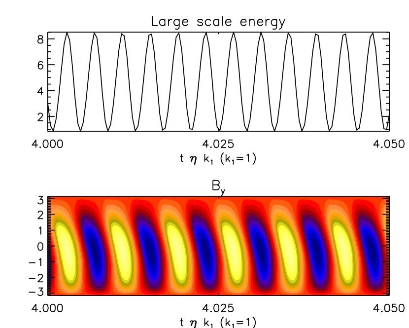
Figure 7: Dynamo behavior at intermediate times with homogeneous shear for a dynamo with $C_{S}=-100$, $C_{\alpha}=-0.1$, $C_{\gamma}=-1$, $R_{\rm m}=500$. The alternate quenching formulation was used. Here the energy is not a running mean.

This nonlocal $\alpha\Omega$ dynamo does not have the same behavior as a uniform one. Perhaps most significantly, the energy in the magnetic fields shows strong fluctuations as the magnetic field oscillates. Accordingly, for most figures in this section, our energies are running means. The exception is Fig. 7, where we show a time-magnification of the dynamo, and strong time variation is visible.

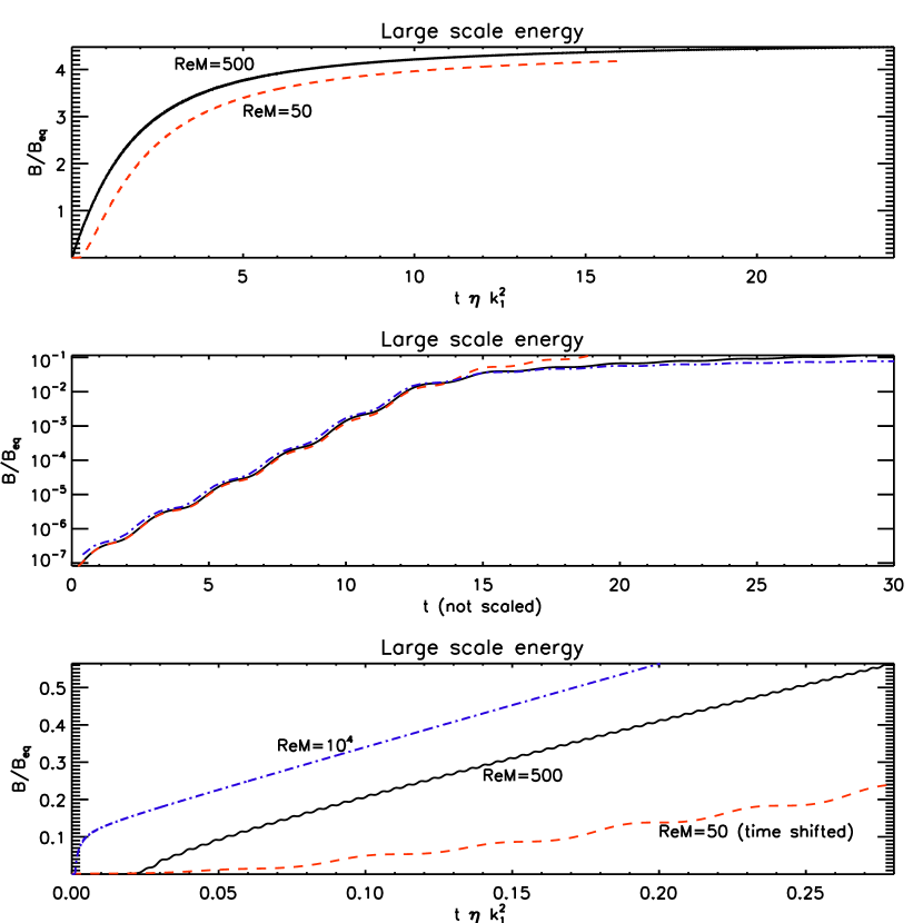
Figure 8: Alternate quenching dynamo behaviors for three values of $R_{\rm m}$, other parameters $S=-100$, $\alpha=-0.1$, $\gamma=-1$. Black/solid: $R_{\rm m}=500$; red/dashed: $R_{\rm m}=50$; blue/dash-dotted: $R_{\rm m}=10^{4}$ (not included in top panel).

In Fig. 8 we examine the dependency of the system on $R_{\rm m}$. In the top panel, we see that the time dependence is similar for $R_{\rm m}=50,\ 500$, although it appears that $R_{\rm m}=50$ is not yet in the asymptotically high $R_{\rm m}$ regime. Note that the time axis is scaled to the resistive time. In the middle panel, we show the early (kinematic) behavior, which is identical for all three values of $R_{\rm m}=50,\ 500,\ 10^{4}$, with a non-scaled time axis. In the bottom panel, we see the early non-linear evolution, where the results for $R_{\rm m}=500,\ 10^{4}$ are identical, but again it appears that $R_{\rm m}=50$ is too low for fully asymptotic behavior. Note that the time of entrance into the linear growth regime is different for the three cases because of the scaling of $t$. Intriguingly, the slow-saturation phase shown is similar to that predicted for closed helical systems. We see no evidence for a declining final field strength with $R_{\rm m}$.

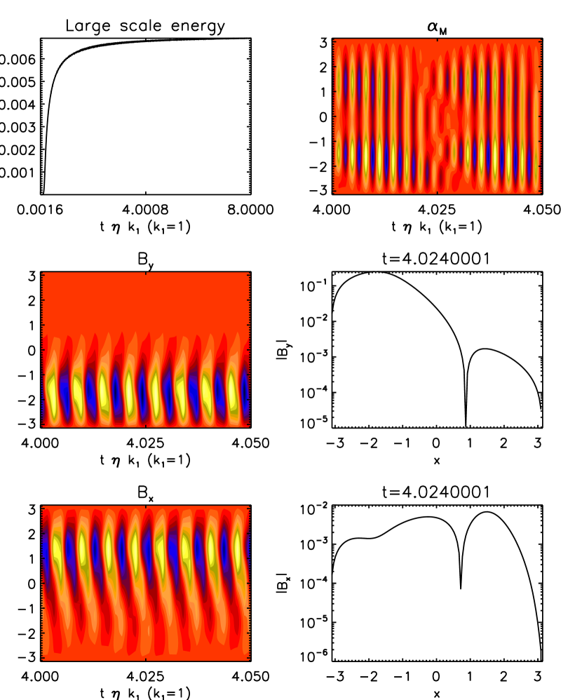
Figure 9: Alternate quenching dynamo behavior at intermediate times with inhomogeneous shear. $C_{S}=-100$, $C_{\alpha}=-0.2$, $C_{\gamma}=-1$, $R_{\rm m}=500$. Notably, here the shear is not homogeneous, instead it has the same spatial variation as $g_{\rm in}$. The dynamo control parameters had to be changed ($C_{\alpha}$ from $-0.1$ to $-0.2$) to allow dynamo growth. The dips in the temporal log-linear cuts are sign-changes.

As a final comment in this section, in Fig. 9 we include a run with not merely a non-local $\alpha$ effect, but also non-local shear, to model a Babcock-Leighton $\alpha$ effect at the surface, and the strong shear localized in the solar tachocline. The dynamo is overall similar to the case with homogeneous shear but, predictably, far less strongly excited, necessitating an increased magnitude of $C_{\alpha}=-0.2$

4 Conclusions

The present work has demonstrated that, within the framework of the dynamical quenching model, a nonlocal $\alpha$ effect of Babcock-Leighton type combined with downward pumping can alleviate catastrophic quenching only when the shear layer is separated from the layer where the Babcock-Leighton $\alpha$ acts. Downward pumping can lead to a strong enhancement of the dynamo even in models where shear is uniform. While this can compensate for some of the field reduction suffered from large values of $R_{\rm m}$, it nevertheless does not change the $R_{\rm m}^{-1}$ scaling.

The model of Kitchatinov & Olemskoy (2011) contains an important feature that is found here only in time-dependent cases, namely the sign reversal of $\alpha_{\rm M}$ in some places, which leads to catastrophic anti-quenching (or amplification). Similar sign reversals of the local value of $\alpha_{\rm M}$ have been seen in some earlier models with a local $\alpha$ effect (Guerrero et al. 2010; Chatterjee et al. 2011), but it needs to be seen whether this behavior is physically realistic and still compatible with the original equations.

Further, it is clearly only a simplification to neglect the flux term in Eq. (4). Even though the domain may be closed, we must always expect there to be internal magnetic helicity fluxes resulting from the inhomogeneity of the model. Magnetic helicity fluxes between local extrema in the small-scale magnetic helicity density and across the equator have been detected in direct numerical simulations (Mitra et al. 2010; Hubbard & Brandenburg 2010; Del Sordo et al. 2013). Such fluxes might well be sufficient for alleviating catastrophic quenching without the need for invoking the non-locality of $\alpha$.

On the other hand, an improved integration of shear with dynamical quenching can avoid catastrophic $\alpha$-quenching, but only functions and generates an oscillatory dynamo when the signs of the $\alpha$ effect and the shear are the same. When the signs are different, dynamical quenching predicts no feedback, so the field grows without bound (although some form of geometric $\alpha$ quenching must eventually control the system).

- [1] Blackman, E. G., Brandenburg, A.: 2002, ApJ 579, 359
- [2] Blackman, E. G., & Subramanian, K.: 2013, MNRAS 429, 1398
- [3] Brandenburg, A., & Käpylä, P. J.: 2007, New J. Phys. 9, 305 (BK07)
- [4] Brandenburg, A., Rädler, & K.-H., Schrinner, M.: 2008, A&A 482, 739
- [5] Brandenburg, A., & Sokoloff, D.: 2002, GApFD 96, 319
- [6] Brandenburg, A., & Subramanian, K.: 2005, AN 326, 400
- [7] Cattaneo, F., & Hughes, D. W.: 1996, Phys Rev E 54, R4532
- [8] Cattaneo, F., & Vainshtein, S. I.: 1991, ApJ 376, L21
- [9] Charbonneau, P.: 2010, Living Rev. Solar Phys. 7, 3
- [10] Chatterjee, P., Brandenburg, A., & Guerrero, G.: 2010, GApFD 104, 591
- [11] Chatterjee, P., Guerrero, G., & Brandenburg, A.: 2011, A&A 525, A5
- [12] Del Sordo, F., Guerrero, G., & Brandenburg, A.: 2013, MNRAS 429, 1686
- [13] Field, G. B., & Blackman, E. G.: 2002, ApJ 572, 685
- [14] Gruzinov, A. V., & Diamond, P. H.: 1994, Phys Rev Lett 72, 1651
- [15] Guerrero, G., Chatterjee, P., & Brandenburg, A.,: 2010, MNRAS 409, 1619
- [16] Hubbard, A., & Brandenburg, A.: 2010, GApFD 104, 577
- [17] Hubbard, A., & Brandenburg, A.: 2011, ApJ 727, 11
- [18] Hubbard, A., & Brandenburg, A.: 2012, ApJ 748, 51
- [19] Kemel, K., Brandenburg, A., & Ji, H.: 2011, Phys Rev E 84, 056407
- [20] Kleeorin, N. I., & Ruzmaikin, A. A.: 1982, Magnetohydrodynamics 18, 116
- [21] Kitchatinov, L. L., & Olemskoy, S. V.: 2011, AN 332, 496
- [22] Kitchatinov, L. L., & Olemskoy, S. V.: 2012, Solar Phys. 276, 3
- [23] Krause, F., & Rädler, K.-H.: 1980, Mean-field magnetohydrodynamics and dynamo theory (Pergamon Press, Oxford)
- [24] Mitra, D., Candelaresi, S., Chatterjee, P., Tavakol, R., & Brandenburg, A.: 2010, AN 331, 130
- [25] Moffatt, H. K.: 1978, Magnetic field generation in electrically conducting fluids (Cambridge University Press, Cambridge)
- [26] Parker, E. N.: 1979, Cosmical magnetic fields (Clarendon Press, Oxford)
- [27] Parker, E. N.: 1993, ApJ 408, 707
- [28] Pipin, V. V., Sokoloff, D. D., Zhang, H., & Kuzanyan, K. M.: 2013, ApJ 768, 46
- [29] Rogachevskii, I., & Kleeorin, N.: 2003, Phys Rev E 68, 036301
- [30] Rogachevskii, I., & Kleeorin, N.: 2004, Phys Rev E 70, 046310
- [31] Subramanian, K.: 2002, Bull. Astr. Soc. India 30, 715
- [32] Vishniac, E. T., & Cho, J.: 2001, ApJ 550, 752
- [33] Yousef, T. A., Brandenburg, A., & Rüdiger, G.: 2003, A&A 411, 321