1 Introduction

1.1 Multiple Andreev reflections

During last decade considerable progress has been made in the investigation and understanding the mechanisms of current transport in mesoscopic superconducting junctions. The term mesoscopic here refers to the junctions where bulk superconducting electrodes in equilibrium (reservoirs) are connected by small non-superconducting region with the size smaller than any inelastic mean free path. Such junctions include metallic atomic-size contacts, tunnel junctions, diffusive (metallic) and ballistic (2D electron gas) SNS junctions. A common feature of all these structures concerns the fact that the quasiparticles injected in the junction at zero temperature cannot escape into the reservoir unless the applied voltage is larger than the superconducting energy gap in the reservoir, $eV>2\Delta$. In 1963, Schrieffer and Wilkins suggested that the necessary energy for the quasiparticle transmission at subgap voltage, $eV<2\Delta$ can be provided by transferring Cooper pairs between the reservoirs [1].

The microscopic mechanism for such multiparticle transport, multiple Andreev reflections (MAR), was suggested in 1982 by Klapwijk, Blonder, and Tinkham [2, 3]. According to the MAR scenario formulated in terms of the scattering theory, injected quasiparticles repeatedly undergo Andreev reflections from the superconducting reservoirs, gaining energy $eV$ during each traversal of the junction, which allows them to eventually escape from the junction, see Fig. 1. As the result, a spectral flow across the energy gap is generated, which creates strongly non-equilibrium quasiparticle distribution within the contact area. This mechanism explains the nature of the dissipative current in voltage biased junctions. Also it allows one to anticipate considerable enhancement of the current shot noise. Indeed, transmission of one quasiparticle across the energy gap at applied voltage $V$ requires $N=\mathop{\mbox{Int}}(2\Delta/eV)$ Andreev reflections [Int($x$) denoting the integer part of $x$], which transfer the total charge, $q^{\it{eff}}=(N+1)e$, between the electrodes. This enhancement of the transmitted charge gives rise to the enhancement of the current shot noise compared to the case of normal junction, according to the Schottky formula, $S=2q^{\it{eff}}I$, where $S$ is the spectral density of the noise at zero frequency.

                       

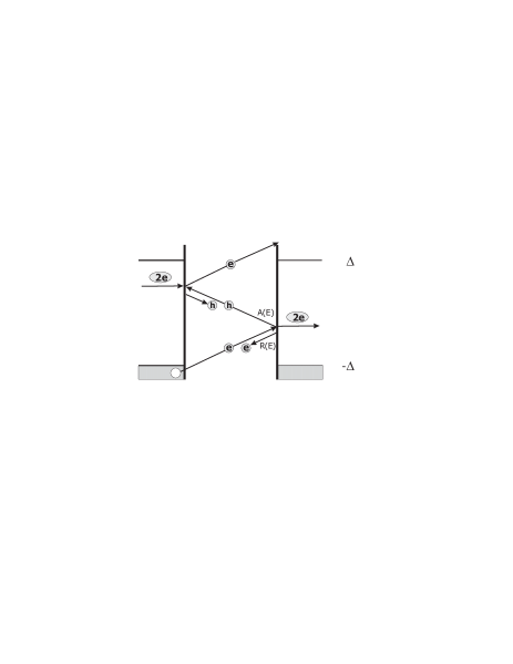
Figure 1.  : Multiple Andreev reflections in superconducting junction. Quasiparticle energy increases by $eV$ after every traversal of the junction, generating spectral flow across the energy gap, $(-\Delta,\Delta)$. At the interface, quasiparticle undergoes Andreev reflection with probability $A(E)$, and normal reflection with probability $R(E)$.

The mechanism of MAR is general for all kinds of superconducting junctions. However, the MAR transport regime appears differently in junctions having small and large lengths. In short junctions where the distance between the superconducting electrodes is small compared to the superconducting coherence length, $\xi_{0}=\hbar v_{F}/\Delta$, such as point contacts and tunnel junctions, consequent Andreev reflections are fully coherent. Essential feature of this coherent MAR regime is the ac Josephson effect, and also highly non-linear $I$-$V$ characteristics with the subharmonic gap structure (SGS) – sequence of current structures at voltages $eV=2\Delta/n$ ($n$ is an integer) [4].

The same features, the ac Josephson effect and SGS, appear also in ballistic SNS junctions and short diffusive SNS junctions [5, 6]. In diffusive SNS junctions, the electron-hole coherence in the normal metal persists over a distance of the coherence length $\xi_{E}=\sqrt{\hbar{\cal D}/2E}$ from the superconductor (${\cal D}$ is the diffusion constant). The overlap of coherent proximity regions induced by both SN interfaces creates an energy gap in the electron spectrum of the normal metal. In short junctions with a small length $d$ compared to the coherence length, $d\ll\xi_{\Delta}$, and with a large proximity gap of the order of the energy gap $\Delta$ in the superconducting electrodes, the phase coherence covers the entire normal region.

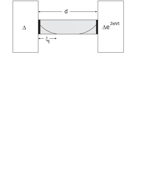
Figure 2.  : Proximity effect in long diffusive SNS junctions. Shaded region indicates diffusive metal connecting superconducting reservoirs marked with $\Delta$; bold lines indicate interface resistances. Superconducting correlations exponentially decay over length $\xi_{E}$, which is small compared to the junction length $d$

Rather different, incoherent MAR regime occurs in long diffusive SNS junctions with a small proximity gap of the order of Thouless energy $E_{{\it Th}}={\hbar\cal D}/d^{2}\ll\Delta$ [7]. If $E_{{\it Th}}$ is also small on a scale of applied voltage, $E_{{\it Th}}\ll eV$, then the coherence length $\xi_{E}$ is much smaller than the junction length at all relevant energies $E\sim\mathop{\mathrm{m}in}(eV,\Delta)$. In this case, the proximity regions near the SN interfaces become virtually decoupled, as shown in Fig. 2, and the Josephson current oscillations are strongly suppressed. At the same time, the quasiparticle distribution inside the energy gap is strongly non-equilibrium as soon as an inelastic mean free path exceeds the junction length, $l_{\varepsilon}\gg d$, because the subgap electrons must undergo many (incoherent) Andreev reflections before they enter the reservoir.

It is interesting that in the junctions with transparent interfaces, the complex transport mechanism of incoherent MAR is not clearly revealed by $I$-$V$ characteristics of the junction, which are close to the Ohm’s law. Thus the excess shot noise becomes the central characteristic of interest in this regime. Quasi-linear behavior of $I$-$V$ characteristics in the incoherent MAR regime can be understood from the following argument. The MAR transport in real space through the junction with normal resistance $R_{N}$ is associated with a spectral current flow along the energy axis through a series of $N+1$ resistors with the total effective resistance $R=(N+1)R_{N}$. Since only electrons incoming within the energy layer $eV$ below the gap edge, $-\Delta$, participate in the MAR transport, the spectral current $I_{p}$ is given by the equation $I_{p}=V/R$. However, each pair of consecutive Andreev reflections transfers the charge $2e$ through the junction, and the real current $I$ is therefore $N+1$ times larger than the spectral current: $I=(N+1)I_{p}=V/R_{N}$. It is clear from this argument, that particular nature of the normal resistance (e.g. tunnel resistance instead of diffusive metallic resistance) plays no essential role in the behavior of the current.

1.2 Current shot noise

Shot noise in mesoscopic conductors has been extensively studied during recent years (for a review see [8]). In ballistic normal electron systems with tunnel barriers, the shot noise is produced by electron tunnelling through the barriers, and it is described by the Schottky formula $S=2eI$ [9]. In diffusive metallic wires the shot noise is due to elastic electron scattering by the impurities, and in this case, an additional factor $1/3$ appears in the Schottky formula, $S=(2/3)eI$ [10, 11, 12]. This Fano factor is modified in long wires whose length exceeds the inelastic scattering length due to the effect of electron-electron and electron-phonon relaxation [10, 13, 14].

In normal-superconducting (NS) systems, the current shot noise produced by the impurity scattering is enhanced at subgap voltages, $eV<\Delta$, by the factor of two compared to the normal conductors [15, 16]. This is because the subgap current transport involves one Andreev reflection, which results in the transfer through the junction of an elementary charge $2e$, instead of $e$. More elaborated analysis shows further enhancement of the shot noise at small voltage due to the contribution of the proximity region near the NS interface [17].

In superconducting junctions, the shot noise power is tremendously enhanced at small voltage by the factor $q^{\it{eff}}/e\sim 2\Delta/eV\gg 1$, because of the MAR. For the coherent MAR regime this effect has been well theoretically established [18, 19, 20] and experimentally investigated [21, 22, 23]. For the incoherent MAR regime, similar effect of the shot noise enhancement has been theoretically predicted in Refs. [25, 26, 27]. The experimental observation of multiply enhanced shot noise in long SNS junctions was reported in Refs. [23, 24, 28]. Although there is the same mechanism of the noise enhancement in both cases, there is remarkable difference between the behavior of the noise power at small voltage in the ballistic and diffusive junctions. In the ballistic junctions, the current exponentially decreases with voltage [4] while the effective charge grows inversely proportionally to the voltage, hence the shot noise power also exponentially decreases. On the other hand, in the diffusive junctions, the current decay follows a power law. In particular, in the incoherent MAR regime, the current approximately follows the Ohm’s law, and therefore the noise power approaches a constant value at zero voltage, $S\sim\Delta/R_{N}$. This effect, which results from the enhanced effective charge, can be also explained as the result of strong electron non-equilibrium distribution developed by the MAR process with an effective noise temperature $T_{0}\sim\Delta$.

The finite noise level at zero voltage is a very interesting property of the incoherent MAR regime, which can be employed for the investigation of the effect of inelastic relaxation on MAR. The MAR transport regime assumes the time spent by a quasiparticle within the junction area, $\tau_{{\it dwell}}$, to be small compared to the inelastic relaxation time $\tau_{\varepsilon}$. However, at $eV\rightarrow 0$, the dwelling time infinitely increases because of MAR, and inelastic relaxation unavoidably starts to play a role. The inelastic scattering suppresses the spectral flow upwards in energy generated by MAR, and thus the MAR regime is destroyed. As the result, the normal region of the junction becomes an equilibrium reservoir, and the SNS junction turns into two NS junctions connected in series. This is manifested by the decrease of the noise level at small voltage, the cross over being controlled by the ratio $\tau_{\varepsilon}/\tau_{{\it dwell}}$. Precisely this behavior of the shot noise has been observed in the experiment [24, 28]. It is important that because of the absence of the Josephson effect in the incoherent MAR regime, a small-voltage region of the dissipative current branch, $E_{Th}\ll eV\ll\Delta$, can be experimentally accessed without switching to the Josephson branch.

In this paper, we outline a theory of the current shot noise in the incoherent MAR regime. We will discuss the “collisionless” limit of perfect MAR as well as the effect of inelastic relaxation. While theoretical analysis of the current shot noise in the coherent MAR regime can be done on the basis of the scattering theory [18, 19, 29], the present case requires different approach, which operates with electron and hole diffusion flows rather than with ballistic quasiparticle trajectories, and considers the Andreev reflections as the relationships between these diffusive flows rather than the scattering events. Such formalism has been developed in Ref. [7], and it is outlined in the next section.

2 Circuit theory of incoherent MAR

2.1 Microscopic background

The system under consideration consists of a normal channel ($0\!<\!x\!<\!d$) confined between two voltage biased superconducting electrodes, with the elastic mean free path $\ell$ much shorter than any characteristic size of the problem. In this limit, the microscopic analysis of current transport can be performed in the framework of the diffusive equations of nonequilibrium superconductivity [30] for the $4\!\times\!4$ matrix Keldysh-Green function ${\check{G}}(t_{1}t_{2},x)$,

$$\displaystyle[\check{H},\check{G}]=i\hbar{\cal D}\partial_{x}\check{J},\quad\check{J}=\check{G}\partial_{x}\check{G},\quad{\check{G}}^{2}=\check{1},$$ (1)

$$\displaystyle\check{H}=\check{1}[i\hbar\sigma_{z}\partial_{t}-e\phi(t)+\hat{\Delta}(t)],\quad\hat{\Delta}=\Delta e^{i\sigma_{z}\chi}i\sigma_{y},$$ (2)

where $\Delta,\chi$ are the modulus and the phase of the order parameter, and $\phi$ is the electric potential. The Pauli matrices $\sigma_{i}$ operate in the Nambu space of $2\!\times\!2$ matrices denoted by “hats”, the products of two-time functions are interpreted as their time convolutions. The electric current $I$ per unit area is expressed through the Keldysh component $\hat{J}^{K}$ of the matrix current $\check{J}$,

$$I(t)=(\pi\hbar\sigma_{N}/4e)\mathop{\mathrm{Tr}}\sigma_{z}\hat{J}^{K}(tt,x),$$ (3)

where $\sigma_{N}$ is the conductivity of the normal metal.

At the SN interface, the matrix ${\check{G}}$ satisfies the boundary condition [31]

$$\left(\sigma_{N}\check{J}\right)_{\pm 0}=\left(2R_{SN}\right)^{-1}\left[{\check{G}}_{-0},{\check{G}}_{+0}\right],$$ (4)

where the indices $\pm 0$ denote the right and left sides of the interface and $R_{SN}$ is the interface resistance per unit area in the normal state. Within the model of infinitely narrow potential of the interface barrier, $U(x)=H\delta(x)$, the interface resistance is related to the barrier strength $Z=H(\hbar v_{F})^{-1}$ as $R_{SN}=2\ell Z^{2}/3\sigma_{N}$ [32]. It has been shown in Ref. [33] that Eq. (4) is valid either for a completely transparent interface ($R_{SN}\rightarrow 0$, ${\check{G}}_{+0}={\check{G}}_{-0}$) or for an opaque barrier whose resistance is much larger than the resistance $R(\ell)=\ell/\sigma_{N}$ of a metal layer with the thickness formally equal to $\ell$.

According to the definition of the matrix ${\check{G}}$,

$${\check{G}}=\left(\begin{array}[]{ccc}\hat{g}^{R}&\hat{G}^{K}\\ 0&\hat{g}^{A}\end{array}\right),\;\hat{G}^{K}=\hat{g}^{R}\hat{f}-\hat{f}\hat{g}^{A},$$ (5)

Eqs. (1) and (4) represent a compact form of separate equations for the retarded and advanced Green’s functions $\hat{g}^{R,A}$ and the distribution function $\hat{f}=f_{+}+\sigma_{z}f_{-}$. Their time evolution is imposed by the Josephson relation $\chi(t)=2eVt$ for the phase of the order parameter in the right electrode (we assume $\chi=0$ in the left terminal). This implies that the function $\check{G}(t_{1}t_{2},x)$ consists of a set of harmonics $\check{G}(E_{n},E_{m},x)$, $E_{n}=E+neV$, which interfere in time and produce the ac Josephson current. However, when the junction length $d$ is much larger than the coherence length $\xi_{E}$ at all relevant energies, we may consider coherent quasiparticle states separately at both sides of the junction, neglecting their mutual interference and the ac Josephson effect. Thus, the Green’s function in the vicinity of left SN interface can be approximated by the solution $\hat{g}=\sigma_{z}\cosh\theta+i\sigma_{y}\sinh\theta$ of the static Usadel equations for a semi-infinite SN structure [34], with the spectral angle $\theta(E,x)$ satisfying the equation

$$\tanh[\theta(E,x)/4]=\tanh[\theta_{N}(E)/4]\exp(-x/\xi_{E}\sqrt{i}),$$ (6)

with the boundary condition

$$W\sqrt{i\Delta/E}\sinh(\theta_{N}-\theta_{S})+2\sinh(\theta_{N}/2)=0.$$ (7)

The indices $S$, $N$ in these equations refer to the superconducting and the normal side of the interface, respectively.

The dimensionless parameter $W$ in Eq. (7),

$$W={R(\xi_{\Delta})\over R_{SN}}={\xi_{\Delta}\over dr},\quad r={R_{SN}\over R_{N}},$$ (8)

where $R_{N}=R(d)=d/\sigma_{N}$ is the resistance of the normal channel per unit area, has the meaning of an effective barrier transmissivity for the spectral functions [35]. Note that even at large barrier strength $Z\gg 1$ ensuring the validity of the boundary conditions Eq. (4) [33], the effective transmissivity $W\sim(\xi_{\Delta}/\ell)Z^{-2}$ of the barrier in a “dirty” system, $\ell\ll\xi_{\Delta}$, could be large. In this case, the spectral functions are virtually insensitive to the presence of a barrier and, therefore, the boundary conditions Eqs. (4) can be applied to an arbitrary interface if we approximately consider highly transmissive interfaces with $W>\xi_{\Delta}/\ell\gg 1$ as completely transparent, $W=\infty$.

The distribution functions $f_{\pm}(E,x)$ are to be considered as global quantities within the whole normal channel determined by the kinetic equations

$$\partial_{x}[D_{\pm}(E,x)\partial_{x}f_{\pm}(E,x)]=0,$$ (9)

with dimensionless diffusion coefficients

$$\displaystyle D_{+}=(1/4)\mathop{\mathrm{Tr}}\left(1-\hat{g}^{R}\hat{g}^{A}\right)=\cos^{2}\mathop{\mathrm{Im}}\theta,$$ (10)

$$\displaystyle D_{-}=(1/4)\mathop{\mathrm{Tr}}\left(1-\sigma_{z}\hat{g}^{R}\sigma_{z}\hat{g}^{A}\right)=\cosh^{2}\mathop{\mathrm{Re}}\theta.$$

Assuming the normal conductance of electrodes to be much larger than the junction conductance, we consider them as equilibrium reservoirs with unperturbed spectrum, $\theta_{S}=\mathop{\mathrm{Arctanh}}(\Delta/E)$, and equilibrium quasiparticle distribution, $\hat{f}_{S}(E)=f_{0}(E)\equiv\tanh(E/2T)$. Within this approximation, the boundary conditions for the distribution functions at $x=0$ read

$$\sigma_{N}D_{+}\partial_{x}f_{+}(E,0)=G_{+}(E)[f_{+}(E,0)-f_{0}(E)],$$ (11)

$$\sigma_{N}D_{-}\partial_{x}f_{-}(E,0)=G_{-}(E)f_{-}(E,0),$$ (12)

where

$$G_{\pm}(E)=R_{SN}^{-1}\left(N_{S}N_{N}\mp M_{S}^{\pm}M_{N}^{\pm}\right),$$ (13)

$$N(E)=\mathop{\mathrm{Re}}(\cosh\theta),\;M^{+}(E)+iM^{-}(E)=\sinh\theta.$$ (14)

At large energies, $|E|\gg\Delta$, when the normalized density of states $N(E)$ approaches unity and the condensate spectral functions $M^{\pm}(E)$ turn to zero at both sides of the interface, the conductances $G_{\pm}(E)$ coincide with the normal barrier conductance; within the subgap region $|E|<\Delta$, $G_{+}(E)=0$.

Similar considerations are valid for the right NS interface, if we eliminate the time dependence of the order parameter in Eq. (1), along with the potential of right electrode, by means of a gauge transformation [36]

$${\check{G}}(t_{1}t_{2},x)=\exp(i\sigma_{z}eVt_{1})\widetilde{{\check{G}}}(t_{1}t_{2},x)\exp(-i\sigma_{z}eVt_{2}).$$ (15)

As a result, we arrive at the same static equations and boundary conditions, Eqs. (6)-(14), with $x\rightarrow d-x$, for the gauge-transformed functions $\widetilde{\hat{g}}(E,x)$ and $\widetilde{\hat{f}}(E,x)$. Thus, to obtain a complete solution, e.g. for the distribution function $f_{-}$, which determines the dissipative current,

$$I={\sigma_{N}\over 2e}\int_{-\infty}^{\infty}dE\,D_{-}\partial_{x}f_{-},$$ (16)

one must solve the boundary problem for ${\hat{f}}(E,x)$ at the left SN interface, and a similar boundary problem for $\widetilde{\hat{f}}(E,x)$ at the right interface, and then match the distribution function asymptotics deep inside the normal region by making use of the relationship following from Eqs. (5), (15),

$${\hat{f}}(E,x)=\widetilde{\hat{f}}(E+\sigma_{z}eV,x).$$ (17)

2.2 Circuit representation of boundary conditions

In order for this kinetic scheme to conform to the conventional physical interpretation of Andreev reflection in terms of electrons and holes, we introduce the following parametrization of the matrix distribution function,

$$\hat{f}(E,x)=1-2\left(\begin{array}[]{ccc}n^{e}(E,x)&0\\ 0&n^{h}(E,x)\end{array}\right),$$ (18)

where $n^{e}$ and $n^{h}$ will be considered as the electron and hole population numbers. Deep inside the normal metal region, they acquire rigorous meaning of distribution functions of electrons and holes, and approach the Fermi distribution in equilibrium. In this representation, Eqs. (9) take the form

$$D_{\pm}(E,x)\partial_{x}n_{\pm}(E,x)=\mbox{const}\equiv-I_{\pm}(E)/\sigma_{N},$$ (19)

where $n_{\pm}=n^{e}\pm n^{h}$, and they may be interpreted as conservation equations for the (specifically normalized) net probability current $I_{+}$ of electrons and holes, and for the electron-hole imbalance current $I_{-}$. Furthermore, the probability currents of electrons and holes, defined as $I^{e,h}=(1/2)(I_{+}\pm I_{-})$, separately obey the conservation equations. The probability currents $I^{e,h}$ are naturally related to the electron and hole diffusion flows, $I^{e,h}=-\sigma_{N}\partial_{x}n^{e,h}$, at large distances $x\gg\xi_{E}$ from the SN boundary. Within the proximity region, $x<\xi_{E}$, each current $I^{e,h}$ generally consists of a combination of both the electron and hole diffusion flows, which reflects coherent mixing of normal electron and hole states in this region,

$$I^{e,h}=-(\sigma_{N}/2)\left[(D_{+}\pm D_{-})\partial_{x}n^{e}+(D_{+}\mp D_{-})\partial_{x}n^{h}\right].$$ (20)

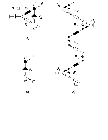
Figure 3.  : Elementary equivalent circuits representing boundary conditions in Eq. (21) for the electron and hole population numbers $n^{e,h}(E,0)$ and probability currents $I^{e,h}(E)$, at energies outside the gap, $|E|>\Delta$ (a), and within the subgap region, $|E|<\Delta$ (b); equivalent network in ($x,E$)-space for incoherent MAR in SNS junction (c). Filled and empty symbols stand for electron- and hole- related elements, respectively; half-filled squares denote Andreev resistors; $U_{n}=n_{F}(E_{n})$.

In terms of electrons and holes, the boundary conditions in Eqs. (11), (12) read

$$I^{e,h}=G_{T}\left(n_{F}-n^{e,h}\right)\mp G_{A}\left(n^{e}-n^{h}\right),$$ (21)

where

$$G_{T}=G_{+},\;G_{A}=(G_{-}-G_{+})/2.$$ (22)

Each of the equations (21) may be clearly interpreted as a Kirchhoff rule for the electron or hole probability current flowing through the effective circuit (tripole) shown in Fig. 3(a). Within such interpretation, the nonequilibrium populations of electrons and holes $n^{e,h}$ at the interface correspond to “potentials” of nodes attached to the “voltage source” – the Fermi distribution $n_{F}(E)$ in the superconducting reservoir – by “tunnel resistors” $R_{T}(E)=G_{T}^{-1}(E)$. The “Andreev resistor” $R_{A}(E)=G_{A}^{-1}(E)$ between the nodes provides electron-hole conversion (Andreev reflection) at the SN interface.

The circuit representation of the diffusive SN interface is analogous to the scattering description of ballistic SN interfaces: the tunnel and Andreev resistances play the same role as the normal and Andreev reflection coefficients in the ballistic case [32]. For instance, at $|E|>\Delta$ [Fig. 3(a)], the probability current $I^{e}$ is contributed by equilibrium electrons incoming from the superconductor through the tunnel resistor $R_{T}$, and also by the current flowing through the Andreev resistor $R_{A}$ as the result of hole-electron conversion. Within the subgap region, $|E|<\Delta$ [Fig. 3(b)], the quasiparticles cannot penetrate into the superconductor, $R_{T}=\infty$, and the voltage source is disconnected, which results in detailed balance between the electron and hole probability currents, $I^{e}=-I^{h}$ (complete reflection). For the perfect interface, $R_{A}$ turns to zero, and the electron and hole population numbers become equal, $n^{e}=n^{h}$ (complete Andreev reflection). The nonzero value of the Andreev resistance for $R_{SN}\neq 0$ accounts for suppression of Andreev reflection due to the normal reflection by the interface.

Detailed information about the boundary resistances can be obtained from their asymptotic expressions in Ref. [7]. In particular, $R_{\pm}(E)$ turns to zero at the gap edges due to the singularity in the density of states which enhances the tunnelling probability. The resistance $R_{-}(E)$ approaches the normal value $R_{SN}$ at $E\rightarrow 0$ due to the enhancement of the Andreev reflection at small energies, which results from multiple coherent backscattering of quasiparticles by the impurities within the proximity region.

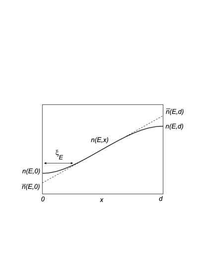
Figure 4.  : Qualitative behavior of population numbers within the normal channel (solid curve). The edge distortions of the linear $x$-dependence of population numbers, Eq. (23), occur within the proximity regions. The difference between the boundary population numbers $n(E,0)$, $n(E,d)$ and their effective values $\overline{n}(E,0)$, $\overline{n}(E,d)$ for true normal electrons and holes is included in the renormalization of the boundary resistances, Eq. (26).

The proximity effect can be incorporated into the circuit scheme by the following way. We note that the diffusion coefficients $D_{\pm}$ in Eq. (10) turn to unity far from the SN boundary, and therefore the population numbers $n^{e,h}$ become linear functions of $x$,

$$n^{e,h}(E,x)\approx{\overline{n}}^{e,h}(E,0)-R_{N}I^{e,h}(E)x/d.$$ (23)

This equation defines the renormalized population numbers ${\overline{n}}^{e,h}(E,0)$ at the NS interface, which differ from $n^{e,h}(E,0)$ due to the proximity effect, as shown in Fig. 4. These quantities have the meaning of the true electron/hole populations which would appear at the NS interface if the proximity effect had been switched off. It is possible to formulate the boundary conditions in Eq. (21) in terms of these population numbers by including the proximity effect into renormalization of the tunnel and Andreev resistances. To this end, we will associate the node potentials with renormalized boundary values $\overline{n}^{e,h}(E,0)=(1/2)[\overline{n}_{+}(E,0)\pm\overline{n}_{-}(E,0)]$ of the population numbers, where ${\overline{n}}_{\pm}(E,0)$ are found from the exact solutions of Eqs. (19),

$${\overline{n}}_{\pm}(E,0)=n_{\pm}(E,0)-m_{\pm}(E)I_{\pm}(E).$$ (24)

Here $m_{\pm}(E)$ are the proximity corrections to the normal metal resistance at given energy for the probability and imbalance currents, respectively,

$$m_{\pm}(E)=\pm R_{N}\int_{0}^{\infty}{dx\over d}\left|D_{\pm}^{-1}(E,x)-1\right|.$$ (25)

It follows from Eq. (24) that the same Kirchhoff rules as in Eqs. (21), (22) hold for ${\overline{n}}^{e,h}(E,0)$ and $I^{e,h}(E)$, if the bare resistances $R_{\pm}$ are substituted by the renormalized ones,

$$R_{\pm}(E)\rightarrow\overline{R}_{\pm}(E)=R_{\pm}(E)+m_{\pm}(E).$$ (26)

In certain cases, there is an essential difference between the bare and renormalized resistances, which leads to qualitatively different properties of the SN interface for normal electrons and holes compared to the properties of the bare boundary. Let us first discuss a perfect SN interface with $R_{SN}\rightarrow 0$. Within the subgap region $|E|<\Delta$, the bare tunnel resistance $R_{T}$ is infinite whereas the bare Andreev resistance $R_{A}$ turns to zero; this corresponds to complete Andreev reflection, as already explained. However, the Andreev resistance for normal electrons and holes, $\overline{R}_{A}(E)=2m_{-}(E)$, is finite and negative, which leads to enhancement of the normal metal conductivity within the proximity region [38, 39]. At $|E|>\Delta$, the bare tunnel resistance $R_{T}$ is zero, while the renormalized tunnel resistance $\overline{R}_{T}(E)=m_{+}(E)$ is finite (though rapidly decreasing at large energies). This leads to suppression of the probability currents of normal electrons and holes within the proximity region, which is to be attributed to the appearance of Andreev reflection. Such a suppression is a global property of the proximity region in the presence of sharp spatial variation of the order parameter, and it is similar to the over-the-barrier Andreev reflection in the ballistic systems. In the presence of normal scattering at the SN interface, the overall picture depends on the interplay between the bare interface resistances $R_{\pm}$ and the proximity corrections $m_{\pm}$; for example, the renormalized tunnel resistance $\overline{R}_{T}(E)$ diverges at $|E|\rightarrow\Delta$, along with the proximity correction $m_{+}(E)$, in contrast to the bare tunnel resistance $R_{T}(E)$. This indicates complete Andreev reflection at the gap edge independently of the transparency of the barrier, which is similar to the situation in the ballistic systems where the probability of Andreev reflection at $|E|=\Delta$ is always equal to unity.

2.3 MAR networks

To complete the definition of an equivalent MAR network, we have to construct a similar tripole for the right NS interface and to connect boundary values of population numbers (node potentials) using the matching condition in Eq. (17) expressed in terms of electrons and holes,

$$n^{e,h}(E,x)=\widetilde{n}^{e,h}(E\pm eV,x).$$ (27)

Since the gauge-transformed distribution functions $\widetilde{f}_{\pm}$ obey the same equations Eq. (9)-(14), the results of the previous Section can be applied to the functions $\widetilde{n}^{e,h}(E)$ and $-\widetilde{I}^{e,h}(E)$ (the minus sign implies that $\widetilde{I}$ is associated with the current incoming to the right-boundary tripole). In particular, the asymptotics of the gauge-transformed population numbers far from the right interface are given by the equation

$$\widetilde{n}^{e,h}(E,x)\approx\widetilde{\overline{n}}^{e,h}(E,d)+R_{N}\widetilde{I}^{e,h}(E)\left(1-x/d\right).$$ (28)

After matching the asymptotics in Eqs. (23) and (28) by means of Eq. (27), we find the following relations,

$$I^{e,h}(E)=\widetilde{I}^{e,h}(E\pm eV),$$ (29)

$$\overline{n}^{e,h}(E,0)-\widetilde{\overline{n}}^{e,h}(E\pm eV,d)=R_{N}I^{e,h}(E).$$ (30)

From the viewpoint of the circuit theory, Eq. (30) may be interpreted as Ohm’s law for the resistors $R_{N}$ which connect energy-shifted boundary tripoles, separately for the electrons and holes, as shown in Fig. 3(c).

The final step which essentially simplifies the analysis of the MAR network, is based on the following observation. The spectral probability currents $I^{e,h}$ yield opposite contributions to the electric current in Eq. (16),

$$I={1\over 2e}\int_{-\infty}^{\infty}dE\left[I^{e}(E)-I^{h}(E)\right],$$ (31)

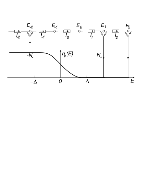
Figure 5.  : MAR network of Fig. 3(c) in energy space. The nodes outside the gap are connected with the distributed voltage source $n_{F}(E)$ (bold curve); the subgap nodes are disconnected from the voltage source.

due to the opposite charge of electrons and holes. At the same time, these currents, referred to the energy axis, transfer the charge in the same direction, viz., from bottom to top of Fig. 3(c), according to our choice of positive $eV$. Thus, by introducing the notation $I_{n}(E)$ for an electric current entering the node $n$, as shown by arrows in Fig. 3(c),

$$I_{n}(E)=\left\{\begin{array}[]{ccc}I^{e}(E_{n-1}),&n=2k+1,\\ -I^{h}(E_{n}),&n=2k,\end{array}\right.,\quad E_{n}=E+neV,$$ (32)

we arrive at an “electrical engineering” problem of current distribution in an equivalent network in energy space plotted in Fig. 5, where the difference between electrons and holes becomes unessential. The bold curve in Fig. 5 represents a distributed voltage source – the Fermi distribution $n_{F}(E)$ connected periodically with the network nodes. Within the gap, $|E_{n}|<\Delta$, the nodes are disconnected from the Fermi reservoir and therefore all partial currents associated with the subgap nodes are equal.

Since all resistances and potentials of this network depend on $E_{n}=E+neV$, the partial currents obey the relationship $I_{n}(E)=I_{k}[E+(n-k)eV]$ which allows us to express the physical electric current, Eq. (31), through the sum of all partial currents $I_{n}$ flowing through the normal resistors $R_{N}$, integrated over an elementary energy interval $0<E<eV$,

$$I={1\over 2e}\int_{-\infty}^{\infty}\!\!\!dE\,[I_{1}(E)+I_{0}(E)]={1\over e}\int_{0}^{eV}\!\!\!dE\,J(E),\quad J(E)=\!\!\!\sum_{n=-\infty}^{+\infty}\!\!\!I_{n}(E).$$ (33)

The spectral density $J(E)$ is periodic in $E$ with the period $eV$ and symmetric in $E$, $J(-E)=J(E)$, which follows from the symmetry of all resistances with respect to $E$.

As soon as the partial currents are found, the population numbers can be recovered by virtue of Eqs. (19), (21), (23), and (32),

$$n^{e,h}(E,x)=\overline{n}^{e,h}(E,0)\mp R_{N}I_{1,0}(E)x/d,$$ (34)

$$\overline{n}^{e,h}(E,0)=n_{F}-(1/2)\left[\overline{R}_{+}(I_{1}-I_{0})\pm\overline{R}_{-}(I_{1}+I_{0})\right]$$ (35)

at $|E|>\Delta$. Within the subgap region, Eq. (35) is inapplicable due to the indeterminacy of product $\overline{R}_{+}(I_{1}-I_{0})$. In this case, one may consider the subgap part of the network as a voltage divider between the nodes nearest to the gap edges, having the numbers $-N_{-}$, $N_{+}$, respectively, where

$$N_{\pm}=\mbox{Int}[(\Delta\mp E)/eV]+1.$$ (36)

Then the boundary populations at $|E|<\Delta$ become

$$\overline{n}^{e,h}(E,0)=n^{L,R}(E_{\pm N_{\pm}})\pm I_{0}\left[N_{\pm}R_{N}+\sum_{k=1}^{N_{\pm}-1}R_{A}(E_{\pm k})\right],$$ (37)

where $R,L$ indicate the right (left) node of the tripole, irrespectively of whether it relates to the left (even $n$) or right (odd $n$) interface. The physical meaning of $n^{R,L}(E_{n})$, however, depends on the parity of $n$,

$$n^{R,L}(E_{n})=\left\{\begin{array}[]{ccc}\overline{n}^{e,h}(E_{n},0),&n=2k,\\ \widetilde{\overline{n}}^{h,e}(E_{n},d),&n=2k+1.\end{array}\right.$$ (38)

The values $n^{R,L}$ in Eq. (37) can be found from Eq. (35) which is generalized for any tripole of the network in Fig. 5 outside the gap as

$$n^{R,L}(E_{n})=n_{F}(E_{n})-{1\over 2}\left[\overline{R}_{+}(E_{n})(I_{n+1}-I_{n})\pm\overline{R}_{-}(E_{n})(I_{n+1}+I_{n})\right].$$ (39)

As follows from Eqs. (35), (37), the energy distribution of quasiparticles has a step-like form (Fig. 6), which is qualitatively similar to, but quantitatively different from that found in OTBK theory [3]. The number of steps increases at low voltage, and the shape of the distribution function becomes resemblant to a “hot electron” distribution with the effective temperature of the order of $\Delta$. This distribution is modulated due to the discrete nature of the heating mechanism of MAR, which transfers the energy from an external voltage source to the quasiparticles by energy quanta $eV$.

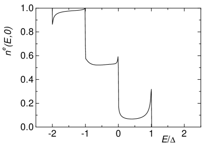
Figure 6.  : Energy dependence of the electron population number $n^{e}(E,0)$ at the left interface of the SNS junction with $R_{SN}=R_{N}$ and $d=5\xi_{\Delta}$, at $V=\Delta/e$ and $T=0$.

The circuit formalism can be simply generalized to the case of different transparencies of NS interfaces, as well as to different values of $\Delta$ in the electrodes. In this case, the network resistances become dependent not only on $E_{n}$ but also on the parity of $n$. As a result, the periodicity of the current spectral density doubles: $J(E)=J(E+2eV)$, and, therefore, $J(E)$ is to be integrated in Eq. (33) over the period $2eV$, with an additional factor $1/2$.

3 Current shot noise in the MAR regime

3.1 Noise of normal conductor

The main source of the shot noise in long diffusive SNS junctions with transparent interfaces ($R_{NS}\ll R_{N}$) is the impurity scattering of electrons in the normal region of the junction. In this section we apply the circuit theory to calculate the noise of the normal conductor in the junction [26]. The effect of proximity regions near NS interfaces can be neglected for $\xi_{\Delta}\ll d$ since their length is small compared to the length of the diffusive conductor. The noise of the diffusive normal region can be calculated within a Langevin approach [40]. Following Ref. [41], in which the Langevin equation was applied to the current fluctuations in a diffusive NS junction, we derive an expression for the current noise spectral density in SNS junctions at zero frequency in terms of the nonequilibrium population numbers $n^{e,h}(E,x)$ of electrons and holes within the normal metal, $0<x<d$,

$$S={2\over R_{N}}\int_{0}^{d}{dx\over d}\int_{-\infty}^{\infty}dE\left[n^{e}\left(1-n^{e}\right)+n^{h}\left(1-n^{h}\right)\right].$$ (40)

The electric current through the junction, Eq. (16), is given by

$$I={d\over 2eR_{N}}\int_{-\infty}^{\infty}dE\;\partial_{x}\left(n^{e}-n^{h}\right).$$ (41)

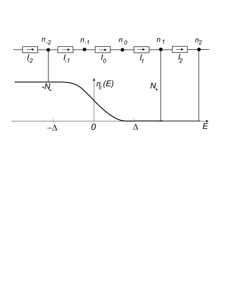
Figure 7.  : Equivalent MAR network in energy space in the limit of negligibly small normal reflection and proximity regions at the NS interfaces.

The MAR network for the present case, in which the contributions of the proximity effect and normal scattering at the interfaces have been neglected, is shown in Fig. 7. Within such model i) the renormalized resistances coincide with the bare ones, ii) the Andreev reflection inside the gap is complete: $R_{A}=0$, $G_{T}=0$ at $|E|<\Delta$, and iii) the over-the-barrier Andreev reflection, as well as the normal reflection, are excluded: $G_{A}=0$, $R_{T}=0$ at $|E|>\Delta$. As the result, the network is essentially simplified and represents a series of Drude resistances connected periodically, at the energies $E_{k}=E+keV$, with the distributed “voltage source” $n_{F}(E)$. The “potentials” $n_{k}$ of the network nodes with even numbers $k$ represent equal electron and hole populations $n^{e,h}_{0}(E_{k})$ at the left NS interface, whereas the potentials of the odd nodes describe equal boundary populations $n^{e,h}_{d}(E_{k}\mp eV)$ at the right interface. The “currents” $I_{k}$ entering $k$-th node are related to the probability currents $n^{\prime}(E_{k})=\partial n(E_{k})/\partial x$ as $I_{k}(E)=-\sigma_{N}n^{e\prime}(E_{k-1})$ (odd $k$) and $I_{k}(E)=\sigma_{N}n^{h\prime}(E_{k})$ (even $k$), and represent partial electric currents transferred by the electrons and holes across the junction, obeying Ohm’s law in energy space, $I_{k}=(n_{k-1}-n_{k})/R_{N}$. Within the gap, $|E_{k}|<\Delta$, i.e., at $-N_{-}<k<N_{+}$, the nodes are disconnected from the reservoir due to complete Andreev reflection and therefore all currents flowing through the subgap nodes are equal.

The analytical equations corresponding to the MAR network are as follows: At $|E|>\Delta$, the boundary populations $n_{0,d}(E)=n(E,x)\left|{}_{x=0,d}\right.$ are local-equilibrium Fermi functions, $n^{e,h}_{0}(E)=n_{F}(E)$, $n^{e,h}_{d}(E)=n_{F}(E\pm eV)$ (we use the potential of the left electrode as the energy reference level). At subgap energies, $|E|<\Delta$, the boundary conditions are modified in accordance with the mechanics of complete Andreev reflection which equalizes the electron and hole population numbers at a given electrochemical potential and blocks the net probability current through the NS interface [7],

$$\displaystyle n^{e}_{0}(E)=n^{h}_{0}(E),\;n^{e}_{d}(E-eV)=n^{h}_{d}(E+eV),$$

$$\displaystyle n^{e\prime}_{0}(E)+n^{h\prime}_{0}(E)=0,\;n^{e\prime}_{d}(E-eV)+n^{h\prime}_{d}(E+eV)=0,$$ (42)

where $n^{\prime}_{0,d}$ are the boundary values of the electron and hole probability flows $\partial n/\partial x$. The recurrences for boundary populations and diffusive flows within the subgap region read

$$n^{e,h}_{0}(E-eV)-n^{e,h}_{0}(E+eV)=\mp 2dn^{e,h\prime}(E\mp eV),$$ (43)

$$n^{e,h\prime}_{0}(E-eV)=n^{e,h\prime}_{0}(E+eV).$$

Due to periodicity of the network, the partial currents obey the relationship $I_{k}(E)=I_{m}(E_{k-m})$, and the boundary population $n_{0}$ is related to the node potentials $n_{k}$ as $n_{0}(E_{k})=n_{k}(E)$. This allows us to reduce the integration over energy in Eqs. (40) and (41) to an elementary interval $0<E<eV$,

$$\displaystyle I={1\over e}\int_{0}^{eV}dE\,J(E),\quad J(E)=\sum_{k=-\infty}^{\infty}I_{k},$$ (44)

$$\displaystyle S={2\over R_{N}}\int_{0}^{eV}dE\sum_{k=-\infty}^{\infty}\left[2n_{k}(1-n_{k})+{1\over 3}(R_{N}I_{k})^{2}\right].$$ (45)

The “potentials” of the nodes outside the gap, $|E_{k}|>\Delta$, are equal to local-equilibrium values of the Fermi function, $n_{k}(E)=n_{F}(E_{k})$ at $k\geq N_{+}$, $k\leq-N_{-}$. The partial currents flowing between these nodes,

$$I_{k}=\left[n_{F}(E_{k-1})-n_{F}(E_{k})\right]/R_{N},\;\;k>N_{+},\;k\leq-N_{-},$$ (46)

are associated with thermally excited quasiparticles. The subgap currents may be calculated by Ohm’s law for the series of $N_{+}+N_{-}$ subgap resistors,

$$I_{k}={n_{-}-n_{+}\over(N_{+}+N_{-})R_{N}},\;\;-N_{-}<k\leq N_{+},$$ (47)

where $n_{\pm}(E)=n_{F}(E_{\pm N_{\pm}})$. From Eqs. (46) and (47) we obtain the current spectral density in Eq. (44) as $J(E)=1/R_{N}$, which results in Ohm’s law, $V=IR_{N}$, for the electric current through the junction. This conclusion is related to our disregarding the proximity effect and the normal scattering at the interface. Actually, both of these factors lead to the appearance of SGS and excess or deficit currents in the $I$-$V$ characteristic, with the magnitude increasing along with the interface barrier strength and the ratio $\xi_{0}/d$ [7].

The subgap populations can be found as the potentials of the nodes of the subgap “voltage divider”,

$$n_{k}=n_{-}-(n_{-}-n_{+}){N_{-}+k\over N_{+}+N_{-}}.$$ (48)

By making use of Eqs. (45)-(48), the net current noise can be expressed through the sum of the thermal noise of quasiparticles outside the gap and the subgap noise, $S=S_{>}+S_{\Delta}$, where

$$S_{>}\!=\!{4T\over 3R_{N}}\!\left\{\!2\left[n_{F}(\Delta)\!+\!n_{F}(\Delta\!+\!eV)\right]\!+\!\!\left[{eV\over T}\!+\!\ln\!{n_{F}(\Delta\!+\!eV)\over n_{F}(\Delta)}\right]\!\coth{eV\over 2T}\right\}\!\!,$$ (49)

and

$$\displaystyle S_{\Delta}={2\over 3R_{N}}\int_{0}^{eV}dE\,(N_{+}+N_{-})\left[f_{+-}+f_{-+}+2(f_{++}+f_{--})\right],$$

$$\displaystyle f_{\alpha\beta}=n_{\alpha}(1-n_{\beta}).$$ (50)

At low temperatures, $T\ll\Delta$, the thermal noise $S_{>}$ vanishes, and the total noise coincides with the subgap shot noise, which takes the form

$$S={2\over 3R_{N}}\int_{0}^{eV}dE\,(N_{+}+N_{-})={2\over 3R_{N}}(eV+2\Delta),$$ (51)

of $1/3$-suppressed Poisson noise $S=(2/3)q^{\it{eff}}I$ for the effective charge $q^{\it{eff}}=e(1+2\Delta/eV)$ [26]. At $V\rightarrow 0$, the shot noise turns to a constant value $4\Delta/3R$. At finite voltages, this quantity plays the role of the “excess” noise, i.e. the voltage-independent addition to the shot noise of a normal metal at low temperatures [see Fig. 8(a)]. Unlike short junctions, where the excess noise is proportional to the excess current [29], in our system the excess current is small and has nothing to do with large excess noise.

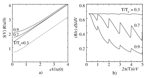
Figure 8.  : Spectral density $S$ of current noise vs voltage (a) and its derivative $dS/dV$ vs inverse voltage (b) at different temperatures. Dashed line shows the result for normal metal junction [10] at $T=0.3T_{c}$.

Results of numerical calculation of the noise at finite temperature are shown in Fig. 8. While the temperature increases, the noise approaches its value for normal metal structures [10], with additional Johnson-Nyquist noise coming from thermal excitations. In this case, the voltage-independent part of current noise may be qualitatively approximated by the Nyquist formula $S(T)=4T^{\ast}/R$ with the effective temperature $T^{\ast}=T+\Delta(T)/3$. The most remarkable phenomenon at nonzero temperature is the appearance of steps in the voltage dependence of the derivative $dS/dV$ at the gap subharmonics $eV=2\Delta/n$ [Fig. 8(b)], which reflect discrete transitions between the quasiparticle trajectories with different numbers of Andreev reflections. The magnitude of SGS decreases both at $T\rightarrow 0$ and $T\rightarrow T_{c}$, which resembles the behavior of SGS in the $I$-$V$ characteristic of long ballistic SNS junction with perfect interfaces within the OTBK model [2, 3]. A small “residual” SGS in current noise, similar to the one in the $I$-$V$ characteristic [7], should occur at $T\rightarrow 0$ due to normal scattering at the interface or due to proximity effect [see comments to Eq. (47)].

3.2 Noise of tunnel barrier

It is instructive to compare the shot noise of a distributed source considered in the previous section with the one produced by a localized scatterer, e.g. opaque tunnel barrier with the resistance $R\gg R_{N}$ inserted in the normal region [25], see Fig. 9. In this case, the potential drops at the tunnel barrier, and the population number is almost constant within the conducting region, while undergoes discontinuity at the barrier. However, the recurrences in Eqs. (3.1), (43) are not sensitive to the details of spatial distribution of the population numbers, and therefore the result of the previous section, Eq. (48), must be also valid for the present case. General equation for the noise in superconducting tunnel junctions has been derived in Ref. [42]. In our case of long SNINS junction, this equation takes the form,

$$S=\int^{+\infty}_{-\infty}{dE\over R}\left[f(E)+f(E+eV)-f(E)f(E+eV)\right],$$ (52)

where $f=n^{e}+n^{h}$. Taking into account the distribution function in Eq. (48), the noise power (52) at zero temperature becomes

$$S\!=\!{2\over R}\int^{-\Delta}_{-\Delta-eV}{dE\over 3}\left[N_{+}+N_{-}+{2\over N_{+}+N_{-}}\right].$$ (53)

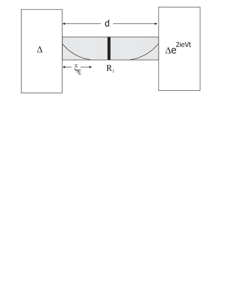
Figure 9.  : Diffusive mesoscopic SNS junction with a tunnel barrier (bold line).

At voltages $eV>2\Delta$ this formula gives conventional Poissonian noise $S=2eI$. At subgap voltages, the noise power undergoes enhancement: it shows a piecewise linear voltage dependence, $dS/dV=(2e/3R)[1+4/(\,\mbox{Int}\,(2\Delta/eV)+2)]$, with kinks at the subharmonics of the superconducting gap, $eV_{n}=2\Delta/n$ (see Fig. 10). At zero voltage, the noise power approaches the constant value $S(0)=4\Delta/3R$, coinciding with the noise power of the diffusive normal region without tunnel barrier. However, in contrast to the latter case, the voltage dependence of the noise here exhibits SGS already at zero temperature, which consists of a step-wise increase of the effective charge $q^{\it{eff}}(V)=S(V)/2I$ with decreasing voltage,

$${q^{\it{eff}}(n)\over e}={1\over 3}\left(n+1+{2\over n+1}\right)=1,{11\over 9},{22\over 15},\dots$$ (54)

At $eV\rightarrow 0$ the effective charge increases as $q^{\it{eff}}(V)/e\approx(1/3)(1+2\Delta/eV)$.

Calculation presented in this section shows that the $1/3$-factor in the expression for the noise has no direct relation to the Fano factor for diffusive normal conductors but is a general property of the incoherent MAR regime. Appearance of this factor results from the infinitely increasing chain of the normal resistances in the MAR network at small voltage, in close analogy with the case of multibarrier tunnel structures considered in Ref. [9].

Figure 10.  : Spectral density $S(V)$ of current shot noise and effective transferred charge $q(V)$ as functions of applied voltage $V$. In the absence of inelastic collisions (solid lines), the shot noise power approaches the finite value $S(0)=4\Delta/3R$ at $eV\rightarrow 0$, and the effective charge increases as $q(V)=(e/3)(1+2\Delta/eV)$. The effect of inelastic scattering is represented by dashed lines for the nonequilibrium parameter $W_{\varepsilon}=5$. The dependence $S(V)$ contains kinks at the gap subharmonics, $eV=2\Delta/n$, as shown in the inset.

4 Effect of inelastic relaxation on MAR

During the previous discussion, an inelastic electron relaxation within the normal region of the contact has been entirely ignored. This is legitimate when inelastic mean free path exceeds the junction length, $l_{\varepsilon}=\sqrt{{\cal D}\tau_{\varepsilon}}\gg d$, or, equivalently, when the inelastic relaxation time exceeds the diffusion time, $\tau_{\varepsilon}\gg\hbar/E_{\it Th}$. In the opposite limiting case, $\tau_{\varepsilon}\ll\hbar/E_{\it Th}$, the energy relaxation completely destroys the MAR regime because the quasiparticle distribution within the normal region becomes equilibrium, and the SNS junction becomes equivalent to the two NS junctions connected in series through the equilibrium normal reservoir. Thus the appearance of the MAR regime is controlled by parameter $W_{\varepsilon}=E_{\it Th}\tau_{\varepsilon}/\hbar$. The relaxation time in these estimates must be considered for the energy of order $\Delta$, $\tau_{\varepsilon}(\Delta)$, since non-equilibrium electron population under the MAR regime develops within the whole subgap energy interval. However, to build up such a nonequilibrium population at small voltage, a long time, $\tau_{\it dwell}=(\hbar/E_{Th})(2\Delta/eV)^{2}$, is actually needed, which exceeds the diffusion time $\hbar/E_{\it Th}$ by squared number of Andreev reflections (see below Eq. (57) and further text). Thus, the condition for the MAR regime, $\tau_{\varepsilon}>\tau_{\it dwell}$, is more restrictive than $W_{\varepsilon}>1$, and in the limit of zero voltage the MAR regime is always suppressed. Hence the effect of the shot noise enhancement disappears at small voltage, and the noise approaches the thermal noise level, the noise temperature being equal to the physical temperature $T$ if the inelastic scattering is dominated by electron-phonon interaction (assuming that the phonons are in equilibrium with the electron reservoir). If the electron-electron scattering dominates, the noise temperature may exceed the temperature $T$ of the electron reservoir if this temperature is small, $T\ll\Delta$ (hot electron regime). The reason is that at low temperature, the subgap electrons are well decoupled from the reservoir (electrons outside the gap) due to weak energy flow through the gap edges. In the cross over region of a small applied voltage, the non-equilibrium electron population appears as the result of the two competing mechanisms: the spectral flow upward in energy space driven by MAR and spectral counter flow due to inelastic relaxation. In this section we briefly consider the behavior of the shot noise in this situation.

To include the inelastic relaxation into the consideration we add the inelastic collision term $I_{\varepsilon}$ to the diffusion equation (9),

$${\cal D}{\partial^{2}n\over\partial x^{2}}=I_{\varepsilon}(n).$$ (55)

At small voltage, $eV\ll\Delta$, the spatial variation of the population number is small, and the function $n(x)$ in the collision term can be replaced by the boundary values, $n_{0}^{e,h}(E)\approx n_{d}^{e,h}(E)\equiv n(E)$. Then including the collision term into the recurrences, Eq. (43), and combining them with equations (3.1), we arrive at the generalized recurrence,

$${\cal D}\left[n(E+2eV)+n(E-2eV)-2n(E)\right]=4I_{\varepsilon}[n(E)].$$ (56)

Within the same approximation, this recurrence is to be considered as differential relation, which results in the diffusion equation for $n(E)$,

$$D_{E}{\partial^{2}n\over\partial E^{2}}=I_{\varepsilon}(n),$$ (57)

where $D_{E}=(eV)^{2}E_{{Th}}/\hbar$ is the diffusion coefficient in energy space.

To demonstrate the effect of electron-phonon scattering and suppression of the current shot noise, it is sufficient to assume the relaxation time approximation in the collision term, $I_{\varepsilon}(n)=(1/\tau_{\varepsilon})[n-n_{F}(T)]$. The results of numerical calculations within this approximation of the shot noise at zero reservoir temperature are presented in Fig. 10 by dashed curves. The rapid decrease of $S(V)$ at low voltage is described by the following analytical approximation,

$$S(V)=S(0){3\over\alpha}\left(\tanh{\alpha\over 2}+{\alpha-\sinh\alpha\over\sinh^{2}\alpha}\right),\quad\alpha={\Delta\over eV\sqrt{W_{\varepsilon}}},$$ (58)

and it occurs when the length of the MAR path in energy space interrupted by inelastic scattering, $eV\sqrt{W_{\varepsilon}}$, becomes smaller than $2\Delta$.

4.1 Hot electron regime

In the case of dominant electron-electron scattering, equation (57) describes the crossover from the “collisionless” MAR regime to the hot electron regime as function of the parameter $D_{E}\tau_{ee}(\Delta)/\Delta^{2}$. In the hot electron limit, $\Delta^{2}\gg D_{E}\tau_{ee}$, the collision integral dominates in Eq. (57), and therefore the approximate solution of the diffusion equation is the Fermi function with a certain effective temperature $T_{0}\ll\Delta$. The value of $T_{0}$ can be found from Eq. (57) integrated over energy within the interval $(-\Delta,\Delta)$ with the weight $E$, taking into account the boundary conditions $n(\pm\Delta)=n_{F}(\pm\Delta/T)$ and the conservation of energy by the collision integral,

$$D_{E}\left[1-2\left(e^{-\Delta/T}+{\Delta\over T_{0}}e^{-\Delta/T_{0}}\right)\right]+2\int_{\Delta}^{\infty}dE\,E\,I_{\varepsilon}=0.$$ (59)

At zero temperature of the reservoir and $T_{0}\ll\Delta$, Eq. (59) takes the form

$$D_{E}\tau_{\it ee}\Delta^{2}=2\int_{\Delta}^{\infty}dE\,E\int_{E-2\Delta}^{\infty}dE^{\prime}\int_{E-E^{\prime}-\Delta}^{\infty}d\omega\,n_{F}(E-E^{\prime}-\omega)n_{F}(E^{\prime})n_{F}(\omega),$$ (60)

and can be reduced to an asymptotic equation for $T_{0}$,

$$(eV)^{2}W_{\varepsilon}\exp(\Delta/T_{0})=T_{0}\Delta(1+T_{0}/\Delta),$$ (61)

which shows that the effective temperature of the subgap electrons decreases logarithmically with decreasing voltage. The noise of the hot subgap electrons is given by the Nyquist formula with temperature $T_{0}$,

$$S(V)=(4T_{0}/R)\left[1-2\exp(-\Delta/T_{0})\right],$$ (62)

where the last term is due to the finite energy interval available for the hot electrons, $|E|<\Delta$. Equations (61), (62) give a reasonably good approximation to the result of the numerical solution of Eq. (57) [27].

5 Summary

We have presented a theory for the current shot noise in long diffusive SNS structures with low-resistive interfaces at arbitrary temperatures. In such structures, the noise is mostly generated by normal electron scattering in the N-region. Whereas the $I$-$V$ characteristics are approximately described by Ohm’s law, the current noise reveals all characteristic features of the MAR regime: “giant” enhancement at low voltages, pronounced SGS, and excess noise at large voltages. The most spectacular feature of the noise in the incoherent MAR regime is a universal finite noise level at zero voltage and at zero temperature, $S=4\Delta/3R$. This effect can be understood as the result of the enhancement of the effective charge of the carriers, $q^{\it eff}=2\Delta/V$, or, alternatively, as the effect of strongly non-equilibrium quasiparticle population in the energy gap region with the effective temperature $T_{0}=\Delta/3$. Appearance of the excess noise is controlled by a large value of the parameter $\tau_{\varepsilon}/\tau_{\it dwell}\gg 1$, where $\tau_{\varepsilon}$ is the inelastic relaxation time, and $\tau_{\it dwell}$ is the time spent by quasiparticle in the contact. At small applied voltage this condition is always violated, and the excess noise disappears. Under the condition of dominant electron-electron scattering, the junction undergoes crossover to the hot electron regime, with the effective temperature of the subgap electrons decreasing logarithmically with the voltage. Calculation of the noise power has been done on the basis of circuit theory of the incoherent MAR [7], which may be considered as an extension of Nazarov’s circuit theory [43] to a system of voltage biased superconducting terminals connected by normal wires in the absence of supercurrent. The theory is valid as soon as the applied voltage is much larger than the Thouless energy: in this case, the overlap of the proximity regions near the NS interfaces is negligibly small, and the ac Josephson effect is suppressed.

References

- [1] Schrieffer, J.R., and Wilkins, J.W. (1963) Two-particle tunneling processes between superconductors, Phys. Rev. Lett., Vol. no. 10, pp. 17-19.
- [2] Klapwijk, T.M., Blonder, G.E., and Tinkham, M. (1982) Explanation of subharmonic energy gap structure in superconducting contacts, Physica B+C, Vol. no. 109-110, pp. 1657-1664.
- [3] Octavio, M., Tinkham, M., Blonder, G.E., and Klapwijk, T.M. (1988) Subharmonic energy-gap structure in superconducting constrictions, Phys. Rev. B, Vol. no. 27, pp. 6739-6746; Flensberg, K., Bindslev Hansen, J., and Octavio, M. (1988) Subharmonic energy-gap structure in superconducting weak links, ibid., Vol. no. 38, pp. 8707-8711.
- [4] Bratus’, E.N., Shumeiko, V.S., and Wendin, G. (1995) Theory of subharmonic gap structure in superconducting mesoscopic tunnel contacts, Phys. Rev. Lett., Vol. no. 74, pp. 2110-2113; Averin, D., and Bardas, A. (1995) ac Josephson effect in a single quantum channel, ibid., Vol. no. 75, pp. 1831-1834; Cuevas, J.C., Martín-Rodero, A., and Levy Yeyati, A. (1996) Hamiltonian approach to the transport properties of superconducting quantum point contacts, Phys. Rev. B , Vol. no. 54, pp. 7366-7379.
- [5] Bardas, A., and Averin, D.V. (1997) Electron transport in mesoscopic disordered superconductor-normal-metal-superconductor junctions, Phys. Rev. B, Vol. no. 56, pp. 8518-8521; Zaitsev, A.V., and Averin, D.V. (1998) Theory of ac Josephson effect in superconducting constrictions, Phys. Rev. Lett., Vol. no. 80, pp. 3602-3605.
- [6] Zaitsev, A.V., (1990) Properties of ”dirty” S-S’-N and S-S’-S structures with potential barriers at the metal boundaries, JETP Lett., Vol. no. 51, pp. 41-46.
- [7] Bezuglyi, E.V., Bratus’, E.N., Shumeiko, V.S., Wendin, G., and Takayanagi, H. (2000) Circuit theory of multiple Andreev reflections in diffusive SNS junctions: The incoherent case, Phys. Rev. B, Vol. no. 62, pp. 14439-14451.
- [8] Blanter, Ya.M., and Büttiker, M. (2000) Shot noise in mesoscopic conductors, Physics Reports, Vol. no. 336, pp. 1-166.
- [9] de Jong, M.J.M., and Beenakker, C.W.J. (1996) Semiclassical theory of shot noise in mesoscopic conductors, Physica A, Vol. no. 230, pp. 219-249.
- [10] Nagaev, K.E. (1992) On the shot noise in dirty metal contacts, Phys. Lett. A, Vol. no. 169, pp. 103-107.
- [11] Beenakker, C.W.J., and Büttiker, M. (1992) Suppression of shot noise in metallic diffusive conductors, Phys. Rev. B Vol. no. 46, pp. 1889-1892; González, T., González, C., Mateos, J., Pardo, D., Reggiani, L., Bulashenko, O.M., and Rubí, J.M. (1998) Universality of the 1/3 shot noise suppression factor in nondegenerate diffusive conductors, Phys. Rev. Lett., Vol. no. 80, pp. 2901-2904; Sukhorukov, E.V., and Loss, D. (1998) Universality of shot noise in multiterminal diffusive conductors, ibid., Vol. no. 80, pp. 4959-4962.
- [12] Schoelkopf, R.J., Burke, P.J., Kozhevnikov, A.A., Prober, D.E., and Rooks, M. J. (1997) Frequency dependence of shot noise in a diffusive mesoscopic conductor, Phys. Rev. Lett., Vol. no. 78, pp. 3370-3373; Henny, M., Oberholzer, S., Strunk, C., and Schönenberger, C. (1999) 1/3-shot-noise suppression in diffusive nanowires, Phys. Rev. B, Vol. no. 59, pp. 2871-2880.
- [13] Nagaev, K.E. (1995) Influence of electron-electron scattering on shot noise in diffusive contacts, Phys. Rev. B, Vol. no. 52, pp. 4740-4743; (1998) Frequency-dependent shot noise as a probe of electron-electron interaction in mesoscopic diffusive contacts, ibid., Vol. no. 58, pp. 7512-7515; Naveh, Y., Averin, D.V., and Likharev, K.K. (1998) Shot noise in diffusive conductors: A quantitative analysis of electron-phonon interaction effects, ibid., Vol. no. 58, pp. 15371-15374; Naveh, Y., Averin, D.V., and Likharev, K.K. (1999) Noise properties and ac conductance of mesoscopic diffusive conductors with screening, ibid., Vol. no. 59, pp. 2848-2860.
- [14] Liefrink, F., Dijkhuis, J.I., de Jong, M.J.M., Molenkamp, L.W., and van Houten, H. (1994) Experimental study of reduced shot noise in a diffusive mesoscopic conductor, Phys. Rev. B, Vol. no 49, pp. 14066-14069; Steinbach, A.H., Martinis, J.M., and Devoret, M.H. (1996) Observation of hot-electron shot noise in a metallic resistor, Phys. Rev. Lett., Vol. no. 76, pp. 3806-3809.
- [15] Khlus, V.A. (1987) Current and voltage fluctuations in microjunctions between normal metals and superconductors, Sov. Phys. JETP, Vol. no. 66, pp. 1243-1249; Muzykantskii, B.A., and Khmelnitskii, D.E. (1994) On quantum shot noise, Physica B, Vol. no. 203, pp. 233-239; de Jong, M.J.M., and Beenakker, C.W.J. (1994) Doubled shot noise in disordered normal-metal-superconductor junctions, Phys. Rev. B, Vol. no. 49, pp. 16070-16073.
- [16] Jehl, X., Payet-Burin, P., Baraduc, C., Calemczuk, R., and Sanquer, M. (1999) Andreev reflection enhanced shot noise in mesoscopic SNS junctions, Phys. Rev. Lett., Vol. no. 83, pp. 1660-1663; Kozhevnikov, A.A., Schoelkopf, R.J., and Prober, D.E. (2000) Observation of photon-assisted noise in a diffusive normal metal-superconductor junction, ibid., Vol. no. 84, pp. 3398-3401.
- [17] Belzig, W., and Nazarov, Yu.V. (2001) Full counting statistics in diffusive normal-superconducting structures, Phys. Rev. Lett., Vol. no. 87, 197006.
- [18] Hessling, J.P. (1996) Fluctuations in mesoscopic constrictions, PhD Thesis, Göteborg.
- [19] Naveh, Y., and Averin, D.V. (1999) Nonequilibrium current noise in mesoscopic disordered superconductor-normal-metal-superconductor junctions, Phys. Rev. Lett., Vol. no. 82, pp. 4090-4093.
- [20] Cuevas, J.C., Martín-Rodero, A., and Levy Yeyati, A. (1999) Shot noise and coherent multiple charge transfer in superconducting quantum point contacts, Phys. Rev. Lett., Vol. no. 82, pp. 4086-4089.
- [21] Dieleman, P., Bukkems, H.G., Klapwijk, T.M., Schicke, M., and Gundlach, K.H. (1997) Observation of Andreev reflection enhanced shot noise, Phys. Rev. Lett., Vol. no. 79, pp. 3486-3489.
- [22] Cron R., Goffman M.F., Esteve D., and Urbina C. (2001) Multiple-charge-quanta shot noise in superconducting atomic contacts, Phys. Rev. Lett., Vol. no. 86, pp. 4104-4107.
- [23] Hoss, T., Strunk, C., Nussbaumer, T., Huber, R., Staufer, U., and Schönenberger, C. (2000) Multiple Andreev reflection and giant excess noise in diffusive superconductor/normal-metal/superconductor junctions, Phys. Rev. B, Vol. no. 62, pp. 4079-4085.
- [24] Strunk, C. and Sch nenberger C. (2002) Shot noise in diffusive superconductor/normal metal heterostructures, This volume.
- [25] Bezuglyi, E.V., Bratus’, E.N., Shumeiko, V.S., and Wendin, G. (1999) Multiple Andreev reflections and enhanced shot noise in diffusive superconducting-normal-superconducting junctions, Phys. Rev. Lett., Vol. no. 83, pp 2050-2053.
- [26] Bezuglyi, E.V., Bratus’, E.N., Shumeiko, V.S., and Wendin, G. (2001) Current noise in long diffusive SNS junctions in the incoherent multiple Andreev reflections regime, Phys. Rev. B, Vol. no. 63, 100501.
- [27] Nagaev, K.E. (2001) Frequency-dependent shot noise in long disordered superconductor–normal-metal–superconductor contacts, Phys. Rev. Lett., Vol. no. 86, pp. 3112-3115.
- [28] Hoffmann C., Lefloch F., and Sanquer M., (2002) Inelastic relaxation and noise temperature in S/N/S junctions, Preprint.
- [29] Hessling, J.P., Shumeiko, V.S., Galperin, Yu.M., and Wendin, G. (1996) Current noise in biased superconducting weak links, Europhys. Lett., Vol. no. 34, pp. 49-54.
- [30] Larkin, A.I., and Ovchinnikov, Yu.N. (1975) Nonlinear conductance of superconductors in the mixed state, Sov. Phys. JETP, Vol. no. 41, pp. 960-965; (1977) Nonlinear effects during motion of vortices in superconductors, ibid., Vol. no. 46, pp. 155-162.
- [31] Kupriyanov, M.Yu., and Lukichev, V.F. (1988) Influence of boundary transparency on the critical current of “dirty” SS’S structures, Sov. Phys. JETP, Vol. no. 67, pp. 1163-1168.
- [32] Blonder, G.E., Tinkham, M., and Klapwijk, T.M. (1982) Transition from metallic to tunneling regimes in superconducting microconstrictions: Excess current, charge imbalance, and supercurrent conversion, Phys. Rev. B, Vol. no. 25, pp. 4515-4532.
- [33] Lambert, C.J., Raimondi, R., Sweeney, V., and Volkov, A.F. (1997) Boundary conditions for quasiclassical equations in the theory of superconductivity, Phys. Rev. B, Vol. no 55, pp. 6015-6021.
- [34] Zaikin, A.D., and Zharkov, G.F. (1981) Theory of wide dirty SNS junctions, Sov. J. Low Temp. Phys., Vol. no. 7, pp. 375-379.
- [35] Bezuglyi, E.V., Bratus’, E.N., and Galaiko, V.P. (1999) On the theory of Josephson effect in a diffusive tunnel junction, Low Temp. Phys., Vol. no. 25, pp 167-174.
- [36] Artemenko, S.N., Volkov, A.F., and Zaitsev, A.V. (1979) Theory of nonstationary Josephson effect in short superconducting contacts, Sov. Phys. JETP, Vol. no. 49, pp. 924-931.
- [37] Volkov, A.F., and Klapwijk, T.M. (1992) Microscopic theory of superconducting contacts with insulating barriers, Phys. Lett. A, Vol. no. 168, pp. 217-224.
- [38] Volkov, A.F., Zaitsev, A.V., and Klapwijk, T.M. (1993) Proximity effect under nonequilibrium conditions in double-barrier superconducting junctions, Physica C, Vol. no. 210, pp. 21-34.
- [39] Nazarov, Yu.V., and Stoof, T.H. (1996) Diffusive conductors as Andreev interferometers, Phys. Rev. Lett., Vol. no. 76, pp. 823-826; Stoof, T.H., and Nazarov, Yu.V. (1996) Kinetic-equation approach to diffusive superconducting hybrid devices, Phys. Rev. B, Vol. no. 53, pp. 14496-14505; Volkov, A.F., Allsopp, N., and Lambert, C.J. (1996) Crossover from mesoscopic to classical proximity effects induced by particle-hole symmetry breaking in Andreev interferometers, J. Phys.: Cond. Matter, Vol. no. 8, pp. L45-L50.
- [40] Kogan, Sh.M., and Shul’man, A.Ya. (1969) Theory of fluctuations in a nonequilibrium electron gas, Sov. Phys. JETP, Vol. no. 29, pp. 467-474; Nagaev, K.E. (1998) Long-range Coulomb interaction and frequency dependence of shot noise in mesoscopic diffusive contacts, Phys. Rev. B, Vol. no. 57, pp. 4628-4634.
- [41] Nagaev, K.E., and Büttiker, M. (2001) Semiclassical theory of the shot noise in disordered SN contacts, Phys. Rev. B, Vol. no 63, 081301.
- [42] Larkin, A.I., and Ovchinnikov, Yu.N. (1984) Current damping in superconducting junctions with nonequilibrium electron distribution functions, Sov. Phys. JETP, Vol. no. 60, pp. 1060-1067.
- [43] Nazarov, Yu.V. (1994) Circuit theory of Andreev conductance, Phys. Rev. Lett., Vol. no. 73, pp. 1420-1423; (1999) Novel circuit theory of Andreev reflection, Superlattices Microstruct., Vol. no. 25, pp. 1221-1231.