Weak Convergence of a Seasonally Forced Stochastic Epidemic Model

Abstract

In this study we extend the results of Kurtz (1970,1971) to show the weak convergence of epidemic processes that include explicit time dependence, specifically where the transmission parameter, $\beta(t)$, carries a time dependency. We first show that when population size goes to infinity, the time inhomogeneous process converges weakly to the solution of the mean-field ODE. Our second result is that, under proper scaling, the central limit type fluctuations converge to a diffusion process.

1 Introduction

Much of mathematical epidemiology draws upon deterministic descriptions of disease transmission processes [1]. Deterministic models are attractive, in part, because they are easy to analyze and simulate. The importance of stochastic effects on disease transmission processes has, however, long been appreciated [2, 3, 13] and so it is natural to ask about the relationship between stochastic and deterministic models of a given process.

Kurtz [14] showed, for a general class of population models, weak convergence of the stochastic model to the corresponding deterministic model as the system size, $N$, tends to infinity. Further, in [15] Kurtz provided a central limit theorem-type result that explored the nature of this convergence in more detail, revealing a diffusion process behavior. These limiting results have been used to justify the use of the multivariate normal approximation introduced by [17] to close moment equations for nonlinear population models. Use of this approach (e.g. [12, 10]) allows one to assess the magnitude of stochastic fluctuations likely to be seen about the deterministic solution and hence determine the adequacy of a deterministic description.

Many epidemic processes, however, have an explicit time dependence [9]. For instance, an infectious agent may be more transmissible at certain times of the year than at others. Several biological and social mechanisms can give rise to such seasonality, including sensitivity of certain viruses to humidity and congregation of children during school sessions.

In this study, we extend the results of Kurtz to epidemic processes that include explicit time dependence, specifically where the transmission parameter, $\beta(t)$, carries a time dependency. The paper is organized as follows: in Section 2 we introduce the model. Section 3 provides a weak convergence result and in Section 4 a central limit theorem-type result is given. Simulation results are shown in Section 5.

2 The Model

We consider the seasonal SIR (susceptible/infective/recovered) model taking value $(S^{N}(t),I^{N}(t),R^{N}(t))\in(\mathbb{Z}^{+}\cup\{0\})^{3}$ with transition rates as follows:

Event	Transition	Rate at which event occurs
Birth	$S\rightarrow S+1$	$\nu(S+I+R)$
Susceptible Death	$S\rightarrow S-1$	$\nu S$
Infection	$S\rightarrow S-1,\ I\rightarrow I+1$	$\beta(t)SI/(S+I+R)$
Recovery	$I\rightarrow I-1,\ R\to R+1$	$\gamma I$
Infectious Death	$I\rightarrow I-1$	$\nu I$
Recovered Death	$R\rightarrow R-1$	$\nu R$

Table 1: Transition rates for the seasonal SIR model

Here, $\nu$ denotes the per capita birth and death rate, which we assume to be equal. $\gamma$ denotes the per capita recovery rate, implying that the average duration of infection is $1/\gamma$. $N$ is equal to the initial population size, $N=S(0)+I(0)+R(0)$, although, as discussed further below, it should be noted that the population size is not constant for this model, despite having equal per capita demographic parameters.

The transmission parameter, $\beta(t)$ is assumed to be a periodic function with period one. For definiteness, we take the following sinusoidal form: $\beta(t)=\beta_{0}[1+\beta_{1}\cos(2\pi t)]$, where $\beta_{0}>0$ and $\beta_{1}\in(0,1)$. It should be noted, however, that our results apply to a much broader class of functions.

From the transition rates above, it is easy to see that the stochastic model above is associated with the following mean-field ODE:

$$\frac{dx_{t}}{dt}=F_{1}(x_{t},y_{t},z_{t},t)=\nu(y_{t}+z_{t})-\beta(t)x_{t}y_{t}$$ (1)

$$\frac{dy_{t}}{dt}=F_{2}(x_{t},y_{t},z_{t},t)=\beta(t)x_{t}y_{t}-(\nu+\gamma)y_{t}$$

$$\frac{dz_{t}}{dt}=F_{3}(x_{t},y_{t},z_{t},t)=\gamma y_{t}-\nu z_{t}.$$

where $x_{t}$, $y_{t}$ and $z_{t}$ now represent the fractions of the population in each state.

3 Weak Convergence to the Solution of ODE

We first prove the following weak convergence result:

Theorem 1.

Let $T^{N}(s)=S^{N}(s)+I^{N}(s)+R^{N}(s)$. For any $t<\infty$, as $N\rightarrow\infty$, the stochastic model

$$\left(\frac{S^{N}(s)}{T^{N}(s)},\frac{I^{N}(s)}{T^{N}(s)},\frac{R^{N}(s)}{T^{N}(s)}\right)$$

with initial values

$$\left(\frac{S^{N}(0)}{N},\frac{I^{N}(0)}{N},\frac{R^{N}(0)}{N}\right)\rightarrow(x_{0},y_{0},z_{0})$$ (2)

converges weakly to $(x_{s},y_{s},z_{s})$ the solution of the mean-field ODE equation (1) in $[0,t]$ with initial values $(x_{0},y_{0},z_{0})$.

Proof.

To show the weak convergence we will first use the idea of graphical representation as in [6] to construct the inhomogenous Markov process $(S^{N}(t),I^{N}(t),R^{N}(t))$ from the following family of independent Poisson processes and i.i.d. uniform random variables.

[Remark]: At this point, the graphical representation may seem unnecessary in defining in the process. But the reason we want to use the technique is to allow us to couple the original system and its “truncated” version (see Table 2 for details) in the same space, and keep them coinciding with each other for a long time. So here we strongly recommend the reader to compare the construction below with the one for the truncated process, to see how we can construct the two systems in the same probability space using the same family of Poisson processes and random variables.

The construction is as follows:

• For all $x\in\mathbb{Z}^{+}$ define a family of independent Poisson processes at rate $\nu$, denoted by $\{B_{n}^{x}:x\in\mathbb{Z}^{+},n\geq 1\}$. At each space time point $(x,B_{n}^{x})$, i.e., the $n$th jumping time of the Poisson process associate with point $x$, we have $S^{N}=S^{N}+1$ if and only if $T^{N}(B_{n}^{x}-)=S^{N}(B_{n}^{x}-)+I^{N}(B_{n}^{x}-)+R^{N}(B_{n}^{x}-)\geq x$.

• For all $x\in\mathbb{Z}^{+}$ define a family of independent Poisson processes at rate $\nu$, denoted by $\{DS_{n}^{x}:x\in\mathbb{Z}^{+},n\geq 1\}$ ,which are also independent to $\{B_{n}^{x}\}$. At each space time point $(x,DS_{n}^{x})$, we have $S^{N}=S^{N}-1$ if and only if $S^{N}(DS_{n}^{x}-)\geq x$.

• For all $x\in\mathbb{Z}^{+}$ define a family of independent Poisson processes at rate $\nu$, denoted by $\{DI_{n}^{x}:x\in\mathbb{Z}^{+},n\geq 1\}$ which are also independent to processes defined above. At each space time point $(x,DI_{n}^{x})$, we have $I^{N}=I^{N}-1$ if and only if $I^{N}(DI_{n}^{x}-)\geq x$.

• For all $x\in\mathbb{Z}^{+}$ define a family of independent Poisson processes at rate $\nu$, denoted by $\{DR_{n}^{x}:x\in\mathbb{Z}^{+},n\geq 1\}$ which are also independent to processes defined above. At each space time point $(x,DR_{n}^{x})$, we have $R^{N}=R^{N}-1$ if and only if $I^{N}(DR_{n}^{x}-)\geq x$.

• For all $x\in\mathbb{Z}^{+}$ define a family of independent Poisson processes at rate $\gamma$, denoted by $\{RI_{n}^{x}:x\in\mathbb{Z}^{+},n\geq 1\}$ which are also independent to processes defined above. At each space time point $(x,RI_{n}^{x})$, we have $I^{N}=I^{N}-1$ and $R^{N}=R^{N}+1$ if and only if $I^{N}(RI_{n}^{x}-)\geq x$.

• For all $x\in\mathbb{Z}^{+}$ define a family of independent Poisson processes at rate $\beta_{0}(1+\beta_{1})$, denoted by $\{IN_{n}^{x}:x\in\mathbb{Z}^{+},n\geq 1\}$, which are also independent to processes defined above. Moreover, define a family of i.i.d. random variables $\{U_{n}^{x}\sim U(0,1):x\in Z^{+},n\geq 1\}$ which are also independent to processes defined above. At each space-time point $[x,IN_{n}^{x}]$, we have $S^{N}=S^{N}-1,I^{N}=I^{N}+1$ if and only if that $S^{N}(IN_{n}^{x}-)\geq x$ and

  $$U_{n}^{x}\leq\frac{\beta(IN_{n}^{x})I^{N}(IN_{n}^{x}-)}{\beta_{0}(1+\beta_{1})T^{N}(IN_{n}^{x}-)}.$$

To show the construction above is well defined and is actually the seasonal SIR model we want, we first refer to [6] to show the process never explodes. To show this, consider a monotone increasing process $M_{t}$ defined as follows:

• At each space time point $(x,B_{n}^{x})$, $M_{t}=M_{B_{n}^{x}-}+1$ if and only if $M_{B_{n}^{x}-}\geq x$.

Then by definition it is easy to see that $M_{t}\geq S^{N}(t)+I^{N}(t)+R^{N}(t)$ for all $t\geq 0$. Noting that for all $k$,

$$\sum_{i=k}^{\infty}\frac{1}{i}=\infty,$$

so the bigger process $M_{t}$ never explodes. This implies at each time $t$, all the jumps in our system must be in the following finite family of Poisson processes: $\{B_{n}^{x}\}_{x=1}^{M_{t}},\{DS_{n}^{x}\}_{x=1}^{M_{t}},\{DI_{n}^{x}\}_{x=1}^{M_{t}},\{DR_{n}^{x}\}_{x=1}^{M_{t}},\{RI_{n}^{x}\}_{x=1}^{M_{t}}$, and $\{I_{n}^{x}\}_{x=1}^{M_{t}}$. Note that a Poisson processes (with probability one) has only finite jumps in a finite time interval, it is straightforward to verify that the process we defined above never explodes. Then for each time $t$, one can easily check the transition rates given the current value of $(S,I,R)$ in the process we construct in the bullet list above. According to the Kolmogorov forward equation and Theorem 1 about Poisson thinning in [11], it is easy to see that the process defined by the devices above has the same transition rates as in Table 1. Thus the process defined above is exactly the stochastic seasonal SIR model $(S^{N}(t),I^{N}(t),R^{N}(t))$ that we want.

Note that, because the population size is unbounded, the transition rates of the system above can possibly (but not likely) go large. Our next step is to introduce a truncated version of the seasonal SIR model. Consider $(\hat{S}^{N}(t),\hat{I}^{N}(t),\hat{R}^{N}(t))$ to be the truncated version with new transition rates as follows:

Event	Transition	Rate at which event occurs
Birth	$\hat{S}\rightarrow\hat{S}+1$	$\nu[(\hat{S}+\hat{I}+\hat{R})\wedge 2N]$
Susceptible Death	$\hat{S}\rightarrow\hat{S}-1$	$\nu(\hat{S}\wedge 2N)$
Infection	$\hat{S}\rightarrow\hat{S}-1,\ \hat{I}\rightarrow\hat{I}+1$	$\beta(t)(\hat{S}\wedge 2N)\hat{I}/(\hat{S}+\hat{I}+\hat{R})$
Recovery	$\hat{I}\rightarrow\hat{I}-1,\ \hat{R}\to\hat{R}+1$	$\gamma(\hat{I}\wedge 2N)$
Infectious Death	$\hat{I}\rightarrow\hat{I}-1$	$\nu(\hat{I}\wedge 2N)$
Recovered Death	$\hat{R}\rightarrow\hat{R}-1$	$\nu(\hat{R}\wedge 2N)$

Table 2: Transition rates for the truncated model

Here, $a\wedge b=\min(a,b)$.

By definition, the transition rate of $(\hat{S}^{N}(t),\hat{I}^{N}(t),\hat{R}^{N}(t))$ is no larger than

$$MN=\max\{2\nu N,2\beta_{0}(1+\beta_{1})N,2\gamma N\}$$

and thus is bounded. Moreover, using the same family of Poisson processes and uniform random variables in the bullet list above, we can construct a copy of the truncated process as follows:

• At each space time point $(x,B_{n}^{x})$, we have $\hat{S}^{N}=\hat{S}^{N}+1$ if and only if $\hat{T}^{N}(B_{n}^{x}-)=\hat{S}^{N}(B_{n}^{x}-)+\hat{I}^{N}(B_{n}^{x}-)+\hat{R}^{N}(B_{n}^{x}-)\geq x$ and $x\leq 2N$.

• At each space time point $(x,DS_{n}^{x})$, we have $\hat{S}^{N}=\hat{S}^{N}-1$ if and only if $\hat{S}^{N}(DS_{n}^{x}-)\geq x$ and $x\leq 2N$.

• At each space time point $(x,DI_{n}^{x})$, we have $\hat{I}^{N}=\hat{I}^{N}-1$ if and only if $\hat{I}^{N}(DI_{n}^{x}-)\geq x$ and $x\leq 2N$.

• At each space time point $(x,DR_{n}^{x})$, we have $\hat{R}^{N}=\hat{R}^{N}-1$ if and only if $\hat{R}^{N}(DR_{n}^{x}-)\geq x$ and $x\leq 2N$.

• At each space time point $(x,RI_{n}^{x})$, we have $\hat{I}^{N}=\hat{I}^{N}-1$ and $\hat{R}^{N}=\hat{R}^{N}+1$ if and only if $\hat{I}^{N}(RI_{n}^{x}-)\geq x$ and $x\leq 2N$.

• At each space-time point $[x,IN_{n}^{x}]$, we have $\hat{S}^{N}=\hat{S}^{N}-1,\hat{I}^{N}=\hat{I}^{N}+1$ if and only if that $\hat{S}^{N}(IN_{n}^{x}-)\geq x$, $x\leq 2N$ and

  $$U_{n}^{x}\leq\frac{\beta(IN_{n}^{x})\hat{I}^{N}(IN_{n}^{x}-)}{\beta_{0}(1+\beta_{1})\hat{T}^{N}(IN_{n}^{x}-)}.$$

From the gadgets as above, it is easy to check that we defined the truncated process $(\hat{S}^{N}(t),\hat{I}^{N}(t),\hat{R}^{N}(t))$ in the same probability space as the original process $(S^{N}(t),I^{N}(t),R^{N}(t))$. Moreover, consider the stopping time

$$\tau_{N}=\inf\{t:T^{N}(t)>2N\}.$$ (3)

Then by definition we immediately have

Proposition 1.

$(\hat{S}^{N}(t),\hat{I}^{N}(t),\hat{R}^{N}(t))\equiv(S^{N}(t),I^{N}(t),R^{N}(t))$ on $[0,\tau_{N})$.

The next step we will show is for any given $t_{0}<\infty$, the total size of the population will stay near the initial value with high probability by time $t_{0}$ so the truncated process will, with high probability, stay together with the original one, when $N$ is large.

Lemma 3.1.

For any $\epsilon>0$, define the stopping time $\tau_{N}^{\epsilon}$ to be the first time the total population size is changed by $\epsilon N$, i.e.

$$\tau_{N}^{\epsilon}=\inf\{t:|T^{N}(t)-N|>\epsilon N\}.$$ (4)

Then for any $t_{0}<\infty$

$$\lim_{N\rightarrow\infty}P(\tau^{\epsilon}_{N}>t_{0})\rightarrow 1.$$ (5)

Proof.

Note that $T^{N}(t)$ itself also forms a Markov process with transition rates

$$T\to T\pm 1\textrm{ at rate }\nu T.$$

So for $\Sigma^{N}(t)=T^{N}(t)/N$, we have $\Sigma^{N}(0)=1$ and let $Q_{N}(x,\cdot)$ be the measure given by the transition rate, i.e.

$$Q_{N}(x,\cdot)=Nx\cdot\delta\left(x+\frac{1}{N}\right)+Nx\cdot\delta\left(x-\frac{1}{N}\right).$$

Then we can define

$$a^{N}(x)=\int_{|y-x|<1}(y-x)^{2}Q_{N}(x,dy)$$

$$b^{N}(x)=\int_{|y-x|<1}(y-x)Q_{N}(x,dy)$$

$$\Delta_{\epsilon}^{N}(x)=Q_{N}\left(x,B^{c}(x,\epsilon)\right),$$

and

$$a(x)=b(x)=0.$$

Then it is straightforward to check that for any $\epsilon>0$ and $R_{0}<\infty$,

1. $\lim_{N\rightarrow\infty}\sup_{|x|\leq R_{0}}|a^{N}(x)-a(x)|=0$.

2. $\lim_{N\rightarrow\infty}\sup_{|x|\leq R_{0}}|b^{N}(x)-b(x)|=0$.

3. $\lim_{N\rightarrow\infty}\sup_{|x|\leq R_{0}}\Delta_{\epsilon}^{N}(x)=0$.

Thus according to Theorem 7.1 in Section 8.7 of [5], we have that as $N\rightarrow\infty$

$$\Sigma^{N}(t)\Rightarrow y(t)$$ (6)

and $y(t)$ is the solution of

$$dy=a(y)dt+b(y)dB_{t}=0$$

with $y(0)=1$, which is $y(t)\equiv 1$. And the proof is complete.

∎

Lemma 3.1 allows us to concentrate on the truncated process $(\hat{S}^{N}(t),\hat{I}^{N}(t),\hat{R}^{N}(t))$, where the transition rates are bounded. Now consider a twice continuously differentiable function $f$ on $\mathbb{R}$ such that $f(x)=x$ on $[0,3]$, $f(x)\equiv-0.5$ on $(-\infty,-1]$ and $f(x)\equiv 3.5$ on $[4,\infty)$. Then let

$$f_{1}(a_{1},a_{2},a_{3})=f\left(\frac{a_{1}}{N}\right).$$

Similarly, we can also define

$$f_{2}(a_{1},a_{2},a_{3})=f\left(\frac{a_{2}}{N}\right)$$

and

$$f_{3}(a_{1},a_{2},a_{3})=f\left(\frac{a_{3}}{N}\right)$$

First we note that $f_{1}$, $f_{2}$ and $f_{3}$ are all bounded twice continuously differentiable functions in $\mathbb{R}^{3}$ and that

$$f_{1}\left(\hat{S}^{N}(t),\hat{I}^{N}(t),\hat{R}^{N}(t)\right)=\frac{\hat{S}^{N}(t)}{N}=\frac{S^{N}(t)}{N}$$ (7)

on $[0,\tau_{N})$. Thus, using the inhomogenous Dynkin’s formula (see, for example, Section 7.3 of [8]), we have

$$M_{t}= f_{1}\left(\hat{S}^{N}(t),\hat{I}^{N}(t),\hat{R}^{N}(t)\right)-f_{1}\left(\hat{S}^{N}(0),\hat{I}^{N}(0),\hat{R}^{N}(0)\right)$$ (8)

$$-\int_{0}^{t}\hat{\mathcal{A}}_{s}\left[f_{1}\left(\hat{S}^{N}(s),\hat{I}^{N}(s),\hat{R}^{N}(s)\right)\right]ds$$

is a martingale with mean 0. Here $\hat{\mathcal{A}}_{s}\left[f_{1}\left(\hat{S}^{N}(s),\hat{I}^{N}(s),\hat{R}^{N}(s)\right)\right]$ is the infinitesimal generator of the truncated process, applying on $f_{1}$, i.e.

$$\hat{\mathcal{A}}_{s} \left[f_{1}\left(\hat{S}^{N}(s),\hat{I}^{N}(s),\hat{R}^{N}(s)\right)\right]$$ (9)

$$=\hat{\lambda}_{b}\left[f_{1}\left(\hat{S}^{N}(s)+1,\hat{I}^{N}(s),\hat{R}^{N}(s)\right)-f_{1}\left(\hat{S}^{N}(s),\hat{I}^{N}(s),\hat{R}^{N}(s)\right)\right]$$

$$+\hat{\lambda}_{ds}\left[f_{1}\left(\hat{S}^{N}(s)-1,\hat{I}^{N}(s),\hat{R}^{N}(s)\right)-f_{1}\left(\hat{S}^{N}(s),\hat{I}^{N}(s),\hat{R}^{N}(s)\right)\right]$$

$$+\hat{\lambda}_{in}(s)\left[f_{1}\left(\hat{S}^{N}(s)-1,\hat{I}^{N}(s)+1,\hat{R}^{N}(s)\right)-f_{1}\left(\hat{S}^{N}(s),\hat{I}^{N}(s),\hat{R}^{N}(s)\right)\right]$$

$$+\hat{\lambda}_{ri}\left[f_{1}\left(\hat{S}^{N}(s),\hat{I}^{N}(s)-1,\hat{R}^{N}(s)+1\right)-f_{1}\left(\hat{S}^{N}(s),\hat{I}^{N}(s),\hat{R}^{N}(s)\right)\right]$$

$$+\hat{\lambda}_{di}\left[f_{1}\left(\hat{S}^{N}(s),\hat{I}^{N}(s)-1,\hat{R}^{N}(s)\right)-f_{1}\left(\hat{S}^{N}(s),\hat{I}^{N}(s),\hat{R}^{N}(s)\right)\right]$$

$$+\hat{\lambda}_{dr}\left[f_{1}\left(\hat{S}^{N}(s),\hat{I}^{N}(s),\hat{R}^{N}(s)-1\right)-f_{1}\left(\hat{S}^{N}(s),\hat{I}^{N}(s),\hat{R}^{N}(s)\right)\right]$$

where $\hat{\lambda}_{b},\hat{\lambda}_{ds},\hat{\lambda}_{in},\hat{\lambda}_{ri},\hat{\lambda}_{di}$ and $\hat{\lambda}_{dr}$ are the transition rates of $\left(\hat{S}^{N}(s),\hat{I}^{N}(s),\hat{R}^{N}(s)\right)$ given by the corresponding entires of table 2.

Then according to Lemma 3.3 in [7], it is straightforward to show that $M_{t}$ is a martingale of finite variation, so that it has quadratic variation:

$$[M]_{t_{0}}=\sum_{t\in\Pi_{t_{0}}}\left[f_{1}\left(\hat{S}^{N}(t),\hat{I}^{N}(t),\hat{R}^{N}(t)\right)-f_{1}\left(\hat{S}^{N}(t^{-}),\hat{I}^{N}(t^{-}),\hat{R}^{N}(t^{-})\right)\right]^{2}$$

where $\Pi_{t_{0}}$ is the the set of jumping times before time $t_{0}$. Thus there exists some constant $M_{0}$ such that for any $t>0$

$$E(M_{t_{0}}^{2})=E[M]_{t_{0}}\leq\frac{2M_{0}}{N}$$

and hence

$$E\left(\sup_{0\leq s\leq t}M_{s}^{2}\right)\leq\frac{8M_{0}}{N},$$ (10)

which implies for any $\epsilon\in(0,1/2)$ and $t_{0}<\infty$

$$\lim_{N\rightarrow\infty}P(|M_{s}|<\epsilon\textrm{ for all }s\in[0,t_{0}])=1.$$ (11)

Consider the event

$$A_{N}^{(1)}=\{(|M_{s}|<\epsilon\textrm{ for all }s\in[0,t_{0}]\}\cap\{\tau_{N}^{\epsilon}>t_{0}\}.$$

By equations (7) and (9), we have for any path in $A_{N}^{(1)}$ and any time $s<t_{0}$,

$$\hat{\mathcal{A}}_{s} \left[f_{1}\left(\hat{S}^{N}(s),\hat{I}^{N}(s),\hat{R}^{N}(s)\right)\right]$$

$$=\nu\frac{\left[S^{N}(s)+I^{N}(s)+R^{N}(s)\right]}{N}-\frac{\nu S^{N}(s)}{N}-\beta(s)\frac{I^{N}(s)S^{N}(s)}{N\left[S^{N}(s)+I^{N}(s)+R^{N}(s)\right]}$$

which implies

$$\left|\hat{\mathcal{A}}_{s}\left[f_{1}\left(\hat{S}^{N}(s),\hat{I}^{N}(s),\hat{R}^{N}(s)\right)\right]-F_{1}\left(S^{N}(s),I^{N}(s),R^{N}(s)\right)\right|\leq 8\beta(1+\beta_{1})\epsilon$$

for all paths in $A_{N}^{(1)}$ and times $s<t_{0}$. So there is $C_{0}=8\beta(1+\beta_{1})\epsilon t_{0}+1$ such that, given the event $A_{N}^{(1)}$,

$$\sup_{0\leq t\leq t_{0}}\left|\frac{S^{N}(t)}{N}-\frac{S^{N}(0)}{N}-\int_{0}^{t}F_{1}\left(S^{N}(s),I^{N}(s),R^{N}(s)\right)ds\right|<C_{0}\epsilon.$$ (12)

Repeat exactly the same process as above with $f_{2}$ and $f_{3}$, we similarly have high probability events $A^{(2)}_{N}$ and $A^{(3)}_{N}$ such that under $A^{(2)}_{N}$

$$\sup_{0\leq t\leq t_{0}}\left|\frac{I^{N}(t)}{N}-\frac{I^{N}(0)}{N}-\int_{0}^{t}F_{2}\left(S^{N}(s),I^{N}(s),R^{N}(s)\right)ds\right|<C_{0}\epsilon$$ (13)

and under $A^{(3)}_{N}$

$$\sup_{0\leq t\leq t_{0}}\left|\frac{R^{N}(t)}{N}-\frac{R^{N}(0)}{N}-\int_{0}^{t}F_{3}\left(S^{N}(s),I^{N}(s),R^{N}(s)\right)ds\right|<C_{0}\epsilon.$$ (14)

Then consider the following high probability event $A_{N}=A^{(1)}_{N}\cap A^{(2)}_{N}\cap A^{(3)}_{N}$. Combining inequalities (12), (13) and (14), and noting that the derivatives $F_{1}$, $F_{2}$ and $F_{3}$ are Lipschitz functions on $\mathbb{R}^{+}\times[0,3]^{3}$, then a standard ODE argument (see Theorem (2.11) in [14], for example) shows that there is some $C_{1}<\infty$ such that

$$\left|\frac{S^{N}(t)}{N}-x_{t}\right|\leq\left(\left|\frac{S^{N}(0)}{N}-x_{0}\right|+C_{0}\epsilon\right)e^{C_{1}t},$$

$$\left|\frac{I^{N}(t)}{N}-y_{t}\right|\leq\left(\left|\frac{I^{N}(0)}{N}-y_{0}\right|+C_{0}\epsilon\right)e^{C_{1}t},$$

and that

$$\left|\frac{R^{N}(t)}{N}-z_{t}\right|\leq\left(\left|\frac{R^{N}(0)}{N}-z_{0}\right|+C_{0}\epsilon\right)e^{C_{1}t}$$

for all $t\in[0,t_{0}]$. Moreover, recalling the definition of $\tau_{N}^{\epsilon}$, for all paths in $A_{N}$ and any $t\in[0,t_{0}]$, we have

$$\left|\frac{S^{N}(t)}{T^{N}(t)}-x_{t}\right| \leq\left|\frac{S^{N}(t)}{N}-x_{t}\right|+\left|\frac{S^{N}(t)(T^{N}(t)-N)}{T^{N}(t)N}\right|$$

$$=\left|\frac{S^{N}(t)N\epsilon}{T^{N}(t)N}\right|+\left(\left|\frac{S^{N}(0)}{N}-x_{0}\right|+C_{0}\epsilon\right)e^{C_{1}t}$$

$$\leq\epsilon+\left(\left|\frac{S^{N}(0)}{N}-x_{0}\right|+C_{0}\epsilon\right)e^{C_{1}t}.$$

Similarly,

$$\left|\frac{I^{N}(t)}{T^{N}(t)}-y_{t}\right|\leq\epsilon+\left(\left|\frac{I^{N}(0)}{N}-y_{0}\right|+C_{0}\epsilon\right)e^{C_{1}t},$$

and

$$\left|\frac{R^{N}(t)}{T^{N}(t)}-z_{t}\right|\leq\epsilon+\left(\left|\frac{R^{N}(0)}{N}-z_{0}\right|+C_{0}\epsilon\right)e^{C_{1}t}.$$

Since $\epsilon$ can be arbitrarily small and because of equation (1), the proof of Theorem 1 is complete. ∎

Form the calculations above, one immediately has the following corollary:

Corollary 1.

Consider $\xi^{N}_{t}=(S^{N}(t),I^{N}(t),R^{N}(t))/N\in[(\mathbb{Z}^{+}\cup\{0\})/N]^{3}$. Then with initial value

$$\left(\frac{S^{N}(0)}{N},\frac{I^{N}(0)}{N},\frac{R^{N}(0)}{N}\right)\rightarrow(x_{0},y_{0},z_{0}),$$

and any $t>0$, $\xi^{N}_{t}$ converges weakly to $\xi_{s}=(x_{s},y_{s},z_{s})$ the solution of the mean-field ODE equation (1) in $[0,t]$ with initial values $(x_{0},y_{0},z_{0})$.

4 A Central Limit Theorem

In this section, our goal is to prove a central limit theorem showing that $\xi^{N}_{t}$ minus its drift part converges weakly to a diffusion process after proper scaling. We will begin with several notions: for any $(x,y,z)\in[(\mathbb{Z}^{+}\cup\{0\})/N]^{3}$ and any $t\geq 0$, let $\lambda^{(N)}_{t}(x,y,z)$ be the total transition rate at time $t$ where the configuration of $\xi^{N}_{t}$ equals $(x,y,z)$. By definition it is straightforward to see that

$$\lambda^{(N)}_{t}(x,y,z)=2N\nu(x+y+z)+\frac{N\beta(t)xy}{x+y+z}+N\gamma y.$$ (15)

Then, let $\mu^{(N)}_{t}(x,y,z)$ be the outcome distribution after a transition at time $t$ given $\xi^{N}_{t-}=(x,y,z)$. One can easily show that

$$\mu^{(N)}_{t}(x,y,z) =\frac{N\nu(x+y+z)}{\lambda^{(N)}_{t}(x,y,z)}\delta\left(x+N^{-1},y,z\right)+\frac{N\nu x}{\lambda^{(N)}_{t}(x,y,z)}\delta\left(x-N^{-1},y,z\right)$$ (16)

$$+\frac{N\nu y}{\lambda^{(N)}_{t}(x,y,z)}\delta\left(x,y-N^{-1},z\right)+\frac{N\nu z}{\lambda^{(N)}_{t}(x,y,z)}\delta\left(x,y,z-N^{-1}\right)$$

$$+\frac{N\beta(t)xy}{(x+y+z)\lambda^{(N)}_{t}(x,y,z)}\left(x-N^{-1},y+N^{-1},z\right)$$

$$+\frac{N\gamma}{\lambda^{(N)}_{t}(x,y,z)}\left(x,y-N^{-1},z+N^{-1}\right).$$

Then for all $\vec{x}\in[(\mathbb{Z}^{+}\cup\{0\})/N]^{3}$, we define

$$F_{N}(\vec{x},t)=\lambda^{(N)}_{t}(\vec{x})\int(\vec{z}-\vec{x})d\mu^{(N)}_{t}(\vec{x},d\vec{z})$$ (17)

which, by definition, can be written explicitly as

$$F_{N}(\vec{x},t)=F(\vec{x},t)=\left(\begin{array}[]{c}\nu(y+z)-\frac{\beta(t)xy}{(x+y+z)}\\ \frac{\beta(t)xy}{(x+y+z)}-(\nu+\gamma)y\\ \gamma y-\nu z\end{array}\right)^{T}$$

which is independent of $N$. Similarly, for any $\vec{x}\in[(\mathbb{Z}^{+}\cup\{0\})/N]^{3}$ and $i,j\in\{1,2,3\}$, define

$$g^{(N)}_{i,j}(\vec{x},t)=\lambda^{(N)}_{t}(\vec{x})\int(z_{i}-x_{i})(z_{j}-x_{j})d\mu^{(N)}_{t}(\vec{x},d\vec{z})$$ (18)

and

$$G^{(N)}(\vec{x},t)=\left(g^{(N)}_{i,j}(\vec{x},t)\right)_{3\times 3}$$

which is the infinitesimal covariance matrix of the system. It is easy to see that the matrix $G^{(N)}(\vec{x},t)$ can be written explicitly as

$$G^{(N)}(\vec{x},t)=\left(\begin{array}[]{ccc}\frac{\nu(2x+y+z)}{N}+\frac{\beta(t)xy}{N(x+y+z)}&-\frac{\beta(t)xy}{N(x+y+z)}&0\\ -\frac{\beta(t)xy}{N(x+y+z)}&\frac{\beta(t)xy}{N(x+y+z)}+\frac{(\nu+\gamma)y}{N}&-\frac{\gamma y}{N}\\ 0&-\frac{\gamma y}{N}&\frac{\mu z+\gamma y}{N}\end{array}\right).$$

Note that for any $N$, $NG^{(N)}(\vec{x},t)\equiv G(\vec{x},t)=\left(g_{i,j}(\vec{x},t)\right)_{3\times 3}$ where

$$G(\vec{x},t)=\left(\begin{array}[]{ccc}\nu(2x+y+z)+\frac{\beta(t)xy}{(x+y+z)}&-\frac{\beta(t)xy}{(x+y+z)}&0\\ -\frac{\beta(t)xy}{(x+y+z)}&\frac{\beta(t)xy}{(x+y+z)}+(\nu+\gamma)y&-\gamma y\\ 0&-\gamma y&\mu z+\gamma y\end{array}\right).$$

The following result shows that the process minus the drift part converges weakly to a diffusion after proper scaling.

Theorem 2.

Define the stochastic process

$$W_{N}(t)=\sqrt{N}\left(\xi^{N}_{t}-\xi^{N}_{0}-\int_{0}^{t}F(\xi^{N}_{s},s)ds\right).$$

Then as $N\rightarrow\infty$, $W_{N}(t)$ converges to the diffusion process $W(t)$ with the following characteristic function: for all $\vec{\theta}=(\theta_{1},\theta_{2},\theta_{3})$

$$\phi(t,\vec{\theta})=E(\exp\left[i\vec{\theta}\cdot W(t)\right])=\exp\left[-\frac{1}{2}\sum_{i,j}\theta_{i}\theta_{j}\int_{0}^{t}g_{i,j}(\xi_{s},s)ds\right].$$

[Remark]: The theorem above implies that for all $t\geq 0$ $W_{N}(t)$ converges weakly to the 3 dimensional normal distribution with mean 0 and characteristic function given by $\phi(t,\vec{\theta})$. This explains why we call this section a central limit theorem.

Proof.

In order to bound the drift and transition rates, we again need to consider the truncated process. Let

$$\hat{\xi}^{N}_{t}=(\hat{S}^{N}(t),\hat{I}^{N}(t),\hat{R}^{N}(t))/N\in[(\mathbb{Z}^{+}\cup\{0\})/N]^{3}.$$

Similarly, we can define

$$\hat{\lambda}^{(N)}_{t}(x,y,z) =N\nu[(x+y+z)\wedge 2]+N\nu(x\wedge 2+y\wedge 2+z\wedge 2)$$

$$+\frac{N\beta(t)(x\wedge 2)y}{x+y+z}+N\gamma(y\wedge 2)$$

to be the transition rate and let

$$\hat{\mu}^{(N)}_{t}(x,y,z) =\frac{N\nu[(x+y+z)\wedge 2]}{\lambda^{(N)}_{t}(x,y,z)}\delta\left(x+N^{-1},y,z\right)+\frac{N\nu(x\wedge 2)}{\lambda^{(N)}_{t}(x,y,z)}\delta\left(x-N^{-1},y,z\right)$$

$$+\frac{N\nu(y\wedge 2)}{\lambda^{(N)}_{t}(x,y,z)}\delta\left(x,y-N^{-1},z\right)+\frac{N\nu(z\wedge 2)}{\lambda^{(N)}_{t}(x,y,z)}\delta\left(x,y,z-N^{-1}\right)$$

$$+\frac{N\beta(t)(x\wedge 2)y}{(x+y+z)\lambda^{(N)}_{t}(x,y,z)}\left(x-N^{-1},y+N^{-1},z\right)$$

$$+\frac{N(y\wedge 2)\gamma}{\lambda^{(N)}_{t}(x,y,z)}\left(x,y-N^{-1},z+N^{-1}\right).$$

Then we can define the drift

$$\hat{F}_{N}(\vec{x},t)=\hat{F}(\vec{x},t)=\hat{\lambda}^{(N)}_{t}(\vec{x})\int(\vec{z}-\vec{x})d\hat{\mu}^{(N)}_{t}(\vec{x},d\vec{z}),$$ (19)

where it is easy to check that

$$\hat{F}(\vec{x},t)=\left(\begin{array}[]{c}\nu[(x+y+z)\wedge 2]-\nu(x\wedge 2)-\frac{\beta(t)(x\wedge 2)y}{(x+y+z)}\\ \frac{\beta(t)(x\wedge 2)y}{(x+y+z)}-(\nu+\gamma)(y\wedge 2)\\ \gamma(y\wedge 2)-\nu(z\wedge 2)\end{array}\right)^{T}.$$

and

$$\hat{W}_{N}(t)=\sqrt{N}\left(\hat{\xi}^{N}_{t}-\hat{\xi}^{N}_{0}-\int_{0}^{t}F(\hat{\xi}_{s},s)ds\right).$$

From the discussion in Section 3, it is easy to see that for any $t_{0}<\infty$, under the event $A_{N}$, we have that $\hat{W}_{N}(t)\equiv W_{N}(t)$ for all $t\leq t_{0}$. According to Lemma 3.1, it is easy to see that

$$\hat{W}_{N}(t)-W_{N}(t)\rightarrow 0$$ (20)

in probability as $N\rightarrow\infty$, which implies that in order to prove Theorem 2, it suffices to show that $\hat{W}_{N}(t)\Rightarrow W(t)$ as $N\rightarrow\infty$. Moreover, for any $\vec{x}\in[(\mathbb{Z}^{+}\cup\{0\})/N]^{3}$ and $i,j\in\{1,2,3\}$, we can similarly define

$$\hat{g}^{(N)}_{i,j}(\vec{x},t)=\hat{\lambda}^{(N)}_{t}(\vec{x})\int(z_{i}-x_{i})(z_{j}-x_{j})d\hat{\mu}^{(N)}_{t}(\vec{x},d\vec{z})$$ (21)

and

$$\hat{G}^{(N)}(\vec{x},t)=\left(\hat{g}^{(N)}_{i,j}(\vec{x},t)\right)_{3\times 3}$$

which is the infinitesimal covariance matrix of the system. Similarly to before, the matrix $\hat{G}^{(N)}(\vec{x},t)$ can be written explicitly as

$$\hat{G}^{(N)}(\vec{x},t)=\left(\begin{array}[]{ccc}\frac{\nu[(x+y+z)\wedge 2+x\wedge 2]}{N}+\frac{\beta(t)(x\wedge 2)y}{N(x+y+z)}&-\frac{\beta(t)(x\wedge 2)y}{N(x+y+z)}&0\\ -\frac{\beta(t)(x\wedge 2)y}{N(x+y+z)}&\frac{\beta(t)(x\wedge 2)y}{N(x+y+z)}+\frac{(\nu+\gamma)(y\wedge 2)}{N}&-\frac{\gamma(y\wedge 2)}{N}\\ 0&-\frac{\gamma(y\wedge 2)}{N}&\frac{\nu(z\wedge 2)+\gamma(y\wedge 2)}{N}\end{array}\right).$$

Note that for any $N$, $N\hat{G}^{(N)}(\vec{x},t)\equiv\hat{G}(\vec{x},t)=\left(\hat{g}_{i,j}(\vec{x},t)\right)_{3\times 3}$ is equal to

$$\left(\begin{array}[]{ccc}\nu[(x+y+z)\wedge 2+x\wedge 2]+\frac{\beta(t)(x\wedge 2)y}{(x+y+z)}&-\frac{\beta(t)(x\wedge 2)y}{(x+y+z)}&0\\ -\frac{\beta(t)(x\wedge 2)y}{(x+y+z)}&\frac{\beta(t)(x\wedge 2)y}{(x+y+z)}+(\nu+\gamma)(y\wedge 2)&-\gamma(y\wedge 2)\\ 0&-\gamma(y\wedge 2)&\nu(z\wedge 2)+\gamma(y\wedge 2)\end{array}\right).$$

Recall the definition of the mean-field ODE equation (1), its solution $\xi_{t}=(\xi_{t}^{(1)},\xi_{t}^{(2)},\xi_{t}^{(3)})$ satisfies that $\xi_{t}\in[0,1]^{3}$ and that $\xi_{t}^{(1)}+\xi_{t}^{(2)}+\xi_{t}^{(3)}\equiv 1$. We have $\hat{G}(\xi_{t},t)\equiv G(\xi_{t},t)$ for all $t\geq 0$. At this point, we have shown that to show Theorem 2 it suffices to prove the following lemma that gives the parallel result for the truncated process $\hat{\xi}_{t}$.

Lemma 4.1.

As $N\rightarrow\infty$, $\hat{W}_{N}(t)$ converges to the diffusion $\hat{W}(t)=W(t)$.

Proof.

Here we imitate the proof of Theorem (3.1) in [15]. First, the tightness of the sequence $\hat{W}_{N}(t)$ can be easily verified by inequality (10) controlling the $L^{2}$ norm of the Dynkin’s Martingale and the fact that $P(\tau_{N}^{\epsilon}\leq t)\to 0$. For any $t\geq 0$ and any $\vec{\theta}=(\theta_{1},\theta_{2},\theta_{3})$, define the characteristic function

$$\phi_{N}(t,\vec{\theta})=E\left(\exp\left[i\vec{\theta}\cdot W_{N}(t)\right]\right).$$ (22)

Here and in the rest of this section, “$\cdot$” stands for dot product. Noting that the diffusion process is Gaussian and has independent increments, according to the proof in [15], to prove this lemma, it suffices to show that

$$\lim_{N\rightarrow\infty}\phi_{N}(t,\vec{\theta})=\phi(t,\vec{\theta})$$ (23)

for all $t$ and $\theta$. To prove equation (23), we introduce the Markov process in $(\mathbb{R}^{+}\cup\{0\})^{6}$

$$\zeta^{N}_{s}=\{\zeta^{N}_{s}(i)\}_{i=1}^{6}=\left(\hat{\xi}^{N}_{s},\hat{W}_{N}(s)\right).$$

Recall the construction of the truncated process in Table 2: each jump in $\hat{\xi}^{N}_{s}$ corresponds to a jump in a finite family of Poisson processes. So for any $t\geq 0$, $\zeta^{N}_{s}$ is a bounded semimartingale on $[0,t]$ with finite variation. Moreover, it is easy to see that we have the decomposition:

$$\zeta^{N}_{s}=(\zeta^{N}_{s})^{c}+(\zeta^{N}_{s})^{d}$$

where

$$(\zeta^{N}_{s})^{c}=\left(\vec{0},-\sqrt{N}\int_{0}^{s}\hat{F}_{N}(\hat{\xi}^{N}_{r},r)dr\right)$$

is a continuous semimartingale and

$$(\zeta^{N}_{s})^{d}=\left(\hat{\xi}^{N}_{s},\sqrt{N}(\hat{\xi}^{N}_{s}-\hat{\xi}^{N}_{0})\right)$$

is a pure jump process. Thus for any twice continuously differentiable bounded function $f:\mathbb{R}^{6}\rightarrow\mathbb{R}$ and any $t\geq 0$, by Ito’s formula, see Theorem 3.9.1 of [4] for example, we have

$$f(\zeta^{N}_{t})= f(\zeta^{N}_{0})+\int_{0}^{t}\nabla f(\zeta^{N}_{s-})\cdot d\zeta^{N}_{s}$$ (24)

$$+\sum_{s\leq t}\left[\Delta f(\zeta^{N}_{s})-\nabla f(\zeta^{N}_{s-})\cdot\Delta\zeta^{N}_{s}\right].$$

Then according to the decomposition above, and the fact that $\zeta^{N}_{s}$ with probability one is of finite variation with at most finite jumps, Remark 3.7.27 (iv) in [16] guarantees that

$$\int_{0}^{t}\nabla f(\zeta^{N}_{s-})\cdot d\zeta^{N}_{s}$$

is an ordinary Lebesgue-Stieltjes integral pathwisely. This allow us to decompose the (finite) jumps in $\zeta^{N}_{s}:s\in[0,t]$, which cancels with last term in equation (24). So we have:

$$f(\zeta^{N}_{t}) =f(\zeta^{N}_{0})+\int_{0}^{t}\nabla f(\zeta^{N}_{s-})\cdot d(\zeta^{N}_{s})^{c}+\sum_{s\leq t}\Delta f(\zeta^{N}_{s})$$ (25)

$$=f(\zeta^{N}_{0})+\int_{0}^{t}\nabla f(\zeta^{N}_{s})\cdot[\vec{0},-\sqrt{N}\hat{F}(\xi^{N}_{s},s)]ds+\sum_{s\leq t}\Delta f(\zeta^{N}_{s})$$

Let $f(\vec{x})=h\left(x_{4},x_{5},x_{6}\right)=\exp\left[i\vec{\theta}\cdot(x_{4},x_{5},x_{6})\right]$. Then we have

$$h\left(\hat{W}_{N}(t)\right)=1-\sqrt{N}\int_{0}^{t}\nabla h\left(\hat{W}_{N}(s)\right)\cdot\hat{F}(\xi^{N}_{s},s)ds+\sum_{s\leq t}\Delta h\left(\hat{W}_{N}(s)\right).$$ (26)

Taking expectation on both sides, and noting that all the functions $h,\hat{F}$ and $\hat{\lambda}_{N}$ are Lipschitz, we have that

$$\phi_{N}(t,\vec{\theta})= 1-\sqrt{N}\int_{0}^{t}E\left(\nabla h\left(\hat{W}_{N}(s)\right)\cdot\hat{\lambda}^{(N)}_{s}(\hat{\xi}^{N}_{s})\int(\vec{z}-\hat{\xi}^{N}_{s})\hat{\mu}^{(N)}_{s}(\hat{\xi}^{N}_{s},dz)\right)ds$$

$$+\int_{0}^{t}E\left(\hat{\lambda}^{(N)}_{s}(\hat{\xi}^{N}_{s})\int\left[h\left(\hat{W}_{N}(s)+\sqrt{N}(z-\hat{\xi}^{N}_{s})\right)-h\left(\hat{W}_{N}(s)\right)\right]\hat{\mu}^{(N)}_{s}(\hat{\xi}^{N}_{s},dz)\right)ds$$

which implies that

$$\phi_{N}(t,\vec{\theta})=1+E\left(\int_{0}^{t}\hat{\lambda}^{(N)}_{s}(\hat{\xi}^{N}_{s})\int\left[T^{1}(h,\hat{W}_{N}(s),\hat{\xi}^{N}_{s},z)\right]\hat{\mu}^{(N)}_{s}(\hat{\xi}^{N}_{s},dz)\right)$$

where

$$T^{1}(h,\hat{W}_{N}(s),\hat{\xi}^{N}_{s},z)=h\left(\hat{W}_{N}(s)+\sqrt{N}(z-\hat{\xi}^{N}_{s})\right)-h\left(\hat{W}_{N}(s)\right)-\sqrt{N}(z-\hat{\xi}^{N}_{s})\cdot\nabla h\left(\hat{W}_{N}(s)\right).$$

Note that $\hat{G}$ and $h$ are both Lipschitz functions and that the function

$$\psi(u)=\frac{e^{iu}-iu+\frac{u^{2}}{2}}{u^{2}}$$

is Lipschitz on [-1/2,1/2]. Using the same calculation as on page 352 of [15], we have

$$\phi_{N}(t,\vec{\theta})-1=-\int_{0}^{t}E\left(\frac{1}{2}\sum_{j,k\in\{1,2,3\}}\theta_{j}\theta_{k}\hat{g}_{j,k}(\hat{\xi}^{N}_{s},s)\exp\left[i\vec{\theta}\cdot\hat{W}_{N}(s)\right]\right)ds$$

$$+\int_{0}^{t}E\left(\exp\left[i\vec{\theta}\cdot\hat{W}_{N}(s)\right]\lambda^{(N)}_{s}(\hat{\xi}^{N}_{s})\int\psi\left(\sqrt{N}\vec{\theta}\cdot(z-\xi^{N}_{s})\right)\left[\sqrt{N}\vec{\theta}\cdot(z-\xi^{N}_{s})\right]^{2}\hat{\mu}^{(N)}_{s}(\hat{\xi}^{N}_{s},dz)\right)ds.$$

Denoting the second term on the right side as $K_{N}(t,\vec{\theta})$, note that the measures $\hat{\mu}^{(N)}_{s}(\hat{\xi}^{N}_{s},\cdot)$ always put mass one on the neighborhood $B_{\infty}(\hat{\xi}^{N}_{s},N^{-1})$, $\hat{G}$ is bounded, and that $\psi(u)\rightarrow 0$ as $u\to 0$. It is straightforward to see that for any $t$ and $\vec{\theta}$, $K_{N}(t,\vec{\theta})\to 0$ as $N\to\infty$. Thus we have

$$\phi_{N}(t,\vec{\theta})-1=-\int_{0}^{t}E\left(\frac{1}{2}\sum_{j,k\in\{1,2,3\}}\theta_{j}\theta_{k}\hat{g}_{j,k}(\hat{\xi}^{N}_{s},s)\exp\left[i\vec{\theta}\cdot\hat{W}_{N}(s)\right]\right)ds+o(1).$$

In Corollary 1 we proved that $\hat{\xi}^{N}_{s}$ converges weakly to the (deterministic) solution $\xi_{s}$. Then for any $\epsilon$ and $t_{0}$ under the high probability event

$$\hat{A}_{N}=\left\{\sup_{s\in[0,t_{0}]}|\hat{\xi}^{N}_{s}-\xi_{s}|<\epsilon\right\}$$

noting that $\hat{g}_{j,k}$ are all Lipschitz functions, we have that there are some constants $K,L<\infty$, such that when $N$ is large, for all $t\leq t_{0}$:

$$\phi_{N}(t,\vec{\theta})-1+\int_{0}^{t}\frac{1}{2}\sum_{j,k\in\{1,2,3\}}\theta_{j}\theta_{k}\hat{g}_{j,k}(\xi_{s},s)E\left(\exp\left[i\vec{\theta}\cdot\hat{W}_{N}(s)\right]\right)ds$$

$$\in\left[-K\epsilon-LP(\hat{A}_{N}^{c})-o(1),K\epsilon+LP(\hat{A}_{N}^{c})+o(1)\right].$$

Thus, we have proven that for any $\epsilon$, when $N$ is large:

$$\sup_{t\in[0,t_{0}]}\left|\phi_{N}(t,\vec{\theta})-1+\int_{0}^{t}\frac{1}{2}\sum_{j,k\in\{1,2,3\}}\theta_{j}\theta_{k}\hat{g}_{j,k}(\xi_{s},s)\phi_{N}(s,\vec{\theta})ds\right|\leq 2K\epsilon.$$ (27)

Thus, the desired result that $\phi_{N}(t,\vec{\theta})\to\phi(t,\vec{\theta})$ follows directly from the same ODE argument in [15], which completes the proof of this lemma. ∎

Combining the result in Lemma 4.1 and the fact in equation (20) that $\hat{W}_{N}(t)-W_{N}(t)\Rightarrow 0$, the proof of Theorem 2 is complete. ∎

5 Simulation Results

In this section we present results of some numerical simulations that illustrate the above theory. The four subgraphs (a)- (d) in Figure 1 show single realizations of the model for four different initial population sizes, together with the deterministic solution of the model. In each case we show the fraction of each type against time. As predicted by the theory, realizations of the stochastic model fluctuate around the deterministic solution, with noticeably smaller fluctuations for larger population sizes.

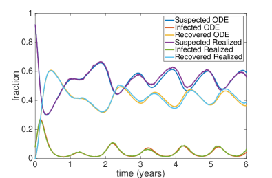
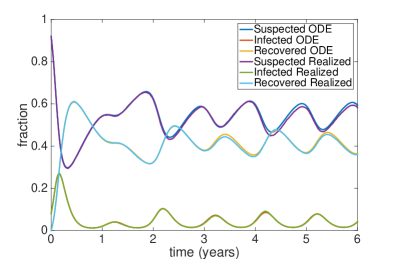
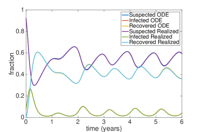
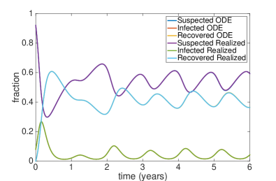
Figure 1: Single realizations of the seasonally forced epidemic model for initial population sizes (a) $N=10^{4}$, (b) $N=10^{5}$, (c) $N=10^{6}$ and (d) $N=10^{7}$, together with the solution of the corresponding deterministic model. Each curve shows the susceptible/ infectious/ recovered fraction (i.e. $S(t)/(S(t)+I(t)+R(t))$, $I(t)/(S(t)+I(t)+R(t))$, and $R(t)/(S(t)+I(t)+R(t))$) against time. Parameter values were chosen as follows: $\beta=20{\rm\ year}^{-1}$, $\beta_{1}=0.4$, $\gamma=10{\rm\ year}^{-1}$ and $\nu=1{\rm\ year}^{-1}$. Parameter values were chosen for illustrative purposes rather than to represent a specific disease in a specific population. In each case, the initial conditions of the system were taken to be $S(0)=0.92N$, $I(0)=0.08N$, with $R(0)=0$.

In order to verify the diffusion-like behavior of $W_{N}(t)$, 4000 realizations of the model were generated. Figure 2(a) shows the distribution of the values of the $j$th component of $W_{N}(1)$ calculated with an initial population size of $N=10^{6}$. As expected, this marginal distribution is consistent with a normal distribution. Furthermore, the mean and standard deviation of this distribution agree with those predicted by the theory. Figure 2(b) shows the distribution of the number of infectives population at time $t=1$ seen across the same set of realizations.

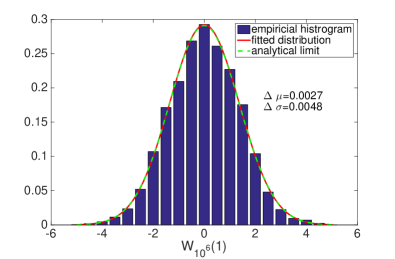
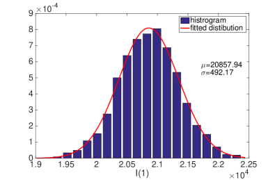
Figure 2: (a) Distribution of the $2$nd component (the component corresponding to the infective) of $W_{10^{6}}(1)$ calculated across 4000 realizations of the model (histogram). The solid red line indicates the best-fitting normal distribution fitted to the empirical histogram. The green dashed curve indicates the normal distribution predicted by the theory. (b) Distribution of the number of infectives seen at time $t=1$ across the same 4000 model realizations. Parameter values and initial conditions were chosen as in Figure 1.

Finally, Figure 3 explores the scaling of the standard deviation of the difference between the realizations and their drift part with the initial population size $N$. For each value of $N$, 4000 realizations of the model were generated and, $\sigma^{i}_{N}(1)$, the standard deviation of the 2nd component of

$$Z_{N}(1)=\xi^{N}_{1}-\xi^{N}_{0}-\int_{0}^{1}F(\xi^{N}_{s},s)ds,$$

was calculated across the set of realizations. We also calculate $f^{i}_{N}(1)$, the mean of fraction of the infectives across the set of realizations. Let

$$R^{i}_{N}(1)=\sigma^{i}_{N}(1)/f^{i}_{N}(1)=O(N^{-1/2})$$

be the ratios between them. The following figure shows, on a log-log scale, this value as a function of $N$. These points fall around a straight line of slope -1/2, consistent with the $1/\sqrt{N}$ scaling predicted by the theory.

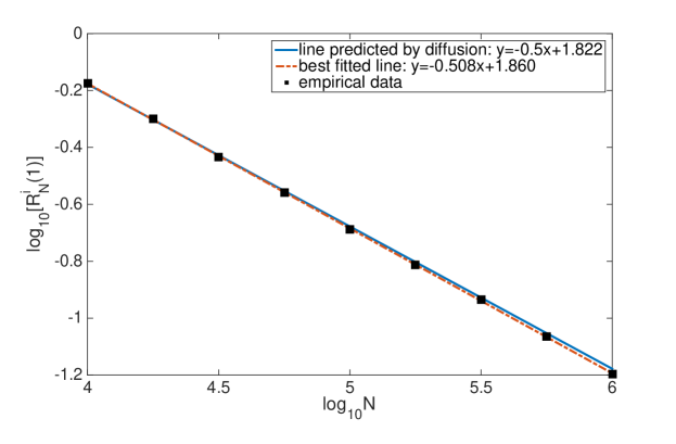
Figure 3: The data points give log-log plot of $R^{i}_{N}(1)$, calculated from 4000 realizations for each $N$ against the population size $N=10^{4},10^{4.25},10^{4.5},\cdots,10^{6}$. The red dashed line gives the best fitted straight using those data points. The blue solid line is the line predicted by Theorem 1 and 2. Parameter values and initial conditions were chosen as in Figure 1.

References

• [1] Anderson, R.M., May, R.M. (1991). Infectious Diseases of Humans. Oxford University Press.
• [2] Bailey, N.T.J. (1950). A simple stochastic epidemic. Biometrika 37: 193-202.
• [3] Bartlett, M.S. (1956). Deterministic and Stochastic Models for Recurrent Epidemics. Pages 81-109. In: Proceedings of the Third Berkeley Symposium on Mathematical Statistics and Probability, vol 4., J. Neyman (ed.), Univ. Calif. Press.
• [4] Bichteler, K. (2002) Stochastic Integration with Jumps, Cambridge University Press, Cambridge
• [5] Durrett, R. (1996). Stochastic Calculus: A Practical Introduction CRC Press, New York.
• [6] Durrett, R. (1995). Ten Lectures on Particle Systems Pages 97–201 in St. Flour Lecture Notes. Lecture Notes in Math 1608. Springer-Verlag, New York.
• [7] Durrett, R., Zhang, Y. (2014). Coexistence of Grass, Saplings and Trees in the Staver-Levin Forest Model arXiv:1401.5220
• [8] Hanson, F. (2007). Applied Stochastic Processes and Control for Jump-Diffusions: Modeling, Analysis and Computation SIAM, Philaelpha.
• [9] Grassly, N.C., Fraser, C. (2006). Seasonal Infectious Disease Epidemiology. Proc. R. Soc. Lond. B 273:2541-2550.
• [10] Lloyd, A. (2004). Estimating Variability in Models for Recurrent Epidemics: Assessing the Use of Moment Closure Techniques Theor. Popul. Biol. 65: 49-65
• [11] Lewis, W., Shedler, S. (1979). Simulation of Nonhomogeneous Poisson Processes by Thinning Naval Research Logistics Quarterly 26 (3): 403
• [12] Isham, V. (1991). Assessing the Variability of Stochastic Epidemics Math Biosci. 107: 209-224
• [13] Kendall, D.G. (1956). Deterministic and Stochastic Epidemics in Closed Populations. Pages 149-165. In: Proceedings of the Third Berkeley Symposium on Mathematical Statistics and Probability, vol 4., J. Neyman (ed.), Univ. Calif. Press.
• [14] Kurtz, T. (1970). Solutions of Ordinary Differential Equations as Limits of Pure Jump Markov Process J. Appl. Prob. 7, 49-58
• [15] Kurtz, T. (1971). Limit Theorem for Sequence of Jump Markov Process J. Appl. Prob. 8, 344-356
• [16] Protter, P. E. (2005). Stochastic Integration and Differential Equations. Springer-Verlag, Berlin.
• [17] Whittle, P. (1957). On the Use of Normal Approximation in the Treatment of Stochastic Processes J. R. Stat. Soc. Ser. B 19: 268-281