Stabilized Quasi-Newton Optimization of Noisy Potential Energy Surfaces

Abstract

Optimizations of atomic positions belong to the most commonly performed tasks in electronic structure calculations. Many simulations like global minimum searches or characterizations of chemical reactions require performing hundreds or thousands of minimizations or saddle computations. To automatize these tasks, optimization algorithms must not only be efficient, but also very reliable. Unfortunately computational noise in forces and energies is inherent to electronic structure codes. This computational noise poses a sever problem to the stability of efficient optimization methods like the limited-memory Broyden–Fletcher–Goldfarb–Shanno algorithm. We here present a technique that allows obtaining significant curvature information of noisy potential energy surfaces. We use this technique to construct both, a stabilized quasi-Newton minimization method and a stabilized quasi-Newton saddle finding approach. We demonstrate with the help of benchmarks that both the minimizer and the saddle finding approach are superior to comparable existing methods.

I Introduction

Stationary points are the most interesting and most important points of potential energy surfaces. The relative energies of local minima and their associated configuration space volumes determine thermodynamic equilibrium properties.David Wales (2003) According to transition state theory, dynamical properties can be deduced from the energies and the connectivity of minima and transition states.Eyring (1935) Therefore, the efficient determination of stationary points of potential energy surfaces is of great interest to the communities of computational chemistry, physics, and biology. Clearly, optimization and in particular minimization problems are present in virtually any field. This explains why the development and mathematical characterization of iterative optimization techniques are important and longstanding research topics, which resulted in a number of highly sophisticated methods like for example direct inversion of the iterative subspace (DIIS),Pulay (1980, 1982) conjugate gradient (CG),Hestenes and Stiefel (1952) or quasi-Newton methods like the Broyden-Fletcher-Goldfarb-Shanno (BFGS) algorithmBroyden (1970); Fletcher (1970); Goldfarb (1970); Shanno (1970) and its limited memory variant (L-BFGS).Nocedal (1980); Liu and Nocedal (1989) Since for a quadratic function Newton’s method is guaranteed to converge within a single iteration, it is not surprising that the BFGS and L-BFGS algorithms belong to the most efficient methods for minimizations of atomic systems.David Wales (2003)

If the potential energy surface can be computed with an accuracy on the order of the machine precision, the above mentioned algorithms usually work extremely well. In practice, however, computing the energy surface at this high precision is not possible for physically accurate but computationally demanding levels of theory like for example density functional theory (DFT). At DFT level, this is due the finitely spaced integration grids and self consistency cycles that have to be stopped at small, but non-vanishing thresholds. Therefore, optimization algorithms that are used at these accurate levels of theory must not only be computationally efficient but also tolerant to noise in forces and energies. Unfortunately, the very efficient L-BFGS algorithm is known to be noise-sensitive and therefore, frequently fails to converge on noisy potential energy surfaces. For this reason, the fast inertial relaxation engine (FIRE) has been developed.Bitzek et al. (2006) FIRE is a method of the damped molecular dynamics (MD) class of optimizers.Tassone, Mauri, and Car (1994); Probert (2003) It accelerates convergence by mixing the velocity at every MD step with a fraction of the current steepest descent direction. A great advantage of FIRE is its simplicity. However, FIRE does not make use of any curvature information and therefore usually is significantly less efficient than the Newton or quasi-Newton methods.

Potential energy surfaces are bounded from below and therefore descent directions guarantee that a local minimum will finally be found. Furthermore, the curvature at a minimum is positive in all directions. This means, all directions can be treated on the same footing during a minimization. The situation is different for saddle point optimizations. A saddle point is a stationary point at which the potential energy surface is at a maximum with respect to one or more particular directions and at a minimum with respect to all other directions. Close to a saddle point it is therefore not possible to treat all directions on the same footing. Instead one has to single out the directions that have to be maximized. Furthermore, far away from a saddle point it is usually impossible to tell, which search direction guarantees to finally end up in a saddle point. Therefore, saddle point optimizations typically are more demanding and significantly less reliable than minimizations.

In this contribution we present a technique that allows to extract curvature information from noisy potential energy surfaces. We explain how to use this technique to construct a stabilized quasi-Newton minimizer (SQNM) and a stabilized quasi-Newton saddle finding method (SQNS). Using benchmarks, we demonstrate that both optimizers are robust and efficient. The comparison of SQNM to L-BFGS and FIRE and of SQNS to an improved dimer methodHenkelman and Jónsson (1999); Kästner and Sherwood (2008) reveals that SQNM and SQNS are superior to their existing alternatives.

II Methods

II.1 Newton’s and Quasi Newton’s Method

The potential energy surface of an $N$-atomic system is a map $E:\mathbb{R}^{3N}\mapsto\mathbb{R}$ that assigns to each atomic configuration $\bm{\mathbf{R}}$ a potential energy. It is assumed that a second order expansion of $E\left(\bm{\mathbf{R}}\right)$ about a point $\bm{\mathbf{R}}^{i}$ is possible:

$$E\left(\bm{\mathbf{R}}\right) \approx E\left(\bm{\mathbf{R}}^{i}\right)+\left[\bm{\mathbf{R}}-\bm{\mathbf{R}}^{i}\right]^{T}\bm{\mathbf{\nabla}}E\left(\bm{\mathbf{R}}^{i}\right)$$

$$\phantom{{}=E\left(\bm{\mathbf{R}}^{i}\right)}+\frac{1}{2}\left[\bm{\mathbf{R}}-\bm{\mathbf{R}}^{i}\right]^{T}H_{\bm{\mathbf{R}}_{i}}\left[\bm{\mathbf{R}}-\bm{\mathbf{R}}^{i}\right]$$ (1)

$$\bm{\mathbf{\nabla}}E\left(\bm{\mathbf{R}}\right) \approx\bm{\mathbf{\nabla}}E\left(\bm{\mathbf{R}}^{i}\right)+H_{\bm{\mathbf{R}}_{i}}\left[\bm{\mathbf{R}}-\bm{\mathbf{R}}^{i}\right],$$ (2)

Here, $H_{\bm{\mathbf{R}}^{i}}$ is the Hessian of the potential energy surface evaluated at $\bm{\mathbf{R}}^{i}$. If $\bm{\mathbf{R}}$ is a stationary point, the left hand side gradient of Eq. 2 vanishes and Newton’s optimization method follows:

$$\bm{\mathbf{R}}^{i+1} =\bm{\mathbf{R}}^{i}-H^{-1}_{\bm{\mathbf{R}}_{i}}\bm{\mathbf{\nabla}}E\left(\bm{\mathbf{R}}^{i}\right)$$ (3)

In the previous equation $\bm{\mathbf{R}}$ was renamed to $\bm{\mathbf{R}}^{i+1}$ in order to emphasize the iterative character of Newton’s Method for non-quadratic potential energy surfaces.

In practice, it is in most cases either impossible to calculate an analytic Hessian or it is too time consuming to compute it numerically by means of finite differences at every iteration. Therefore, quasi-Newton methods use an approximation to the exact Hessian that is computationally less demanding. Using a constant multiple of the identity matrix as an approximation to the Hessian results in the simple steepest descent method. In most cases, such a choice is a very poor approximation to the true Hessian. However, improved approximations can be generated from local curvature information which is obtained from the history of the last $n_{\text{hist}}$ displacements $\bm{\mathbf{\Delta{R}}}^{i}:=\bm{\mathbf{R}}^{i}-\bm{\mathbf{R}}^{i-1}$ and gradient differences $\bm{\mathbf{\Delta{g}}}^{i}:=\bm{\mathbf{\nabla}}E\left(R^{i}\right)-\bm{\mathbf{\nabla}}E\left(\bm{\mathbf{R}}^{i-1}\right)$, where $i=1\dots n_{\text{hist}}$.

II.2 Significant Subspace in Noisy Optimization Problems

In noisy optimization problems, the noisy components of the gradients can lead to displacement components that correspond to erratic movements on the potential energy surface. Consequently, curvature information that comes from the subspace spanned by these displacement components must not be used for the construction of an approximate Hessian. In contrast to this, the non-noisy gradient components promote locally systematic net-movements, which do not tend to cancel each other. In this sense the displacement components that correspond to these well defined net-movement span a significant subspace from which meaningful curvature information can be extracted and used for building an approximate Hessian.

Figure 1: Illustrated are significant subspaces spanned by the displacements in a model atomic coordinate space. Only from the significant subspace it is meaningful to extract curvature information. The red solid arrows simulate displacements made under the influence of noisy forces. The blue dashed arrows show significant subspaces from which it is meaningful to extract curvature information. Panel a) shows a case in which the significant subspace is only one-dimensional. Panel b) shows an example in which curvature information can be extracted from the full 2-dimensional space. The significant subspaces that are shown here were computed using the method outlined in section II.2

The situation is depicted in Fig. 1 where the red solid vectors represent the history of normalized displacements and the blue dashed vectors constitute a basis of the significant subspace. All the red solid vectors in Fig. 1a point into similar directions. Therefore, curvature information should only be extracted from a one-dimensional subspace, as, for example, is given by the blue dashed vector. Displacement components perpendicular to this blue dashed vector come from the noise in the gradients. In contrast to Fig. 1a, Fig. 1b shows a displacement that points into a considerably different direction than all the other displacements. For this reason, significant curvature information can be extracted in the full two-dimensional space.

To define the significant subspace more rigorously, we first introduce the set of normalized displacements

$$\widehat{\bm{\mathbf{\Delta{R}}}}^{i} :=\frac{\bm{\mathbf{\Delta{R}}}^{i}}{|\bm{\mathbf{\Delta{R}}}^{i}|},$$ (4)

where $i=1\dots n_{\text{hist}}$. With $\sum_{k}|\bm{\mathbf{\omega}}_{k}|^{2}=1$, linear combinations $\bm{\mathbf{w}}$ of the normalized displacements are defined as:

$$\bm{\mathbf{w}}:=\sum_{k=1}^{n_{\text{hist}}}\bm{\mathbf{\omega}}_{k}\widehat{\bm{\mathbf{\Delta{R}}}}^{k},$$ (5)

Furthermore, we define a real symmetric overlap matrix $S$ as

$$S_{kl} :=\widehat{\bm{\mathbf{\Delta{R}}}}^{k}\cdot\widehat{\bm{\mathbf{\Delta{R}}}}^{l}.$$ (6)

It can be seen from,

$$\bm{\mathbf{w}}\cdot\bm{\mathbf{w}} =\bm{\mathbf{\omega}}^{T}S\bm{\mathbf{\omega}},$$ (7)

that $|\bm{\mathbf{w}}|$ is made stationary by coefficient vectors $\bm{\mathbf{\omega}}^{i}$ that are eigenvectors of the overlap matrix. In particular the longest and shortest vectors that can be generated by linear combinations with normalized coefficient vectors $\bm{\mathbf{\omega}}$ correspond to those eigenvectors of the overlap matrix that have the largest and smallest eigenvalues. As motivated above, the shortest linear combinations of the normalized displacements correspond to noise.

From now on, let the $\bm{\mathbf{\omega}}^{i}$ be eigenvectors of $\left(S_{kl}\right)$ and let $\lambda_{i}$ be the corresponding eigenvalues. With

$$\stackrel{{\scriptstyle\sim}}{{\smash{\widehat{\bm{\mathbf{\Delta{R}}}}^{i}}\rule{0.0pt}{9.04166pt}}} :=\frac{1}{\sqrt{\lambda_{i}}}\sum_{k=1}^{n_{\text{hist}}}\bm{\mathbf{\omega}}^{i}_{k}\widehat{\bm{\mathbf{\Delta{R}}}}^{k},$$ (8)

we finally define the significant subspace $\mathfrak{S}$ as

$$\mathfrak{S} :=\text{span}\left(\left\{\stackrel{{\scriptstyle\sim}}{{\smash{\widehat{\bm{\mathbf{\Delta{R}}}}^{i}}\rule{0.0pt}{9.04166pt}}}\;\middle|\;\lambda_{i}/\underset{j}{\mathrm{max}}\left\{\lambda_{j}\right\}>\epsilon\right\}\right),$$ (9)

where $0\leq\epsilon\leq 1$. In all applications presented in this work, $\epsilon=10^{-4}$ has proven to work well. Henceforth, we will refer to the dimension of $\mathfrak{S}$ as $n_{\text{dim}}$. By construction it is guaranteed that $n_{\text{dim}}\leq 3N$. It should be noted that at each iteration of the optimization algorithms that are introduced below, the significant subspace and its dimension $n_{\text{dim}}$ can change. The history length $n_{\text{hist}}$ usually lies between 5 and 20.

Our procedure is analogous to Löwdins canonical orthogonalization,Löwdin (1956); Istvan Mayer (2003); Frank Jensen (2007) which is used in the electronic structure community to remove linear dependencies from chemical basis sets.

II.3 Obtaining Curvature Information on the Significant Subspace

We define the projection $\overset{\sim}{H}$ of the Hessian $H$ onto $\mathfrak{S}$ as

$$\overset{\sim}{H} :=PHP$$

$$=\sum_{ij}H_{ij}\stackrel{{\scriptstyle\sim}}{{\smash{\widehat{\bm{\mathbf{\Delta{R}}}}^{i}}\rule{0.0pt}{9.04166pt}}}\left(\stackrel{{\scriptstyle\sim}}{{\smash{\widehat{\bm{\mathbf{\Delta{R}}}}^{j}}\rule{0.0pt}{9.04166pt}}}\right)^{T},$$ (10)

where for all $\stackrel{{\scriptstyle\sim}}{{\smash{\widehat{\bm{\mathbf{\Delta{R}}}}^{i}}\rule{0.0pt}{9.04166pt}}}\in\mathfrak{S}$

$$P:=\sum_{i=1}^{n_{\text{dim}}}\stackrel{{\scriptstyle\sim}}{{\smash{\widehat{\bm{\mathbf{\Delta{R}}}}^{i}}\rule{0.0pt}{9.04166pt}}}\left(\stackrel{{\scriptstyle\sim}}{{\smash{\widehat{\bm{\mathbf{\Delta{R}}}}^{i}}\rule{0.0pt}{9.04166pt}}}\right)^{T}$$

and

$$H_{ij}:=\left(\stackrel{{\scriptstyle\sim}}{{\smash{\widehat{\bm{\mathbf{\Delta{R}}}}^{i}}\rule{0.0pt}{9.04166pt}}}\right)^{T}H\stackrel{{\scriptstyle\sim}}{{\smash{\widehat{\bm{\mathbf{\Delta{R}}}}^{j}}\rule{0.0pt}{9.04166pt}}}.$$

Using Eq. 2 and defining

$$\stackrel{{\scriptstyle\sim}}{{\smash{\bm{\mathbf{\Delta{g}}}^{i}}\rule{0.0pt}{5.59721pt}}} :=\frac{1}{\sqrt{\lambda_{i}}}\sum_{k=1}^{n_{\text{hist}}}\frac{\bm{\mathbf{\omega}}^{i}_{k}}{|\Delta\bm{\mathbf{R}}^{k}|}\Delta\bm{\mathbf{g}}^{k},$$ (11)

where $i=1\dots n_{\text{dim}}$, one obtains an approximation for each matrix element $H_{ij}$:

$${H}_{ij} \approx\stackrel{{\scriptstyle\sim}}{{\smash{\bm{\mathbf{\Delta{g}}}^{i}}\rule{0.0pt}{5.59721pt}}}\cdot\stackrel{{\scriptstyle\sim}}{{\smash{\widehat{\bm{\mathbf{\Delta{R}}}}^{j}}\rule{0.0pt}{9.04166pt}}}.$$ (12)

In practice, we explicitly symmetrize $H_{ij}$ in order to avoid asymmetries introduced by anharmonic effects:

$$H_{ij} \approx\frac{1}{2}\left(\stackrel{{\scriptstyle\sim}}{{\smash{\bm{\mathbf{\Delta{g}}}^{i}}\rule{0.0pt}{5.59721pt}}}\cdot\stackrel{{\scriptstyle\sim}}{{\smash{\widehat{\bm{\mathbf{\Delta{R}}}}^{j}}\rule{0.0pt}{9.04166pt}}}+\stackrel{{\scriptstyle\sim}}{{\smash{\bm{\mathbf{\Delta{g}}}^{j}}\rule{0.0pt}{5.59721pt}}}\cdot\stackrel{{\scriptstyle\sim}}{{\smash{\widehat{\bm{\mathbf{\Delta{R}}}}^{i}}\rule{0.0pt}{9.04166pt}}}\right).$$ (13)

Because the projection $P$ is the identity operator on $\mathfrak{S}$, the curvature $c(\widehat{\bm{\mathbf{d}}})$ on the potential energy surface along a normalized $\widehat{\bm{\mathbf{d}}}\in\mathfrak{S}$ is given by

$$c(\widehat{\bm{\mathbf{d}}}) =\widehat{\bm{\mathbf{d}}}^{T}\overset{\sim}{H}\widehat{\bm{\mathbf{d}}}.$$ (14)

Given the normalized eigenvectors $\bm{\mathbf{v}}^{i}$ and corresponding eigenvalues $\kappa_{i}$ of the $n_{\text{dim}}\times n_{\text{dim}}$ Matrix $\left(H_{ij}\right)$, one can write normalized eigenvectors $\overset{\sim}{\bm{\mathbf{v}}}_{i}\in\mathfrak{S}$ of $\overset{\sim}{H}$ with eigenvalues $\kappa_{i}$ as

$$\overset{\sim}{\bm{\mathbf{v}}}^{i}=\sum_{k=1}^{n_{\text{dim}}}\bm{\mathbf{v}}^{i}_{k}\stackrel{{\scriptstyle\sim}}{{\smash{\widehat{\bm{\mathbf{\Delta{R}}}}^{k}}\rule{0.0pt}{9.04166pt}}},$$ (15)

where $\bm{\mathbf{v}}^{i}_{k}$ is the k-th element of $\bm{\mathbf{v}}^{i}$. As can be seen from Eq. 14, the $\kappa_{i}$ give the curvatures of the potential energy surface along the directions $\overset{\sim}{\bm{\mathbf{v}}}^{i}$.

II.4 Using Curvature Information on the Significant Subspace for Preconditioning $\bm{\mathbf{\nabla}}E$

The gradient $\bm{\mathbf{\nabla}}E$ can be decomposed into a component lying in $\mathfrak{S}$ and a component lying in its orthogonal complement:

$$\bm{\mathbf{\nabla}}E =\bm{\mathbf{\nabla}}E_{\mathfrak{S}}+\bm{\mathbf{\nabla}}E_{\perp},$$ (16)

where $\bm{\mathbf{\nabla}}E_{\mathfrak{S}}:=P^{\prime}\bm{\mathbf{\nabla}}E$, $\bm{\mathbf{\nabla}}E_{\perp}:=(I-P^{\prime})\bm{\mathbf{\nabla}}E$ and $P^{\prime}:=\sum_{i}\overset{\sim}{\bm{\mathbf{v}}}^{i}\left(\overset{\sim}{\bm{\mathbf{v}}}^{i}\right)^{T}$. In this section we motivate how the $\kappa_{i}$ can be used to precondition $\bm{\mathbf{\nabla}}E_{\mathfrak{S}}$. Furthermore, we explain how $\bm{\mathbf{\nabla}}E_{\perp}$ can be scaled appropriately with the help of a feedback that is based on the angle between two consecutive gradients.

Let us assume that the Hessian $H$ at the current point of the potential energy surface is non-singular and let $\nu_{i}$ and $\bm{\mathbf{V}}^{i}$ be its eigenvalues and normalized eigenvectors. In Newton’s Method (Eq. 3), the gradients are conditioned by the inverse Hessian. For the significant subspace component $\bm{\mathbf{\nabla}}E_{\mathfrak{S}}$ it follows:

$$H^{-1}\bm{\mathbf{\nabla}}E_{\mathfrak{S}} =\sum_{i=1}^{3N}\sum_{j=1}^{n_{\text{dim}}}\left[\left(\frac{\bm{\mathbf{\nabla}}E\cdot\overset{\sim}{\bm{\mathbf{v}}}^{j}}{\nu_{i}}\right)\left(\overset{\sim}{\bm{\mathbf{v}}}^{j}\cdot\bm{\mathbf{V}}^{i}\right)\bm{\mathbf{V}}^{i}\right]$$ (17)

As outlined in the previous section, we know the curvature $\kappa_{j}$ along $\overset{\sim}{\bm{\mathbf{v}}}^{j}$. Therefore, at a first thought, Eq. 17 suggests to simply replace $\nu_{i}$ by $\kappa_{j}$ where $i=1\dots 3N$ and $j=1\dots n_{\text{dim}}$. Indeed, if the optimization was restricted to the subspace $\mathfrak{S}$ this choice would be appropriate. However, with respect to the complete domain of the potential energy surface, one is at risk to underestimate the curvature $\nu_{i}$ if the overlap $O_{ij}:=\overset{\sim}{\bm{\mathbf{v}}}^{j}\cdot\bm{\mathbf{V}}^{i}$ is non-vanishing.

In particular, if $O_{ij}$ is far from being negligible, underestimating the curvature $\nu_{i}$ can be particularly problematic because coordinate changes in the direction of $\bm{\mathbf{V}}^{i}$ might be too large. This can render convergence difficult to obtain in practice.

We therefore replace $\nu_{i}$ in Eq. 17 by

$$\kappa_{j}^{\prime}:=\sqrt{\kappa_{j}^{2}+r_{j}^{2}},$$ (18)

where $r_{j}$ is chosen in analogy to the residue of Weinstein’s CriterionWeinstein (1934); Yasuyuki Suzuki and Kalman Varga (1998) as

$$r_{j} :=\left|H\overset{\sim}{\bm{\mathbf{v}}}^{j}-\left((\overset{\sim}{\bm{\mathbf{v}}}^{j})^{T}H\overset{\sim}{\bm{\mathbf{v}}}^{j}\right)\overset{\sim}{\bm{\mathbf{v}}}^{j}\right|.$$ (19)

Using equations 11, 14 and 15, this residue can be approximated by

$$r_{j} \approx\left|\sum_{k=1}^{n_{\text{dim}}}\left[\bm{\mathbf{v}}_{k}^{i}\stackrel{{\scriptstyle\sim}}{{\smash{\bm{\mathbf{\Delta{g}}}^{k}}\rule{0.0pt}{5.59721pt}}}\right]-\kappa_{j}\overset{\sim}{\bm{\mathbf{v}}}^{j}\right|.$$ (20)

With this choice for $\kappa_{j}^{\prime}$, the preconditioned gradient $\bm{\mathbf{\nabla}}E_{\mathfrak{S}}^{\text{P}}$ is finally given by:

$$\bm{\mathbf{\nabla}}E_{\mathfrak{S}}^{\text{P}} :=\sum_{j=1}^{n_{\text{dim}}}\left(\frac{\bm{\mathbf{\nabla}}E\cdot\overset{\sim}{\bm{\mathbf{v}}}^{j}}{\kappa_{j}^{\prime}}\right)\overset{\sim}{\bm{\mathbf{v}}}^{j}.$$ (21)

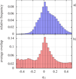
Figure 2: Panel a) is a histogram of $q_{ij}:=\sqrt{\kappa_{j}^{2}+r_{j}^{2}}-\nu_{i}$ for $i=1\dots 3N$ and $j=1\dots n_{\text{dim}}$. $q_{ij}$ is a measure for the quality of the estimation of the eigenvalue $\nu_{i}$ of the exact Hessian. Panel b) shows the bin-averaged overlap $O_{ij}$. The frequency of severe curvature underestimation drops quickly in the region $q_{ij}<0$. The histogram in panel a) peaks in the region of good estimation ($q_{ij}\approx 0$) which coincidences with the region of large overlap $O_{ij}$, shown in panel b). The data for this figure come from 100 minimizations of a $\text{Si}_{20}$ system described by the Lenosky-SiliconLenosky et al. (2000); Goedecker (2002) force field.

Clearly, the residue $r_{j}$ can only alleviate the problem of curvature underestimation, but it does not rigorously guarantee that every single $\nu_{i}$ is estimated appropriately. However, in practice this choice works very well. The reason for this can be seen from Fig. 2. In Fig. 2a, a histogram of the quality and safety measure $q_{ij}:=\sqrt{\kappa_{j}^{2}+r_{j}^{2}}-\nu_{i}$ is shown. If $q_{ij}<0$, the curvature $\nu_{i}$ is underestimated, if $q_{ij}\approx 0$ the curvature $\nu_{i}$ is well estimated and finally, if $q_{ij}>0$, the curvature is overestimated. Overestimation leads to too small step sizes, and therefore to a more stable algorithm, albeit at the cost of a performance loss. Critical underestimation of the curvature ($q_{ij}\ll 0$) is rare. Fig. 2b shows the averages of the overlap $O_{ij}$ in the corresponding bins. If $\overset{\sim}{\bm{\mathbf{v}}}^{j}$ has on average a large overlap with $\bm{\mathbf{V}}^{i}$, the curvature along $\bm{\mathbf{V}}^{i}$ is estimated accurately (histogram in Fig. 2a peaks at $q_{ij}\approx 0$).

What remains to discuss is how the gradient component $\bm{\mathbf{\nabla}}E_{\perp}$ should be scaled. By construction, $\bm{\mathbf{\nabla}}E_{\perp}$ lies in the subspace for which no curvature information is available. We therefore treat this gradient component by a simple steepest descent approach that adjusts the step size $\alpha\in\mathbb{R}^{+}$ at each iteration. For the minimizer that is outlined in section II.6, the adjustment is based on the angle between the complete gradient $\bm{\mathbf{\nabla}}E$ and the preconditioned gradient $\bm{\mathbf{\nabla}}E^{\text{P}}$. If the cosine of this intermediate angle is larger than $0.2$, $\alpha$ is increased by a factor of $1.1$, otherwise $\alpha$ is decreased by a factor of $0.85$. For the saddle search algorithm the feedback is slightly different and will be explained in section II.7.

In conclusion, the total preconditioned gradient $\bm{\mathbf{\nabla}}E^{\text{P}}$ is given by

$$\bm{\mathbf{\nabla}}E^{\text{P}} :=\bm{\mathbf{\nabla}}E_{\mathfrak{S}}^{\text{P}}+\alpha\bm{\mathbf{\nabla}}E_{\perp}$$ (22)

In the next section, we explain how this preconditioned gradient can be further improved for biomolecules.

The preconditioned subspace gradient $\bm{\mathbf{\nabla}}E_{\mathfrak{S}}^{\text{P}}$ was obtained under the assumption of a quadratic potential energy surface. However, if the gradients at the current iteration are large, this assumption is probably not satisfied. Displacing along $\bm{\mathbf{\nabla}}E_{\mathfrak{S}}^{\text{P}}$ in these cases can reduce the stability of the optimization. Hence, if the $|\bm{\mathbf{\nabla}}E|$ exceeds a certain threshold, it can be useful to set the dimension of $\mathfrak{S}$ to zero for a certain number of iterations. This means that $\bm{\mathbf{\nabla}}E_{\perp}=\bm{\mathbf{\nabla}}E$ and therefore $\bm{\mathbf{\nabla}}E^{\text{P}}=\alpha\bm{\mathbf{\nabla}}E$. In that case, $\alpha$ is also adjusted according to the above described gradient feedback. However, as this fallback to steepest descent is intended as a last final fallback, it should have the ability to deal with arbitrarily large forces. Therefore, we also check that $\alpha\bm{\mathbf{\nabla}}E$ does not displace any atom by more than a user-defined trust radius. However, to our experience, this fallback is not necessary in most cases. Indeed, all the benchmarks presented in section III were performed without this fallback.

II.5 Additional Efficiency for Biomolecules

Many large molecules like biomolecules or polymers are floppy systems in which the largest and smallest curvatures can be very different from each other. Steepest descent optimizers are very inefficient for these ill-conditioned systems, because the high curvature directions force to use step sizes that are far too small for an efficient optimization in the directions of small curvatures. Put more formally, the optimization is inefficient for those systems, because the condition number, which is the fraction of largest and smallest curvature, is large.Goedecker, Lancon, and Deutsch (2001) For biomolecules, the high-curvature directions usually correspond to bond stretchings, that is, movements along inter-atomic displacement vectors of bonded atoms. For the current purpose we regard two atoms to be bonded if their inter-atomic distance is smaller than or equal to $1.2$ times the sum of their covalent radii. For $i=1\dots N$, let $\bm{\mathbf{r}}^{i}\in\mathbb{R}^{3}$ be the coordinate vector of the i-th atom. For a system with $n_{\text{bond}}$ bonds we define for each bond a bond vector $\bm{\mathbf{b}}^{m}\in\mathbb{R}^{3N}$, $m=1\dots n_{\text{bond}}$

$$\bm{\mathbf{b}}^{m} :=\left(\begin{matrix}\overset{\sim}{\bm{\mathbf{b}}}^{m,1}\\ \overset{\sim}{\bm{\mathbf{b}}}^{m,2}\\ \vdots\\ \overset{\sim}{\bm{\mathbf{b}}}^{m,N}\end{matrix}\right),$$ (23)

where the $\overset{\sim}{\bm{\mathbf{b}}}^{m,k}\in\mathbb{R}^{3}$, $k=1\dots N$ are defined as

$$\overset{\sim}{\bm{\mathbf{b}}}^{m,i} :=-\overset{\sim}{\bm{\mathbf{b}}}^{m,j} :=\begin{cases}\bm{\mathbf{r}}^{j}-\bm{\mathbf{r}}^{i},&\text{if atoms i and j are}\\ &\text{bonded by the m-th bond}.\\ \bm{\mathbf{0}},&\text{otherwise}.\end{cases}$$ (24)

The $\bm{\mathbf{b}}^{m}$ are sparse vectors with six non-zero elements.

We separate the total gradient $\bm{\mathbf{\nabla}}E$ into its bond-stretching components $\bm{\mathbf{\nabla}}E_{\text{str}}$ and all the remaining components $\bm{\mathbf{\nabla}}E_{\text{r}}$:

$$\bm{\mathbf{\nabla}}E =\bm{\mathbf{\nabla}}E_{\text{str}}+\bm{\mathbf{\nabla}}E_{\text{r}}.$$ (25)

Let $c_{m}\in\mathbb{R}$ be coefficients that allow the bond-stretching components to be expanded in terms of the bond vectors

$$\bm{\mathbf{\nabla}}E_{\text{str}} :=\sum_{m=1}^{n_{\text{bond}}}c_{m}\bm{\mathbf{b}}^{m}.$$ (26)

Using definition Eq. 26, left-multiplying Eq. 25 with a bond vector $\bm{\mathbf{b}}^{n}$ and requiring the $\bm{\mathbf{\nabla}}E_{\text{r}}$ to be orthogonal to all the bond vectors, one obtains the following linear system of equations, which determines the coefficients $c_{m}$ and, with it, the bond stretching gradient defined in Eq. 26:

$$\bm{\mathbf{b}}^{n}\cdot\bm{\mathbf{\nabla}}E =\sum_{m}c_{m}\bm{\mathbf{b}}^{n}\cdot\bm{\mathbf{b}}^{m}.$$ (27)

For the optimization of a biomolecule, the bond-stretching components are minimized in a simple steepest descent fashion. The atoms are displaced by $-\alpha_{\text{s}}\bm{\mathbf{\nabla}}E_{\text{str}}$. The bond-stretching step size $\alpha_{\text{s}}$ is a positive constant, which is adjusted in each iteration of the optimization by simply counting the number of projections $\bm{\mathbf{b}}^{m}\cdot\bm{\mathbf{\nabla}}E$ that have not changed signs since the last iteration. If more than two thirds of the signs of the projections have remained unchanged, the bond-stretching step size $\alpha_{\text{s}}$ is increased by 10 percent. Otherwise, $\alpha_{\text{s}}$ is decreased by a factor of $1/1.1$. The non-bond-stretching gradients $\bm{\mathbf{\nabla}}E_{\text{r}}$ are preconditioned using the stabilized quasi-Newton approach presented in sections II.2 to II.4. It is important to note that in sections II.2 to II.4 all $\bm{\mathbf{\nabla}}E$ have to be replaced by $\bm{\mathbf{\nabla}}E_{\text{r}}$ when using this biomolecule preconditioner. In particular, this is also true for the gradient feedbacks that are described in sections II.4 and II.7.

II.6 Finding Minima – The SQNM method

The pseudo code below demonstrates how the above presented techniques can be assembled into an efficient and stabilized quasi-newton minimizer (SQNM). The pseudo code contains 4 parameters explicitly. $\alpha_{\text{start}}$ and $\alpha_{\text{s,start}}$ are initial step sizes that scale $\bm{\mathbf{\nabla}}E_{\perp}$ and $\bm{\mathbf{\nabla}}E_{\text{str}}$, respectively. $m$ is the maximum length of the history list from which the significant subspace $\mathfrak{S}$ is constructed. $E_{\text{thresh}}$ is an energy-threshold that is used to determine whether a minimization step is accepted or not. It should be adapted to the noise level of the energies and forces. The history list is discarded if the energy increases, because an increase in energy is an indication for inaccurate curvature information. In this case, the dimension of the significant subspace is considered to be zero. Furthermore, line 17 implicitly contains the parameter $\epsilon$, which is described in section II.2. The optimization is considered to be converged if the norm of the gradient is smaller than a certain threshold value. Of course, other force criteria, like for example using the maximum force component instead of the force norm, are possible.

1. $$\alpha\leftarrow\alpha_{\text{start}};\text{ }\alpha_{s}\leftarrow\alpha_{\text{s,start}};$$

2. $$\text{accepted}\leftarrow\text{ true};$$

3. $$k\leftarrow 1;$$

4. $$\text{Initialize }\bm{\mathbf{R}}_{k}\text{ with coordinates;}$$

5. $$E_{k}\leftarrow E(\bm{\mathbf{R}}_{k});$$

6. repeat

7. if optimizing biomolecule then

8. if accepted then

9. Compute $$\bm{\mathbf{\nabla}}E_{\text{str}} \bm{\mathbf{R}}_{k}$$ for , as outlined in section II.5;

10. Adjust $$\alpha_{s}$$ based on the feedback described in section II.5;

11. $$\hskip 64.01866pt\bm{\mathbf{g}}_{k}\leftarrow\bm{\mathbf{\nabla}}E(\bm{\mathbf{R}}_{k})-\bm{\mathbf{\nabla}}E_{\text{str}};$$

12. $$\hskip 64.01866pt\bm{\mathbf{R}}_{k}\leftarrow\bm{\mathbf{R}}_{k}-\alpha_{s}\bm{\mathbf{\nabla}}E_{\text{str}};$$

13. end if

14. else

15. $$\hskip 42.67911pt\bm{\mathbf{g}}_{k}\leftarrow\bm{\mathbf{\nabla}}E(\bm{\mathbf{R}}_{k});$$

16. end if

17. Based on the $$\{\bm{\mathbf{g}}_{j},\bm{\mathbf{R}}_{j}\}_{j\leq k} \bm{\mathbf{\nabla}}E^{\text{P}}$$ in the history list, compute the preconditioned gradient as outlined in sections II.2 to II.5;

18. $$\hskip 21.33955pt\bm{\mathbf{R}}_{k+1}\leftarrow\bm{\mathbf{R}}_{k}-\bm{\mathbf{\nabla}}E^{\text{P}};$$

19. if $$E(\bm{\mathbf{R}}_{k+1})>E_{k}+E_{\text{thresh}} \alpha>\alpha_{\text{start}}/10$$ and then

20. accepted $$\leftarrow$$ false;

21. Remove $$\{\bm{\mathbf{g}}_{j},\bm{\mathbf{R}}_{j}\}_{j<k}$$ from the history list;

22. $$\alpha\leftarrow\alpha/2$$;

23. else

24. accepted $$\leftarrow$$ true;

25. $$E_{k+1}\leftarrow E(\bm{\mathbf{R}}_{k+1})$$;

26. Adjust $$\alpha$$ based on the gradient feedback described in section II.4;

27. $$\hskip 42.67911pt\text{\large{{if }}}k>m\text{\large{{ then}}}$$

28. Remove $$\bm{\mathbf{R}}_{k-m} \bm{\mathbf{g}}_{k-m}$$ and from storage;

29. end if

30. $$\hskip 42.67911ptk\leftarrow k+1;$$

31. end if

32. until convergence.

II.7 Finding Saddle Points – The SQNS Method

In this section we describe a stabilized quasi-Newton saddle finding method (SQNS) that is based on the same principles as the minimizer in the previous section. SQNS belongs to the class of the minimum mode following methods.Cerjan (1981); Wales (1993); Henkelman and Jónsson (1999)

For simplicity, we will denote the Hessian eigenvector corresponding to the smallest eigenvalue as minimum mode. Broadly speaking, a minimum mode following method maximizes along the direction of the minimum mode and it minimzes in all other directions. The optimization is considered to be converged if the curvature along the minimum mode is negative and if the norm of the gradient is smaller than a certain threshold. As for the minimization, other force criteria are possible.

The minimum mode of the Hessian can be found by minimizing the curvature function $c:\mathbb{R}^{3N}\mapsto\mathbb{R}$

$$c(\bm{\mathbf{d}}) =\frac{\bm{\mathbf{d}}^{T}H\bm{\mathbf{d}}}{\bm{\mathbf{d}}^{T}\bm{\mathbf{d}}}$$

$$\approx\frac{\Delta\bm{\mathbf{g}}\cdot\Delta\bm{\mathbf{R}}}{h^{2}},$$ (28)

where along with $h\ll 1$ the following definitions were used: $\Delta\bm{\mathbf{R}}:=h\frac{\bm{\mathbf{d}}}{|\bm{\mathbf{d}}|}$ and $\Delta\bm{\mathbf{g}}:=\bm{\mathbf{\nabla}}E(\bm{\mathbf{R}}+\Delta\bm{\mathbf{R}})-\bm{\mathbf{\nabla}}E(\bm{\mathbf{R}})$. The vector $\bm{\mathbf{R}}$ is the position at which the Hessian $H$ is evaluated at. For the minimization of $c(\bm{\mathbf{d}})$, we use the algorithm described in section II.6 where the energy as objective function is replaced by $c(\bm{\mathbf{d}})$. In the pseudocode below, the here discussed minimization is done at line 6. Under the constraint of normalization, the gradient $\left.\bm{\mathbf{\nabla}}c(\bm{\mathbf{d}})\right|_{|\bm{\mathbf{d}}|=1}$ is given by

$$\left.\bm{\mathbf{\nabla}}c(\bm{\mathbf{d}})\right|_{|\bm{\mathbf{d}}|=1} =2\left(H\bm{\mathbf{d}}-c(\bm{\mathbf{d}})\bm{\mathbf{d}}\right)$$

$$\approx 2\left(\frac{\Delta\bm{\mathbf{g}}}{h}-\left(\frac{\Delta\bm{\mathbf{g}}\cdot\Delta\bm{\mathbf{R}}}{h^{3}}\right)\Delta\bm{\mathbf{R}}\right).$$ (29)

Blindly using the biomolecule preconditioner of section II.5 for the minimization of $c(\bm{\mathbf{d}})$ would mean that the gradient of Eq. 29 was projected on the bond vectors of $\bm{\mathbf{d}}$. Obviously, the bond vector as defined in section II.5 has no meaning for $\bm{\mathbf{d}}$. Therefore, Eq. 29 instead is projected onto the bond vectors of $\bm{\mathbf{R}}+\Delta\bm{\mathbf{R}}$.

At a stationary point, systems with free boundary conditions have six vanishing eigenvalues. The respective eigenvectors correspond to overall translations and rotations.David Wales (2003) Instead of directly using Eq. 29 for the minimization of the curvature of those systems, it is advantageous to remove the translations and rotations from $\Delta\bm{\mathbf{R}}$ and $\left.\bm{\mathbf{\nabla}}c(\bm{\mathbf{d}})\right|_{|\bm{\mathbf{d}}|=1}$ in Eq. 29.Page and McIver (1988); Mills and Jacobsen (1998); David Wales (2003)

The convergence criterion for the minimization of $c(\bm{\mathbf{d}})$ has a large influence on the total number of energy and force evaluations needed to obtain convergence. It therefore must be chosen carefully.

The minimum mode is usually not computed at every iteration, but only if one of the following conditions is fulfilled:

1. at the first iteration of the optimization

2. if the integrated length of the optimization path connecting the current point in coordinate space and the point at which the minimum mode has been calculated the last time exceeds a given threshold value $r_{\text{recomp}}$

3. if the curvature along the minimum mode is positive and the curvature has not been recomputed for at least $n_{\text{recomp}}$ iterations

4. if the curvature along the minimum mode is positive and the norm of the gradient falls below the convergence criterion

5. at convergence (optional)

In the pseudocode, these conditions are checked in line 5. Among these conditions, condition no. 2 is, with respect to the performance, the most important one. The number of energy and gradient evaluations needed for converging to a saddle point can be strongly reduced if a good value for $r_{\text{recomp}}$ is chosen. Condition 3 and 4 can be omitted for most cases. However, for some cases they can offer a slight reduction in the number of energy and gradient evaluations. For example for the alanine dipeptide system used in section III, these two conditions offered a performance gain of almost 10%. Although possible, we usually do not tune $n_{\text{recomp}}$, but typically use $n_{\text{recomp}}=10$. In our implementation, condition 5 is optional. It can be used if very accurate directions of the minimum mode at the saddle point are needed. In this case, this last minimum mode computation can also be done at a tighter convergence criterion. Further energy and gradient computations are saved in our implementation by using the previously computed minimum mode as the starting mode for a new curvature minimization.

As stated above, a saddle point is found by maximizing along the minimum mode and minimizing in all other directions. This is done by inverting the preconditioned gradient component that is parallel to the minimum mode. This is shown at line 19 of the pseudocode below. For the case of biomolecules, the component of the bond-stretching gradient that is parallel to the minimum mode is also inverted (line 13). As already mentioned in section II.4, the feedback that adjusts the stepsize of $\bm{\mathbf{\nabla}}E_{\perp}$ is slightly different in case of the saddle finding method. Let $\widehat{\bm{\mathbf{d}}}_{\text{min}}$ be the normalized direction of the minimum mode. Then, in contrast to minimizations, the stepsize that is used to scale $\bm{\mathbf{\nabla}}E_{\perp}$ is not based on the angle between the complete $\bm{\mathbf{\nabla}}E$ and $\bm{\mathbf{\nabla}}E^{\text{P}}$, but only on the angle between $\bm{\mathbf{\nabla}}E-\left(\bm{\mathbf{\nabla}}E\cdot\widehat{\bm{\mathbf{d}}}_{\text{min}}\right)\widehat{\bm{\mathbf{d}}}_{\text{min}}$ and $\bm{\mathbf{\nabla}}E^{\text{P}}-\left(\bm{\mathbf{\nabla}}E^{\text{P}}\cdot\widehat{\bm{\mathbf{d}}}_{\text{min}}\right)\widehat{\bm{\mathbf{d}}}_{\text{min}}$. These are the components that are responsible for the minimization in directions that are not the minimum mode direction. Otherwise, the gradient feedback is absolutely identical to that described in section II.4.

A saddle point can be higher in energy than the configuration at which the optimization is started at. Therefore, in contrast to a minimization, it is not reasonable to discard the history, if the energy increases. As a replacement for this safeguard, we restore to a simple trust radius approach in which any atom must not be moved by more than a predefined trust radius $r_{\text{trust}}$. A displacement exceeding this trust radius is simply rescaled. If the curvature is positive and the norm of the gradient is below the convergence criterion, we also rescale displacements that do not come from bond-stretchings. The displacement is rescaled such that the displacement of the atom that moved furthest, is finally given by $r_{\text{trust}}$. This avoids arbitrarily small steps close to minima.

On very rare occasions, we could observe for some cluster systems that over the course of several iterations a few atoms sometimes detach from the main cluster. To avoid this problem, we identify the main fragment and move all neighboring fragments towards the nearest atom of the main fragment.

Below, the pseudocode for SQNS is given. It contains 3 parameters explicitly. $\alpha^{\prime}_{\text{start}}$ and $\alpha^{\prime}_{\text{s,start}}$ are initial step sizes that scale $\bm{\mathbf{\nabla}}E_{\perp}$ and $\bm{\mathbf{\nabla}}E_{\text{str}}$, respectively. $m^{\prime}$ is the maximum length of the history list from which the significant subspace is constructed.

The path-length threshold $r_{\text{thresh}}$ that determines the recomputation frequency of the minimum mode is implicitly contained in line 5. Lines 14 and 21 imply the trust radius $r_{\text{trust}}$.

Besides all the parameters that are needed for the minimizer of section II.6, line 6 additionally implies the finite difference step size $h$ that is used to compute the curvature and its gradient.

Line 18 implicitly contains the parameter $\epsilon$, which is described in section II.2

1. $$\alpha^{\prime}\leftarrow\alpha^{\prime}_{\text{start}};\text{ }\alpha^{\prime}_{s}\leftarrow\alpha^{\prime}_{\text{s,start}};$$

2. $$l\leftarrow 1;$$

3. $$\text{Initialize }\bm{\mathbf{R}}_{l}\text{ with coordinates;}$$

4. repeat

5. if recompute minimum mode then

6. Use algorithm of section II.6 and obtain a normalized minimum $$\widehat{\bm{\mathbf{d}}}_{\text{min}} c(\bm{\mathbf{d}}) \bm{\mathbf{R}}_{l}$$ of at , use the previously computed minimum mode as input;

7. end if

8. if optimizing biomolecule then

9. Compute $$\bm{\mathbf{\nabla}}E_{\text{str}} \bm{\mathbf{R}}_{l}$$ for , as outlined in section II.5;

10. Adjust $$\alpha^{\prime}_{s}$$ based on the feedback described in section II.5;

11. $$\hskip 42.67911pt\bm{\mathbf{s}}\leftarrow\alpha^{\prime}_{s}\bm{\mathbf{\nabla}}E_{\text{str}};$$

12. $$\hskip 42.67911pt\bm{\mathbf{g}}_{l}\leftarrow\bm{\mathbf{\nabla}}E(\bm{\mathbf{R}}_{l})-\bm{\mathbf{\nabla}}E_{\text{str}};$$

13. $$\hskip 42.67911pt\bm{\mathbf{R}}_{l}\leftarrow\bm{\mathbf{R}}_{l}-\bm{\mathbf{s}}+2\left(\bm{\mathbf{s}}\cdot\widehat{\bm{\mathbf{d}}}_{\text{min}}\right)\widehat{\bm{\mathbf{d}}}_{\text{min}};$$

14. Check for trust radius condition as described in section II.7. Rescale, if needed;

15. else

16. $$\hskip 42.67911pt\bm{\mathbf{g}}_{l}\leftarrow\bm{\mathbf{\nabla}}E(\bm{\mathbf{R}}_{l});$$

17. end if

18. Based on the $$\{\bm{\mathbf{g}}_{j},\bm{\mathbf{R}}_{j}\}_{j\leq l} \bm{\mathbf{\nabla}}E^{\text{P}}$$ in the history list, compute the preconditioned gradient as outlined in sections II.2 to II.5;

19. $$\hskip 21.33955pt\bm{\mathbf{R}}_{l+1}\leftarrow\bm{\mathbf{R}}_{l}-\bm{\mathbf{\nabla}}E^{\text{P}}+2\left(\bm{\mathbf{\nabla}}E^{\text{P}}\cdot\widehat{\bm{\mathbf{d}}}_{\text{min}}\right)\widehat{\bm{\mathbf{d}}}_{\text{min}};$$

20. Check for trust radius condition and for fragmentation as described in section II.7. Rescale and fix fragmentation, if needed;

21. Adjust $$\alpha^{\prime}$$ based on the gradient feedback described in section II.7;

22. $$\hskip 21.33955pt\text{\large{{if }}}l>m^{\prime}\text{\large{{ then}}}$$

23. Remove $$\bm{\mathbf{R}}_{l-m^{\prime}} \bm{\mathbf{g}}_{l-m^{\prime}}$$ and from the history list;

24. end if

25. $$\hskip 21.33955ptl\leftarrow l+1;$$

26. until convergence.

III Benchmarks and Comparisons

Table 1: Benchmark results for minimizers. DFT test sets contain 100, force field test sets contain 1000 distinct structures. SQNM runs labeled with ’(Bio)’ indicate the usage of the preconditioner for biomolecules described in section II.5.

				To Same Minimum					To Arbitrary Minimum
System	Level of Theory	Method	$n_{\text{f}}$	$N$	$\left<n_{\text{ef}}\right>$	$\left<r\right>$	$\left<n_{\text{woi}}\right>$		$N$	$\left<n_{\text{ef}}\right>$	$\left<r\right>$	$\left<n_{\text{woi}}\right>$
Alanine Dipeptide	DFT	FIRE	0	93	454	14.01	7602		100	458	14.14	7662
		L-BFGS	2	93	185	23.41	3876		100	188	24.02	3941
		SQNM (Bio)	0	93	198	14.10	3711		100	207	14.29	3858
	Force Field	FIRE	0	954	414	12.21	–		1000	418	12.35	–
		L-BFGS	1	954	156	19.69	–		999	158	20.39	–
		SQNM (Bio)	0	954	188	12.38	–		1000	192	12.57	–
		SQNM	0	954	356	12.27	–		1000	363	12.49	–
$\text{Si}_{20}$	DFT	FIRE	0	46	139	18.83	2458		100	143	19.52	2513
		L-BFGS	30	46	73	27.19	1677		70	74	31.26	1714
		SQNM	0	46	83	16.00	1740		100	86	16.50	1784
	Force Field	FIRE	0	486	147	13.26	–		1000	163	15.32	–
		L-BFGS	0	486	57	25.49	–		1000	65	30.44	–
		SQNM	0	486	72	10.82	–		1000	81	11.93	–

III.1 Minimizers

We compare the performance of the new SQNM method to the FIRE and L-BFGS minimizers. We did not include the CG method in this benchmark, because FIRE has previously been shown to be significantly more efficient than CG.Bitzek et al. (2006) Both FIRE and L-BFGS belong to the best optimizers in their class. With regard to the required number of energy and force evaluation, L-BFGS is one of the best minimizers available for the optimization of atomic systems. With respect to noise tolerance, the same is true for FIRE. Although more efficient than FIRE, L-BFGS tends to fail if there are inconsistent forces and energies due to computational noise.Bitzek et al. (2006) Such inconsistencies are unavoidable in electronic structure calculations like for example DFT.

For $\text{Si}_{20}$ clusters and the alanine dipeptide biomolecule, benchmarks were performed both at DFT and force field level. For L-BFGS we used the reference implementation of NocedalNocedal (1980); Liu and Nocedal (1989) which is available from his website. We are not aware of any references implementation of FIRE. However, FIRE is straightforward to implement and thus we used our own code. For the benchmarks of the minimizers at DFT level, all codes were coupled to the BigDFT electronic structure code.Genovese et al. (2008); Mohr et al. (2014) For the benchmarks at force field level, we used the Assisted Model Building with Energy Refinement (AMBER) force field in the ff99SB variant as implemented in AMBER ToolsCase et al. (2014) and the Lenosky Silicon force field.Lenosky et al. (2000); Goedecker (2002)

For alanine dipeptide and $\text{Si}_{20}$, we generated test sets by running MD simulations at force field level. At force field level each test set contains 1000 structures that were taken from the MD trajectories. Subsets containing 100 of these force field structures were used as benchmark systems at DFT level. For each method, we tuned the parameters at force field level for a subset of 100 configurations. Identical parameters were used both at force field and DFT level. The $\text{Si}_{20}$ system was considered to be converged as soon as the norm of the force fell below $1.0\times 10^{-4}$ Hartree/Bohr. Even if far away from a stationary point, relatively small forces can arise in alanine dipeptide. Therefore, a much tighter convergence criterion of $1.0\times 10^{-5}$ Hartree/Bohr had to be chosen for alanine dipeptide.

Table 1 gives the results of these benchmarks. In addition to the average number of energy and force calls $\left<n_{\text{ef}}\right>$ we also give the average integrated path length of the optimization path $\left<r\right>$. $\left<r\right>$ is computed by summing all the distances between structures for which consecutive energy and force evaluations were performed.

There is no guarantee that minimizations that are started at the same configuration will converge to the identical minimum. Therefore, Table 1 gives averages for both, the subset of runs that all converged to identical minima and averages over all runs, regardless of whether the final minima were identical, or not. Identical configurations were identified by using the recently developed s-overlap fingerprints.Sadeghi et al. (2013)

In all benchmarks, FIRE is clearly inferior to L-BFGS and SQNM. With respect to the average number of energy and force evaluations, the L-BFGS method is slightly more efficient than the new SQNM minimizer. However, $\left<r\right>$ of L-BFGS is $1.6$ to $2.6$ times larger than the corresponding values of the SQNM method. On average, this means that L-BFGS displaces the atoms more violently than SQNM. In DFT calculations, the wavefunction of the previous optimization step can be used as input wave function for the current iteration. Roughly speaking, the less the positions of the atoms have changed, the better this input guess usually is. Therefore, less wavefunction optimizations are needed for convergence. To quantify this, the average number of wavefunction optimization iterations $\left<n_{\text{woi}}\right>$ needed for a minimization of the potential energy surface is given in table 1. As a consequence of the smaller displacements in the SQNM method, the L-BFGS and the SQNM method roughly need the same number of wavefunction optimizations for converging to a minimum of the potential energy surface.

The L-BFGS minimizer proved to be unreliable at DFT level. For example, $30\%$ of all $Si_{20}$ minimizations failed to converge. In contrast to this, all SQNM runs successfully converged to a minimum.

III.2 Saddle Finding Methods

Table 2: Benchmark results for saddle finding methods. DFT test sets contain 100, force field test sets contain 1000 distinct structures. SQNS runs labeled with ’(Bio)’ indicate the usage of the preconditioner for biomolecules described in section II.5.

				To Same Saddlepoint			To Arbitrary Saddlepoint
System	Level of Theory	Method	$n_{\text{f}}$	$N$	$\left<n_{\text{ef}}\right>$		$N$	$\left<n_{\text{ef}}\right>$
Alanine Dipeptide	DFT	SQNS	0	–	–		100	510
	Force Field	DIMER	0	87	1324		1000	3146
		SQNS (Bio)	0	87	309		1000	415
		SQNS	0	87	632		1000	757
$\text{Si}_{20}$	DFT	DIMER	0	8	234		100	444
		SQNS	0	8	140		100	237
	Force Field	DIMER	0	20	264		1000	622
		SQNS	0	20	189		1000	368

The SQNS method was compared to an improved version of the dimer methodHenkelman and Jónsson (1999) as described in Ref. 16 and as implemented in the EON code.Chill et al. (2014) In this improved version, the L-BFGSNocedal (1980); Liu and Nocedal (1989); Kästner and Sherwood (2008) algorithm is used for the rotations and translation of the dimer. Furthermore, the rotational force and the dimer energy are evaluated by means of a first order forward finite difference of the gradients.Heyden, Bell, and Keil (2005); Olsen et al. (2004); Kästner and Sherwood (2008) The same force fields as for the minimization benchmarks were used. For the DFT calculations, SQNS was coupled to the BigDFT code. The EON codes offers an interface to VASP,Kresse and Hafner (1993, 1994); Kresse and Furthmüller (1996); Kresse (1996, 1999) which consequently was used.

The same test sets as for the minimizer benchmarks were used. In particular this means that the starting configurations are not close to a saddle point and therefore these test sets are comparatively difficult for saddle finding methods. Again, parameters were only tuned for a subset of 100 configurations at force field level. With exception to the finite difference step size that is needed to calculate the curvature and its gradient, we used the same parameters at force filed and DFT level. Because of noise, the finite difference step size must be chosen larger at DFT level. The same force norm convergence criteria as for the minimization benchmarks were used. In all SQNS optimizations the minimum mode was recalculated at convergence (condition 5 of section II.7).

The test results are given in table 2. In contrast to the minimization benchmarks, we do not give averages for the number wavefunction optimization iterations, because the two saddle finding methods were coupled to two different electronic structure codes. Therefore, the number of wavefunction optimizations is not comparable.

In particular in case of the $\text{Si}_{20}$ system, both methods converged only seldom to the same saddle points and therefore the statistical significance of the corresponding numbers given in table 2 is limited. However, averages over large sets could be made in the case of convergence to an arbitrary saddle point.

In the cases we considered, the dimer method needed between $1.4$ and $7.6$ times more energy and force evaluations than the new SQNS method. In particular for alanine dipeptide, the SQNS approach was far superior to the dimer method. Due to its inefficiency, it was impossible to obtain a significant number of saddle points for alanine dipeptide at DFT level when using the dimer method. For this reason, only benchmark results for the SQNS method are given for alanine dipeptide at DFT level.

IV Conclusion

Optimizations of atomic structures belong to the most important routine tasks in fields like computational physics, chemistry, or biology. Although the energies and forces given by computationally demanding methods like DFT are physically accurate, they are contaminated by noise. This computational noise comes from underlying integration grids and from self-consistency cycles that are stopped at non-vanishing thresholds. The availability of optimization methods that are not only efficient, but also noise-tolerant is therefore of great importance. In this contribution we have presented a technique to extract significant curvature information from noisy potential energy surfaces. We have used this technique to create a stabilized quasi-Newton minimization (SQNM) and a stabilized quasi-Newton saddle finding (SQNS) algorithm. SQNM and SQNS were demonstrated to be superior to existing efficient and well established methods.

Until now, the SQNM and the SQNS optimizers have been used over a period of several months within our group. During this time they have performed thousands of optimizations without failure at the DFT level. Because of their robustness with respect to computational noise and due to their efficiency, they have replaced the default optimizers that have previously been used in Minima HoppingGoedecker (2004); Goedecker, Hellmann, and Lenosky (2005) and Minima Hopping Guided Path SearchSchaefer et al. (2014) runs.

Implementations of the minimizer and the saddle search method are made available via the BigDFT electronic structure package. The code is distributed under the GNU General Public License and can be downloaded free of charge from the BigDFT website.Big