h FR-PHENO-2014-012
h KA-TP-32-2014
h SFB/CPP-14-95
Two-Loop Contributions of the Order $\mathcal{O}(\alpha_{t}\alpha_{s})$
to the Masses of the Higgs Bosons
in the CP-Violating NMSSM

Abstract

We provide the two-loop corrections to the Higgs boson masses of the CP-violating NMSSM in the Feynman diagrammatic approach with vanishing external momentum at ${\cal O}(\alpha_{t}\alpha_{s})$. The adopted renormalization scheme is a mixture between $\overline{\text{DR}}$ and on-shell conditions. Additionally, the renormalization of the top/stop sector is provided both for the $\overline{\text{DR}}$ and the on-shell scheme. The calculation is performed in the gaugeless limit. We find that the two-loop corrections compared to the one-loop corrections are of the order of 5-10%, depending on the top/stop renormalization scheme. The theoretical error on the Higgs boson masses is reduced due to the inclusion of these higher order corrections.

1 Introduction

The discovery of the Higgs boson by the LHC experiments ATLAS [1] and CMS [2] has been a milestone in our quest for understanding the origin of particle masses. While the investigation of the properties of this scalar particle strongly suggests that it is the Higgs boson of the Standard Model (SM), the present precision of the experimental data still leaves room for interpretations in extensions beyond the SM (BSM). Among these, models based on supersymmetry (SUSY) certainly rank among the most intensely studied SM extensions. Supersymmetry allows to cure some of the flaws of the SM. Thus e.g. the symmetry between bosonic and fermionic degrees of freedom solves the hierarchy problem, the inclusion of $R$-parity leads to a possible dark matter candidate and the possibility of additional sources for CP violation provides one of the three necessary conditions for successful baryogenesis. Up to now, however, no SUSY particles have been discovered, and the LHC has put lower limits of around 1.5 TeV on the gluino mass and the squark masses of the first two generations. On the other hand, from analysis strategies based on monojet-like and charm-tagged event selections it can be concluded that the mass of the lightest stop can still be rather light [3, 4, 5, 6, 7, 8, 9], down to about 240 GeV for arbitrary neutralino masses [5]. The stops provide the dominant contribution to the Higgs mass corrections and play a crucial role in pushing the mass of the SM-like SUSY Higgs boson to the necessary 126 GeV. In the minimal supersymmetric extension (MSSM)[10, 11, 12, 13] this requires large values of the stop masses and/or mixing and thus challenges the naturalness of the model due to fine-tuning. The situation is relaxed in the next-to-minimal SUSY extension (NMSSM) [14, 15, 16, 17, 18, 19, 20, 21, 22, 23, 24, 25, 26, 27, 28, 29]: new contributions to the quartic coupling stemming from the introduction of a complex superfield, which couples with the strength $\lambda$ to the two Higgs doublet superfields present in the MSSM, shift the tree-level mass of the lightest CP-even MSSM-like Higgs boson to a higher value. Therefore smaller loop corrections are required to attain the measured Higgs mass value, and lighter stop masses can generate a Higgs spectrum in accordance with the experimental data (see e.g. [30, 31]).

In addition the NMSSM has many other interesting features. It can incorporate CP violation in the Higgs sector already at tree level. The Higgs spectrum may contain Higgs masses that are lighter than 126 GeV without being in conflict with the experimental data, and allowing e.g. for substantial Higgs-to-Higgs decay widths [32, 33, 34, 35]. Also situations with two degenerate Higgs bosons around 126 GeV are possible [30, 31, 36]. This small list already gives a flavour of the plethora of interesting phenomena that are possible in non-minimal SUSY phenomenology. On the other hand it also shows the necessity of precise predictions for the Higgs mass and self-coupling parameters and for the production and the decay processes, i.e. including higher order calculations. In particular in the Higgs sector there has been a lot of activity in pushing the accuracy in the mass calculations to a level comparable to the one achieved in the MSSM. In the CP-conserving NMSSM the leading one-loop (s)top and (s)bottom contributions have been computed in [37, 38, 39, 40, 41] and the chargino, neutralino as well as scalar one-loop contributions at leading logarithmic accuracy have been provided by [42]. The full one-loop contributions in the $\overline{\text{DR}}$ renormalization scheme have first been given in [43] and subsequently in [44]. The authors of [43] have also provided the order ${\cal O}(\alpha_{t}\alpha_{s}+\alpha_{b}\alpha_{s})$ corrections in the approximation of zero external momentum. Recently, first corrections beyond order ${\cal O}(\alpha_{t}\alpha_{s}+\alpha_{b}\alpha_{s})$ have been given in [45]. We have furthermore calculated the full one-loop corrections in the Feynman diagrammatic approach in a mixed $\overline{\text{DR}}$-on-shell and in a pure on-shell renormalization scheme [46]. In the mixed $\overline{\text{DR}}$-on-shell renormalization scheme also the one-loop corrections to the Higgs self-couplings are available [47]. CP-violating effects in the mass corrections have been considered in Refs. [48, 49, 50, 51, 52], where contributions from the third generation squark sector, from the charged particle loops and from gauge boson contributions have been computed in the effective potential approach at one loop-level. The full one-loop and logarithmically enhanced two-loop effects have been made available in the renormalization group approach [53]. We have complemented these calculations by computing the full one-loop corrections in the Feynman diagrammatic approach [54].

There are several codes available for the evaluation of the NMSSM mass spectrum from a user-defined input at a user-defined scale. Thus NMSSMTools [55, 56, 57] calculates the masses and decay widths in the CP-conserving $\mathbb{Z}^{3}$. It can be interfaced with SOFTSUSY [58, 59], which generates the mass spectrum for a CP-conserving NMSSM including the possibility of $\mathbb{Z}^{3}$ violation. The interface of SARAH [60, 61, 62, 63, 45] with SPheno [64, 65] on the other hand allows for spectrum generations of different SUSY models, including the NMSSM. In the same spirit, SARAH has been interfaced with the recently published package FlexibleSUSY [66, 67]. All these programs include the Higgs mass corrections up to two-loop order, where in particular the two-loop corrections are obtained in the effective potential approach. The program package NMSSMCALC [68, 69] for the calculation of the NMSSM Higgs masses and decay widths, incorporates the one-loop corrections in the full Feynman diagrammatic approach both for the CP-conserving and CP-violating NMSSM.

With the present work we contribute to the effort of achieving higher precision in the computation of the NMSSM Higgs boson masses. We provide the two-loop corrections to the neutral NMSSM Higgs boson masses in the Feynman diagrammatic approach for zero external momentum at the order ${\cal O}(\alpha_{t}\alpha_{s})$ based on a mixed $\overline{\text{DR}}$-on-shell renormalization scheme. In contrast to the available results in the effective potential approach we calculate the two-loop corrections not only for the CP-conserving but also for the CP-violating case. In the former case we find full agreement with the results presented in [43]. Our calculation is performed in the gaugeless limit i.e. we set the electric charge and the $W$ and $Z$ boson masses to zero, $e=0,M_{W}=0,M_{Z}=0$. The vacuum expectation value $v$ and the weak angle $\theta_{W}$ are kept at their SM values. Furthermore we neglect the bottom mass. These two-loop mass corrections have been included in the program package NMSSMCALC.

The outline of our paper is as follows. In section 2 we introduce the Higgs sector of the CP-violating NMSSM, and we discuss in particular the quark and squark sector, necessary for the order ${\cal O}(\alpha_{t}\alpha_{s})$ corrections, together with its renormalization. Section 3 is dedicated to the calculation of the mass corrections. Besides presenting the diagrams contributing to the calculation, the counterterms and the applied renormalization prescription are discussed in detail. We furthermore comment on the tools we have used and the checks that we have performed to validate our results. The numerical analysis is deferred to section 4. We show the impact of the two-loop corrections along with the new features that appear with respect to the MSSM. An estimate of the missing higher order corrections is given by applying two different renormalization schemes in the top (s)quark sector. We summarize in section 5.

2 The CP-violating NMSSM

In order to set up our notation, we summarize here the main features of the complex NMSSM, concentrating on those parts of the Lagrangian, that are relevant for the calculation of the ${\cal O}(\alpha_{t}\alpha_{s})$ corrections to the Higgs boson masses, i.e. the Higgs and the stop sectors. For further details and information on other sectors of the CP-violating NMSSM, see Ref. [54]. We work in the framework of the NMSSM with a scale invariant superpotential and a discrete $\mathbb{Z}^{3}$ symmetry. In terms of two Higgs doublet superfields $\hat{H}_{d}$ and $\hat{H}_{u}$, a Higgs singlet superfield $\hat{S}$, the quark and lepton superfields and their charged conjugates (denoted by the superscript $c$), $\hat{Q},\hat{U}^{c},\hat{D}^{c},\hat{L},\hat{E}^{c}$, the NMSSM superpotential reads

$$W_{NMSSM}=\epsilon_{ij}[y_{e}\hat{H}^{i}_{d}\hat{L}^{j}\hat{E}^{c}+y_{d}\hat{H}_{d}^{i}\hat{Q}^{j}\hat{D}^{c}-y_{u}\hat{H}_{u}^{i}\hat{Q}^{j}\hat{U}^{c}]-\epsilon_{ij}\lambda\hat{S}\hat{H}^{i}_{d}\hat{H}^{j}_{u}+\frac{1}{3}\kappa\hat{S}^{3}\;.$$ (2.1)

The indices of the $SU(2)_{L}$ fundamental representation are denoted by $i,j=1,2$, and $\epsilon_{ij}$ is the totally antisymmetric tensor with $\epsilon_{12}=\epsilon^{12}=1$. Here and in the following the summation over equal indices is implicit. The colour and generation indices have been suppressed. The dimensionless parameters $\lambda$ and $\kappa$ are considered to be complex in general. We throughout neglect generation mixing, so that the Yukawa couplings $y_{e},y_{d},y_{u}$ are diagonal and possible complex phases can be reabsorbed by redefining the quark fields without changing the physical meaning [70].

The soft SUSY breaking Lagrangian of the NMSSM expressed in terms of the scalar component fields $H_{u},H_{d}$ and $S$ reads

$${\cal L}_{\text{soft},\text{ NMSSM}}= -m_{H_{d}}^{2}H_{d}^{\dagger}H_{d}-m_{H_{u}}^{2}H_{u}^{\dagger}H_{u}-m_{\tilde{Q}}^{2}\tilde{Q}^{\dagger}\tilde{Q}-m_{\tilde{L}}^{2}\tilde{L}^{\dagger}\tilde{L}-m_{\tilde{u}_{R}}^{2}\tilde{u}_{R}^{*}\tilde{u}_{R}-m_{\tilde{d}_{R}}^{2}\tilde{d}_{R}^{*}\tilde{d}_{R}$$

$$-m_{\tilde{e}_{R}}^{2}\tilde{e}_{R}^{*}\tilde{e}_{R}-(\epsilon_{ij}[y_{e}A_{e}H_{d}^{i}\tilde{L}^{j}\tilde{e}_{R}^{*}+y_{d}A_{d}H_{d}^{i}\tilde{Q}^{j}\tilde{d}_{R}^{*}-y_{u}A_{u}H_{u}^{i}\tilde{Q}^{j}\tilde{u}_{R}^{*}]+h.c.)$$

$$-\frac{1}{2}(M_{1}\tilde{B}\tilde{B}+M_{2}\tilde{W}_{i}\tilde{W}_{i}+M_{3}\tilde{G}\tilde{G}+h.c.)$$ (2.2)

$$-m_{S}^{2}|S|^{2}+(\epsilon_{ij}\lambda A_{\lambda}SH_{d}^{i}H_{u}^{j}-\frac{1}{3}\kappa A_{\kappa}S^{3}+\text{ h.c.})\;,$$

where exemplary for the first generation $\tilde{Q}=(\tilde{u}_{L},\tilde{d}_{L})^{T}$ and $\tilde{L}=(\tilde{\nu}_{L},\tilde{e}_{L})^{T}$ denote the complex scalar components of the corresponding quark and lepton superfields. Working in the CP-violating NMSSM the soft SUSY breaking trilinear couplings $A_{x}$ ($x=\lambda,\kappa,d,u,e$) and the gaugino mass parameters $M_{k}$ ($k=1,2,3$) of the bino, wino and gluino fields $\tilde{B},\tilde{W}_{i}$ ($i=1,2,3$) and $\tilde{G}$ are taken to be complex. By exploiting the $R$-symmetry either $M_{1}$ or $M_{2}$ can chosen to be real. The soft SUSY breaking mass parameters of the scalar fields, $m_{X}^{2}$ ($X=S,H_{d},H_{u},\tilde{Q},\tilde{u}_{R},\tilde{d}_{R},\tilde{L},\tilde{e}_{R}$) are real. A sum over all three quark and lepton generations is implicit.

2.1 The Higgs Sector at Tree Level

From the superpotential, the soft SUSY breaking terms and the $D$-term contributions the Higgs potential is obtained as,

$$V_{H} = (|\lambda S|^{2}+m_{H_{d}}^{2})H_{d,i}^{*}H_{d,i}+(|\lambda S|^{2}+m_{H_{u}}^{2})H_{u,i}^{*}H_{u,i}+m_{S}^{2}|S|^{2}$$

$$+\frac{1}{8}(g_{2}^{2}+g_{1}^{2})(H_{d,i}^{*}H_{d,i}-H_{u,i}^{*}H_{u,i})^{2}+\frac{1}{2}g_{2}^{2}|H_{d,i}^{*}H_{u,i}|^{2}$$

$$+|-\epsilon^{ij}\lambda H_{d,i}H_{u,j}+\kappa S^{2}|^{2}+\big{[}-\epsilon^{ij}\lambda A_{\lambda}SH_{d,i}H_{u,j}+\frac{1}{3}\kappa A_{\kappa}S^{3}+\text{ h.c.}\big{]}\,,$$

where $g_{1}$ and $g_{2}$ denote the $U(1)_{Y}$ and $SU(2)_{L}$ gauge couplings, respectively. The expansion of the two Higgs doublets and the singlet field about their vacuum expectation values, $v_{d},v_{u}$ and $v_{s}$, introduces two additional phases, $\varphi_{u}$ and $\varphi_{s}$,

$$H_{d}=\begin{pmatrix}\frac{1}{\sqrt{2}}(v_{d}+h_{d}+ia_{d})\\ h_{d}^{-}\end{pmatrix},\quad H_{u}=e^{i\varphi_{u}}\begin{pmatrix}h_{u}^{+}\\ \frac{1}{\sqrt{2}}(v_{u}+h_{u}+ia_{u})\end{pmatrix},\quad S=\frac{e^{i\varphi_{s}}}{\sqrt{2}}(v_{s}+h_{s}+ia_{s}).~{}$$ (2.4)

The phase $\varphi_{u}$ enters the top quark mass. In order to keep the top Yukawa coupling real, we absorb this phase into the left-handed and right-handed top fields by replacing

$$t_{L}\to e^{-i\varphi_{u}/2}\,t_{L}\quad\mbox{and}\quad t_{R}\to e^{i\varphi_{u}/2}\,t_{R}\,.$$ (2.5)

This affects all couplings involving one top quark. Substituting Eq. (2.4) into Eq. (2.1), the Higgs potential can be cast into the form

$$V_{H}= V_{H}^{\mbox{\scriptsize const}}+t_{h_{d}}h_{d}+t_{h_{u}}h_{u}+t_{h_{s}}h_{s}+t_{a_{d}}a_{d}+t_{a_{u}}a_{u}+t_{a_{s}}a_{s}$$ (2.6)

$$+\frac{1}{2}\begin{pmatrix}h_{d},h_{u},h_{s},a_{d},a_{u},a_{s}\end{pmatrix}{\mathcal{M}_{\phi\phi}}\begin{pmatrix}h_{d}\\ h_{u}\\ h_{s}\\ a_{d}\\ a_{u}\\ a_{s}\end{pmatrix}+\begin{pmatrix}h_{d}^{+},h_{u}^{+}\end{pmatrix}{\mathcal{M}_{h^{+}h^{-}}}\begin{pmatrix}h_{d}^{-}\\ h_{u}^{-}\end{pmatrix}+V_{H}^{\phi^{3},\phi^{4}}\,,$$

with the tadpole coefficients $t_{\phi}$ ($\phi=h_{d},h_{u},h_{s},a_{d},a_{u},a_{s}$), the $6\times 6$ mass matrix ${\mathcal{M}}_{\phi\phi}$ for the neutral Higgs bosons and the $2\times 2$ mass matrix ${\mathcal{M}}_{h^{+}h^{-}}$ for the charged Higgs bosons. The constant terms are summarized in $V_{H}^{\mbox{\scriptsize const}}$ and the trilinear and quartic Higgs interactions in $V_{H}^{\phi^{3},\phi^{4}}$. The explicit expressions for the tadpoles and mass matrices $\mathcal{M}_{\phi\phi}$ and $\mathcal{M}_{h^{+}h^{-}}$ are given in Ref. [54]. As they are rather lengthy we do not repeat them here, but summarize their main features:

• At tree level, the tadpole coefficients vanish due to the requirement of the Higgs potential taking its minimum at the VEVs $v_{d},v_{u}$ and $v_{s}$. However, only five of the six minimum conditions are actually linearly independent.

• The three phase combinations that appear in the tadpoles and the mass matrices at tree level are given by

  $$\varphi_{x} = \varphi_{A_{\lambda}}+\varphi_{\lambda}+\varphi_{s}+\varphi_{u}\,,$$ (2.7)

  $$\varphi_{y} = \varphi_{\kappa}-\varphi_{\lambda}+2\varphi_{s}-\varphi_{u}\,,$$ (2.8)

  $$\varphi_{z} = \varphi_{A_{\kappa}}+\varphi_{\kappa}+3\varphi_{s}\,.$$ (2.9)

  At lowest order, two of them can be eliminated by exploiting the minimization conditions $t_{a_{d}}=0$ and $t_{a_{s}}=0$. We choose $\varphi_{x}$ and $\varphi_{z}$ to be expressed in terms of $\varphi_{y}$, so that all mass matrix elements mixing the CP-even and CP-odd interaction states, ${\mathcal{M}}_{h_{i}a_{j}}$, are proportional to $\sin\varphi_{y}$. This is the only CP-violating phase that occurs at tree level in the Higgs sector.

• The transformation from the interaction states to the mass eigenstates is performed in two steps. First the would-be Goldstone boson field is separated via rotation by the matrix $\mathcal{R}^{G}$, then the matrix $\mathcal{R}$ is used to rotate to the mass eigenstates,

  $$(h_{d},h_{u},h_{s},a,a_{s},G)^{T} = \mathcal{R}^{G}~{}(h_{d},h_{u},h_{s},a_{d},a_{u},a_{s})^{T}\,,$$

  $$(h_{1},h_{2},h_{3},h_{4},h_{5},G)^{T} = \mathcal{R}~{}(h_{d},h_{u},h_{s},a,a_{s},G)^{T}\,,$$ (2.10)

  with the diagonal mass matrix

  $$\text{diag}(m_{h_{1}}^{2},m_{h_{2}}^{2},m_{h_{3}}^{2},m_{h_{4}}^{2},m_{h_{5}}^{2},0) = \mathcal{R}\mathcal{M}_{hh}\mathcal{R}^{T}\,,\quad\mathcal{M}_{hh}=\mathcal{R}^{G}\mathcal{M}_{\phi\phi}(\mathcal{R}^{G})^{T}.$$ (2.11)

  The mass eigenstates $h_{i}$ ($i=1,...,5$) are ordered by ascending mass, with the lightest mass given by $m_{h_{1}}$.

• The tree-level mass of the charged Higgs boson reads

  $$M_{H^{\pm}}^{2}=M_{W}^{2}+\frac{|\lambda|v_{s}}{s_{2\beta}}\begin{pmatrix}\sqrt{2}|A_{\lambda}|c_{\varphi_{x}}+|\kappa|v_{s}c_{\varphi_{y}}\end{pmatrix}-\frac{|\lambda|^{2}v^{2}}{2}\,,$$ (2.12)

  where here and in the following we use the short hand notations $c_{x}=\cos x,s_{x}=\sin x$ and $t_{x}=\tan x$. The vacuum expectation value $v\approx 246$ GeV is related to $v_{u}$ and $v_{d}$ through $v^{2}=v_{d}^{2}+v_{u}^{2}$.

• The MSSM limit is obtained by $\lambda,\kappa\to 0$ and keeping the parameter $|\mu_{\text{eff}}|=|\lambda|v_{s}/\sqrt{2}$ as well as $A_{\lambda}$ and $A_{\kappa}$ fixed. In this limit the mixing between the singlet and the doublet fields goes to zero.

The set of independent parameters entering the Higgs potential at tree level is chosen to be

$$t_{h_{d}},t_{h_{u}},t_{h_{s}},t_{a_{d}},t_{a_{s}},M_{H^{\pm}}^{2},v,s_{\theta_{W}},e,\tan\beta,|\lambda|,v_{s},|\kappa|,\text{Re}A_{\kappa},s_{\varphi_{y}}\,.$$ (2.13)

There are several changes with respect to the parameter set chosen in Ref. [54]. Here we use $v$ and $s_{\theta_{W}}$ instead of $M_{W}$ and $M_{Z}$, since this is more convenient for the computation of the order ${\cal O}(\alpha_{t}\alpha_{s})$ corrections to the Higgs boson masses, in which we work in the gaugeless limit, i.e. $e=0$ and $M_{W}=M_{Z}=0$ but $v\neq 0$ and $s_{\theta_{W}}\neq 0$. Furthermore the real part of $A_{\kappa}$ is considered rather than the absolute value. In accordance with the SUSY Les Houches Accord (SLHA) [71, 72] conventions we regard the real part as an input parameter and use the tadpole conditions to eliminate the imaginary part of $A_{\kappa}$. For $\lambda$ and $\kappa$ this distinction is not necessary, since both the real and imaginary parts are given in the SLHA convention and can be related to the respective absolute values and phases.

2.2 The Quark and Squark Sector

The two-loop diagrams of the order ${\cal O}(\alpha_{t}\alpha_{s})$ contain coloured particles like top quark, stop, gluon and gluino in the self-energies of the neutral Higgs bosons and additionally bottom quark and sbottom in the charged Higgs self-energy. The stop sector of the complex NMSSM differs from the one of the MSSM due to the appearance of the new complex phase $\varphi_{u}$.

In the gaugeless approximation $e\to 0$, the stop mass matrix reads

$$\mathcal{M}_{\tilde{t}}=\begin{pmatrix}m_{\tilde{Q}_{3}}^{2}+m_{t}^{2}&m_{t}\left(A_{t}^{*}e^{-i\varphi_{u}}-\frac{\mu_{\text{eff}}}{\tan\beta}\right)\\[5.69054pt] m_{t}\left(A_{t}e^{i\varphi_{u}}-\frac{\mu_{\text{eff}}^{*}}{\tan\beta}\right)&m_{\tilde{t}_{R}}^{2}+m_{t}^{2}\end{pmatrix}\,,$$ (2.14)

where the effective higgsino mixing parameter

$$\mu_{\text{eff}}=\frac{\lambda v_{s}e^{i\varphi_{s}}}{\sqrt{2}}$$ (2.15)

has been introduced. The matrix is diagonalized by a unitary matrix $\mathcal{U}_{\tilde{t}}$, rotating the interaction states $\tilde{t}_{L}$ and $\tilde{t}_{R}$ to the mass eigenstates $\tilde{t}_{1}$ and $\tilde{t}_{2}$,

$$(\tilde{t}_{1},\tilde{t}_{2})^{T} = \mathcal{U}_{\tilde{t}}~{}(\tilde{t}_{L},\tilde{t}_{R})^{T},$$ (2.16)

$$\text{diag}(m_{\tilde{t}_{1}}^{2},m_{\tilde{t}_{2}}^{2}) = \mathcal{U}_{\tilde{t}}~{}\mathcal{M}_{\tilde{t}}~{}\mathcal{U}_{\tilde{t}}^{\dagger}\,.$$ (2.17)

In the two-loop diagrams of the charged Higgs self-energy we treat the bottom quark as massless, i.e. $m_{b}=0$. Consequently the left- and right-handed sbottom states do not mix and only the left-handed sbottom with a mass of $m_{\tilde{Q}_{3}}$ contributes. Summarizing, the set of independent parameters entering the top/stop and bottom/sbottom sector is chosen to be

$$m_{t},\;m_{\tilde{Q}_{3}},\;m_{\tilde{t}_{R}}\quad\mbox{and}\quad A_{t}\;.$$ (2.18)

With this parameter choice for the mass matrix in the interaction basis the rotation matrix $\mathcal{U}_{\tilde{t}}$ does not need to be renormalized. This is the same approach as used in the Higgs sector, where we do not renormalize the rotation matrices either.

The parameters in Eq. (2.18) are renormalized at ${\cal O}(\alpha_{s})$. The renormalization can be performed in the on-shell (OS) [73, 74] or $\overline{\text{DR}}$ scheme. For the values of the input parameters we follow the SLHA in which the top quark mass is taken to be the pole mass whereas the soft SUSY breaking masses and trilinear couplings are understood as $\overline{\mbox{DR}}$ parameters evaluated at the renormalization scale $\mu_{R}=M_{\text{SUSY}}$. The latter will be specified in the numerical analysis in Section 4. For the numerical evaluation of the two-loop corrected Higgs boson masses in NMSSMCALC both renormalization schemes have been implemented, and the user has the choice to switch from the default $\overline{\text{DR}}$ scheme to the OS scheme by setting the corresponding flag in the input file. The translation between the two schemes is performed consistently both in the counterterm part and at the level of the input parameters. The OS and $\overline{\mbox{DR}}$ counterterms for any of the parameters $X\equiv m_{t},m_{\tilde{Q}_{3}},m_{\tilde{t}_{R}}$ and $A_{t}$ can be expanded in terms of the dimensional regularization parameter $D=4-2\epsilon$ as

$$\delta X^{\text{OS}} = \frac{1}{\epsilon}\delta X_{\text{pole}}+\delta X_{\text{fin}}\,,$$ (2.19)

$$\delta X^{\overline{\text{DR}}} = \frac{1}{\epsilon}\delta X_{\text{pole}}\,.$$ (2.20)

This fixes the relation between the counterterms in the two schemes. Our definition of the parameters in the OS scheme deliberately does not take into account any terms that are proportional to $\epsilon$, i.e. $\epsilon\delta X_{\epsilon}$. Of course one could also choose to include such terms, that would then manifest themselves as additional finite contributions, due to the counterterm inserted diagrams multiplying $1/\epsilon$ terms from the one-loop functions with the $\epsilon$ parts of the counterterms. We apply our thus defined OS scheme consistently throughout the whole calculation. Choosing the input according to the SLHA and the $\overline{\mbox{DR}}$ scheme as default renormalization scheme, first the $m_{t}^{\overline{\text{DR}}}$ has to be computed from the corresponding OS parameter $m_{t}^{\text{OS}}$ as described in Appendix A. When switching to the OS scheme the translation of the parameters $m_{\tilde{Q}_{3}}^{2},m_{\tilde{t}_{R}}^{2}$ and $A_{t}$ from the $\overline{\mbox{DR}}$ scheme to the OS scheme is performed by applying

$$A_{t}^{(\text{OS})}=A_{t}^{(\overline{\text{DR}})}-\delta A_{t}^{\text{fin}}\;,$$ (2.21)

$$(m_{\tilde{Q}_{L}}^{2})^{(\text{OS})}=(m_{\tilde{Q}_{L}}^{2})^{(\overline{\text{DR}})}-\delta(m_{\tilde{Q}_{L}}^{2})^{\text{fin}}\;,$$ (2.22)

$$(m_{\tilde{t}_{R}}^{2})^{(\text{OS})}=(m_{\tilde{t}_{R}}^{2})^{(\overline{\text{DR}})}-\delta(m_{\tilde{t}_{R}}^{2})^{\text{fin}}\;.$$ (2.23)

Note that we computed the finite counterterm parts in Eqs. (2.21)-(2.23) with OS input parameters. Hence an iterative procedure is required to obtain the OS parameters. The OS conditions for the complex MSSM (s)quark sector, which is the same in the NMSSM, have been presented in Refs. [73] and [74]. For completeness, we list here the expressions for the counterterms.

• The top mass counterterm reads

  $$\delta m_{t}=\frac{1}{2}\widetilde{\text{Re}\!}\;\Big{(}m_{t}\Sigma_{t}^{VL}(m_{t}^{2})+m_{t}\Sigma_{t}^{VR}(m_{t}^{2})+\Sigma_{t}^{SL}(m_{t}^{2})+\Sigma_{t}^{SR}(m_{t}^{2})\Big{)}\,,$$ (2.24)

  where $\widetilde{\text{Re}\!}$ means that the real part is taken only for the one-loop integral function but not for the parameters. The unrenormalized top self-energy $\Sigma_{t}$ is decomposed as

  $$\Sigma_{t}(p^{2})=\not{p}P_{L}\Sigma^{VL}_{t}(p^{2})+\not{p}P_{R}\Sigma^{VR}_{t}(p^{2})+P_{L}\Sigma^{SL}_{t}(p^{2})+P_{R}\Sigma^{SR}_{t}(p^{2})\,,$$ (2.25)

  with the left- and right-handed projectors $P_{L/R}=(1\mp\gamma_{5})/2$.

• The counterterm of the trilinear top coupling is given by

  $$\delta A_{t}=\frac{e^{-i\varphi_{u}}}{m_{t}} \left[\mathcal{U}_{\tilde{t}_{11}}\mathcal{U}_{\tilde{t}_{12}}^{*}(\delta m_{\tilde{t}_{1}}^{2}-\delta m_{\tilde{t}_{2}}^{2})+\mathcal{U}_{\tilde{t}_{11}}\mathcal{U}_{\tilde{t}_{22}}^{*}(\delta Y)^{*}+\mathcal{U}_{\tilde{t}_{21}}\mathcal{U}_{\tilde{t}_{12}}^{*}\delta Y\right.$$ (2.26)

  $$\left.-\left(A_{t}e^{i\varphi_{u}}-\frac{\mu_{\text{eff}}^{*}}{\tan\beta}\right)\delta m_{t}\right]\,,$$

  where

  $$\delta m_{\tilde{t}_{1}}^{2} = \Sigma_{\tilde{t}_{1}\tilde{t}_{1}}(m_{\tilde{t}_{1}}^{2})\,,$$ (2.27)

  $$\delta m_{\tilde{t}_{2}}^{2} = \Sigma_{\tilde{t}_{2}\tilde{t}_{2}}(m_{\tilde{t}_{2}}^{2})\,,$$ (2.28)

  $$\delta Y \equiv \big{[}\mathcal{U}_{\tilde{t}}\delta\mathcal{M}_{\tilde{t}}\mathcal{U}_{\tilde{t}}^{\dagger}\big{]}_{12}=\big{[}\mathcal{U}_{\tilde{t}}\delta\mathcal{M}_{\tilde{t}}\mathcal{U}_{\tilde{t}}^{\dagger}\big{]}^{*}_{21}=\frac{1}{2}\widetilde{\text{Re}}\!\;\Big{(}\Sigma_{\tilde{t}_{1}^{*}\tilde{t}_{2}^{*}}(m_{\tilde{t}_{1}}^{2})+\Sigma_{\tilde{t}_{1}^{*}\tilde{t}_{2}^{*}}(m_{\tilde{t}_{2}}^{2})\Big{)}\,.$$ (2.29)

  We denote by $\Sigma_{\tilde{t}_{i}\tilde{t}_{j}}$ the unrenormalized self-energy for the $\tilde{t}_{i}\rightarrow\tilde{t}_{j}$ transition.

• The counterterm for the soft SUSY breaking left-handed squark mass parameter reads

  $$\delta m_{\tilde{Q}_{L}}^{2}=|\mathcal{U}_{\tilde{t}_{11}}|^{2}\delta m_{\tilde{t}_{1}}^{2}+|\mathcal{U}_{\tilde{t}_{12}}|^{2}\delta m_{\tilde{t}_{2}}^{2}-\mathcal{U}_{\tilde{t}_{22}}\mathcal{U}_{\tilde{t}_{12}}^{*}\delta Y-\mathcal{U}_{\tilde{t}_{12}}\mathcal{U}_{\tilde{t}_{22}}^{*}(\delta Y)^{*}-2m_{t}\delta m_{t}\,.$$ (2.30)

• Finally, the counterterm for the soft SUSY breaking right-handed stop mass parameter is given by

  $$\delta m_{\tilde{t}_{R}}^{2}=|\mathcal{U}_{\tilde{t}_{21}}|^{2}\delta m_{\tilde{t}_{1}}^{2}+|\mathcal{U}_{\tilde{t}_{22}}|^{2}\delta m_{\tilde{t}_{2}}^{2}-\mathcal{U}_{\tilde{t}_{11}}\mathcal{U}_{\tilde{t}_{21}}^{*}(\delta Y)^{*}-\mathcal{U}_{\tilde{t}_{21}}\mathcal{U}_{\tilde{t}_{11}}^{*}\delta Y-2m_{t}\delta m_{t}\,.$$ (2.31)

To complete this subsection, we present the Lagrangians containing the charged Higgs coupling to a top-bottom pair and the top-stop-gluino coupling as well as the charged $W$ boson coupling to top and bottom quark. These are affected by the absorption of the phase related to $v_{u}$ in the top quark field, cf. Eq. (2.5),

$${\cal L}_{t\bar{b}H^{-}} = y_{t}\cos\beta e^{-i\frac{\varphi_{u}}{2}}\bar{b}P_{R}tH^{-}+\text{ h.c.}\;,$$ (2.32)

$${\cal L}_{t\tilde{t}\tilde{g}} = \sqrt{2}g_{s}\bar{\tilde{g}}^{a}\left(-T^{a}_{jk}\mathcal{U}_{\tilde{t}_{i1}}e^{-i\frac{\varphi_{M_{3}}+\varphi_{u}}{2}}P_{L}+T^{a}_{jk}\mathcal{U}_{\tilde{t}_{i2}}e^{i\frac{\varphi_{M_{3}}+\varphi_{u}}{2}}P_{R}\right)t^{k}\tilde{t}^{j*}_{i}+\text{ h.c.}\;,$$ (2.33)

$${\cal L}_{t\bar{b}W^{-}} = -\frac{g_{2}}{\sqrt{2}}e^{-i\frac{\varphi_{u}}{2}}\bar{b}\gamma^{\mu}P_{L}tW^{-}_{\mu}+\text{ h.c.}\;,$$ (2.34)

where $y_{t}=\sqrt{2}m_{t}/(v\sin\beta)$, $i=1,2$ denotes the sfermion mass eigenstate, $j,k=1,2,3$ the $SU(3)$ color indices, $g_{s}$ the strong coupling and $T^{a}$ ($a=1,...,8$) the generators of $SU(3)$.

3 The NMSSM Higgs Boson Masses at Order ${\cal O}(\alpha_{t}\alpha_{s})$

In the Feynman diagrammatic approach, the two-loop Higgs masses are obtained by determining the poles of the propagators, which is equivalent to the calculation of the zeros of the determinant of the two-point function $\hat{\Gamma}(p^{2})$,

$$\text{Det}\left(\hat{\Gamma}(p^{2})\right)=0\;,\quad\text{with}\quad\left(\hat{\Gamma}(p^{2})\right)_{ij}=i\delta_{ij}\left(p^{2}-m_{h_{i}}^{2}\right)+i\hat{\Sigma}_{ij}(p^{2})\;,\qquad i,j=1...5\;,$$ (3.35)

where $m_{h_{i}}$ are the tree-level masses and $\hat{\Sigma}_{ij}(p^{2})$ is the renormalized self-energy of the $h_{i}\rightarrow h_{j}$ transition at $p^{2}$. Note that $h_{i/j}$ denote the tree-level mass eigenstates. We have neglected the higher order corrections due to the mixing of the Goldstone boson with the remaining neutral Higgs bosons. This mixing has been verified numerically to be negligible. For the evaluation of the loop-corrected Higgs masses and Higgs mixing matrix, we follow the numerical procedure given in Refs.[46, 54].

The renormalized self-energies of the Higgs bosons, $\hat{\Sigma}_{ij}$, contain one-loop and two-loop contributions, which are labeled with the superscript (1) and (2), respectively,

$$\hat{\Sigma}_{ij}(p^{2})=\hat{\Sigma}_{ij}^{(1)}(p^{2})+\hat{\Sigma}_{ij}^{(2)}(0)\;.$$ (3.36)

The one-loop renormalized self-energies have been discussed in detail in Refs. [46] and [54]. Here we concentrate only on the two-loop parts, $\hat{\Sigma}_{ij}^{(2)}(0)$. They are evaluated at vanishing external momentum $p^{2}=0$ and can be decomposed as

$$\hat{\Sigma}^{(2)}_{h_{i}h_{j}}(0)=\Sigma^{(2)}_{h_{i}h_{j}}(0)-\frac{1}{2}\Big{[}\mathcal{R}\Big{(}(\delta^{\text{\tiny(}\!\text{\tiny 2}\!\text{\tiny)}}\!\mathcal{Z})^{\dagger}\mathcal{M}_{hh}+\mathcal{M}_{hh}\delta^{\text{\tiny(}\!\text{\tiny 2}\!\text{\tiny)}}\!\mathcal{Z}\Big{)}\mathcal{R}^{T}\Big{]}_{ij}-\Big{(}\mathcal{R}\delta^{\text{\tiny(}\!\text{\tiny 2}\!\text{\tiny)}}\!\mathcal{M}_{hh}\mathcal{R}^{T}\Big{)}_{ij}\,,$$ (3.37)

where the first term, $\Sigma^{(2)}_{h_{i}h_{j}}$, denotes the unrenormalized self-energy, the second term contains the wave function renormalization constants with

$$\delta^{\text{\tiny(}\!\text{\tiny 2}\!\text{\tiny)}}\!\mathcal{Z}=\text{diag}(\delta^{\text{\tiny(}\!\text{\tiny 2}\!\text{\tiny)}}\!Z_{H_{d}},\delta^{\text{\tiny(}\!\text{\tiny 2}\!\text{\tiny)}}\!Z_{H_{u}},\delta^{\text{\tiny(}\!\text{\tiny 2}\!\text{\tiny)}}\!Z_{S},s_{\beta}^{2}\delta^{\text{\tiny(}\!\text{\tiny 2}\!\text{\tiny)}}\!Z_{H_{d}}+c_{\beta}^{2}\delta^{\text{\tiny(}\!\text{\tiny 2}\!\text{\tiny)}}\!Z_{H_{u}},\delta^{\text{\tiny(}\!\text{\tiny 2}\!\text{\tiny)}}\!Z_{S})\,,$$ (3.38)

and the third term includes the two-loop counterterm mass matrix $\delta^{\text{\tiny(}\!\text{\tiny 2}\!\text{\tiny)}}\!\mathcal{M}_{hh}$. The neutral Higgs mass matrix $\mathcal{M}_{hh}$ and the rotation matrix $\mathcal{R}$ correspond to the ones defined in Eqs. (2.10) and (2.11) after dropping the Goldstone component. The counterterm constants appearing in Eq. (3.37) will be discussed in detail in Subsection 3.2.

3.1 The Unrenormalized Self-Energies of the Neutral Higgs Bosons

Figure 1: Sample diagrams of genuine two-loop corrections contributing to the neutral Higgs boson self-energies at $\mathcal{O}(\alpha_{t}\alpha_{s})$, with tops ($t$), stops ($\tilde{t}_{1},\tilde{t}_{2}$), gluons ($g$) and gluinos ($\tilde{G}$) in the loops and $k,l,m,n=1,2$, $i,j=1,...,5$.

Figure 2: Examples of counterterm inserted diagrams contributing to the neutral Higgs boson self-energies.

The unrenormalized self-energies of the transitions $h_{i}\rightarrow h_{j}$ consist of the contributions from genuine two-loop diagrams and from counterterm inserted one-loop diagrams. The genuine two-loop diagrams must contain either a gluon or gluino or four-stop couplings. Some example diagrams are presented in Fig. 1. After performing the tensor reduction of these diagrams at zero external momentum, an expression in terms of either one two-loop vacuum integral or of products of two one-loop vacuum integrals is obtained. The counterterm inserted one-loop diagrams, which are shown in Fig. 2, contain either coupling-type counterterms or propagator-type counterterms of top quarks and stops. The set of counterterms involved in these diagrams has been discussed in Subsection 2.2. For the evaluation of these counterterms also the one-loop two-point functions with full momentum dependence are needed. The one-loop and the two-loop master integrals have to be expanded in terms of the dimensional regularization parameter $D=4-2\epsilon$. The one-loop one-point and two-point functions have been defined in [75, 76]. For the two-loop vacuum functions we use the existing results in [77, 78, 79, 80, 81, 82, 83]. Inserting these expansions into the two-loop expressions, we can easily extract the coefficients of the double pole, single pole and finite parts. After gaining such expressions also for the counterterms of the relevant parameters we can explicitly check the cancellation of the UV divergences.

3.2 The Counterterms

When calculating the $\mathcal{O}(\alpha_{t}\alpha_{s})$ corrections, we employ the gaugeless limit i.e. $e\to 0$. This leads to the independence of the Higgs potential on $s_{\theta_{W}}$. Therefore we restrict ourselves to a new set of independent parameters entering the Higgs potential at order ${\cal O}(\alpha_{t}\alpha_{s})$,

$$t_{h_{d}},t_{h_{u}},t_{h_{s}},t_{a_{d}},t_{a_{s}},M_{H^{\pm}}^{2},v,\tan\beta,|\lambda|,v_{s},|\kappa|,\text{Re}A_{\kappa},s_{\varphi_{y}}\,.$$ (3.39)

In order to obtain a UV-finite result, these parameters need to be renormalized. The parameters are replaced by the renormalized ones and the corresponding counterterms according to

$$t_{\phi} \rightarrow t_{\phi}+\delta^{\text{\tiny(}\!\text{\tiny 1}\!\text{\tiny)}}\!t_{\phi}+\delta^{\text{\tiny(}\!\text{\tiny 2}\!\text{\tiny)}}\!t_{\phi}\qquad\qquad\quad\text{with}~{}~{}\phi=h_{d},h_{u},h_{s},a_{d},a_{s}\;,$$ (3.40)

$$M_{H^{\pm}}^{2} \rightarrow M_{H^{\pm}}^{2}+\delta^{\text{\tiny(}\!\text{\tiny 1}\!\text{\tiny)}}\!M_{H^{\pm}}^{2}+\delta^{\text{\tiny(}\!\text{\tiny 2}\!\text{\tiny)}}\!M_{H^{\pm}}^{2}\;,$$ (3.41)

$$v \rightarrow v+\delta^{\text{\tiny(}\!\text{\tiny 1}\!\text{\tiny)}}\!v+\delta^{\text{\tiny(}\!\text{\tiny 2}\!\text{\tiny)}}\!v\;,$$ (3.42)

$$\tan\beta \rightarrow\tan\beta+\delta^{\text{\tiny(}\!\text{\tiny 1}\!\text{\tiny)}}\!\tan\beta+\delta^{\text{\tiny(}\!\text{\tiny 2}\!\text{\tiny)}}\!\tan\beta\;,$$ (3.43)

$$v_{s} \rightarrow v_{s}+\delta^{\text{\tiny(}\!\text{\tiny 1}\!\text{\tiny)}}\!v_{s}+\delta^{\text{\tiny(}\!\text{\tiny 2}\!\text{\tiny)}}\!v_{s}\;,$$ (3.44)

$$|\lambda| \rightarrow|\lambda|+\delta^{\text{\tiny(}\!\text{\tiny 1}\!\text{\tiny)}}\!|\lambda|+\delta^{\text{\tiny(}\!\text{\tiny 2}\!\text{\tiny)}}\!|\lambda|\;,$$ (3.45)

$$|\kappa| \rightarrow|\kappa|+\delta^{\text{\tiny(}\!\text{\tiny 1}\!\text{\tiny)}}\!|\kappa|+\delta^{\text{\tiny(}\!\text{\tiny 2}\!\text{\tiny)}}\!|\kappa|\;,$$ (3.46)

$$\text{Re}A_{\kappa} \rightarrow\text{Re}A_{\kappa}+\delta^{\text{\tiny(}\!\text{\tiny 1}\!\text{\tiny)}}\!\text{Re}A_{\kappa}+\delta^{\text{\tiny(}\!\text{\tiny 2}\!\text{\tiny)}}\!\text{Re}A_{\kappa}\;,$$ (3.47)

$$s_{\varphi_{y}} \rightarrow s_{\varphi_{y}}+\delta^{\text{\tiny(}\!\text{\tiny 1}\!\text{\tiny)}}\!s_{\varphi_{y}}+\delta^{\text{\tiny(}\!\text{\tiny 2}\!\text{\tiny)}}\!s_{\varphi_{y}}\;,$$ (3.48)

where the superscript $(n)$ denotes the $n$-loop level. The one-loop counterterms are of course not of order ${\cal O}(\alpha_{t}\alpha_{s})$ and have been defined explicitly in Ref. [54]. Therefore we restrict ourselves here to the discussion of the two-loop counterterms only. To ensure consistency of our one- and two-loop corrections we apply the same mixed $\overline{\text{DR}}$-on-shell renormalization scheme as in Ref. [54], in particular,

$$\underbrace{t_{h_{d}},t_{h_{u}},t_{h_{s}},t_{a_{d}},t_{a_{s}},M_{H^{\pm}}^{2},v}_{\mbox{on-shell scheme}},\underbrace{\tan\beta,|\lambda|,v_{s},|\kappa|,\text{Re}A_{\kappa},s_{\varphi_{y}}}_{\overline{\mbox{DR}}\mbox{ scheme}}\,.$$ (3.49)

Inserting the replacements given in Eqs. (3.40)-(3.48) in the mass matrix, the counterterm matrix for the neutral Higgs mass matrix $\mathcal{M}_{hh}$ is obtained,

$$\mathcal{M}_{hh}\rightarrow\mathcal{M}_{hh}+\delta^{\text{\tiny(}\!\text{\tiny 1}\!\text{\tiny)}}\!\mathcal{M}_{hh}+\delta^{\text{\tiny(}\!\text{\tiny 2}\!\text{\tiny)}}\!\mathcal{M}_{hh}\;.$$ (3.50)

In Appendix B, we give the explicit expressions of $\delta^{\text{\tiny(}\!\text{\tiny 2}\!\text{\tiny)}}\!\mathcal{M}_{hh}$ in terms of all OS parameter counterterms.

In addition to the set of independent parameters of Eq. (3.49), the Higgs field wave functions need to be renormalized. The renormalization constants for the doublet and singlet fields are introduced before rotating to the mass eigenstates as

$$H_{d} \rightarrow (1+\frac{1}{2}\delta^{\text{\tiny(}\!\text{\tiny 1}\!\text{\tiny)}}\!Z_{H_{d}}+\frac{1}{2}\delta^{\text{\tiny(}\!\text{\tiny 2}\!\text{\tiny)}}\!Z_{H_{d}})H_{d}\;,$$ (3.51)

$$H_{u} \rightarrow (1+\frac{1}{2}\delta^{\text{\tiny(}\!\text{\tiny 1}\!\text{\tiny)}}\!Z_{H_{u}}+\frac{1}{2}\delta^{\text{\tiny(}\!\text{\tiny 2}\!\text{\tiny)}}\!Z_{H_{u}})H_{u}\;,$$ (3.52)

$$S \rightarrow (1+\frac{1}{2}\delta^{\text{\tiny(}\!\text{\tiny 1}\!\text{\tiny)}}\!Z_{S}+\frac{1}{2}\delta^{\text{\tiny(}\!\text{\tiny 2}\!\text{\tiny)}}\!Z_{S})S\;.$$ (3.53)

The counterterms for the renormalized parameters and the field renormalization constants are fixed via the renormalization conditions, listed in the following:

• Analogously to the one-loop calculation the field renormalization constants are given via $\overline{\text{DR}}$ conditions defined as

  $$\delta^{\text{\tiny(}\!\text{\tiny 2}\!\text{\tiny)}}\!Z_{H_{d}}=-\left.\frac{\partial\Sigma^{(2)}_{h_{d}h_{d}}}{\partial p^{2}}\right|_{\text{div}}(p^{2}\to 0)\,,$$ (3.54)

  $$\delta^{\text{\tiny(}\!\text{\tiny 2}\!\text{\tiny)}}\!Z_{H_{u}}=-\left.\frac{\partial\Sigma^{(2)}_{h_{u}h_{u}}}{\partial p^{2}}\right|_{\text{div}}(p^{2}\to 0)\,,$$ (3.55)

  $$\delta^{\text{\tiny(}\!\text{\tiny 2}\!\text{\tiny)}}\!Z_{S}=-\left.\frac{\partial\Sigma^{(2)}_{h_{s}h_{s}}}{\partial p^{2}}\right|_{\text{div}}(p^{2}\to 0)\,,$$ (3.56)

  where the subscript ’div’ denotes the divergent part. It turns out that at order ${\cal O}(\alpha_{t}\alpha_{s})$ $\delta^{\text{\tiny(}\!\text{\tiny 2}\!\text{\tiny)}}\!Z_{H_{d}}$ and $\delta^{\text{\tiny(}\!\text{\tiny 2}\!\text{\tiny)}}\!Z_{S}$ are zero.

  Using $\overline{\text{DR}}$ renormalization in the top/stop sector the non-vanishing field renormalization constant $\delta^{\text{\tiny(}\!\text{\tiny 2}\!\text{\tiny)}}\!Z_{H_{u}}$ is given by

  $$\delta^{\text{\tiny(}\!\text{\tiny 2}\!\text{\tiny)}}\!Z_{H_{u}}^{\overline{\text{DR}}}=\frac{\alpha_{s}(m_{t}^{2})^{\overline{\text{DR}}}}{8\pi^{2}v^{2}\sin^{2}\beta}\left(\frac{1}{\epsilon^{2}}-\frac{1}{\epsilon}\right),$$ (3.57)

  which is in agreement with the result as obtained in the MSSM [84]. If instead one uses on-shell renormalization for the top mass, the counterterm inserted one-loop diagrams will lead to an additional contribution to the field renormalization constant, which is then

  $$\delta^{\text{\tiny(}\!\text{\tiny 2}\!\text{\tiny)}}\!Z_{H_{u}}^{\text{OS}}=\frac{\alpha_{s}(m_{t}^{2})^{\text{OS}}}{8\pi^{2}v^{2}\sin^{2}\beta}\left(\frac{1}{\epsilon^{2}}-\frac{1}{\epsilon}\right)-\frac{3}{4\pi^{2}}\frac{m_{t}^{\text{OS}}(\delta m_{t})_{\text{fin}}}{v^{2}\sin^{2}\beta}\frac{1}{\epsilon}\,,$$ (3.58)

  where $(\delta m_{t})_{\text{fin}}$ is the finite part of the top mass counterterm as defined in Eq. (2.19) and which is given by

  $$(\delta m_{t})_{\text{fin}}= \frac{\alpha_{s}m_{t}}{3\pi}\Big{[}3\log\Big{(}\frac{m_{t}^{2}}{\mu_{R}^{2}}\Big{)}-5\Big{]}+dm_{t}\;.$$ (3.59)

  Here $dm_{t}$ is the SUSY-QCD correction given in Eq. (A.95). However, we would like to point out that the complete wave function renormalization constant is the same up to higher orders and independent of the renormalization scheme used for the top mass. This can easily be seen, when looking at the sum of the one- and two-loop counterterm $\delta Z_{H_{u}}$. At one-loop level, if one takes only the top/stop contribution then $\delta^{\text{\tiny(}\!\text{\tiny 1}\!\text{\tiny)}}\!Z_{H_{d}}$ and $\delta^{\text{\tiny(}\!\text{\tiny 1}\!\text{\tiny)}}\!Z_{S}$ are also zero and

  $$\delta^{\text{\tiny(}\!\text{\tiny 1}\!\text{\tiny)}}\!Z_{H_{u}}=-\frac{3m_{t}^{2}}{8\pi^{2}v^{2}\sin^{2}\beta}\frac{1}{\epsilon}\;.$$ (3.60)

  Hence, the sum of the one- and two-loop contribution is given by

  $$\delta Z_{H_{u}}^{\overline{\text{DR}}} =\underbrace{-\frac{3(m_{t}^{2})^{\overline{\text{DR}}}}{8\pi^{2}v^{2}\sin^{2}\beta}\frac{1}{\epsilon}}_{\text{one-loop}}+\underbrace{\frac{\alpha_{s}(m_{t}^{2})^{\overline{\text{DR}}}}{8\pi^{2}v^{2}\sin^{2}\beta}\left(\frac{1}{\epsilon^{2}}-\frac{1}{\epsilon}\right)}_{\text{two-loop}},$$ (3.61)

  $$\delta Z_{H_{u}}^{\text{OS}} =\underbrace{-\frac{3(m_{t}^{2})^{\text{OS}}}{8\pi^{2}v^{2}\sin^{2}\beta}\frac{1}{\epsilon}}_{\text{one-loop}}+\underbrace{\frac{\alpha_{s}(m_{t}^{2})^{\text{OS}}}{8\pi^{2}v^{2}\sin^{2}\beta}\left(\frac{1}{\epsilon^{2}}-\frac{1}{\epsilon}\right)-\frac{3}{4\pi^{2}}\frac{m_{t}^{\text{OS}}(\delta m_{t})_{\text{fin}}}{v^{2}\sin^{2}\beta}\frac{1}{\epsilon}}_{\text{two-loop}}.$$ (3.62)

  Taking into account the relation $m_{t}^{\overline{\text{DR}}}=m_{t}^{\text{OS}}+(\delta m_{t})_{\text{fin}}$, it is evident that $\delta Z_{H_{u}}^{\overline{\text{DR}}}$ and $\delta Z_{H_{u}}^{\text{OS}}$ agree up to higher orders.

• The renormalization conditions for the tadpoles are chosen such that the minimum of the Higgs potential does not change when it receives two-loop corrections, leading to

  $$\delta^{\text{\tiny(}\!\text{\tiny 2}\!\text{\tiny)}}\!t_{\phi}=t_{\phi}^{(2)}\;,\quad\phi=(h_{d},h_{u},h_{s},a_{d},a_{s})\;.$$ (3.63)

  Sample two-loop tadpole and counterterm inserted tadpole diagrams are shown in Fig. 3.

  

  Figure 3: Sample two-loop tadpole and counterterm inserted tadpole diagrams at $\mathcal{O}(\alpha_{t}\alpha_{s})$ for the neutral Higgs bosons.

• The charged Higgs boson mass is defined as an OS parameter. Hence,

  $$\delta^{\text{\tiny(}\!\text{\tiny 2}\!\text{\tiny)}}\!M_{H^{\pm}}^{2} =\Sigma_{H^{\pm}}^{(2)}(0)-M_{H^{\pm}}^{2}(\cos^{2}\!\beta\delta^{\text{\tiny(}\!\text{\tiny 2}\!\text{\tiny)}}\!Z_{H_{u}}+\sin^{2}\!\beta\delta^{\text{\tiny(}\!\text{\tiny 2}\!\text{\tiny)}}\!Z_{H_{d}})\,.$$ (3.64)

  The two-loop corrections to the mass of the charged Higgs boson are also calculated at vanishing external momentum. Therefore the counterterm for the mass of the charged Higgs boson is not solely fixed by the unrenormalized self-energy, but is also related to the field renormalization constants. Note, however, that this of course does not affect the finite part. Some examples of two-loop diagrams contributing to the unrenormalized self-energy of the charged Higgs boson are shown in Fig. 4 (upper row). In addition to top quarks and squarks, gluons and gluinos also bottom quarks and squarks appear in the loops. We perform our calculation in the limit of vanishing bottom mass and neglect the $D$-term in the sbottom mass matrix. Therefore the left- and right-handed sbottoms do not mix, and only the left-handed sbottom contributes. The counterterm of the soft SUSY breaking left-handed squark mass parameter needed in the calculation of the one-loop inserted counterterm diagrams has been given in Subsection 2.2. Some example diagrams are given in Fig. 4 (lower row).

  

  Figure 4: Sample two-loop and counterterm inserted diagrams at $\mathcal{O}(\alpha_{t}\alpha_{s})$ contributing to the charged Higgs boson self-energy.

  

  Figure 5: Sample two-loop and counterterm inserted diagrams at $\mathcal{O}(\alpha_{t}\alpha_{s})$ contributing to the $W$, respectively $Z$ boson self-energies.

• The counterterm $\delta^{\text{\tiny(}\!\text{\tiny 2}\!\text{\tiny)}}\!v/v$ is taken to be an OS parameter and hence

  $$\frac{\delta^{\text{\tiny(}\!\text{\tiny 2}\!\text{\tiny)}}\!v}{v}=\frac{c_{\theta_{W}}^{2}}{2s_{\theta_{W}}^{2}}\left(\frac{\delta^{\text{\tiny(}\!\text{\tiny 2}\!\text{\tiny)}}\!M_{Z}^{2}}{M_{Z}^{2}}-\frac{\delta^{\text{\tiny(}\!\text{\tiny 2}\!\text{\tiny)}}\!M_{W}^{2}}{M_{W}^{2}}\right)+\frac{\delta^{\text{\tiny(}\!\text{\tiny 2}\!\text{\tiny)}}\!M_{W}^{2}}{2M_{W}^{2}}\;,$$ (3.65)

  where

  $$\frac{\delta^{\text{\tiny(}\!\text{\tiny 2}\!\text{\tiny)}}\!M_{W}^{2}}{M_{W}^{2}}=\frac{\Sigma_{W}^{T,(2)}(0)}{M_{W}^{2}}\qquad\text{and }\qquad\frac{\delta^{\text{\tiny(}\!\text{\tiny 2}\!\text{\tiny)}}\!M_{Z}^{2}}{M_{Z}^{2}}=\frac{\Sigma_{Z}^{T,(2)}(0)}{M_{Z}^{2}}\,.$$ (3.66)

  Here $\Sigma^{T}_{V}(0)$ ($V=W,Z$) is the transverse part of the unrenormalized vector boson self-energy. In the zero momentum approximation, the transverse part relates to the one-particle irreducible two-point function as (we follow the convention in FeynArts [85]),

  $$\Gamma^{\mu\nu,(2)}_{V}(0)=-g^{\mu\nu}\Sigma^{T,(2)}_{V}(0)\,.$$ (3.67)

  One should keep in mind that $\delta^{\text{\tiny(}\!\text{\tiny 2}\!\text{\tiny)}}\!M_{V}^{2}$ and $M_{V}^{2}$ are separately zero in the gaugeless limit $e\rightarrow 0$, but their ratio is not and proportional to $\alpha_{t}\alpha_{s}$. In Fig. 5, we present some sample Feynman diagrams which contribute to $\delta^{\text{\tiny(}\!\text{\tiny 2}\!\text{\tiny)}}\!M_{V}^{2}$. In this calculation we also set $m_{b}=0$. It turns out that the contribution of the left-handed sbottom to the $Z$ boson self-energy is zero. The first term in Eq. (3.65) is proportional to the correction to the $\rho$ parameter. The QCD correction to this parameter arising from heavy (s)quark exchange has been computed in the SM [86, 87] and MSSM [88, 89]. Our result reproduces the SM result $\Delta\rho=-(1+\pi^{2}/3)\alpha_{s}m_{t}^{2}/(8\pi^{3}v^{2})$, which is computed within dimensional regularization, while our calculation is performed in dimensional reduction. The explicit evaluation of the UV divergent part of $\delta^{\text{\tiny(}\!\text{\tiny 2}\!\text{\tiny)}}\!v/v$ shows that it is related to $\delta^{\text{\tiny(}\!\text{\tiny 2}\!\text{\tiny)}}\!Z_{H_{u}}$ as

  $$\frac{\delta^{\text{\tiny(}\!\text{\tiny 2}\!\text{\tiny)}}\!v}{v}\Big{|}_{\text{div}}=\frac{s_{\beta}^{2}}{2}\delta^{\text{\tiny(}\!\text{\tiny 2}\!\text{\tiny)}}\!Z_{H_{u}}\,,$$ (3.68)

  which is to be expected according to [90, 91].

• The ratio of the vacuum expectation values of the Higgs doublets, $\tan\!\beta$, is renormalized as a $\overline{\text{DR}}$ parameter and its counterterm is given by [92, 93, 94, 95, 96, 97]

  $$\delta^{\text{\tiny(}\!\text{\tiny 2}\!\text{\tiny)}}\!\tan\beta=\frac{1}{2}\tan\!\beta\big{(}\delta^{\text{\tiny(}\!\text{\tiny 2}\!\text{\tiny)}}\!Z_{H_{u}}-\delta^{\text{\tiny(}\!\text{\tiny 2}\!\text{\tiny)}}\!Z_{H_{d}}\big{)}\big{|}_{\text{div}}=\frac{1}{2}\tan\!\beta\,\delta^{\text{\tiny(}\!\text{\tiny 2}\!\text{\tiny)}}\!Z_{H_{u}}\big{|}_{\text{div}}\,.$$ (3.69)

• The counterterms of the remaining $\overline{\text{DR}}$ parameters $|\lambda|,|\kappa|,v_{s},\text{Re}A_{\kappa}$ and $\varphi_{y}$ are required to cancel the UV divergent parts of five independent self-energies of the neutral Higgs bosons. As a result, we end up with the solution

  $$\delta^{\text{\tiny(}\!\text{\tiny 2}\!\text{\tiny)}}\!|\lambda| =\frac{-|\lambda|}{2}\big{(}\delta^{\text{\tiny(}\!\text{\tiny 2}\!\text{\tiny)}}\!Z_{H_{u}}c_{\beta}^{2}+2\frac{\delta^{\text{\tiny(}\!\text{\tiny 2}\!\text{\tiny)}}\!v}{v}\Big{|}_{\text{div}}\big{)}=\frac{-|\lambda|}{2}\delta^{\text{\tiny(}\!\text{\tiny 2}\!\text{\tiny)}}\!Z_{H_{u}}\,,$$ (3.70)

  $$\delta^{\text{\tiny(}\!\text{\tiny 2}\!\text{\tiny)}}\!|\kappa| =\frac{-|\kappa|}{2}\big{(}-\delta^{\text{\tiny(}\!\text{\tiny 2}\!\text{\tiny)}}\!Z_{H_{u}}s_{\beta}^{2}+2\frac{\delta^{\text{\tiny(}\!\text{\tiny 2}\!\text{\tiny)}}\!v}{v}\Big{|}_{\text{div}}\big{)}=0\,,$$ (3.71)

  $$\delta^{\text{\tiny(}\!\text{\tiny 2}\!\text{\tiny)}}\!v_{s} =\frac{-v_{s}}{2}\big{(}-\delta^{\text{\tiny(}\!\text{\tiny 2}\!\text{\tiny)}}\!Z_{H_{u}}s_{\beta}^{2}+2\frac{\delta^{\text{\tiny(}\!\text{\tiny 2}\!\text{\tiny)}}\!v}{v}\Big{|}_{\text{div}}\big{)}=0\,,$$ (3.72)

  $$\delta^{\text{\tiny(}\!\text{\tiny 2}\!\text{\tiny)}}\!\text{Re}A_{\kappa} =0\,,$$ (3.73)

  $$\delta^{\text{\tiny(}\!\text{\tiny 2}\!\text{\tiny)}}\!\varphi_{y} =0\,.$$ (3.74)

  It turns out that only the counterterm of $|\lambda|$ is non-zero. All other parameters, $|\kappa|,v_{s},\text{Re}A_{\kappa}$ and $\varphi_{y}$, need not be renormalized at order ${\cal O}(\alpha_{t}\alpha_{s})$.

Finally we would like to comment on the cancellation of the UV-divergences and the differences compared to the respective MSSM calculation. It is a well known fact that in the calculation of the $\alpha_{t}\alpha_{s}$ contributions to the Higgs masses with vanishing external momentum in the MSSM the counterterm $\delta^{\text{\tiny(}\!\text{\tiny 2}\!\text{\tiny)}}\!Z_{H_{u}}$ is not needed to cancel the divergences. Furthermore no counterterm for the VEV renormalization appears. The latter is straight forward to understand. As can be read off from the counterterm mass matrix as given in Appendix B all terms including $\delta^{\text{\tiny(}\!\text{\tiny 2}\!\text{\tiny)}}\!v$ are proportional to $\lambda$ or $\kappa$ so that they vanish in the MSSM limit. A more subtle argument for the non-existence of the $\delta^{\text{\tiny(}\!\text{\tiny 2}\!\text{\tiny)}}\!v$ contributions in the MSSM, which can also be applied to the field renormalization constant, can be made when investigating the order of the considered corrections. On the one hand in the MSSM the neutral Higgs self-energies of the doublet-doublet mixing with vanishing external momenta are proportional to $\alpha_{t}\alpha_{s}m_{t}^{2}$. On the other hand, in the NMSSM there are also mixings between Higgs doublet and singlet components and their self-energies that go with $\alpha_{t}\alpha_{s}$ (no additional factors of $m_{t}$). This is exactly the order of the $\delta^{\text{\tiny(}\!\text{\tiny 2}\!\text{\tiny)}}\!v$ and $\delta^{\text{\tiny(}\!\text{\tiny 2}\!\text{\tiny)}}\!Z_{H_{u}}$ contributions. This is confirmed by the fact, that neglecting $\delta^{\text{\tiny(}\!\text{\tiny 2}\!\text{\tiny)}}\!Z_{H_{u}}$ and $\delta^{\text{\tiny(}\!\text{\tiny 2}\!\text{\tiny)}}\!v$ a UV-finite result can be obtained for all self-energies except for the one mixing the doublet and singlet components. Turning on these contributions, however, all results are UV-finite.

3.3 Tools and checks

In two independent calculations we have employed FeynArts [98, 85] for the generation of the amplitudes using a model file created by SARAH [99, 60, 61, 62]. The contraction of the Dirac and $\gamma_{5}$ matrices was done with FeynCalc [100]. The reduction to master integrals was performed using the program TARCER [101], which is based on a reduction algorithm proposed by Tarasov [102, 103] and which is included in FeynCalc. Additional checks of the calculation of the self-energy diagrams have been carried out applying in-house mathematica routines for the evaluation of scalar self-energy diagrams but also using the programs OneCalc and TwoCalc [80, 104] for the contraction of Dirac matrices, the evaluation of Dirac traces and the tensor reduction of the integrals in combination with the package FeynArts for the amplitude generation. We have applied dimensional reduction [105, 106] in the manipulation of the Dirac algebra and in the tensor reduction. In the MSSM, this has been shown to preserve SUSY at order ${\cal O}(\alpha_{t}\alpha_{s})$ [107]. In the NMSSM there are no structurally new terms that could violate this, so that SUSY should be preserved here as well without the necessity to add a SUSY restoring counterterm. In our calculation no $\gamma_{5}$ terms appear that require a special treatment in $D$ dimensions, so that we take $\gamma_{5}$ to be anti-symmetric with all other Dirac matrices. The results of these computations are in full agreement.

Furthermore, we compared all doublet-doublet mixing Higgs self-energies with the results of the complex MSSM [73], setting all possible complex phases non-zero. It should be noted that, in the MSSM, at tree level, there exists no physical phase in the Higgs sector, and accordingly, in the MSSM calculation of Ref. [73] the unphysical phases have been rotated away. In order to compare our NMSSM results with the MSSM results, the phase of $\mu$ in the MSSM had to be chosen as $\varphi_{\mu}^{\text{MSSM}}=\varphi_{\lambda}+\varphi_{s}+\varphi_{u}$. We found perfect agreement, provided that $\delta^{\text{\tiny(}\!\text{\tiny 2}\!\text{\tiny)}}\!v/v$ was turned off. We have also compared with the existing NMSSM results [43] where all parameters are real and defined in the $\overline{\text{DR}}$ scheme. Our results are in full agreement with these results as well.

4 Numerical Analysis

4.1 Input Parameters and Constraints

We have performed a scan in the NMSSM parameter space in order to find an NMSSM scenario that is in accordance with the experimental Higgs data. The accordance has been checked by using the programs HiggsBounds [108, 109, 110] and HiggsSignals [111]. The program HiggsBounds requires as inputs the effective couplings of the Higgs bosons of the investigated model, normalized to the corresponding SM values, as well as the masses, the widths and the branching ratios of the Higgs bosons. This allows then to check for the compatibility with the non-observation of the SUSY Higgs bosons, in particular whether or not the Higgs spectrum is excluded at the 95% confidence level (CL) in view of the LEP, Tevatron and LHC measurements. The package HiggsSignals uses the same input and validates the compatibility of the SM-like Higgs boson with the Higgs observation data. A $p$-value is given, which we demanded to be at least 0.05, corresponding to a non-exclusion at 95% CL. For the computation of the Higgs boson masses, the effective couplings, the decay widths and branching ratios of the SM and NMSSM Higgs bosons, the Fortran code NMSSMCALC [69] is used. Besides the masses with the newly implemented two-loop corrections, it provides the SM and NMSSM decay widths and branching ratios including the state-of-the-art higher order corrections. In particular, the effective NMSSM Higgs coupling to the gluons normalized to the corresponding coupling of a SM Higgs boson is obtained by taking the ratio of the partial width for the Higgs decay into gluons in the NMSSM and the SM, respectively. The program NMSSMCALC takes into account the QCD corrections up to next-to-next-to-next-to leading order in the limit of heavy quark [112, 113, 114, 115, 116, 117, 118, 119, 120, 121] and squark [122, 123] masses. They can be taken over from the SM, respectively, MSSM case. As the electroweak corrections are unknown for SUSY Higgs decays, they are consistently neglected also in the SM decay width. In the same way we proceed for the loop-mediated effective Higgs coupling to the photons. In this case the next-to-leading order QCD corrections to quark and squark loops including the full mass dependence for the quarks [115, 124, 125, 126, 127, 128, 129] and squarks [130] are taken into account. Again electroweak corrections, which are not known for the SUSY case, are neglected also in the SM.

The parameter point fulfilling the above constraints and that we use in our numerical analysis is given by the following input parameters. The SM parameters [131, 132] are

$$\alpha(M_{Z}) =1/128.962\,, \alpha^{\overline{\mbox{MS}}}_{s}(M_{Z}) =0.1184\,, M_{Z} =91.1876\,~{}\text{GeV}\,,$$ (4.75)

$$M_{W} =80.385\,~{}\text{GeV}\,, m_{t} =173.5\,~{}\text{GeV}\,, m^{\overline{\text{MS}}}_{b}(m_{b}^{\overline{\text{MS}}}) =4.19\,~{}\text{GeV}\;.$$

The running strong coupling constant $\alpha_{s}$ is evaluated by using the SM renormalization group equations at two-loop order. The light quark masses, which have only a small influence on the loop results, are chosen as

$$m_{u}=2.5\,~{}\text{MeV}\;,\quad m_{d}=4.95\,~{}\text{MeV}\;,\quad m_{s}=101\,~{}\text{MeV}\quad\mbox{and}\quad m_{c}=1.27\,~{}\text{GeV}\;.$$ (4.76)

The soft SUSY breaking masses and trilinear couplings have been set to

$$m_{\tilde{u}_{R},\tilde{c}_{R}}=m_{\tilde{d}_{R},\tilde{s}_{R}}=m_{\tilde{Q}_{1,2}}=m_{\tilde{L}_{1,2}}=m_{\tilde{e}_{R},\tilde{\mu}_{R}}=3\;\mbox{TeV}\,,\;m_{\tilde{t}_{R}}=1170\,~{}\text{GeV}\,,\;$$

$$m_{\tilde{Q}_{3}}=1336\,~{}\text{GeV}\,,\;m_{\tilde{b}_{R}}=1029\,~{}\text{GeV}\,,\;m_{\tilde{L}_{3}}=2465\,~{}\text{GeV}\,,\;m_{\tilde{\tau}_{R}}=300.5\,~{}\text{GeV}\,,$$

$$|A_{u,c,t}|=1824\,~{}\text{GeV}\,,\;|A_{d,s,b}|=1539\,~{}\text{GeV}\,,\;|A_{e,\mu,\tau}|=1503\,~{}\text{GeV}\,,\;$$ (4.77)

$$|M_{1}|=862.3\,~{}\text{GeV},\;|M_{2}|=201.5\,~{}\text{GeV}\,,\;|M_{3}|=2285\,~{}\text{GeV}\,,$$

$$\varphi_{A_{d,s,b}}=\varphi_{A_{e,\mu,\tau}}=\pi\,,\;\varphi_{A_{u,c,t}}=\varphi_{M_{1}}=\varphi_{M_{2}}=\varphi_{M_{3}}=0\;.$$

For the remaining input parameters we chose

$$|\lambda|=0.629\;,\quad|\kappa|=0.208\;,\quad|A_{\kappa}|=179.7\,~{}\text{GeV}\;,\quad|\mu_{\text{eff}}|=173.7\,~{}\text{GeV}\;,$$

$$\varphi_{\lambda}=\varphi_{\mu_{\text{eff}}}=\varphi_{u}=0\;,\quad\varphi_{\kappa}=\pi\;,\quad\tan\beta=4.02\;,\quad M_{H^{\pm}}=788\,~{}\text{GeV}\;.$$ (4.78)

In compliance with the SLHA, we take $\mu_{\text{eff}}$ as input parameter, from which $v_{s}$ and $\varphi_{s}$ can be obtained through Eq. (2.15). Note that the parameters $\lambda,\kappa,A_{\kappa},\mu_{\text{eff}},\tan\beta$ as well as the soft SUSY breaking masses and trilinear couplings are understood as $\overline{\text{DR}}$ parameters at the scale $\mu_{R}=M_{s}$, while the charged Higgs mass is an OS parameter. The SUSY scale $M_{s}$ is set to be

$$M_{s}=\sqrt{m_{\tilde{Q}_{3}}m_{\tilde{t}_{R}}}\;.$$ (4.79)

Our chosen parameter values guarantee the supersymmetric particle spectrum to be in accordance with present LHC searches for SUSY particles [133, 134, 135, 136, 137, 138, 4, 139, 140, 141, 142, 143, 144, 145, 146]. In the following we will drop the subscript ’eff’ for $\mu$. Furthermore, we will use the expressions OS and $\overline{\text{DR}}$ in order to refer to the renormalization in the top/stop sector.

4.2 Results

The masses that we obtain for the chosen scenario at tree level, at one-loop and at two-loop order when using the OS scheme in the top/stop sector are shown in Tab. 1. The results for the $\overline{\text{DR}}$ scheme in the top/stop sector can be found in Tab. 2. The tables also show the main singlet/doublet and scalar/pseudoscalar component of the respective mass eigenstate. For completeness we furthermore give the values of the tree-level stop masses obtained for the $\overline{\text{DR}}$ and for the OS scheme, respectively,

$$\begin{array}[]{llll}\overline{\text{DR}}&:&m_{\tilde{t}_{1}}=1126\mbox{ GeV}\;,&m_{\tilde{t}_{2}}=1387\mbox{ GeV}\;,\\ \mbox{OS}&:&m_{\tilde{t}_{1}}=1144\mbox{ GeV}\;,&m_{\tilde{t}_{2}}=1421\mbox{ GeV}\;.\end{array}$$ (4.82)

The $\overline{\text{DR}}$ top mass in our scenario is given by $m_{t}^{\overline{\text{DR}}}=143.14$ GeV.

	${H_{1}}$	${H_{2}}$	${H_{3}}$	${H_{4}}$	${H_{5}}$
mass tree [GeV]	79.15	103.55	146.78	796.62	803.86
main component	$h_{s}$	$h_{u}$	$a_{s}$	$h_{d}$	$a$
mass one-loop [GeV]	103.45	129.15	139.84	796.53	802.94
main component	$h_{s}$	$a_{s}$	$h_{u}$	$h_{d}$	$a$
mass two-loop [GeV]	103.00	126.20	128.93	796.45	803.07
main component	$h_{s}$	$h_{u}$	$a_{s}$	$h_{d}$	$a$

Table 1: Masses and main components of the neutral Higgs bosons at tree, one- and two-loop level as obtained using OS renormalization in the top/stop sector.

	${H_{1}}$	${H_{2}}$	${H_{3}}$	${H_{4}}$	${H_{5}}$
mass tree [GeV]	79.15	103.55	146.78	796.62	803.86
main component	$h_{s}$	$h_{u}$	$a_{s}$	$h_{d}$	$a$
mass one-loop [GeV]	102.80	120.52	128.80	796.36	803.09
main component	$h_{s}$	$h_{u}$	$a_{s}$	$h_{d}$	$a$
mass two-loop [GeV]	103.09	124.52	128.91	796.36	803.03
main component	$h_{s}$	$h_{u}$	$a_{s}$	$h_{d}$	$a$

Table 2: Masses and main components of the neutral Higgs bosons at tree, one- and two-loop level as obtained using $\overline{\text{DR}}$ renormalization in the top/stop sector.

The scenario features three light Higgs bosons that are rather close in mass. For a meaningful interpretation of the results for the mass corrections, the Higgs bosons with a similar admixture have to be compared and not the ones corresponding to each other due to their mass ordering. Thus $H_{2}$ is $h_{u}$ dominated at tree level, however in the OS scheme at one-loop level this role is taken over by $H_{3}$, so that these two states have to be compared. Hence in the following plots we will label the Higgs bosons not by their mass ordering but according to their main components. Note that in our scenario the $h_{u}$ dominated Higgs boson is the SM-like Higgs boson.

Since the lightest Higgs boson $H_{1}$, which is scalar-like singlet dominated, has a small tree-level mass value, the one-loop corrections are rather large as expected. The two-loop corrections for $h_{s}$ are below 1%. At tree level the $h_{u}$-dominated Higgs boson is $H_{2}$. With the main loop contributions stemming from the top/stop sector the $h_{u}$-type Higgs boson hence receives important one-loop corrections of ${\cal O}(16\%)$ in the $\overline{\text{DR}}$, respectively ${\cal O}(35\%)$ in the OS scheme. Adding the two-loop corrections reduces the mass value by $\sim 10\%$ in the OS scheme and increases it by $\sim 3\%$ in the $\overline{\text{DR}}$ scheme, so that finally the two-loop masses differ by about 1.3% in the two renormalization schemes. For the singlet-dominated pseudoscalar-like, i.e. $a_{s}$-like Higgs boson the one-loop corrections in both schemes are at the 10% level and below 1% at two-loop order. The heavy Higgs bosons $H_{4}$ and $H_{5}$ finally with masses around 800 GeV are hardly affected by loop corrections.

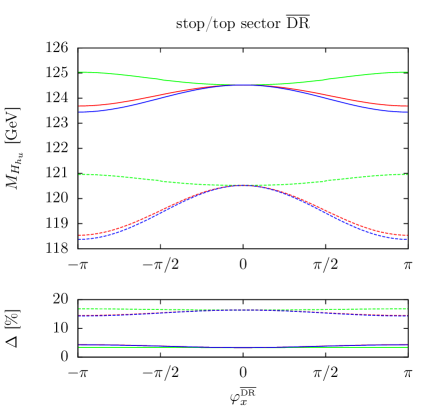
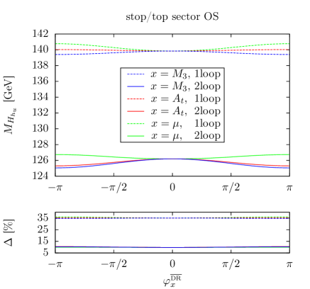
Figure 6: Upper Panels: One-loop (dashed line) and two-loop (solid line) mass of the SM-like Higgs boson as a function of the phases $\varphi_{\mu}$ (green/grey), $\varphi_{A_{t}}$ (red/black upper) and $\varphi_{M_{3}}$ (blue/black lower). Lower Panels: Size of the relative correction of $n^{th}$ order to the mass of the SM-like Higgs boson with respect to the $(n-1)^{st}$ order – i.e. $\Delta=|M_{H_{h_{u}}}^{(n)}-M_{H_{h_{u}}}^{(n-1)}|/M_{H_{h_{u}}}^{(n-1)}$ – in percent as a function of the phases $\varphi_{\mu}$ (green/grey), $\varphi_{A_{t}}$ (red) and $\varphi_{M_{3}}$ (blue) for $n=2$ (solid line) and $n=1$ (dashed line). On the left-hand side $\overline{\text{DR}}$ renormalization was employed in the top/stop sector and OS renormalization on the right-hand side.

Figure 6 shows the dependence of the one- and two-loop corrections to the mass of the $h_{u}$-like Higgs boson on the phases $\varphi_{A_{t}}$, $\varphi_{M_{3}}$ and $\varphi_{\mu}$ for the $\overline{\text{DR}}$ renormalization scheme as well as for the OS scheme in the top/stop sector. We start from the above defined parameter point and turn on separately one of the three phases. The corrections are displayed only for the $h_{u}$-like Higgs boson, because it is affected the strongest by the ${\cal O}(\alpha_{t}\alpha_{s})$ corrections. For both schemes the phase dependence displayed at two-loop level is very similar. For the here investigated scenario the strongest dependence occurs for the variation of the phase of $M_{3}$. The dependence on $\varphi_{A_{t}}$ is slightly less pronounced, but comparable, whereas the curve for $\varphi_{\mu}$ is significantly flatter. We have taken care to vary $\varphi_{\mu}$ in such a way that the CP-violating phase, which appears already at tree level in the Higgs sector, i.e. $\varphi_{y}=\varphi_{\kappa}-\varphi_{\lambda}+2\varphi_{s}-\varphi_{u}$, remains at zero. This implies that $\varphi_{\lambda}$ and $\varphi_{s}$ were varied at the same time, in particular $\varphi_{\lambda}=2\varphi_{s}=2/3\varphi_{\mu}$. The phases $\varphi_{\kappa}$ and $\varphi_{u}$ are kept zero. The correlation, respectively, anticorrelation of the dependences of the loop corrections on the various phases can be traced back to the observation, that the influence of the phases $\varphi_{M_{3}}$, $\varphi_{A_{t}}$ and $\varphi_{\mu}$ can be described by two independent phase combinations $\varphi_{1}$ and $\varphi_{2}$ given by

$$\varphi_{1}=\varphi_{\mu}+\varphi_{A_{t}}\qquad\mbox{ and }\qquad\varphi_{2}=\varphi_{M_{3}}-\varphi_{A_{t}}\;.$$ (4.83)

The relative influence of $\varphi_{1,2}$ on the loop corrections can then explain the observed behaviour.

At the one-loop level the results for the two different renormalization schemes in the top/stop sector seem quite different at first sight. However, it has to be kept in mind, that in the $\overline{\text{DR}}$ scheme the OS input value for the top mass has to be converted to the $\overline{\text{DR}}$ top mass and while doing so the finite counterterm to the top mass, which in the OS scheme is included in the two-loop calculation, is already induced at one-loop level in the value of the $\overline{\text{DR}}$ mass. Therefore some corrections of order ${\cal O}(\alpha_{t}\alpha_{s})$, which in the OS scheme only appear at the two-loop level, are moved to the one-loop level. This is also the reason why the loop-corrected masses in the $\overline{\text{DR}}$ scheme show a dependence on the phase $\varphi_{M_{3}}$ already at the one-loop level, although genuine diagrammatic gluino corrections only appear at two-loop level. For the OS scheme this dependence at one-loop level is due to the conversion of $A_{t}$ and of the soft SUSY breaking masses, which in the SLHA input are $\overline{\text{DR}}$ parameters, to the OS scheme. The lower panels of Fig. 6 display the relative loop corrections of $n$-loop order compared to the one at $(n-1)$-loop order ($n=1,2$),

$$\Delta=\frac{|M_{H_{h_{u}}}^{(n)}-M_{H_{h_{u}}}^{(n-1)}|}{M_{H_{h_{u}}}^{(n-1)}}\;.$$ (4.84)

As can be read off from the plots, the two-loop corrections relative to the one-loop mass are of course smaller than the one-loop corrections relative to the tree-level mass, which amount to about 15% in the $\overline{\text{DR}}$ scheme and to about 35% when adopting OS renormalization. Still the two-loop corrections amount to some $5-10\%$. (In the left lower panel, the lines for the $\varphi_{M_{3}}$ and the $\varphi_{A_{t}}$ dependence lie on top of each other, whereas in the right lower panel all lines lie nearly on top of each other at the respective loop order.)

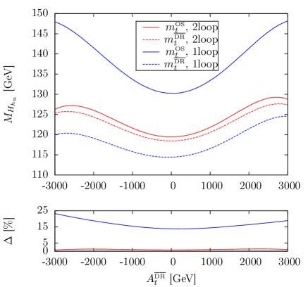
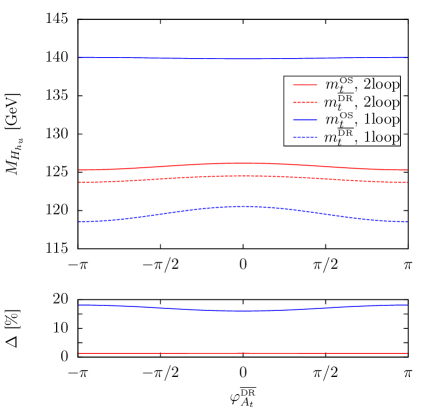
Figure 7: Upper Panel: Mass of the $h_{u}$-like Higgs boson as a function of $A_{t}^{\overline{\text{DR}}}$ (left) and $\varphi_{A_{t}}^{\overline{\text{DR}}}$ (right) including only one loop corrections (blue/two outer lines) and including also two loop corrections (red/two middle lines). For the renormalization of the top and stop sector either an OS scheme (solid line) or a $\overline{\text{DR}}$ scheme (dashed line) is applied. Lower Panel: Absolute value of the relative deviation of the result using OS renormalization in the top and stop sector with respect to the result using a $\overline{\text{DR}}$ scheme – i.e. $\Delta=|M_{H_{h_{u}}}^{m_{t}(\overline{\text{DR}})}-M_{H_{h_{u}}}^{m_{t}({\tiny\mbox{OS}})}|/M_{H_{h_{u}}}^{m_{t}({\tiny\overline{\text{DR}}})}$ – in percent as a function of $A_{t}^{\overline{\text{DR}}}$ (left) and $\varphi_{A_{t}}^{\overline{\text{DR}}}$ at two (red/lower line) and one loop order (blue/upper line).

To provide a rough estimate of the theoretical error due to missing higher order corrections, Fig. 7 shows the one-loop and two-loop mass of the $h_{u}$-like Higgs boson as a function of the $\overline{\text{DR}}$ parameters $A_{t}$ (left) and $\varphi_{A_{t}}$ (right) for both $\overline{\text{DR}}$ and OS renormalization in the top/stop sector. The difference between the two schemes is more pronounced for large absolute values of $A_{t}$. As expected the difference in the masses obtained using the two schemes,

$$\Delta=\frac{|M_{H_{h_{u}}}^{m_{t}(\overline{\text{DR}})}-M_{H_{h_{u}}}^{m_{t}({\tiny\mbox{OS}})}|}{M_{H_{h_{u}}}^{m_{t}({\tiny\overline{\text{DR}}})}}\;,$$ (4.85)

becomes much smaller when going from one to two loops. The lower panels of Fig. 7 show that it drops from some $15-25\%$ difference to a value below $1.5\%$. This is an indicator that the theoretical error is also reduced. The convergence in the $\overline{\text{DR}}$ scheme is better than in the OS scheme.

Note, that the one-loop corrections in the OS top mass scheme are symmetric with respect to a change of $A_{t}$, while this is not the case for the $\overline{\text{DR}}$ scheme. This is due to the threshold effects in the conversion of the top OS to $\overline{\text{DR}}$ mass. They depend on the sign of $A_{t}$. In the right plot, the variation of the loop-corrected masses with $\varphi_{A_{t}}$ is due to two effects, the genuine dependence on the phase and the change of the stop mass values with the phase, where the latter is the dominant effect.

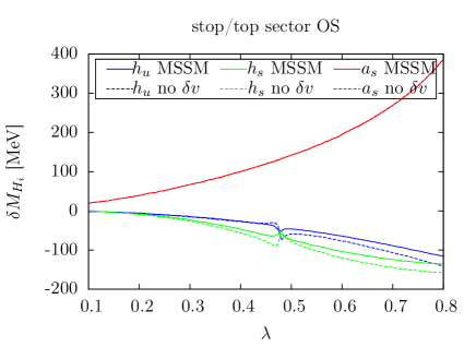
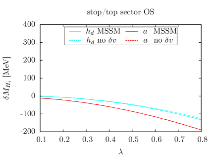
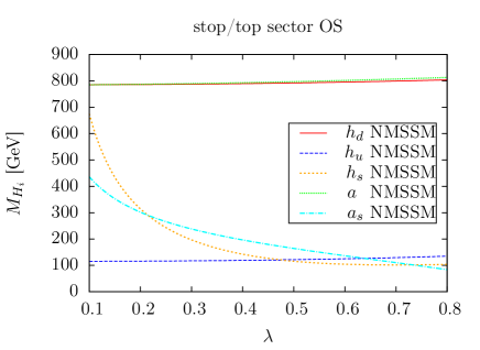
Figure 8: Upper plots: The solid lines show the absolute difference of the Higgs boson masses obtained when using only the MSSM-like ${\cal O}(\alpha_{t}\alpha_{s})$ corrections to the masses and when including the NMSSM specific $\alpha_{t}\alpha_{s}$; the dotted lines show the absolute difference of the masses obtained when neglecting the finite part of the two-loop $\delta^{\text{\tiny(}\!\text{\tiny 2}\!\text{\tiny)}}\!v/v$ term and when performing the full NMSSM ${\cal O}(\alpha_{t}\alpha_{s})$ calculation. Left: for the $h_{u}$ (blue/black lower lines), $h_{s}$ (green/grey lower lines) and $a_{s}$ (red/black upper lines) dominated states. Right: for the $h_{d}$ (light blue/grey lines) and $a$ (red/black lines) dominated heavy Higgs bosons. Lower: Higgs boson masses for the complete ${\cal O}(\alpha_{t}\alpha_{s})$ NMSSM corrections. All plots as a function of $\lambda$.

In Figure 8 (upper part) we illustrate the impact of the $\delta^{\text{\tiny(}\!\text{\tiny 2}\!\text{\tiny)}}\!v/v$ contribution, that only in the NMSSM contributes to the Higgs boson masses at order ${\cal O}(\alpha_{t}\alpha_{s})$, and of the genuine contributions from the singlet-doublet mixing. In particular this means that in the two-loop corrections to the Higgs boson masses we have turned off the finite part of the $\delta^{\text{\tiny(}\!\text{\tiny 2}\!\text{\tiny)}}\!v/v$ contribution in the approximation labeled ’no $\delta v$’, and in the approximation ’MSSM’ we have taken the MSSM limit for the two-loop corrections as specified at the end of subsection 2.1. As renormalization scheme we have chosen the OS scheme here. The plots show the absolute difference in the two-loop corrected mass values for both approximations as a function of $\lambda$. For illustrative purposes we allow to vary $\lambda$ here beyond the perturbativity limit, which is roughly given by $\sqrt{\lambda^{2}+\kappa^{2}}<0.7$. While the overall effect is small and below 1 GeV, it can easily be seen that the importance of the neglected contributions rises with $\lambda$, as expected. For small values of $\lambda$ the masses are very close to those obtained when using only the MSSM two-loop corrections. Regarding the impact of the finite part of the $\delta^{\text{\tiny(}\!\text{\tiny 2}\!\text{\tiny)}}\!v/v$ term it is interesting to note that neglecting it in the two-loop counterterm mass matrix leads to nearly the same result (the lines lie on top of each other) for the pseudoscalar masses as obtained in the MSSM limit of the two-loop corrections, where this term vanishes anyway. Another interesting observation is that it is also possible to be further away from the full result when neglecting the $\delta^{\text{\tiny(}\!\text{\tiny 2}\!\text{\tiny)}}\!v/v$ contribution than when simply using the MSSM contributions. This is the case for the Higgs bosons that are dominated by the up-type or by the singlet component, i.e. for the $h_{u}$ and $h_{s}$-like Higgs bosons. The lower plot in Fig. 8 displays the values of the two-loop corrected Higgs boson masses. The lines for the heavy $a$ and $h_{d}$ dominated masses lie on top of each other. The plot also shows the cross-over of the $h_{u}$ and $h_{s}$-like Higgs boson masses at $\lambda\approx 0.475$. There is another cross-over with the $a_{s}$-like Higgs boson. However, as we set all phases to zero in this plot, so that there is no CP mixing, this does not affect the CP-even light Higgs masses.

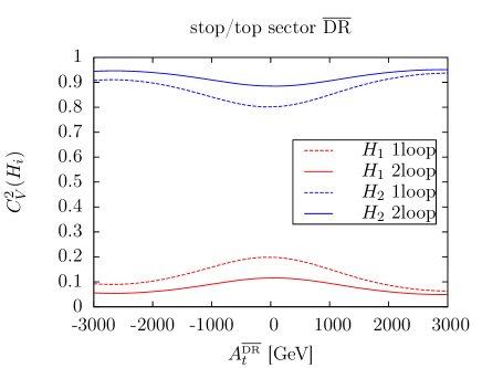
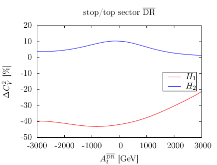
Figure 9: Left: Square of the coupling to vector bosons normalized to the respective SM coupling for the lightest (red/lower) and next-to-lightest Higgs boson (blue/upper) at one-loop order (dashed) and at two-loop order (solid). Right: Size of the two-loop correction to $C_{V}^{2}(H_{i})$ relative to the one-loop result for $H_{1}$ (red/lower) and $H_{2}$ (blue/upper); i.e. $\Delta C_{V}^{2}=[(C_{V}^{2})^{\text{(2loop)}}-(C_{V}^{2})^{\text{(1loop)}}]/(C_{V}^{2})^{\text{(1loop)}}$.

Another interesting question is how the mixing matrix elements are affected by non-vanishing complex phases. The matrix elements enter the Higgs couplings and hence influence the Higgs phenomenology. In general the mixing is hardly influenced by the phases, unless two of the Higgs bosons are almost mass degenerate and hence share their various doublet/singlet scalar/pseudoscalar contributions, as we explicitly verified. As in this case, however, it turns out that the mixing elements in the $p^{2}=0$ approximation differ substantially from the results obtained from the iterative procedure, also the mass values need to be obtained in the $p^{2}=0$ approximation to allow for a consistent interpretation of the mass values and their related mixing elements.

In Figs. 9 and 10 we show the influence of the loop corrections on the couplings $C_{V}$ to the vector bosons $V=W,Z$ and $C_{b}$ to the bottom quarks of the two lightest Higgs bosons, $H_{1}$ and $H_{2}$. The couplings are normalized to the corresponding SM couplings, so that $C_{V}$ reads ($i=1,2$)

$$C_{V}(H_{i})={\cal R}^{l}_{i1}\cos\beta+{\cal R}^{l}_{i2}\sin\beta\;,$$ (4.86)

where ${\cal R}^{l}_{ij}$ denote the matrix elements of the loop-corrected mixing matrix evaluated at zero external momentum, which at tree level has been defined in Eq. (2.10). The CP-even Higgs couplings to the bottom quarks are given by

$$C_{b}(H_{i})=\frac{{\cal R}^{l}_{i1}}{\cos\beta}\;.$$ (4.87)

In Fig. 9 (left) the couplings of $H_{1}$ and $H_{2}$ to the vector bosons are displayed at one- and two-loop level as a function of $A_{t}^{\overline{\text{DR}}}$. In the scenario considered here these are the only two Higgs bosons which couple non-negligibly to vector bosons. Since the scenario features a relatively small $\tan\beta$ value of $\sim 4$, the Higgs boson with the largest $h_{u}$ component and hence a sizeable ${\cal R}_{i2}^{l}$ has the largest coupling to vector bosons. Therefore the coupling of $H_{2}$ is around $\sim 0.9$, whereas the coupling of $H_{1}$, which is mainly singlet like is $\sim 0.1$. The right-hand side of Fig. 9 shows the relative correction ($x=V,b$)

$$\Delta C_{x}^{2}=\frac{(C_{x}^{2})^{\text{(2loop)}}-(C_{x}^{2})^{\text{(1loop)}}}{(C_{x}^{2})^{\text{(1loop)}}}$$ (4.88)

when going from one-loop to two-loop. Since the inclusion of the two-loop corrections changes the admixture of the different Higgs bosons, the coupling of $H_{1}$ to vector bosons is reduced, whereas the coupling of $H_{2}$ is increased. The relative corrections can be up to 40%. The couplings $C_{u}$ to the up-type quarks,

$$C_{u}(H_{i})=\frac{{\cal R}^{l}_{i2}}{\sin\beta}\;,$$ (4.89)

show almost the same behaviour so that we do not display the corresponding figures separately here. In both cases, the two-loop corrections render the SM-like Higgs boson even more SM-like.

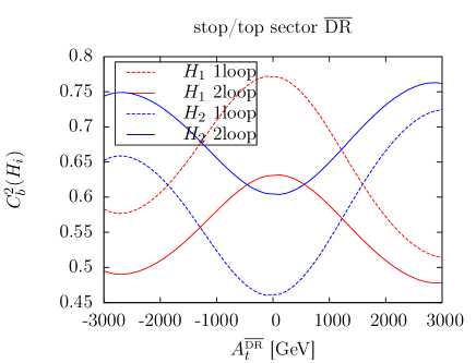
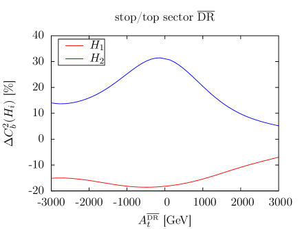
Figure 10: Same as Fig. 9, but for the coupling to bottom quarks.

Figure 10 is the analogous plot for the coupling to the bottom quarks. As $H_{1}$ has a non-negligible $h_{d}$ admixture, quantified by ${\cal R}^{l}_{i1}$, for the chosen $\tan\beta\approx 4$ its coupling to bottom quarks is significant. The two-loop corrections reduce this coupling by about 10-20%. The $h_{u}$-like $H_{2}$ couples with comparable strength to the down-type quarks at one-loop level, but at two-loop level the corrections increase the coupling by up to 30%. Figures 9 and 10 illustrate that the influence of the two-loop corrections on the couplings of the light Higgs bosons can be sizeable, which in turn leads to significant effects on the phenomenology of these Higgs bosons. This underlines the importance of including the two-loop corrections to the Higgs boson masses and mixing matrix elements for proper phenomenological investigations.

5 Conclusions

We have computed the two-loop corrections to the masses of the Higgs bosons in the CP-violating NMSSM at order ${\cal O}(\alpha_{t}\alpha_{s})$ using the Feynman diagrammatic approach with vanishing external momentum. The calculation is based on a mixed $\overline{\text{DR}}$-on-shell renormalization scheme. The corrections have been implemented in the Fortran package NMSSMCALC. The user has the choice between the default $\overline{\text{DR}}$ and an OS scheme for the renormalization of the top/stop sector. For the light Higgs boson masses, the corrections turn out to be important and are of the order of 5-10% for the SM-like Higgs boson, depending on the adopted top/stop renormalization scheme. The effect on its couplings to the vector bosons and to the top quarks is of the same order, with even larger corrections for the smaller bottom Yukawa couplings. To summarize, the two-loop corrections mainly affect the mass and the couplings of the $h_{u}$-dominated Higgs boson as well as the couplings of the light singlet-like Higgs state. For a proper interpretation of the experimental results and in order to make reliable theoretical predictions, two-loop corrections therefore have to be taken into account, in particular when investigating the phenomenology of the light Higgs bosons. The genuine NMSSM contributions at two-loop order turn out to be small for values of the singlet-doublet mixing coupling $\lambda$, that are still within the perturbativity limit.

An estimate of the remaining theoretical uncertainties due to missing higher order corrections, based on the variation of the renormalization scheme in the top/stop sector, shows, that the uncertainty is reduced when going from one- to two-loop order. The difference in the mass values of the SM-like Higgs boson for the two schemes decreases from 15-25% to below 1.5%.

We have not considered yet the ${\cal O}(\alpha_{b}\alpha_{s})$ contribution in the two-loop corrections. It is small for small values of $\tan\beta$, as chosen here and as favoured by the NMSSM. We plan to include the ${\cal O}(\alpha_{b}\alpha_{s})$ correction in future work.

Acknowledgments

DTN (in part), MMM and KW are supported by the DFG SFB/TR9 “Computational Particle Physics”. DTN thanks the Institute for Theoretical Physics at the Karlsruhe Institute of Technology for hospitality where part of this work has been performed. We are grateful to Pietro Slavich and Dominik Stöckinger for discussions.

Appendix

Appendix A The running $\overline{\text{DR}}$ top mass

Using as input the top quark pole mass $M_{t}$, we first translate it to the running $\overline{\text{MS}}$ top mass $m^{\overline{\text{MS}}}_{t}(M_{t})$ by applying the two-loop relation, see e.g. [147] and references therein,

$$m^{\overline{\text{MS}}}_{t}(M_{t})=\left(1-\frac{4}{3}\left(\frac{\alpha_{s}(M_{t})}{\pi}\right)-9.1253\left(\frac{\alpha_{s}(M_{t})}{\pi}\right)^{2}\right)M_{t}\;,$$ (A.90)

where $\alpha_{s}$ is the strong coupling constant at two-loop order. Then $m^{\overline{\text{MS}}}_{t}(M_{t})$ is evolved up to the renormalization scale $\mu_{R}$, by using the two-loop formula

$$m_{t}^{\overline{\text{MS}}}(\mu_{R})=U_{6}(\mu_{R},M_{t})m^{\overline{\text{MS}}}_{t}(M_{t})\hskip 8.53581pt\;\mbox{for}\;\mu_{R}>M_{t}\;,$$ (A.91)

where the evolution factor $U_{n}$ reads (see e.g. [148])

$$U_{n}(Q_{2},Q_{1}) = \left(\frac{\alpha_{s}(Q_{2})}{\alpha_{s}(Q_{1})}\right)^{d_{n}}\left[1+\frac{\alpha_{s}(Q_{1})-\alpha_{s}(Q_{2})}{4\pi}J_{n}\right]\;,\hskip 8.53581ptQ_{2}>Q_{1}$$ (A.92)

$$d_{n} = \frac{12}{33-2n}\;,\hskip 8.53581ptJ_{n}=-\frac{8982-504n+40n^{2}}{3(33-2n)^{2}}\;,$$

with $n=6$ for $Q>M_{t}$. From the $\overline{\text{MS}}$ masses the $\overline{\text{DR}}$ masses are computed at the SUSY scale, i.e. $\mu_{R}=M_{\text{SUSY}}$, by using the two-loop relation [149, 150, 151],

$$m_{t}^{\overline{\text{DR}},\text{SM}}(M_{\text{SUSY}})=m_{t}^{\overline{\text{MS}}}(M_{\text{SUSY}})\left[1-\frac{\alpha_{s}(M_{\text{SUSY}})}{3\pi}-\frac{\alpha_{s}^{2}(M_{\text{SUSY}})}{144\pi^{2}}(73-3n)\right]\;.$$ (A.93)

The $\overline{\text{DR}}$ supersymmetric top mass is then calculated from the $\overline{\text{DR}}$ SM top mass as,

$$m_{t}^{\overline{\text{DR}},\text{NMSSM}}=m_{t}^{\overline{\text{DR}},\text{SM}}(M_{\text{SUSY}})+dm_{t}\,,$$ (A.94)

where

$$dm_{t}= \frac{\alpha_{s}(M_{\text{SUSY}})}{6\pi}\Big{[}-2m_{t}\text{Re}\Big{(}B_{1}(m_{t}^{2},m_{\tilde{g}}^{2},m_{\tilde{t}_{1}}^{2})+B_{1}(m_{t}^{2},m_{\tilde{g}}^{2},m_{\tilde{t}_{2}}^{2})$$ (A.95)

$$+2m_{\tilde{g}}\text{Re}\left(B_{0}(m_{t}^{2},m_{\tilde{g}}^{2},m_{\tilde{t}_{1}}^{2})-B_{0}(m_{t}^{2},m_{\tilde{g}}^{2},m_{\tilde{t}_{2}}^{2})\right)$$

$$\times(e^{i(\varphi_{3}+\varphi_{u})}\mathcal{U}_{\tilde{t}_{22}}\mathcal{U}_{\tilde{t}_{21}}^{*}+e^{-i(\varphi_{3}+\varphi_{u})}\mathcal{U}_{\tilde{t}_{21}}\mathcal{U}_{\tilde{t}_{22}}^{*})\Big{]}\,.$$

Here the $\overline{\text{DR}}$ top mass at the SUSY-scale has to be used, i.e. $m_{t}=m_{t}^{\overline{\text{DR}}}(M_{\text{SUSY}})$. For the scalar two-point function $B_{0}(p^{2},m_{1}^{2},m_{2}^{2})$ we use the convention

$$B_{0}(p^{2},m_{1}^{2},m_{2}^{2})=16\pi^{2}\mu_{R}^{4-D}\int\frac{d^{D}q}{i(2\pi)^{D}}\frac{1}{(q^{2}-m_{1}^{2})((q-p)^{2}-m_{2}^{2})}\;.$$ (A.96)

The two-point tensor integral of rank one $B_{1}(p^{2},m_{1}^{2},m_{2}^{2})$, can be written in terms of scalar one-point and two-point functions as

$$B_{1}(p^{2},m_{1}^{2},m_{2}^{2})=\frac{1}{2p^{2}}\Big{[}A_{0}(m_{1}^{2})-A_{0}(m_{2}^{2})-(p^{2}-m_{2}^{2}+m_{1}^{2})B_{0}(p^{2},m_{1}^{2},m_{2}^{2})\Big{]}\;,$$ (A.97)

where the convention for $A_{0}$ is

$$A_{0}(m^{2})=16\pi^{2}\mu_{R}^{4-D}\int\frac{d^{D}q}{i(2\pi)^{D}}\frac{1}{(q^{2}-m^{2})}\;.$$ (A.98)

Appendix B Counterterm Mass Matrix

The $\overline{\text{DR}}$ counterterms for $|\lambda|$ and $\tan\beta$ and furthermore the divergent parts of the OS counterterms $\delta^{\text{\tiny(}\!\text{\tiny 2}\!\text{\tiny)}}\!v$ and $\delta M_{H^{\pm}}^{2}$ are related to the counterterm of the field renormalization constant $\delta^{\text{\tiny(}\!\text{\tiny 2}\!\text{\tiny)}}\!Z_{H_{u}}$ as already explained in Sec. 3.2. If these relations are inserted explicitly into the renormalized self-energy, it can be shown analytically that most of the $\delta^{\text{\tiny(}\!\text{\tiny 2}\!\text{\tiny)}}\!Z_{H_{u}}$ contributions from the counterterm mass matrix cancel against the field renormalization part of the renormalized self-energy and only one additional contribution in the $h_{d}h_{s}$ component is left. Hence, we give the explicit analytic form only for the part of the counterterm mass matrix of the neutral Higgs bosons at two-loop level that yields finite contributions, $\delta^{\text{\tiny(}\!\text{\tiny 2}\!\text{\tiny)}}\!\mathcal{M}_{hh}\big{|}^{\text{fin}}$, i.e. counterterms of $\overline{\text{DR}}$ parameters are dropped. Hence $\delta^{\text{\tiny(}\!\text{\tiny 2}\!\text{\tiny)}}\!\mathcal{M}_{hh}\big{|}^{\text{fin}}$ only depends on the two-loop counterterms $\delta^{\text{\tiny(}\!\text{\tiny 2}\!\text{\tiny)}}\!M_{H_{\pm}}^{2}$, $\delta^{\text{\tiny(}\!\text{\tiny 2}\!\text{\tiny)}}\!v$, $\delta^{\text{\tiny(}\!\text{\tiny 2}\!\text{\tiny)}}\!t_{h_{u}}$, $\delta^{\text{\tiny(}\!\text{\tiny 2}\!\text{\tiny)}}\!t_{h_{d}}$, $\delta^{\text{\tiny(}\!\text{\tiny 2}\!\text{\tiny)}}\!t_{h_{s}}$, $\delta^{\text{\tiny(}\!\text{\tiny 2}\!\text{\tiny)}}\!t_{a_{d}}$ and $\delta^{\text{\tiny(}\!\text{\tiny 2}\!\text{\tiny)}}\!t_{a_{s}}$ as defined in Sec. 3.2. The counterterm mass matrix is given in the basis $(h_{d},h_{u},h_{s},a,a_{s})$.

$$\delta^{\text{\tiny(}\!\text{\tiny 2}\!\text{\tiny)}}\!\mathcal{M}_{hh}\big{|}^{\text{fin}}_{h_{d}h_{d}}= \delta^{\text{\tiny(}\!\text{\tiny 2}\!\text{\tiny)}}\!v\,v|\lambda|^{2}\sin^{2}\!\beta+\delta^{\text{\tiny(}\!\text{\tiny 2}\!\text{\tiny)}}\!M_{H^{\pm}}^{2}\sin^{2}\!\beta$$

$$+\frac{\delta^{\text{\tiny(}\!\text{\tiny 2}\!\text{\tiny)}}\!t_{h_{d}}\left(1-\sin^{4}\!\beta\right)}{v\cos\!\beta}-\frac{\delta^{\text{\tiny(}\!\text{\tiny 2}\!\text{\tiny)}}\!t_{h_{u}}\sin\!\beta\cos^{2}\!\beta}{v}\,,$$ (B.99)

$$\delta^{\text{\tiny(}\!\text{\tiny 2}\!\text{\tiny)}}\!\mathcal{M}_{hh}\big{|}^{\text{fin}}_{h_{d}h_{u}}= \delta^{\text{\tiny(}\!\text{\tiny 2}\!\text{\tiny)}}\!v\,v|\lambda|^{2}\sin\!\beta\cos\!\beta-\delta^{\text{\tiny(}\!\text{\tiny 2}\!\text{\tiny)}}\!M_{H^{\pm}}^{2}\sin\!\beta\cos\!\beta+\frac{\delta^{\text{\tiny(}\!\text{\tiny 2}\!\text{\tiny)}}\!t_{h_{d}}\sin^{3}\!\beta}{v}+\frac{\delta^{\text{\tiny(}\!\text{\tiny 2}\!\text{\tiny)}}\!t_{h_{u}}\cos^{3}\!\beta}{v}\,,$$ (B.100)

$$\delta^{\text{\tiny(}\!\text{\tiny 2}\!\text{\tiny)}}\!\mathcal{M}_{hh}\big{|}^{\text{fin}}_{h_{d}h_{s}}= \frac{\delta^{\text{\tiny(}\!\text{\tiny 2}\!\text{\tiny)}}\!v\,\left(|\lambda|^{2}\cos\!\beta\left(2v_{s}^{2}-3v^{2}\sin^{2}\!\beta\right)-\sin\!\beta\left(v_{s}^{2}|\kappa||\lambda|\cos\varphi_{y}+\sin\!2\beta\,M_{H^{\pm}}^{2}\right)\right)}{2v_{s}}$$

$$\quad-\frac{\delta^{\text{\tiny(}\!\text{\tiny 2}\!\text{\tiny)}}\!M_{H^{\pm}}^{2}v\sin^{2}\!\beta\cos\!\beta}{v_{s}}+\frac{\delta^{\text{\tiny(}\!\text{\tiny 2}\!\text{\tiny)}}\!t_{h_{d}}\sin^{4}\!\beta}{v_{s}}+\frac{\delta^{\text{\tiny(}\!\text{\tiny 2}\!\text{\tiny)}}\!t_{h_{u}}\sin\!\beta\cos^{3}\!\beta}{v_{s}}\,,$$ (B.101)

$$\delta^{\text{\tiny(}\!\text{\tiny 2}\!\text{\tiny)}}\!\mathcal{M}_{hh}\big{|}^{\text{fin}}_{h_{d}a\,}= \frac{\delta^{\text{\tiny(}\!\text{\tiny 2}\!\text{\tiny)}}\!t_{a_{d}}}{v\tan\!\beta}\,,$$ (B.102)

$$\delta^{\text{\tiny(}\!\text{\tiny 2}\!\text{\tiny)}}\!\mathcal{M}_{hh}\big{|}^{\text{fin}}_{h_{d}a_{s}}= \frac{\delta^{\text{\tiny(}\!\text{\tiny 2}\!\text{\tiny)}}\!t_{a_{d}}}{v_{s}}-\frac{3}{2}\delta^{\text{\tiny(}\!\text{\tiny 2}\!\text{\tiny)}}\!v\,v_{s}|\kappa||\lambda|\sin\!\beta\sin\varphi_{y}\,,$$ (B.103)

$$\delta^{\text{\tiny(}\!\text{\tiny 2}\!\text{\tiny)}}\!\mathcal{M}_{hh}\big{|}^{\text{fin}}_{h_{u}h_{u}}= \delta^{\text{\tiny(}\!\text{\tiny 2}\!\text{\tiny)}}\!v\,v|\lambda|^{2}\cos^{2}\!\beta+\delta^{\text{\tiny(}\!\text{\tiny 2}\!\text{\tiny)}}\!M_{H^{\pm}}^{2}\cos^{2}\!\beta$$

$$\quad-\frac{\delta^{\text{\tiny(}\!\text{\tiny 2}\!\text{\tiny)}}\!t_{h_{d}}\sin^{2}\!\beta\cos\!\beta}{v}+\frac{\delta^{\text{\tiny(}\!\text{\tiny 2}\!\text{\tiny)}}\!t_{h_{u}}(5\sin\!\beta+\sin 3\beta)}{4v}\,,$$ (B.104)

$$\delta^{\text{\tiny(}\!\text{\tiny 2}\!\text{\tiny)}}\!\mathcal{M}_{hh}\big{|}^{\text{fin}}_{h_{u}h_{s}}= \frac{\delta^{\text{\tiny(}\!\text{\tiny 2}\!\text{\tiny)}}\!v\,\left(\sin\!\beta\left(|\lambda|^{2}\left(2v_{s}^{2}-3v^{2}\cos^{2}\!\beta\right)-2\cos^{2}\!\beta M_{H^{\pm}}^{2}\right)-v_{s}^{2}|\kappa||\lambda|\cos\!\beta\cos\varphi_{y}\right)}{2v_{s}}$$

$$-\frac{\delta^{\text{\tiny(}\!\text{\tiny 2}\!\text{\tiny)}}\!M_{H^{\pm}}^{2}v\sin\!\beta\cos^{2}\!\beta}{v_{s}}+\frac{\delta^{\text{\tiny(}\!\text{\tiny 2}\!\text{\tiny)}}\!t_{h_{d}}\sin^{3}\!\beta\cos\!\beta}{v_{s}}+\frac{\delta^{\text{\tiny(}\!\text{\tiny 2}\!\text{\tiny)}}\!t_{h_{u}}\cos^{4}\!\beta}{v_{s}}\,,$$ (B.105)

$$\delta^{\text{\tiny(}\!\text{\tiny 2}\!\text{\tiny)}}\!\mathcal{M}_{hh}\big{|}^{\text{fin}}_{h_{u}a\,}= \frac{\delta^{\text{\tiny(}\!\text{\tiny 2}\!\text{\tiny)}}\!t_{a_{d}}}{v}\,,$$ (B.106)

$$\delta^{\text{\tiny(}\!\text{\tiny 2}\!\text{\tiny)}}\!\mathcal{M}_{hh}\big{|}^{\text{fin}}_{h_{u}a_{s}}= \frac{\delta^{\text{\tiny(}\!\text{\tiny 2}\!\text{\tiny)}}\!t_{a_{d}}}{v_{s}\tan\!\beta}-\frac{3}{2}\delta^{\text{\tiny(}\!\text{\tiny 2}\!\text{\tiny)}}\!v\,v_{s}|\kappa||\lambda|\cos\!\beta\sin\varphi_{y}\,,$$ (B.107)

$$\delta^{\text{\tiny(}\!\text{\tiny 2}\!\text{\tiny)}}\!\mathcal{M}_{hh}\big{|}^{\text{fin}}_{h_{s}h_{s}}= \frac{\delta^{\text{\tiny(}\!\text{\tiny 2}\!\text{\tiny)}}\!vv}{2v_{s}^{2}}\Big{(}\sin^{2}\!2\beta\big{(}v^{2}|\lambda|^{2}+M_{H^{\pm}}^{2}\big{)}+v_{s}^{2}|\kappa||\lambda|\big{(}3\sin\!2\beta\sin\varphi_{y}\tan\!\left(\varphi_{\kappa}+3\varphi_{s}\right)$$

$$-2\sin\!\beta\cos\!\beta\cos\varphi_{y}\big{)}\Big{)}+\frac{\delta^{\text{\tiny(}\!\text{\tiny 2}\!\text{\tiny)}}\!M_{H^{\pm}}^{2}v^{2}\sin^{2}\!\beta\cos^{2}\!\beta}{v_{s}^{2}}$$

$$-\frac{\delta^{\text{\tiny(}\!\text{\tiny 2}\!\text{\tiny)}}\!t_{a_{d}}v\cos\!\beta\tan\!\left(\varphi_{\kappa}+3\varphi_{s}\right)}{v_{s}^{2}}+\frac{\delta^{\text{\tiny(}\!\text{\tiny 2}\!\text{\tiny)}}\!t_{a_{s}}\tan\!\left(\varphi_{\kappa}+3\varphi_{s}\right)}{v_{s}}$$

$$-\frac{\delta^{\text{\tiny(}\!\text{\tiny 2}\!\text{\tiny)}}\!t_{h_{d}}v\sin^{4}\!\beta\cos\!\beta}{v_{s}^{2}}+\frac{\delta^{\text{\tiny(}\!\text{\tiny 2}\!\text{\tiny)}}\!t_{h_{s}}}{v_{s}}-\frac{\delta^{\text{\tiny(}\!\text{\tiny 2}\!\text{\tiny)}}\!t_{h_{u}}v\sin\!\beta\cos^{4}\!\beta}{v_{s}^{2}}\,,$$ (B.108)

$$\delta^{\text{\tiny(}\!\text{\tiny 2}\!\text{\tiny)}}\!\mathcal{M}_{hh}\big{|}^{\text{fin}}_{h_{s}a}= \frac{1}{2}\delta^{\text{\tiny(}\!\text{\tiny 2}\!\text{\tiny)}}\!v\,v_{s}|\kappa||\lambda|\sin\varphi_{y}+\frac{\delta^{\text{\tiny(}\!\text{\tiny 2}\!\text{\tiny)}}\!t_{a_{d}}}{v_{s}\sin\!\beta}\,,$$ (B.109)

$$\delta^{\text{\tiny(}\!\text{\tiny 2}\!\text{\tiny)}}\!\mathcal{M}_{hh}\big{|}^{\text{fin}}_{h_{s}a_{s}}= 2\delta^{\text{\tiny(}\!\text{\tiny 2}\!\text{\tiny)}}\!v\,v|\kappa||\lambda|\sin\!2\beta\sin\varphi_{y}-\frac{2\delta^{\text{\tiny(}\!\text{\tiny 2}\!\text{\tiny)}}\!t_{a_{d}}v\cos\!\beta}{v_{s}^{2}}+\frac{2\delta^{\text{\tiny(}\!\text{\tiny 2}\!\text{\tiny)}}\!t_{a_{s}}}{v_{s}}\,,$$ (B.110)

$$\delta^{\text{\tiny(}\!\text{\tiny 2}\!\text{\tiny)}}\!\mathcal{M}_{hh}\big{|}^{\text{fin}}_{a\,a\,}= \delta^{\text{\tiny(}\!\text{\tiny 2}\!\text{\tiny)}}\!v\,v|\lambda|^{2}+\delta^{\text{\tiny(}\!\text{\tiny 2}\!\text{\tiny)}}\!M_{H^{\pm}}^{2}\,,$$ (B.111)

$$\delta^{\text{\tiny(}\!\text{\tiny 2}\!\text{\tiny)}}\!\mathcal{M}_{hh}\big{|}^{\text{fin}}_{a\,a_{s}}= \frac{\delta^{\text{\tiny(}\!\text{\tiny 2}\!\text{\tiny)}}\!v\,\left(\sin\!2\beta\left(3v^{2}|\lambda|^{2}+2M_{H^{\pm}}^{2}\right)-6v_{s}^{2}|\kappa||\lambda|\cos\varphi_{y}\right)}{4v_{s}}+\frac{\delta^{\text{\tiny(}\!\text{\tiny 2}\!\text{\tiny)}}\!M_{H^{\pm}}^{2}v\sin\!\beta\cos\!\beta}{v_{s}}$$

$$-\frac{\delta^{\text{\tiny(}\!\text{\tiny 2}\!\text{\tiny)}}\!t_{h_{d}}\sin^{3}\!\beta}{v_{s}}-\frac{\delta^{\text{\tiny(}\!\text{\tiny 2}\!\text{\tiny)}}\!t_{h_{u}}\cos^{3}\!\beta}{v_{s}}\,,$$ (B.112)

$$\delta^{\text{\tiny(}\!\text{\tiny 2}\!\text{\tiny)}}\!\mathcal{M}_{hh}\big{|}^{\text{fin}}_{a_{s}a_{s}}= \frac{\delta^{\text{\tiny(}\!\text{\tiny 2}\!\text{\tiny)}}\!vv\sin\!2\beta}{2v_{s}^{2}}\Big{(}\sin\!2\beta\big{(}v^{2}|\lambda|^{2}+M_{H^{\pm}}^{2}\big{)}$$

$$+3v_{s}^{2}|\kappa||\lambda|\big{(}\cos\varphi_{y}-3\sin\varphi_{y}\tan\left(\varphi_{\kappa}+3\varphi_{s}\right)\big{)}\Big{)}+\frac{\delta^{\text{\tiny(}\!\text{\tiny 2}\!\text{\tiny)}}\!M_{H^{\pm}}^{2}v^{2}\sin^{2}\!\beta\cos^{2}\!\beta}{v_{s}^{2}}$$

$$+\frac{3\delta^{\text{\tiny(}\!\text{\tiny 2}\!\text{\tiny)}}\!t_{a_{d}}v\cos\!\beta\tan\!\left(\varphi_{\kappa}+3\varphi_{s}\right)}{v_{s}^{2}}-\frac{3\delta^{\text{\tiny(}\!\text{\tiny 2}\!\text{\tiny)}}\!t_{a_{s}}\tan\!\left(\varphi_{\kappa}+3\varphi_{s}\right)}{v_{s}}$$

$$-\frac{\delta^{\text{\tiny(}\!\text{\tiny 2}\!\text{\tiny)}}\!t_{h_{d}}v\sin^{4}\!\beta\cos\!\beta}{v_{s}^{2}}+\frac{\delta^{\text{\tiny(}\!\text{\tiny 2}\!\text{\tiny)}}\!t_{h_{s}}}{v_{s}}-\frac{\delta^{\text{\tiny(}\!\text{\tiny 2}\!\text{\tiny)}}\!t_{h_{u}}v\sin\!\beta\cos^{4}\!\beta}{v_{s}^{2}}\,.$$ (B.113)

References

• [1] ATLAS Collaboration, G. Aad et al., Phys.Lett. B716, 1 (2012), 1207.7214.
• [2] CMS Collaboration, S. Chatrchyan et al., Phys.Lett. B716, 30 (2012), 1207.7235.
• [3] CMS Collaboration, (2013), CMS-PAS-SUS-13-009.
• [4] ATLAS Collaboration, G. Aad et al., (2014), 1407.0583.
• [5] ATLAS Collaboration, G. Aad et al., Phys.Rev. D90, 052008 (2014), 1407.0608.
• [6] C. Boehm, A. Djouadi, and Y. Mambrini, Phys.Rev. D61, 095006 (2000), hep-ph/9907428.
• [7] K.-i. Hikasa and M. Kobayashi, Phys.Rev. D36, 724 (1987).
• [8] M. Muhlleitner and E. Popenda, JHEP 1104, 095 (2011), 1102.5712.
• [9] R. Grober, M. Muhlleitner, E. Popenda, and A. Wlotzka, (2014), 1408.4662.
• [10] J. F. Gunion, H. E. Haber, G. L. Kane, and S. Dawson, Front.Phys. 80, 1 (2000).
• [11] S. P. Martin, Adv.Ser.Direct.High Energy Phys. 21, 1 (2010), hep-ph/9709356.
• [12] S. Dawson, p. 261 (1997), hep-ph/9712464.
• [13] A. Djouadi, Phys.Rept. 459, 1 (2008), hep-ph/0503173.
• [14] P. Fayet, Nucl.Phys. B90, 104 (1975).
• [15] R. Barbieri, S. Ferrara, and C. A. Savoy, Phys.Lett. B119, 343 (1982).
• [16] M. Dine, W. Fischler, and M. Srednicki, Phys.Lett. B104, 199 (1981).
• [17] H. P. Nilles, M. Srednicki, and D. Wyler, Phys.Lett. B120, 346 (1983).
• [18] J. Frere, D. Jones, and S. Raby, Nucl.Phys. B222, 11 (1983).
• [19] J. Derendinger and C. A. Savoy, Nucl.Phys. B237, 307 (1984).
• [20] J. R. Ellis, J. Gunion, H. E. Haber, L. Roszkowski, and F. Zwirner, Phys.Rev. D39, 844 (1989).
• [21] M. Drees, Int.J.Mod.Phys. A4, 3635 (1989).
• [22] U. Ellwanger, M. Rausch de Traubenberg, and C. A. Savoy, Phys.Lett. B315, 331 (1993), hep-ph/9307322.
• [23] U. Ellwanger, M. Rausch de Traubenberg, and C. A. Savoy, Z.Phys. C67, 665 (1995), hep-ph/9502206.
• [24] U. Ellwanger, M. Rausch de Traubenberg, and C. A. Savoy, Nucl.Phys. B492, 21 (1997), hep-ph/9611251.
• [25] T. Elliott, S. King, and P. White, Phys.Lett. B351, 213 (1995), hep-ph/9406303.
• [26] S. King and P. White, Phys.Rev. D52, 4183 (1995), hep-ph/9505326.
• [27] F. Franke and H. Fraas, Int.J.Mod.Phys. A12, 479 (1997), hep-ph/9512366.
• [28] M. Maniatis, Int.J.Mod.Phys. A25, 3505 (2010), 0906.0777.
• [29] U. Ellwanger, C. Hugonie, and A. M. Teixeira, Phys.Rept. 496, 1 (2010), 0910.1785.
• [30] S. King, M. Muhlleitner, and R. Nevzorov, Nucl.Phys. B860, 207 (2012), 1201.2671.
• [31] S. King, M. Muhlleitner, R. Nevzorov, and K. Walz, Nucl.Phys. B870, 323 (2013), 1211.5074.
• [32] U. Ellwanger, JHEP 1308, 077 (2013), 1306.5541.
• [33] S. Munir, Phys.Rev. D89, 095013 (2014), 1310.8129.
• [34] S. King, M. Muhlleitner, R. Nevzorov, and K. Walz, Phys.Rev. D90, 095014 (2014), 1408.1120.
• [35] N.-E. Bomark, S. Moretti, S. Munir, and L. Roszkowski, (2014), 1409.8393.
• [36] J. F. Gunion, Y. Jiang, and S. Kraml, Phys.Rev. D86, 071702 (2012), 1207.1545.
• [37] U. Ellwanger, Phys.Lett. B303, 271 (1993), hep-ph/9302224.
• [38] T. Elliott, S. King, and P. White, Phys.Lett. B305, 71 (1993), hep-ph/9302202.
• [39] T. Elliott, S. King, and P. White, Phys.Lett. B314, 56 (1993), hep-ph/9305282.
• [40] T. Elliott, S. King, and P. White, Phys.Rev. D49, 2435 (1994), hep-ph/9308309.
• [41] P. Pandita, Z.Phys. C59, 575 (1993).
• [42] U. Ellwanger and C. Hugonie, Phys.Lett. B623, 93 (2005), hep-ph/0504269.
• [43] G. Degrassi and P. Slavich, Nucl.Phys. B825, 119 (2010), 0907.4682.
• [44] F. Staub, W. Porod, and B. Herrmann, JHEP 1010, 040 (2010), 1007.4049.
• [45] M. D. Goodsell, K. Nickel, and F. Staub, (2014), 1411.4665.
• [46] K. Ender, T. Graf, M. Muhlleitner, and H. Rzehak, Phys.Rev. D85, 075024 (2012), 1111.4952.
• [47] D. T. Nhung, M. Muhlleitner, J. Streicher, and K. Walz, JHEP 1311, 181 (2013), 1306.3926.
• [48] S. Ham, J. Kim, S. Oh, and D. Son, Phys.Rev. D64, 035007 (2001), hep-ph/0104144.
• [49] S. Ham, S. Oh, and D. Son, Phys.Rev. D65, 075004 (2002), hep-ph/0110052.
• [50] S. Ham, Y. Jeong, and S. Oh, (2003), hep-ph/0308264.
• [51] K. Funakubo and S. Tao, Prog.Theor.Phys. 113, 821 (2005), hep-ph/0409294.
• [52] S. Ham, S. Kim, S. OH, and D. Son, Phys.Rev. D76, 115013 (2007), 0708.2755.
• [53] K. Cheung, T.-J. Hou, J. S. Lee, and E. Senaha, Phys.Rev. D82, 075007 (2010), 1006.1458.
• [54] T. Graf, R. Grober, M. Muhlleitner, H. Rzehak, and K. Walz, JHEP 1210, 122 (2012), 1206.6806.
• [55] U. Ellwanger, J. F. Gunion, and C. Hugonie, JHEP 0502, 066 (2005), hep-ph/0406215.
• [56] U. Ellwanger and C. Hugonie, Comput.Phys.Commun. 175, 290 (2006), hep-ph/0508022.
• [57] U. Ellwanger and C. Hugonie, Comput.Phys.Commun. 177, 399 (2007), hep-ph/0612134.
• [58] B. Allanach, Comput.Phys.Commun. 143, 305 (2002), hep-ph/0104145.
• [59] B. Allanach, P. Athron, L. C. Tunstall, A. Voigt, and A. Williams, Comput.Phys.Commun. 185, 2322 (2014), 1311.7659.
• [60] F. Staub, Comput.Phys.Commun. 182, 808 (2011), 1002.0840.
• [61] F. Staub, Computer Physics Communications 184, pp. 1792 (2013), 1207.0906.
• [62] F. Staub, Comput.Phys.Commun. 185, 1773 (2014), 1309.7223.
• [63] M. D. Goodsell, K. Nickel, and F. Staub, (2014), 1411.0675.
• [64] W. Porod, Comput.Phys.Commun. 153, 275 (2003), hep-ph/0301101.
• [65] W. Porod and F. Staub, Comput.Phys.Commun. 183, 2458 (2012), 1104.1573.
• [66] P. Athron, J.-h. Park, D. St ckinger, and A. Voigt, (2014), 1406.2319.
• [67] P. Athron, J.-h. Park, D. St ckinger, and A. Voigt, (2014), 1410.7385.
• [68] J. Baglio et al., EPJ Web Conf. 49, 12001 (2013).
• [69] J. Baglio et al., Comput.Phys.Commun. 185, 3372 (2014), 1312.4788.
• [70] M. Kobayashi and T. Maskawa, Prog.Theor.Phys. 49, 652 (1973).
• [71] P. Z. Skands et al., JHEP 0407, 036 (2004), hep-ph/0311123.
• [72] B. Allanach et al., Comput.Phys.Commun. 180, 8 (2009), 0801.0045.
• [73] S. Heinemeyer, W. Hollik, H. Rzehak, and G. Weiglein, Phys.Lett. B652, 300 (2007), 0705.0746.
• [74] S. Heinemeyer, H. Rzehak, and C. Schappacher, Phys.Rev. D82, 075010 (2010), 1007.0689.
• [75] G. ’t Hooft and M. Veltman, Nucl.Phys. B153, 365 (1979).
• [76] U. Nierste, D. Muller, and M. Bohm, Z.Phys. C57, 605 (1993).
• [77] A. I. Davydychev and J. Tausk, Nucl.Phys. B397, 123 (1993).
• [78] C. Ford, I. Jack, and D. Jones, Nucl.Phys. B387, 373 (1992), hep-ph/0111190.
• [79] R. Scharf and J. Tausk, Nucl.Phys. B412, 523 (1994).
• [80] G. Weiglein, R. Scharf, and M. Bohm, Nucl.Phys. B416, 606 (1994), hep-ph/9310358.
• [81] F. A. Berends and J. Tausk, Nucl.Phys. B421, 456 (1994).
• [82] S. P. Martin, Phys.Rev. D65, 116003 (2002), hep-ph/0111209.
• [83] S. P. Martin and D. G. Robertson, Comput.Phys.Commun. 174, 133 (2006), hep-ph/0501132.
• [84] G. Degrassi, S. Di Vita, and P. Slavich, (2014), 1410.3432.
• [85] T. Hahn, Comput.Phys.Commun. 140, 418 (2001), hep-ph/0012260.
• [86] A. Djouadi and C. Verzegnassi, Phys.Lett. B195, 265 (1987).
• [87] A. Djouadi, Nuovo Cim. A100, 357 (1988).
• [88] A. Djouadi et al., Phys.Rev.Lett. 78, 3626 (1997), hep-ph/9612363.
• [89] A. Djouadi et al., Phys.Rev. D57, 4179 (1998), hep-ph/9710438.
• [90] M. Sperling, D. Stockinger, and A. Voigt, JHEP 1307, 132 (2013), 1305.1548.
• [91] M. Sperling, D. Stockinger, and A. Voigt, JHEP 1401, 068 (2014), 1310.7629.
• [92] A. Brignole, Phys.Lett. B281, 284 (1992).
• [93] P. H. Chankowski, S. Pokorski, and J. Rosiek, Phys.Lett. B286, 307 (1992).
• [94] P. H. Chankowski, S. Pokorski, and J. Rosiek, Nucl.Phys. B423, 437 (1994), hep-ph/9303309.
• [95] A. Dabelstein, Z.Phys. C67, 495 (1995), hep-ph/9409375.
• [96] A. Dabelstein, Nucl.Phys. B456, 25 (1995), hep-ph/9503443.
• [97] A. Freitas and D. Stockinger, Phys.Rev. D66, 095014 (2002), hep-ph/0205281.
• [98] J. Kublbeck, M. Bohm, and A. Denner, Comput.Phys.Commun. 60, 165 (1990).
• [99] F. Staub, Comput.Phys.Commun. 181, 1077 (2010), 0909.2863.
• [100] R. Mertig, M. Bohm, and A. Denner, Comput.Phys.Commun. 64, 345 (1991).
• [101] R. Mertig and R. Scharf, Comput.Phys.Commun. 111, 265 (1998), hep-ph/9801383.
• [102] O. Tarasov, Phys.Rev. D54, 6479 (1996), hep-th/9606018.
• [103] O. Tarasov, Nucl.Phys. B502, 455 (1997), hep-ph/9703319.
• [104] G. Weiglein, R. Mertig, R. Scharf, and M. Bohm, (1995).
• [105] W. Siegel, Phys.Lett. B84, 193 (1979).
• [106] D. Stockinger, JHEP 0503, 076 (2005), hep-ph/0503129.
• [107] W. Hollik and D. Stockinger, Phys.Lett. B634, 63 (2006), hep-ph/0509298.
• [108] P. Bechtle, O. Brein, S. Heinemeyer, G. Weiglein, and K. E. Williams, Comput.Phys.Commun. 181, 138 (2010), 0811.4169.
• [109] P. Bechtle, O. Brein, S. Heinemeyer, G. Weiglein, and K. E. Williams, Comput.Phys.Commun. 182, 2605 (2011), 1102.1898.
• [110] P. Bechtle et al., Eur.Phys.J. C74, 2693 (2014), 1311.0055.
• [111] P. Bechtle, S. Heinemeyer, O. St l, T. Stefaniak, and G. Weiglein, Eur.Phys.J. C74, 2711 (2014), 1305.1933.
• [112] T. Inami, T. Kubota, and Y. Okada, Z.Phys. C18, 69 (1983).
• [113] A. Djouadi, M. Spira, and P. Zerwas, Phys.Lett. B264, 440 (1991).
• [114] M. Spira, A. Djouadi, D. Graudenz, and P. Zerwas, Phys.Lett. B318, 347 (1993).
• [115] M. Spira, A. Djouadi, D. Graudenz, and P. Zerwas, Nucl.Phys. B453, 17 (1995), hep-ph/9504378.
• [116] M. Kramer, E. Laenen, and M. Spira, Nucl.Phys. B511, 523 (1998), hep-ph/9611272.
• [117] K. Chetyrkin, B. A. Kniehl, and M. Steinhauser, Phys.Rev.Lett. 79, 353 (1997), hep-ph/9705240.
• [118] K. Chetyrkin, B. A. Kniehl, and M. Steinhauser, Nucl.Phys. B510, 61 (1998), hep-ph/9708255.
• [119] Y. Schroder and M. Steinhauser, JHEP 0601, 051 (2006), hep-ph/0512058.
• [120] K. Chetyrkin, J. H. Kuhn, and C. Sturm, Nucl.Phys. B744, 121 (2006), hep-ph/0512060.
• [121] P. Baikov and K. Chetyrkin, Phys.Rev.Lett. 97, 061803 (2006), hep-ph/0604194.
• [122] S. Dawson, A. Djouadi, and M. Spira, Phys.Rev.Lett. 77, 16 (1996), hep-ph/9603423.
• [123] A. Djouadi, V. Driesen, W. Hollik, and J. I. Illana, Eur.Phys.J. C1, 149 (1998), hep-ph/9612362.
• [124] H.-Q. Zheng and D.-D. Wu, Phys.Rev. D42, 3760 (1990).
• [125] A. Djouadi, M. Spira, J. van der Bij, and P. Zerwas, Phys.Lett. B257, 187 (1991).
• [126] S. Dawson and R. Kauffman, Phys.Rev. D47, 1264 (1993).
• [127] A. Djouadi, M. Spira, and P. Zerwas, Phys.Lett. B311, 255 (1993), hep-ph/9305335.
• [128] K. Melnikov and O. I. Yakovlev, Phys.Lett. B312, 179 (1993), hep-ph/9302281.
• [129] M. Inoue, R. Najima, T. Oka, and J. Saito, Mod.Phys.Lett. A9, 1189 (1994).
• [130] M. Muhlleitner and M. Spira, Nucl.Phys. B790, 1 (2008), hep-ph/0612254.
• [131] Particle Data Group, K. Olive et al., Chin.Phys. C38, 090001 (2014).
• [132] F. Jegerlehner, Nuovo Cim. C034S1, 31 (2011), 1107.4683.
• [133] ATLAS Collaboration, G. Aad et al., Eur.Phys.J. C72, 2237 (2012), 1208.4305.
• [134] ATLAS Collaboration, G. Aad et al., Phys.Lett. B720, 13 (2013), 1209.2102.
• [135] ATLAS, G. Aad et al., JHEP 1310, 189 (2013), 1308.2631.
• [136] ATLAS Collaboration, G. Aad et al., JHEP 1406, 124 (2014), 1403.4853.
• [137] ATLAS Collaboration, G. Aad et al., JHEP 1409, 176 (2014), 1405.7875.
• [138] ATLAS Collaboration, G. Aad et al., JHEP 1409, 015 (2014), 1406.1122.
• [139] CMS Collaboration, S. Chatrchyan et al., Eur.Phys.J. C73, 2677 (2013), 1308.1586.
• [140] CMS Collaboration, (2013), CMS-PAS-SUS-13-008.
• [141] CMS Collaboration, S. Chatrchyan et al., JHEP 1401, 163 (2014), 1311.6736.
• [142] CMS Collaboration, S. Chatrchyan et al., Phys.Rev.Lett. 112, 161802 (2014), 1312.3310.
• [143] CMS Collaboration, (2013), CMS-PAS-SUS-13-018.
• [144] CMS Collaboration, (2013), CMS-PAS-SUS-13-019.
• [145] CMS Collaboration, V. Khachatryan et al., Phys.Lett. B736, 371 (2014), 1405.3886.
• [146] CMS Collaboration, (2014), CMS-PAS-SUS-14-011.
• [147] K. Melnikov and T. v. Ritbergen, Phys.Lett. B482, 99 (2000), hep-ph/9912391.
• [148] M. S. Carena, D. Garcia, U. Nierste, and C. E. Wagner, Nucl.Phys. B577, 88 (2000), hep-ph/9912516.
• [149] L. Avdeev and M. Y. Kalmykov, Nucl.Phys. B502, 419 (1997), hep-ph/9701308.
• [150] R. Harlander, P. Kant, L. Mihaila, and M. Steinhauser, JHEP 0609, 053 (2006), hep-ph/0607240.
• [151] R. Harlander, L. Mihaila, and M. Steinhauser, Phys.Rev. D76, 055002 (2007), 0706.2953.