Regularization of geodesics in static spherically symmetric Kerr-Schild spacetimes

Abstract

We describe a method to analyze causal geodesics in static and spherically symmetric spacetimes of Kerr-Schild form which, in particular, allows for a detailed study of the geodesics in the vicinity of the central singularity by means of a regularization procedure based on a generalization of the McGehee regularization for the motion of Newtonian point particles moving in a power-law potential. The McGehee regularization was used by Belbruno and Pretorius [1] to perform a dynamical system regularization of the central singularity of the motion of massless test particles in the Schwarzschild spacetime. Our generalization allows us to consider causal (timelike or null) geodesics in any static and spherically symmetric spacetime of Kerr-Schild form. As an example, we apply these results to causal geodesics in the Schwarzschild and Reissner-Nordström spacetimes.

1 Introduction

The motion of freely falling particles in static spherically symmetric spacetimes constitutes a basic topic in General Relativity, which has been studied from several perspectives. In this paper we use dynamical system methods to analyze causal geodesics in static spherically symmetric spacetimes admitting a Kerr-Schild structure (which, in this context, is a very mild restriction and includes virtually all cases of interest). We are thus able to analyze the behaviour of geodesics across Killing horizons and reach the singularity at $r=0$, when one is present. We are particularly interested in studying the geodesics in the vicinity of the central singularity. To that aim we generalize the McGehee regularization [4] of power-law Newtonian potentials, already used by Belbruno and Pretorius [1] to study null geodesics in the Schwarzschild spacetime, to a general Newtonian potential. We also show that the dynamics described by the Hamiltonian of causal geodesics in a static, spherically symmetric spacetimes of Kerr-Schild form is equivalent to the dynamics of a Newtonian point particle under the action of a suitable central potential. The regularization at the center introduces a collision manifold which is invariant under the flow and which allows for a detailed description of the approach of geodesics to the singularity. The condition that the geodesics be future causal translates into the existence of excluded regions of the phase space portrait. The topological modification of the phase space coming from the excluded regions is intimately linked to the Penrose structure of the maximal extension of a Kerr-Schild patch of the spacetime under consideration, thus allowing us to describe the global behaviour of geodesics in the extended spacetime by means of a single two-dimensional phase space. We illustrate this by studying causal geodesics in the Schwarzchild and Reisner-Norsdtröm spacetimes. Further details on the topics addressed in this paper can be found in [2].

2 Geodesic equations for a general stationary Kerr-Schild metric

Throughout this paper, we will consider spacetimes $\{{\mathcal{M}}=\mathbb{R}\times(\mathbb{R}^{3}\setminus{\mathcal{C}}),g\}$ where ${\mathcal{C}}\subset\mathbb{R}^{3}$ is a closed subset such that ${\mathcal{M}}$ is connected and $g$ is a Lorentzian metric of Kerr-Schild form [3]. More specifically, let $\{x^{\alpha}\}=\{T,x^{i}\}$ ($\alpha,\beta,\cdots=0,1,2,4$ and $i,j,\cdots=1,2,3$) be Cartesian coordinates on $\mathbb{R}\times\mathbb{R}^{3}$ and endow ${\mathcal{M}}$ with the Minkowski metric $\eta=-dT^{2}+\delta_{ij}dx^{i}dx^{j}$. Let $K$ be a smooth one-form on ${\mathcal{M}}$ which is null with respect to the metric $\eta$ and $h:{\mathcal{M}}\longrightarrow\mathbb{R}$ a smooth function. The metric $g$ being of Kerr-Schild form means that it takes the form

$$g=\eta+h\mbox{\boldmath$K$}\otimes\mbox{\boldmath$K$}.$$

In addition we will assume ${\mathcal{C}}$ to be rotationally symmetric and $g$ to be static and spherically symmetric

$$g=-dT^{2}+d\vec{x}\cdot d\vec{x}+h(r)(dr-\sigma dT)\otimes(dr-\sigma dT),$$

where $r=\sqrt{\vec{x}\cdot\vec{x}}$ and $\sigma=\pm 1$. The integrable Killing vector is $\partial_{T}$, which we note is timelike, null or spacelike depending on whether $h<1$, $h=1$ or $h>1$. We choose the time orientation so that $\sigma K_{\alpha}:=(dr-\sigma dT)$ is future directed. The function $h$ takes the form $h(r)=\frac{2M}{r}$ in the Schwarzschild spacetime and $h(r)=\frac{2Mr+Q^{2}}{r^{2}}$ in the Reissner-Nordström spacetime. In any spacetime $({\mathcal{M}},g)$, affinely parametrized geodesics are the solutions of the Hamilton equations of the Hamiltonian

$$H=\frac{1}{2}(g^{-1})^{\alpha\beta}p_{\alpha}p_{\beta}$$

defined on the cotangent bundle of ${\mathcal{M}}$. In our case, and by the use of the Killing conserved quantities, the following Hamiltonian describing the spatial part of the geodesic flow arises naturally

$$H^{\prime}:=H+\frac{1}{2}E^{2}=\frac{1}{2}\left(\vec{p}^{\,2}-h\left(\vec{K}\cdot\vec{p}-E\widehat{K}\right)^{2}\right),$$ (1)

where we have written $K=\{\hat{K},\vec{K}\}$, $\mbox{\boldmath$p$}=\{\widehat{p},\vec{p}\,\}$, $E:=-\mbox{\boldmath$p$}(dT)$ and dot means scalar product with $\delta_{ij}$. $H^{\prime}$ is now defined on the cotangent bundle of $\mathbb{R}^{3}\setminus{\mathcal{C}}$. In addition to the Hamilton equation of $H^{\prime}$, the geodesics also satisfy the following ODE describing the temporal part of the geodesic flow

$$\left(1-h\vec{K}^{\,2}\right)\frac{dT}{ds}+h\widehat{K}\vec{K}\cdot\frac{d\vec{x}}{ds}=E,$$ (2)

and which is simply the coordinate form of $g(u,\partial_{T})=-E$, where $u$ is the geodesic velocity vector $u(s):=(\dot{T}(s),\dot{\vec{x}}(s))$. The Hamiltonian $H^{\prime}$ is still complicated. The following theorem [2] allows us to replace it by a simpler one.

Theorem 1.

Let $x^{\prime}(s)$ and $\tilde{x}(s)$ be trajectories of the respective Hamiltonians

$$H^{\prime} =\frac{1}{2}\vec{p}\,{}^{2}-\frac{h(|\vec{x}|)}{2}\left(\frac{\vec{x}\cdot\vec{p}}{|\vec{x}|}-\sigma E\right)^{2}, E\in\mathbb{R}$$

$$\tilde{H} =\frac{1}{2}\vec{p}\,{}^{2}-\frac{h(|\vec{x}|)}{2}\left(\frac{L^{2}}{|\vec{x}|^{2}}+\mu\right), L,\mu\in\mathbb{R}.$$

Then $x^{\prime}(s)=\tilde{x}(s)$ if and only if their respective initial values satisfy

$$\tilde{x}_{0}=x^{\prime}_{0},\quad\quad\tilde{p}_{0}=p^{\prime}_{0}-h(|x^{\prime}_{0}|)\left(\frac{x^{\prime}_{0}\cdot p^{\prime}_{0}}{|x^{\prime}_{0}|}-\sigma E\right)\frac{x^{\prime}_{0}}{|x^{\prime}_{0}|},$$

$$|x^{\prime}_{0}\times p^{\prime}_{0}|=|L|,\quad\quad H^{\prime}(x^{\prime}_{0},p^{\prime}_{0})=\frac{1}{2}\left(E^{2}-\mu\right).$$

Moreover, in that case, $\tilde{H}(\tilde{x}_{0},\tilde{p}_{0})=\frac{1}{2}\left(E^{2}-\mu\right)$.

Note that the value of $\mu$ in the theorem is arbitrary. However, when making contact to the spacetime geodesics, the relevant values are $\mu=1$ for timelike geodesics, $\mu=0$ for null geodesics and $\mu=-1$ for spacelike geodesics, cf. (1). It is interesting that the Hamiltonian $\tilde{H}$ is independent of $\sigma$, so that it can describe the geodesics in $({\mathcal{M}},g)$ both for the case when $K$ is future directed (plus sign) or past directed (negative sign). Moreover, the Hamiltonian $\tilde{H}$ is a standard Hamiltonian in Newtonian mechanics for a point particle in a central potential. This is a substantial simplification over the original problem of solving the geodesic equations in a stationary and spherically symmetric spacetime of Kerr-Schild form, because we can exploit all the information known for trajectories of point particles in Newtonian mechanics under the influence of a radial potential. Hence the equation for the trajectories are

$$\ddot{\vec{x}} =-\frac{\partial V(|\vec{x}|)}{\partial\vec{x}}=\frac{\partial}{\partial\vec{x}}\left[\frac{h(|\vec{x}|)}{2}\left(\frac{L^{2}}{|\vec{x}|^{2}}+\mu\right)\right],$$

$$\vec{L} =\vec{x}\times\dot{\vec{x}},$$

which need to be supplemented with the energy conservation stated at the end of Theorem 1,

$$\frac{1}{2}|\dot{\vec{x}}|^{2}-\frac{h(|\vec{x}|)}{2}\left(\frac{L^{2}}{|\vec{x}|^{2}}+\mu\right)=\frac{1}{2}\left(E^{2}-\mu\right):=\epsilon$$

and with (2), which becomes

$$E=(1-h)\dot{T}+h\sigma\frac{\vec{x}\cdot\dot{\vec{x}}}{|\vec{x}|}.$$

Since we are interested in future directed causal geodesics we need to find the restrictions on the initial data which guarantee this. This is given in the following proposition, cf. [2]

Proposition 2.

A geodesic starting at a point $(t_{0},\vec{x}_{0}\neq 0)$ is future causal iff $\dot{\vec{x}}_{0}$ satisfies

$$\mbox{if }h_{0}>1,\quad\begin{aligned} \sigma\dot{r}_{0}\in[a_{0},\infty)\end{aligned}$$

$$\mbox{if }h_{0}<1,\quad\begin{aligned} &\dot{r}_{0}=(-\infty,\infty)\\ \end{aligned}$$

$$\mbox{if }h_{0}=1,\quad\begin{aligned} &\sigma\dot{r}_{0}\in[0,\infty)\quad\quad\mbox{with}\quad\dot{r}_{0}=0\Longrightarrow\mu=L=0\\ \end{aligned}$$

where $r_{0}:=|\vec{x}_{0}|$, $\dot{r}_{0}:=\frac{\vec{x}_{0}\cdot\dot{\vec{x}}_{0}}{|\vec{x}_{0}|}$, $h_{0}:=h(r_{0})$ and $a_{0}:=\sqrt{\left(|1-h_{0}|\right)\left(\frac{L^{2}}{r_{0}^{2}}+\mu\right)}\geq 0$.

These restrictions imply the existence of excluded regions in the phase space:

Corollary 3.

The excluded regions in the phase space correspond to $h_{0}\geq 1$ and $\epsilon<-\frac{\mu}{2}$, independently of the sign of $\sigma$ and of the function $h(|\vec{x}|)$ in the Kerr-Schild metric.

Having obtained the geodesic equations for all values of $\sigma$ we need a method that allows us to regularize the singularity located at $r=0$. The method that we develop in the following theorem, see [2], is called “McGehee regularization” because it provides a generalization of the original approach by McGehee in [4]. This procedure will allow us to obtain information of the geodesics at the vicinity of the singularity

Theorem 4.

Let ${\mathcal{N}}$ be an open annulus in $\mathbb{C}$ and $V:{\mathcal{N}}\rightarrow\mathbb{R}$ be a radially symmetric function $V(x)=V(|x|)$. Assume that $V(|x|)$ is $C^{1}$ as a function of $|x|$ and define $\nabla=\partial_{x^{1}}+i\partial_{x^{2}}$ where $x=x^{1}+ix^{2}$, $x^{1},x^{2}\in\mathbb{R}$. Then the dynamical system

$$\dot{x} =y,$$

$$\dot{y} =-\nabla V(|x|):=\Lambda(|x|)x,$$ (3)

on ${\mathcal{N}}\times\mathbb{C}$ is equivalent to the system

$$r^{\prime} =ru$$ (4)

$$u^{\prime} =r^{-2(\beta+1)}\left(L^{2}+r^{4}\Lambda(r)\right)-\beta u^{2}$$ (5)

$$\theta^{\prime} =Lr^{-(\beta+1)}$$ (6)

where $\beta$ is an arbitrary constant. This system also admits the following two constants of motion

$$L =vr^{\beta+1}$$

$$\epsilon =\frac{1}{2}r^{2\beta}\left(u^{2}+v^{2}\right)+V(r).$$

The coordinates $\{r,\theta,u,v\}$ take values in $r\in(a,b)\subset\mathbb{R^{+}}$, $\theta\in\mathbb{S}^{1}$ and $u,v\in\mathbb{R}$. The coordinate change is defined by

$$\left.\begin{array}[]{ll}x&=\,re^{i\theta}\\ y&=\,r^{\beta}(u+iv)e^{i\theta}\end{array}\right\}\quad\quad\quad\quad d\tau=r^{1-\beta}ds,$$

where $\tau$ is the flow parameter in (3) and $s$ is the flow parameter in (4)-(6).

The optimal choice of $\beta$ for a detailed study of the dynamical system (4)-(6) at $r=0$ is $\beta=\mbox{min}\{-1,-\frac{\gamma}{2}\}$ [2] with $\gamma$ selected in such a way that $|x|^{\gamma}V(|x|)$ admits a $C^{1}$ extension to $|x|=0$ and $\lim_{|x|\rightarrow 0}|x|^{\gamma}V(|x|)\neq 0$. Indeed, a larger value of $\beta$ is not capable of regularizing the system at $r=0$. On the other hand, a smaller value of $\beta$ overkills the singularity. This has the effect that the invariant submanifold $\{r=0\}$ (which is called the collision manifold) has $u=0$ as a single fixed point, which is moreover always non-hyperbolic. Thus, all details of the phase space structure of the dynamical system at $\{r=0\}$ are lost by such a choice of $\beta$. We will see below an example of this behavior when considering the Schwarzschild limit of the dynamical system describing causal geodesics in the Reissner-Nordström spacetime.

3 The Schwarzschild dynamical system

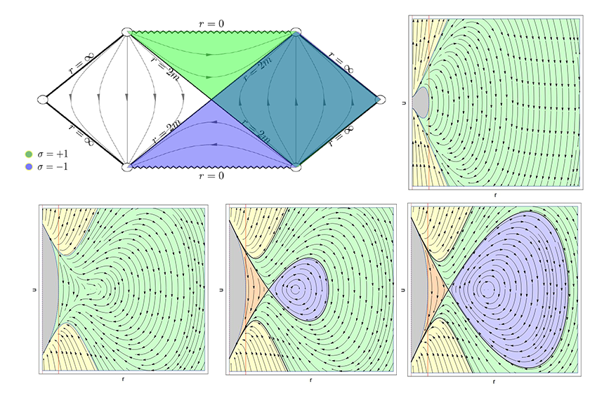
Figure 1: Phase space for timelike particles with increasing value of $L$ from left to right and top to bottom. The dark zone correspond to the forbidden region given by $\epsilon<\frac{\mu}{2}$ and the red line corresponds to the horizon. Different colors are used to distinguish different behaviours for the flow. The upper left image is the Penrose diagram for the Kruskal spacetime where the Kerr-Schild patches have been highlighted.

Let us analyze briefly the Schwarzschild dynamical system. The function $h(r)$ takes the form $h(r)=\frac{2M}{r}$. From Theorems 1 and 4 with the optimal value of $\beta=-\frac{3}{2}$ we derive the geodesic equations

$$r^{\prime} =ru,$$ (7)

$$u^{\prime} =r\left(L^{2}-\mu Mr\right)-3L^{2}M+\frac{3}{2}u^{2},$$ (8)

$$\theta^{\prime} =L\sqrt{r}.$$ (9)

3.1 The collision manifold

The submanifold $r=0$ is clearly invariant under the flow. Since $r=0$ corresponds to the spacetime singularity, this submanifold is called collision manifold. It can be described globally by the coordinates $\{u,\theta\}$ so its topology is $\mathbb{R}\times\mathbb{S}^{1}$. The dynamical system (7)-(9) restricted to the collision manifold reads

$$u^{\prime} =\frac{3}{2}u^{2}-3L^{2}M,$$

$$\theta^{\prime} =0.$$

This system has two lines of critical points: one line of stable points at $(\theta,u)=(\theta_{0},-\sqrt{2ML^{2}})$ and one line of unstable nodes at $(\theta,u)=(\theta_{0},\sqrt{2ML^{2}})$, where $\theta_{0}\in\mathbb{S}^{1}$ is an arbitrary value. For each value of $\theta_{0}$, there is a trajectory extending from $u=-\infty$ and approaching $u=-\sqrt{2ML^{2}}$ as its future limit point, a trajectory from $u=-\sqrt{2ML^{2}}$ to $u=\sqrt{2ML^{2}}$ and a trajectory having $u=\sqrt{2ML^{2}}$ as its past limit point and extending to $u=+\infty$, all of them with $\theta=\theta_{0}$.

3.2 The general flow

We are going to center our attention in the phase portrait for timelike geodesics ($\mu=1$), as this shows more interesting phenomena than in the null case. The fixed points are

$$(r=0,u=\pm\sqrt{2ML^{2}}),\quad\quad(r=r_{\pm}(M,|L|):=\frac{L^{2}\pm|L|\sqrt{L^{2}-12M^{2}}}{2M},u=0),$$

the second pair under the additional condition $L^{2}\geq 12M^{2}$. For $L^{2}>12M^{2}$ all fixed points are hyperbolic, with $(r=r_{+}(M,|L|),u=0)$ being a center (purely imaginary eigenvalues) and $(r=r_{-}(M,|L|),u=0)$ being a saddle. When $L^{2}=12M^{2}$, there is a bifurcation in the phase space, which can be visualized in the transition between the second and third plots in Fig. 1. We thus recover easily all well-known results for geodesics in Schwarzschild outside the horizon. The approach here, however, is perfectly regular both across the horizon at $r=2M$ and even at the singularity $r=0$. Moreover, it allows us to treat all points in the Kruskal spacetime with a single dynamical system.

4 The Reissner-Nordström dynamical system

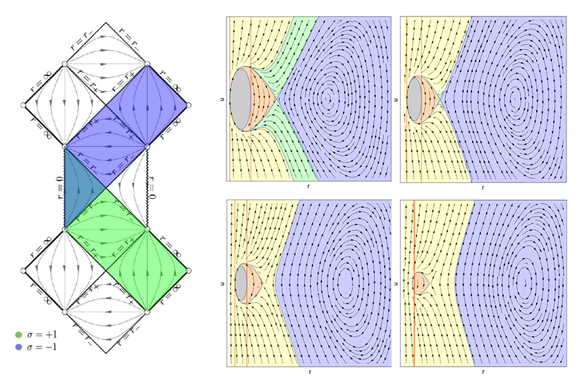
Figure 2: Phase space for timelike particles with fixed value of $L$ increasing value of $Q$ from left to right and top to bottom. The dark zone correspond to the forbidden region and the red line corresponds to the horizons. Different colors are used to distinguish different behaviours for the flow. The left image is the Penrose diagram for the Kruskal spacetime where the Kerr-Schild patches have been highlighted.

Next, we to analyze the Reissner-Nordström dynamical system. The function $h(r)$ is now $h(r)=\frac{2Mr+Q^{2}}{r^{2}}$. From Theorems 1 and 4 with the optimal value of $\beta=-2<\beta_{\text{Schwarzschild}}$ we derive the geodesic equations

$$r^{\prime} =ru,$$ (10)

$$\theta^{\prime} =L\,r,$$ (11)

$$u^{\prime} =r\left(r\left(L^{2}-\mu Mr+\mu Q^{2}\right)-3L^{2}M\right)+2\left(L^{2}Q^{2}+u^{2}\right).$$ (12)

Unlike the Schwarzschild collision manifold, the Reissner-Nordström collision manifold is not reachable by timelike geodesics, which reflects the fact that the singularity for charged black holes is repulsive. More details on the approach of causal geodesics to the collision manifold can be found in [2]. Concerning the general flow for timelike geodesics, the phase diagram has now three critical points and the excluded region shows an interesting behaviour: for $0<|Q|<M$ it detaches from the line $r=0$ and moves across the phase diagram, diminishing for larger values of $Q$ and vanishing when $|Q|=M$. As geodesics can now encircle the excluded region, the variation ranges of Lemma 2 implies (see [2] for details) that any geodesic travelling from $r=r_{0}>r_{+}\to r_{+}\to r_{-}\to r_{1}$ and back to $r_{-}\to r_{+}$ must have changed the Kerr-Schild patch along the way (by changing the value of $\sigma$).

It is interesting to note that inserting $Q=0$ in system (10)-(12) the Schwarzschild case is not recovered. This is because the value of the parameter $\beta$ adapted to Reissner-Nordström is different to that of Schwarzschild. Thus, in the Schwarzschild subcase of Reissner-Nordström we have overkilled the singularity and the fixed points that previously existed at $r=0$, $u=u_{\pm}$ have both collapsed to $u=0$. This collapse can be detected directly on the Reissner-Nordström phase space because the fixed point $\{u=0,\theta=\theta_{0}\}$ is no longer hyperbolic when $Q=0$.

5 References

References

- [1] Belbruno, E., and Pretorius, F. A dynamical system’s approach to Schwarzschild null geodesics. Classical and Quantum Gravity 28, 19 (2011), 195007.
- [2] Galindo, P., and Mars, M. Mcgehee regularization of general so (3)-invariant potentials and applications to stationary and spherically symmetric spacetimes. arXiv preprint arXiv:1405.7627 (2014).
- [3] Kerr, R. P., and Schild, A. A new class of vacuum solutions of the Einstein field equations. Atti del Congregno Sulla Relativita Generale: Galileo Centenario (1965).
- [4] McGehee, R. Double collisions for a classical particle system with nongravitational interactions. Commentarii Mathematici Helvetici 56, 1 (1981), 524–557.