Sampling eigenmodes in colloidal solids

Abstract

We study the properties of correlation matrices widely used in the characterisation of vibrational modes in colloidal materials. We show that the eigenvectors in the middle of the spectrum are strongly mixed, but that at both the top and the bottom of the spectrum it is possible to extract a good approximation to the true eigenmodes of an elastic system.

1092015 10.1209/0295-5075/109/48005

The excitation spectrum of crystalline but also disordered colloidal solids has recently been studied in both two [1, 2, 3, 4] and three [5, 6] dimensions: Experiments typically image a thousand or so micron-sized particles; from a video recording, computer analysis is used to extract a matrix of correlated fluctuations. The hope is that the spectrum and the eigenvectors of the correlation matrix can be used to deduce interesting properties of the colloidal material [7, 8, 9], including local modes and incipient soft structures, or even three dimensional elastic properties [10]. Most experimentalists work with the matrix

$$C_{ij}=\langle\delta r_{i}\delta r_{j}\rangle=\frac{1}{T}\sum_{t=1}^{T}\delta r_{i}(t)\delta r_{j}(t)$$ (1)

where $\delta r_{i}(t)$ denotes a transversion fluctuation (in $x$ and $y$ when imaging along $z$) of a particle at time $t$. For a system of $N$ particles this matrix has dimensions $2N\times 2N$. If the particles are coupled with linear springs the correlation matrix can be related to the interactions as follows

$$C=\frac{1}{\beta A}$$ (2)

where $A$ is the dynamical matrix of the system – at least in the limit of large $T$. Thus the eigenvectors of $C$ and $A$ should be identical and there should be an inverse relationship between the eigenvalues of the two matrices. Even in hard sphere systems the mode structure approximates this linear Ansatz. $\beta$ is the inverse temperature.

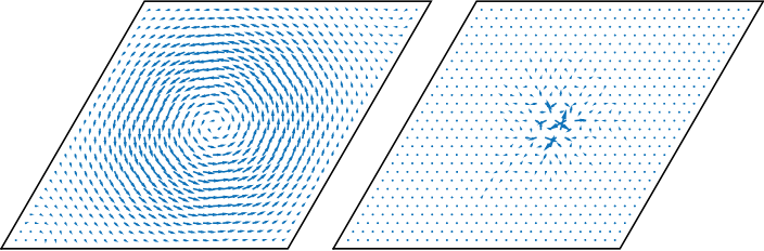
Figure 1: Left: A low-energy mode for an elastic medium eq. (3). Right: High-energy localised mode. Hexagonal lattice with Dirichlet boundary conditions. $N=28^{2}$ particles.

In previous work we considered the question of projection of the modes from three to two dimensions [10, 11]. In this paper we consider the effect of observation statistics on the mode structure. It is already well known [12] that the use of a number of recordings ($T$) which is smaller than the number of observed degrees of freedom ($2N$) leads to a rank-deficient matrix $C$ for which many eigenvalues are zero. Even when $T>2N$ the theory of Marchenko and Pastur [13] shows that there are large systematic (i.e. non-statistical) errors which appear in the spectrum. In fact the observed spectrum is deterministically distorted as a function of $z=T/(2N)$.

The rather remarkable results on the evolution of the spectrum of the correlation matrix are not matched by a detailed theory of the evolution of the eigenvectors; results such as those in ref. [14] tell us about some angular correlations but do not contain the all the information needed by experimentalists to interpret typical data sets. It seems clear that statistical and systematic noise in the sum in eq. (1) will mix eigenmodes, in a manner which is familiar from perturbation theory in quantum mechanics. The point of the present paper is to quantify this mixing in order to give simple rules of thumb as to how many modes can be trusted in a correlation analysis.

Some authors give examples of eigenmodes extracted from the matrix $C$, often coming from different places in the spectrum – for instance low-energy modes, high-energy modes or modes coming deep within the spectrum, such as near a van Hove peak. In the elastic model that we consider a typical low-energy mode is shown in Fig. 1, left. On the right of Fig. 1 we see a high-energy, localised mode of $A$ in a disordered elastic medium. Typically the mode is represented as a series of arrows, with amplitude proportional to the component of the eigenvector at the particle position.

Our main conclusion is that the bottom of the spectrum of $A$, including modes such as that depicted Fig. 1,left is reproduced rather easily on diagonalisation of the correlation matrix. The top of the spectrum depends on the model considered: When we consider the elastic vibrations of a disordered system with strong localisation the top of the spectrum also converges for moderate numbers of samples (though less well than at the bottom). In all cases the middle of the spectrum leads to mixing of an extensive number of eigenvectors, so that little information on the true mode can be observed using a correlation analysis. This is particularly the case near van Hove singularities which seem to strongly favour mode mixing. However, without disorder even the top of the spectrum is badly reproduced; mode reconstruction clearly contains components which are more model dependent than the remarkable Marchenko-Pastur result which depends only on the density of states of the original system.

The experimentalist should also worry about the effect of the finite auto-correlation time for any experimental system. This was studied for the spectrum in a number of papers [15, 16], but no results are available for the effect of correlations on modes. Thus, we conclude with a short study on the influence of finite relaxation rates on the observed mode structure and show that the mode structure is remarkably stable even in the presence of slowly relaxing modes.

1 Elastic model

In this paper we study the modes of a two-dimensional solid, firstly because data in published experiments is recorded from two-dimensional slices but also because two-dimensional elastic systems contain few enough degrees of freedom so that we can use direct matrix solvers to study the mode structure. The study of a three dimensional medium would require more sophisticated iterative algorithms.

We work with a network of central springs with the energy

$$U=\frac{1}{2}\sum_{ij}K_{ij}(r_{ij}-1)^{2},$$ (3)

where $K_{ij}$ is the spring constant between particles $i$ and $j$; $r_{ij}$ is the separation between the particles. We either take the spring constants as equal, in order to study a crystalline material, or we take a model of site disorder where each particle is characterised by a random stiffness $k_{i}$. We set the bond constant $K_{ij}^{-1}=k_{i}^{-1}+k_{j}^{-1}.$ We use a hexagonal lattice which generates an isotropic elastic system obeying the Cauchy relation between the shear and compression modulus [17].

From the energy we generate the matrix

$$A_{ij}=\frac{\partial^{2}U}{\partial r_{i}\partial r_{j}}$$ (4)

of second derivatives as well as the Cholesky factorisation of $A$ which is used to generate the correlation matrix according to the Wishart distribution for $T$ samples [18]. This corresponds to generating the correlation matrix, $C$, as an average of $T$ statistically independent samples. It ignores the possibly slow relaxation of modes in a true experimental sample.

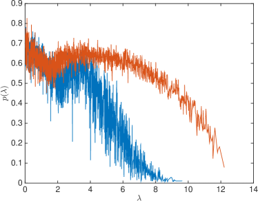
Figure 2: Participation ratios in a elastic medium with disordered elastic constants: from the dynamical matrix $A$ (lower curve, blue), and from the diagonalised correlation matrix $C^{-1}$ (upper curve, red). We see that the system is characterised by a number of high-energy, localised states. The sampled system reproduces this fact rather badly except at very top of the spectrum. $N=28^{2}$, $z=10$. Abscissa $\lambda$ for $A$ and $C^{-1}$. Note the different upper limits in the spectrum due to the Marchenko-Pastur law.

We generate a disordered medium with a strength of disorder which is tuned so that the nature of the modes is qualitatively similar to that observed in experimental systems [4]. In particular we consider in Fig. 2 the participation ratio,

$$\frac{1}{p(\lambda)}=N\sum_{i}v_{i\lambda}^{4}$$ (5)

where $v_{i\lambda}$ is the $i$’th component of the normalized eigenvector with energy $\lambda$. In Fig. 2 we plot $p(\lambda)$ as a function of $\lambda$. $p$ measures, approximately, the proportion of sites over which a mode is localised. For extended modes $p$ is $\mathcal{O}(1)$. For a mode which excites a single site, $p$ is $\mathcal{O}(1/N)$. For an ordered system all modes are extended, however on adding disorder we see that high-energy eigenmodes localize to just a few sites, Fig. 1, right. For the sampling $z=10$ used in Fig. 2 many modes of the matrix $C$ are qualitatively different from those contained in $A$ for large $\lambda$. In particular the modes are often too extended.

2 Characterizing the modes

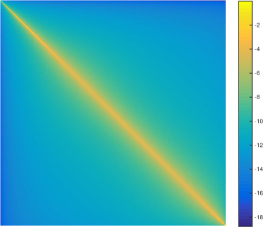
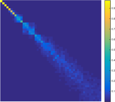
Figure 3: Visualisation of $W$ on a logarithmic scale in order to see the large number of elements with small amplitude. The matrix is strongly diagonally dominant giving a bright central band. Disordered elastic medium, $N=28^{2}$, $z=60$ averaged over $20$ realisations of the disordered matrix $A$. The diagonal dominance implies that it is above all modes with energies which are close in $A$ which are confused in the matrix $C$.

Figure 4: Visualisation of the matrix $W$ (linear scale) zoomed to the lowest energy states of $A$. $N=28^{2}$. Here $C$ is recorded with very poor statistics so that $z=0.75$. Despite this we see that several low-energy states of $A$ are well reproduced in the matrix $C$. Beyond the 7’th mode the amplitude is spread between several modes, which are however still close to the diagonal.

The main tool that we will use to characterise the similitude of modes sampled experimentally and deduced from the original elastic system is the set of overlaps

$$W_{ij}=(u_{i}\cdot v_{j})^{2}$$ (6)

Where $v_{j}$ is the $j$’th eigenvector of $A$ and $u_{i}$ is an eigenvector of $C$, which form a matrix with indices describing the modes of $C$ and $A$. We always sort the modes by increasing eigenvalues for $A$, and by decreasing eigenvalues for $C$. In the case of perfect statistics the matrix $W$ converges to the identity. We also note that each row and column of $W$ sums to unity. We use deviations of $W$ from the identity to quantify non-convergence of the experimental eigenmodes to their final limit. In Fig. 4 we plot $W$ on a logarithmic scale using a colour code to express the amplitude of each element. We are firstly struck by the diagonal domination of the matrix. The bright stripe indicates that modes mostly mix with other modes with similar energies – even if there is also a broad and diffuse background. We also notice that the band is narrower in the top-left and bottom-right corners which correspond to the bottom and the top of the spectrum of $A$. $W$ is more strongly diagonal for these modes and thus the eigenvectors of $C$ are close to eigenvectors of $A$.

We confirm this point by plotting on a linear scale the top left corner of the matrix $W$ corresponding to the lowest-energy states of $A$. In Fig. 4 the strong diagonal for the first modes confirms that the lowest modes in the system are very well reproduced in the correlation matrix. It is only on going higher in the spectrum that we see the broadening which indicates that each eigenvector of $C$ is described by several eigenmodes of $A$. We find that when studying systems with $\mathcal{O}(1000)$ particles even when the system is sampled with $z=0.75$ the very first mode is rather well represented in $C$, even though $C$ is a highly defective matrix.

Figure 5: A cut through the matrix $W$, corresponding to the central row of the matrix $C$. A strong central peak is superposed upon a broader background, $N=48^{2}$, $z=60$. Note that the largest element of $W$ in this slice has an amplitude close to $10^{-2}$ so that hundreds of modes from $A$ are needed to describe the bulk modes of $C$. Vertical lines denote the 90% band width $b$.

3 How does mode mixing scale with $N$ and $z$?

We now examine a row in the middle of the matrix $W$, and plot the amplitude in a log-linear scale in Fig. 5. We see a sharp central peak, superposed on a broader background. We tried to characterise the width of the central peak by using moments of the distribution, however the result was unsatisfactory due to the background in the figure. We chose an alternative method of characterising the signal which was to take the band-width, $b$, which contains 90% of the amplitude. This measure is much more robust to a broad outlying signal and is used to characterise the spreading of modes for the rest of this paper.

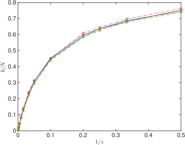
Figure 6: 90% bandwidth, $b$ of $W$ for several different systems sizes, measured for $z=60$, $N=38^{2}$, $N=18^{2}$, $N=38^{2}$, $N=58^{2}$. Plotted from top left to bottom right of the matrix. The band width increases quadratically near the top left of the matrix, corresponding to the lowest-energy modes of $A$. In the centre of the matrix there is a broad range of modes where an extensive fraction of eigenmodes are mixed together. For the highest-energy modes of $A$ the matrix $C$ again gives a good representation of the mode structure for a very small number of modes. Disordered system.

Figure 7: 90% bandwidth of the middle mode of $W$ as a function of the inverse sampling, $1/{z}$. Data for different system sizes fall onto a single master curve. $N=18^{2}$, $N=28^{2}$, $N=38^{2}$, $N=58^{2}$. Disordered system.

In Fig. 7 we choose several different sample sizes and plot the 90% width, $b$ scaled by the number of particles as a function of the rank of the mode in the spectrum, $n$. Each correlation matrix was recorded with $z=60$ corresponding to a high-statistics experiment. We see that all system sizes behave in a similar manner. For both high and low energies the band-width of the matrix is small, but for most interior modes in $C$ the band width is $\mathcal{O}(0.16N)$. Thus a single mode in $C$ is actually a mixture of an extensive number of modes in $A$. In Fig. 7 we consider a single system size and plot $b$ as a function of $1/{z}$. The curve comes to the origin linearly: It seems clear that extracting accurate eigenmodes in the middle of the spectrum is a very difficult task requiring very large values of $z$ if the only information available is the correlation matrix $C$.

We also performed a similar study on the matrix $C$ for an ordered elastic medium in which all the spring constants are identical. The conclusions for the low-lying and middle modes of $A$ are very similar. However curves such as Fig. 7 are rather different for the highest-energy modes. There is a weaker drop of the curve on the right towards zero and the top-most modes are badly represented by the eigenmodes of $C$. Thus there seem to be some non-universal features in the manner that eigenmodes of $C$ are represented in the modes of $A$; only the lowest modes are faithfully represented in all systems. The representation of the topmost modes is clearly model dependent.

We plot in Fig. 8 the full bandwidth curves for a crystal for $N=58^{2}$ for several different values of $z$; In this curve different parts of the spectrum behave in different ways. For low energies and for $n/2N\sim 0.5$ there is a convergence of the scaled curves for large $z$. This is the same convergence behaviour that we saw in Fig. 7. Very differently, for positions in the spectrum which seem to be associated with the van Hove singularities there is a continuous evolution of the spectrum with $z$. This continuous evolution is not seen for disordered systems for which the whole curve seems to stabilise for large $z$ (data not shown).

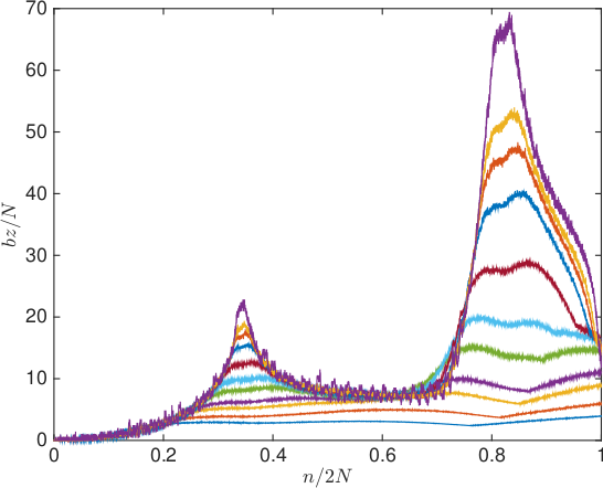
Figure 8: The 90% bandwidth is plotted for the matrix $W$ for a perfect crystal. $N=58^{2}$, for different $z$ varying from $z=1$ (flattest curves) to $z=3200$ (strongest peaks). We see that large numbers of modes are well reproduced for small $n$ but far fewer modes are well reproduced at the top of the spectrum. The peaks are associated with the appearance of van Hove peaks in the density of states which seem to favour mode mixing, and a broader band in $W$.

4 How many modes are reliable?

We finish with a study of how many modes in $C$ are reliable. At both the bottom and the top of the spectrum of $A$ we find how many modes are reproduced within $C$ with a matrix element $W_{ij}>0.5$. We plot the results independently for the top and bottom of the spectrum in Fig. 9. The most remarkable result is a rather good empirical scaling so that the number of well reproduced modes $m$ at the bottom of the spectrum

$$m\approx\sqrt{Nz}/3\sim\sqrt{T}\quad\text{ independent of N}$$ (7)

This law works over large variations of $z$, $N$ and depends weakly on the degree of disorder in the elastic medium.

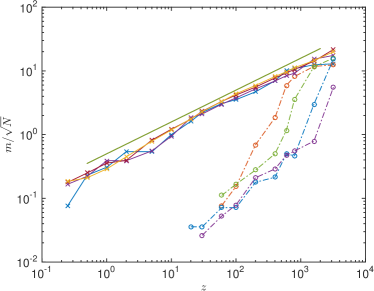
Figure 9: Number of good modes as a function of $z$. $N=18^{2}$, $N=28^{2}$, $N=38^{2}$, $N=58^{2}$. Straight line as a guide to the eye, $m=\sqrt{zN}/2$. Data from bottom of spectrum of $A$, collapse to a single master curve. Data from top of the spectrum do not collapse with this scaling. We only start seeing well resolved modes at the top of the spectrum for $z>20$. Numbers resolved at the top and bottom of the spectrum only become comparable for $z\sim 1000$. Disordered system.

The data coming from the top of the spectrum is much noisier and does not exhibit a clean scaling with $N$ or $z$. Indeed we also find qualitatively different results between ordered and disordered systems – in an ordered system no modes are resolved at the top of the spectrum. The resolution that we find in the disordered system is perhaps linked to the localised nature of the modes.

5 Effects of sampling rate

We now consider the effects of finite relaxation times in an experimental system. We know that long-wavelength modes relax more slowly than those describing the shortest length scales. Since it is these modes which are best described in the spectrum of $C$ we might fear a degradation of the method due to rapid sampling. A full account would require a two fluid theory of colloidal dynamics [19], we here use a simpler description with a Langevin equation which gives a qualitatively correct description of the slowest, over-damped, longitudinal modes. Thus we study a set of $2N$ coordinates evolving according to the equation

$$\frac{dr}{dt}=-Ar+\xi(t)$$ (8)

where $r$ is a vector and $\xi$ is a vector of Brownian noise, $\langle\xi_{i}(t)\xi_{j}(s)\rangle=\delta_{ij}\delta(t{-}s)\,2/\beta$.

We sample the positions regularly with a time step $\tau$ which is a fraction $f$ of the relaxation rate of the slowest mode of the Langevin equation.

$$\tau=f/\lambda_{1}$$ (9)

with $\lambda_{1}$ the smallest eigenvalue of $A$. This gives the following update rule for the positions:

$$r^{\prime}=e^{-\tau A}r+\sum_{i}{\mathcal{N}}(0,\sigma_{i})v_{i}$$ (10)

with ${\mathcal{N}}(0,\sigma)$ normally distributed random numbers with mean zero and variance $\sigma^{2}$. They are independent for different $i$. As above, $v_{i}$ is the eigenvector corresponding to $\lambda_{i}$. For the equation (8) we find the variance for each mode,

$$\sigma_{i}^{2}=\frac{1}{\beta\lambda_{i}}\left[1-e^{-2\tau\lambda_{i}}\right].$$ (11)

We then build up our estimate of the covariance matrix using eq. (1) with $T=2Nz$ samples. When $\tau$ is large each mode is sampled independently as in the Wishart ensemble considered above. When $\tau$ is very small the positions remain highly correlated between successive samples.

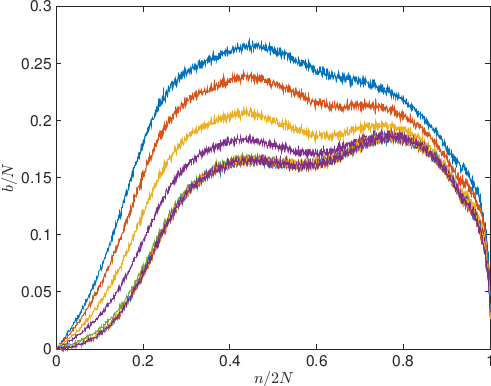
Figure 10: Effect of autocorrelation on the mode resolution: eq. (9) $f=[.004\,.005\,.007\,.01\,.02\,.04\,.06\,.1\,.5\,1\,2.]$ from highest to lowest curve, $N=28^{2}$, $z=40$. Already curves with $f=.02$ are well converged. All curves for high values of $f$ superpose.

We plot the bandwidth analysis of the dynamics, eq. (10), in Fig. 10. We find the results most surprising: Already for the small value $f=0.02$ the resolution of modes within $C$ is very close to that found in our above study of the Wishart ensemble. Even though the modes are sampled very inefficiently, the diagonalisation is able to resolve the lowest modes within the system. Indeed in the given example with $z=40$ and $f=0.02$ the system is simulated for not quite one relaxation time of the slowest mode; despite this the global appearance of the bandwidth is close to the fully converged ensemble with the same value of $z$.

6 Conclusion

We have carried out a numerical study of the mode structure of correlation matrices, of the sort commonly extracted from colloidal materials. The lowest eigenvectors of $A$, (which correspond to the top eigenvectors of $C$) are rather easily extracted from the matrix. However within the bulk of the spectrum there is a mixing of an extensive proportion of the exact modes for values of $z$ typically used in experiments. In the case of disordered materials it is possible to study just a few eigenvectors at the top of the spectrum of $A$, even though the top eigenvalues converge rather badly in the Marchenko-Pastur theory. One of the most surprising features of our results is the convergence of high-energy modes in the spectrum, which has not been observed in earlier work [12]. However the authors of this study worked very close to the limit $z=1$ where the convergence of these highest modes is not yet visible. Such large-z studies have now been published by several experimental groups.

When we added the effect of finite relaxation times in the construction of the correlation matrix we discovered that the lowest modes are resolved with remarkably low statistics.

References

- [1] \NameZahn K., Wille A., Maret G., Sengupta S. Nielaba P. \REVIEWPhys. Rev. Lett.902003155506.
-
[2]
\NameKeim P., Maret G., Herz U. von Grünberg H. H. \REVIEWPhys. Rev.
Lett.922004215504.
http://prl.aps.org/abstract/PRL/v92/i21/e215504 - [3] \NameChen K., Ellenbroek W. G., Zhang Z., Chen D. T. N., Yunker P. J., Henkes S., Brito C., Dauchot O., van Saarloos W., Liu A. J. Yodh A. G. \REVIEWPhys. Rev. Lett.1052010025501.
-
[4]
\NameChen K., Still T., Schoenholz S., Aptowicz K. B., Schindler M., Maggs
A. C., Liu A. J. Yodh A. G. \REVIEWPhys. Rev. E882013022315.
http://link.aps.org/doi/10.1103/PhysRevE.88.022315 -
[5]
\NameGhosh A., Mari R., Chikkadi V., Schall P., Maggs A. Bonn D.
\REVIEWPhysica A: Statistical Mechanics and its
Applications39020113061 .
http://www.sciencedirect.com/science/article/pii/S037843711100207X - [6] \NameGhosh A., Chikkadi V. K., Schall P., Kurchan J. Bonn D. \REVIEWPhys. Rev. Lett.1042010248305.
-
[7]
\NameWyart M., Nagel S. R. Witten T. A. \REVIEWEPL (Europhysics
Letters)722005486.
http://stacks.iop.org/0295-5075/72/i=3/a=486 -
[8]
\NameDuring G., Lerner E. Wyart M. \REVIEWSoft Matter92013146.
http://dx.doi.org/10.1039/C2SM25878A -
[9]
\NameBrito C. Wyart M. \REVIEWJournal of Statistical Mechanics: Theory
and Experiment20072007L08003.
http://stacks.iop.org/1742-5468/2007/i=08/a=L08003 -
[10]
\NameLemarchand C. A., Maggs A. C. Schindler M. \REVIEWEPL (Europhysics
Letters)97201248007.
http://stacks.iop.org/0295-5075/97/i=4/a=48007 -
[11]
\NameSchindler M. Maggs A. C. \REVIEWSoft Matter820123864.
http://dx.doi.org/10.1039/C2SM07117G -
[12]
\NameHenkes S., Brito C. Dauchot O. \REVIEWSoft Matter820126092.
http://dx.doi.org/10.1039/C2SM07445A - [13] \NameMarchenko V. Pastur L. \REVIEWMath. USSR, Sb.11968457.
-
[14]
\NameAllez R. Bouchaud J.-P. \REVIEWPhys. Rev. E862012046202.
http://link.aps.org/doi/10.1103/PhysRevE.86.046202 -
[15]
\NameSengupta A. M. Mitra P. P. \REVIEWPhys. Rev. E6019993389.
http://link.aps.org/doi/10.1103/PhysRevE.60.3389 -
[16]
\NameBurda Z., Görlich A., Jurkiewicz J. Wac¿aw B. \REVIEWThe
European Physical Journal B - Condensed Matter and Complex
Systems492006319.
http://EconPapers.repec.org/RePEc:spr:eurphb:v:49:y:2006:i:3:p:319-323 - [17] \NameBorn M. Huang K. \BookDynamical Theory of Crystal Lattices (Oxford University Press, Oxford) 1998.
-
[18]
\NameSmith W. B. Hocking R. R. \REVIEWJ. Appl. Stat211972341.
http://lib.stat.cmu.edu/apstat/53 -
[19]
\NameHurd A. J., Clark N. A., Mockler R. C. O’Sullivan W. J.
\REVIEWPhys. Rev. A2619822869.
http://link.aps.org/doi/10.1103/PhysRevA.26.2869