Fidelity and Reversibility in
the Restricted Three Body Problem

Abstract

We use the Reversibility Error Method and the Fidelity to analyze the global effects of a small perturbation in a non-integrable system. Both methods have already been proposed and used in the literature but the aim of this paper is to compare them in a physically significant example adding some considerations on the equivalence, observed in this case, between round-off and random perturbations.

As a paradigmatic example we adopt the restricted planar circular three body problem. The cumulative effect of random perturbations or round-off leads to a divergence of the perturbed orbit from the reference one. Rather than computing the distance of the perturbed orbit from the reference one, after a given number $n$ of iterations, a procedure we name the Forward Error Method (FEM), we measure the distance of the reversed orbit ($n$ periods forward and backward) from the initial point. This approach, that we name Reversibility Error Method (REM), does not require the computation of the unperturbed map. The loss of memory of the perturbed map is quantified by the Fidelity decay rate whose computation requires a statistical average over an invariant region. Two distinct definitions of Fidelity are given. The asymptotic equivalence of REM and FEM is analytically proved for linear symplectic maps with random perturbations. For a given map, the REM plot provides a picture of the dynamic stability regions in the phase space, very easy to obtain for any kind of perturbation and very simple to implement numerically. The REM and FEM for linear symplectic maps are proved to be asymptotically equivalent. The global error growth follows a power law in the regions of integrable (or quasi integrable) motion and an exponential law in the regions of chaotic motion. We prove that the power law exponent is $3/2$ for a generic anisochronous system, but drops down to $1/2$ if the system is isochronous. Correspondingly the Fidelity $F(t)$ exhibits an exponential decay and $-\ln F(t)$ grows just as the square of the FEM or REM error. The Reversibility Error and Fidelity can be used for a quantitative analysis of dynamical systems and are suited to investigate the transition regions from chaotic to regular motion even for Hamiltonian systems with many degrees of freedom such as the $N$-body problem.

1 Introduction

The dynamics of non-integrable Hamiltonian systems is qualitatively well understood when it reduces to an area preserving map on the Poincaré section. This is the case of the $3$-body problem. However the orbits, for generic initial conditions, can only be obtained by numerical integration [1, 2]. The symplectic integration schemes preserve the Poincaré invariants [3, 4] but are affected by local discretization errors and round-off ([5, 6] and reference therein for a recent review on the topic). Therefore, it is important to be able to estimate the divergence of the numerically integrated orbit with respect to the exact one. With a sufficiently small integration step the local integration error can be lowered down close to the round-off level. For a recent and comprehensive presentation of geometric integration methods, their accuracy and stability see [7]. By slightly changing the initial point in phase space we explore the sensitivity of the map to initial conditions. The Lyapunov Error Method (LEM) is based on the distance of the reference orbit from another orbit with a close initial condition. The definition is given at the beginning of Section 3. The asymptotic analysis provides the Lyapunov spectrum. The rigorous analysis developed by [8, 9] has a numerical counterpart [10], and several methods to explore the asymptotic behavior of LEM have been proposed [11]. The dynamic stability of the map, namely its sensitivity to small random perturbations or to round-off, is another relevant issue. The Forward Error Method (FEM) consists in evaluating the divergence of the perturbed orbit from the reference orbit. We do not consider deterministic perturbations since an extended literature exists at least when the map is integrable or uniformly hyperbolic [12]. To analyze the round-off effects a convenient approach is based on the Reversibility Error Method (REM), which consists in computing the divergence of the initial point from its image after $n$ forward and $n$ backward iterations of the perturbed map, avoiding the exact computation of the map. This method is usually known as Reversibility test [13] and it is routinely used to analyze the regularization method for close encounters between two massive objects [14], or in the electromagnetic problems [15], or to study the collisions in the few body gravitational problem [16]. It has also been used to investigate the dynamic stability of the Hamiltonian model $H=p^{2}/2-1/x+\epsilon x\cos(\omega t)$ [17]. We might expect that, asymptotically, REM and FEM have a similar behavior. If the error is random we rigorously prove the equivalence of REM and FEM asymptotic behavior in the case of linear symplectic maps. To our knowledge this is a new result and can be extended to the non linear case. The extension of the proof to non linear maps requires more sophisticated mathematical tools such as in [8], and is not afforded here, even though we carry out the basic preliminary steps. Our numerical simulations suggest that this equivalence holds also for non linear maps. For chaotic orbits, which have a positive maximum Lyapunov characteristic exponent $\lambda>0$, the asymptotic divergence of REM, FEM and LEM is governed by the same exponential law. For regular orbits, which have $\lambda=0$, the asymptotic divergence follows a power law, with exponent $\beta$. If the perturbation is random the exponent for REM and FEM is $\beta=3/2$ for a generic observable (for instance the separation) and for a generic anisochronous system. If the system is isochronous the exponent reduces to $\beta=1/2$. If the observable is a first integral the exponent is also $\beta=1/2$. The Lyapounov error growth follows a power law with exponent $1$ for a generic observable and for a generic anisochronous system. For and isochronous system or if the observable is a first integral the exponent is $\beta=0$. We provide a rigorous justification to the above statements on the power law exponents for LEM, FEM and LEM and a numerical check for the restricted planar circular $3$-body problem. In the case of round-off the same power laws for REM are observed, provided that the map, in the chosen coordinates system, is sufficiently complex from the computational viewpoint. As a counterpart of FEM we propose the Fidelity [18], which measures the correlation between the unperturbed and perturbed orbits. The Fidelity decay law is related to the asymptotic growth of the global error. A correspondence with REM is achieved by defining the Fidelity as the correlation between an observable computed on the initial point and its image after $n$ forward and $n$ backward iterations of the perturbed map. Rigorous results on the Fidelity for prototype dynamical models with random perturbations are already known [19]. The comparison of REM for round-off and noise was considered in [20] and extended to the Fidelity in [21, 22]. In the present paper we show that for the planar circular three body problem REM, FEM and Fidelity are suitable to investigate the effects of small random perturbations, whereas REM and the corresponding Fidelity are suitable to explore the round-off effects. The $3$-body problem is the paradigm of systems in which both regular and chaotic orbits coexist in a very narrow region of the phase space and can provide a significant insight in astrophysical relevant problems (see reference [23], for a detailed discussion about the $3$-body problem and its application in astrophysics). The results previously obtained on prototype dynamical models are confirmed and extended. Even though in the neighborhood of the equilibria or periodic points in the rotating system the Birkhoff normal forms can be used to approximate the quasi-integrable dynamics with an integrable one (obtaining Nekhoroshev stability estimates from bounds on the remainder), the numerical integration procedure cannot be avoided to explore the whole phase space in the Poincaré section. The computation of REM on a grid of points in phase space for a fixed number $n$ of iterations and its visualization provides an easy insight on the dynamic stability of a map. Its use may be convenient to explore the boundary between regions of regular and chaotic motion. The Fidelity allows to quantify the perturbation size and to determine the memory loss rate of the orbits in a given invariant domain. It provides information of statistical nature but it is also computationally more demanding since a Monte-Carlo sampling of the invariant domain is required. The REM and Fidelity are particularly suited to explore the transition regions in complex dynamical systems with many degree of freedom. The paper has 6 sections. Section 1: introduction. Section 2: the $3$-body Hamiltonian in the fixed frame, in the rotating frame and their symplectic integrators. Section 3: analytic proof of the asymptotic equivalence of REM and FEM, for a linear symplectic map with a stochastic perturbation. Section 4: numerical analysis of REM for round-off, of REM and FEM for random perturbations and comparison with LEM. Section 5: definition of Fidelity and numerical results. Section 6: conclusions.

2 Three body Hamiltonian

The restricted planar circular three body problem (see for instance [24] for a detailed description of this problem) consists in a primary central body of mass $m_{1}$, a secondary body of mass $m_{2}\leq m_{1}$ describing circular orbits around their center of mass, and a third body of mass $m_{3}$, so small that it does not perturb the motion of the first two bodies. We consider two reference frames: the fixed inertial frame with the origin on the center of mass and the rotating frame with the same origin and where the first two bodies are at rest. As customary we scale the space coordinates with the distance $r_{*}$ between the massive bodies and the time with $2\pi/T_{*}$ where $T_{*}$ is the period of the circular motion (see [25] for details). Denoting with $t$ the scaled time and $x_{F},y_{F}$ the scaled coordinates of the third body in the fixed frame, the Hamiltonian in the extended phase space, where we introduce a new coordinate $\tau$ and its conjugate momentum $p_{\tau}$, reads

$$H_{F}=T_{F}+V_{F},\qquad\qquad T_{F}={p_{x\,F}^{2}+p_{y\,F}^{2}\over 2}+p_{\tau},\qquad\qquad V_{F}=-{1-\mu\over r_{1}}-{\mu\over r_{2}},\qquad\mu=\frac{m_{2}}{m_{1}+m_{2}}$$ (1)

The potential is a periodic function of $\tau$ with period $2\pi$ and $H_{F}$ is a first integral of motion. Notice that $\tau$ is an angle, its conjugate momentum $p_{\tau}$ is an action and that $t=\tau$. In the rotating frame the first and second bodies are on the $x$ axis with coordinates $x_{1c}=-\mu$ and $x_{2c}=1-\mu$ and the distances $r_{1},r_{2}$ of the third body from the first two in the fixed frame are given by

$$r_{1}=\sqrt{(x_{F}+\mu\cos\tau)^{2}+(y_{F}+\mu\sin\tau)^{2}}\quad r_{2}=\sqrt{(x_{F}-(1-\mu)\,\cos\tau)^{2}+(y_{F}-(1-\mu)\,\sin\tau)^{2}}$$ (2)

assuming the rotation of the massive bodies with respect to the fixed frame is counter-clockwise. The one period map is just the Poicaré section $\tau=0\,\hbox{mod}\,2\pi$ in the fixed frame. In the rotating frame the coordinates of the third body are $x,y$ and the Hamiltonian is given by

$$H=T+V\qquad\qquad T={p_{x}^{2}+p_{y}^{2}\over 2}+yp_{x}-xp_{y}\qquad\qquad V=-{1-\mu\over r_{1}}-{\mu\over r_{2}}$$ (3)

where the distances are now expressed by

$$r_{1}=\sqrt{(x+\mu)^{2}+y^{2}},\qquad\qquad r_{2}=\sqrt{(x-1+\mu)^{2}+y^{2}}$$ (4)

The Hamiltonian is conserved $H=-J/2=E$ where $E$ is the energy and $J$ the Jacobi integral. The first integral $H$ can be written as the sum of the kinetic energy plus the effective potential, sum of the gravitational and the centrifugal potentials

$$H={{\dot{x}}^{2}+{\dot{y}}^{2}\over 2}+V_{\rmsmm\hbox{ {eff} }}(x,y)\qquad\qquad V_{\rmsmm\hbox{ {eff} }}=V-\frac{x^{2}+y^{2}}{2}$$ (5)

The coordinates of the Lagrange equilibrium points $L_{4}$ and $L_{5}$ (critical points of $V_{\rmsmm\hbox{ {eff} }}$) are given by $x_{c}=1/2-\mu,\;y_{c}=\pm\sqrt{3}/2$. The massive bodies and $L_{4}$ or $L_{5}$ are the vertices of an equilateral triangle. We are interested in the evolution of the system in the rotating frame: as a consequence may either integrate the equations of motion of the Hamiltonian 3. As an alternative, we transform the initial conditions to the fixed frame, integrate the equations of motion of the Hamiltonian 1, and transform back to the rotating frame whenever it is needed. The last one is the procedure we adopt. We choose $\mu=0.000954$ which corresponds approximately to the Jupiter-Sun masses and fix the Jacobi constant $J=3.07$ close to the value $J_{c}=-2V_{\rmsmm\hbox{ {eff} }}(x_{c},y_{c})=3-\mu+\mu^{2}$ assumed at the equilibrium points $L_{4},\,\,L_{5}$ [26]. Our numerical analysis is referred to a 3D manifold $\cal{M}_{J}$ in the 4D phase space, specified by a given value of the Jacobi constant $J$. We consider the 2D manifold $\cal{M}_{P}=\cal{M}_{J}\cap\cal{L}$ obtained by intersecting the Jacobi manifold with the linear manifold ${\cal L}:\{y=0$ and $\dot{y}>0\}$. The projection of ${\cal M}_{P}$ into the $(x,\dot{x})$ phase plane is a domain defined by

$${\dot{x}}^{2}\leq x^{2}+2\,{1-\mu\over|x+\mu|}+2\,{\mu\over|x-1+\mu|}-J$$ (6)

The initial conditions are chosen in ${\cal M}_{P}$ and we examine the intersections of the orbit with ${\cal M}_{P}$. Their projections on the $(x,\dot{x})$ or $(x,p_{x})$ phase planes are considered for visualization. For each orbit the initial conditions are $x(0)=x_{0}$, $y(0)=0$ and $\dot{x}(0)=v_{x\,0}$ chosen so that the inequality 6 is satisfied. The remaining initial condition $\dot{y}(0)$ is then given by

$$\dot{y}(0)=\sqrt{x_{0}^{2}-{v_{x\,0}}^{2}+2\,{1-\mu\over|x_{0}+\mu|}+2\,{\mu\over|x_{0}-1+\mu|}-J}$$ (7)

Symplectic integrator maps and errors We consider the fourth order symplectic and symmetric integrator for the evolution, in the fixed and rotating frame, generated by the Hamiltonians 1 and 3. The splitting of the Hamiltonian into two integrable components allows to introduce a second order symplectic and symmetric evolution operator. By three compositions of the second order operator, the fourth order symplectic and symmetric operator is obtained [27]. The Lie derivative for the time independent Hamiltonian $H$ is denoted by $D_{H}$ and the corresponding evolution operator in a time interval $t$ is the Lie series $e^{t\,D_{H}}$. In the fixed frame we split the Hamiltonian $H_{F}$ according to equation 1 and the evolution generated by $T_{F}$ and $V_{F}$ can be exactly computed. The symmetric second order scheme is defined by

$${\char 77\relax}^{(2)}_{{\Delta t}}\equiv e^{\Delta t/2\,\,D_{V_{F}}}\,\,e^{\Delta t\,\,D_{T_{F}}}\,\,e^{\Delta t/2\,\,D_{V_{F}}}$$ (8)

the operator ${\char 77\relax}^{(2)}_{{\Delta t}}$ advances the phase space vector ${\bf x}_{F}=(x_{F},y_{F},\tau,p_{xF},p_{yF},p_{\tau})$ from time $t$ to time $t+\Delta t$ with an error of order $(\Delta t)^{3}$. The fourth order scheme is defined by

$${\char 77\relax}^{(4)}_{{\Delta t}}={\char 77\relax}^{(2)}_{\alpha\Delta t}\,\,{\char 77\relax}^{(2)}_{\beta\Delta t}\,\,{\char 77\relax}^{(2)}_{\alpha\Delta t},\qquad\qquad\alpha={1\over 2-2^{1/3}},\qquad\beta=1-2\alpha<0.$$ (9)

The triple composition of the maps corresponding to the second order evolution generates a symplectic map which advances ${\bf x}_{F}$ from $t$ to $t+\Delta t$ with an error $O(\Delta t)^{5}$. The procedure to obtain the symplectic integrators in the rotating frame is the same. With the splitting of the Hamiltonian according to equation 3 the symmetric second order scheme in this case is given by

$${\char 77\relax}^{(2)}_{\Delta t}=e^{\Delta t/2\,\,D_{V}}\,\,e^{\Delta t\,D_{T}}\,\,e^{\Delta t/2\,\,D_{V}}$$ (10)

the new operator ${\char 77\relax}^{(2)}_{\Delta t}$ advances the phase space vector ${\bf x}=(x,y,p_{x},p_{y})$ from time $t$ to time $t+\Delta t$ with an error of order $(\Delta t)^{3}$. The fourth order scheme is defined by 9 as in the previous case. Higher order schemes are very easily obtained. For instance the sixth order scheme is given by equation 9 where $M^{(4)}$ and $M^{(2)}$ are replaced by $M_{6}$ and $M_{4}$ with $\alpha=1/(2-2^{1/5})$. The eight order scheme is given by equation 9 where $M_{4}$ and $M_{2}$ are replaced by ${\char 77\relax}^{(8)}$ and ${\char 77\relax}^{(6)}$ with $\alpha=1/(2-2^{1/7})$. The number of evaluations of ${\char 77\relax}^{(2)}$ for integrators of order $2m$ grows as $3^{m-1}$ (optimized algorithms lower this number to $7$ for $m=3$ and to $15$ for $m=4$ see [27]). The local error of order $({\Delta t})^{2m+1}$ introduces fluctuations $\Delta H/H$ of order $(\Delta t)^{2m}$ along the orbit. Even though high order integrators seem to be convenient, the appearance of numerical instabilities for large $m$ suggest the choice $m=2$ as a reasonable compromise for our numerical exploration of the effects of round-off and random perturbations. To any evolution operator ${\char 77\relax}$ corresponds a map $M$, to operators multiplication corresponds the composition of maps. To ${\char 77\relax}^{(2)}_{{\Delta t}}$ and its inverse ${{\char 77\relax}^{(2)}_{{\Delta t}}}^{-1}$ we associate the maps $M^{(2)}_{{\Delta t}}$ and ${M^{(2)}_{{\Delta t}}}^{-1}$ and we denote $M^{(2)}_{\epsilon,\,{\Delta t}}$ and ${M^{(2)}_{\epsilon,\,{\Delta t}}}^{-1}$ the corresponding maps with a round-off or random perturbation of amplitude $\epsilon$. The perturbed inverse ${M^{(2)}_{\epsilon,\,{\Delta t}}}^{-1}$ is not the inverse of the perturbed map so that

$$\bigl{(}{M^{(2)}_{\epsilon,\,{\Delta t}}}^{-1}\circ M^{(2)}_{\epsilon,\,{\Delta t}}\bigr{)}({\bf x})\not={\bf x}$$ (11)

The fourth order perturbed map $M^{(4)}_{\epsilon,\,{\Delta t}}$, obtained as the composition of three second order perturbed maps, is also irreversible. The forward error $M^{n}_{\epsilon}({\bf x}_{0})-M^{n}({\bf x}_{0})$ and the reversibility error $M^{-n}_{\epsilon}\circ M^{n}_{\epsilon}({\bf x}_{0})-{\bf x}_{0}$ can be analyzed for different choices of the symplectic map $M$. In the scaled variables the period is $T=2\pi$ and the time step we choose is ${\Delta t}=T/n_{s}$, where $n_{s}$ is an integer. In the next Section we choose $M$ to be the one period map $M=\left({M^{(4)}_{{\Delta t}}}\right)^{n_{s}}$ obtained from the Hamiltonian $H_{F}$ in the fixed frame. As a consequence the local error on the map $M_{\epsilon}$ is the global error of $M^{(4)}_{\epsilon,\,{\Delta t}}$ after $n_{s}$ iterations.
In Section 4 to compute the Fidelity we choose $M$ to be the Poincaré map in the rotating frame, as before the map is computed using the symplectic integrator in the fixed frame. The intersection with the hyperplane $y=0$ can be computed using linear interpolation if the stochastic perturbation of the map is large with respect to the interpolation error ($\sim 10^{-10}$). An interpolation to machine accuracy is provided by the Hénon method [28] but its application is straightforward only if $M^{(4)}_{{\Delta t}}$ is the symplectic integrator in the rotating frame.

3 Asymptotics of Lyapunov, Forward and Reversibility Errors

In this section we analyze the asymptotic behavior of the forward and reversibility errors. Even though we may expect that the behavior is the same a mathematical proof is necessary to make this expectation a solid statement. Assuming the amplitude $\epsilon$ of the local perturbation is infinitesimal, the general expression for the global forward and reversibility errors are obtained at first order in $\epsilon$. Explicit asymptotic expressions are given for random perturbations in the case of linear maps. As a consequence the power law growth of the global error for an integrable map and the exponential growth for an expanding (chaotic) map are easily recovered. Extending the proof to non linear maps requires a more sophisticated mathematical apparatus.

3.1 Lyapunov error

Let us consider a symplectic map $M({\bf x})$ and its orbit ${\bf x}_{n}=M({\bf x}_{n-1})$ with initial point ${\bf x}_{0}$. Consider a nearby point ${\bf x}_{0}+\epsilon\,{\bf e}$, as initial condition for another orbit, where ${\bf e}$ is a vector of norm 1 and $\epsilon$ is a small parameter. The Lyapunov error is defined as the distance of these orbits after $n$ iterations

$$d^{(L)}_{n}=\|M^{n}({\bf x}_{0}+\epsilon\,{\bf e})-M^{n}({\bf x}_{0})\|.$$ (12)

The asymptotic limit of this error, defined by

$$\lambda=\lim_{n\to\infty}\lim_{\epsilon\to 0}\,\ln{\left(d^{(L)}_{n}\over\epsilon\right)},$$ (13)

gives, for almost all the directions ${\bf e}$ (namely for all the points on the unit sphere $\|{\bf e}\|=1$ except for a set of measure zero) the maximum Lyapunov exponent. If the system is ergodic, or if we consider an ergodic component, the limit is the same for almost all initial conditions ${\bf x}_{0}$. If we consider the parallelepiped (parallelotopes) ${\char 80\relax}_{k}$, whose sides are $\epsilon\,{\bf e}_{i}$ for $i=1,2,\ldots,k$ and $k$ ranges from $2$ up to the phase space dimension $d$, supposing ${\bf e}_{i}$ are linearly independent vectors, the asymptotic behavior of the volumes of ${\char 80\relax}_{k}$ determines the Lyapunov spectrum, see [8, 9].

3.2 Forward error

Rather than considering, for a given map, the error due to an initial displacement to analyze the sensitivity to initial conditions, we may consider a small perturbation of the map to explore the sensitivity to small changes of the laws of motion. We denote with $M_{\epsilon}({\bf x})$ the perturbed map, where the perturbation is due to round-off or random errors. As explained in the introduction we do not consider small deterministic perturbations due to abundant literature on the subject. The orbit of the perturbed map is defined by

$${\bf x}_{\epsilon,\,n}=M_{\epsilon}({\bf x}_{\epsilon,\,n-1})=M({\bf x}_{\epsilon,\,n-1})+\epsilon{\mathchar 28952\relax}_{n},\qquad\qquad n\geq 1,$$ (14)

The initial point ${\bf x}_{\epsilon,\,0}={\bf x}_{0}+\epsilon{\mathchar 28952\relax}_{0}$ can be perturbed, but we shall assume it is not, choosing ${\mathchar 28952\relax}_{0}=0$. With $\epsilon$ we denote the perturbation amplitude. For a given round-off error of amplitude $\epsilon$ the exact map $M$ can only be approximated by using a higher accuracy (where the round-off error is typically $\epsilon^{2}$). The round-off error is defined by $\epsilon{\mathchar 28952\relax}_{n}=M_{\epsilon}({\bf x}_{\epsilon,\,n-1})-M({\bf x}_{\epsilon,\,n-1})$. In the case of a random perturbation we may evaluate $M$ with the selected machine accuracy provided that $\epsilon$ is larger by some orders of magnitude with respect to the round-off. The ${\mathchar 28952\relax}_{n}$ are independent random vectors whose components have zero mean and unit variance. The global error at step $n$ is defined by

$$\epsilon{\mathchar 28932\relax}_{n}={\bf x}_{\epsilon,\,n}-{\bf x}_{n}=M^{n}_{\epsilon}({\bf x}_{0})-M^{n}({\bf x}_{0}).$$ (15)

and the forward error (FEM) is defined as the mean squares deviation namely

$$d_{n}=\langle\|M_{\epsilon}^{n}({\bf x}_{0})-M^{n}({\bf x}_{0})\|^{2}\rangle^{1/2}$$ (16)

where $\langle\;\;\rangle$ denotes the average over the stochastic process. If the round-off is considered, then the forward error is defined just by the distance (no average). The global error due to round-off is similar to the one due to a random perturbation, if the map has a sufficient computational complexity. However we have access only to a single realization corresponding to the hardware we use. The global error is related to the local errors according to

$$\epsilon{\bf\Xi}_{n}= M_{\epsilon}({\bf x}_{\epsilon,n-1})-M({\bf x}_{\epsilon,n-1})\quad+\quad M({\bf x}_{\epsilon,n-1})-M({\bf x}_{n-1})$$ (17)

$$= \epsilon{\bf\xi}_{n}+\epsilon DM({\bf x}_{n-1}){\bf\Xi}_{n-1}+O(\epsilon^{2})=$$

$$= \epsilon{\bf\xi}_{n}+\epsilon DM({\bf x}_{n-1}){\bf\xi}_{n-1}+\epsilon DM({\bf x}_{n-1})DM({\bf x}_{n-2}){\bf\Xi}_{n-2}+O(\epsilon^{2})$$

at first order in $\epsilon$, where $DM$ is the tangent map, namely $(DM)_{i,j}=\partial M_{i}/\partial x_{j}$. Recalling that $DM^{2}({\bf x}_{n-2})=DM({\bf x}_{n-1})DM({\bf x}_{n-2})$ the final result reads

$$\epsilon{\bf\Xi}_{n}=\epsilon\sum_{k=1}^{n}DM^{n-k}({\bf x}_{k}){\mathchar 28952\relax}_{k}+O(\epsilon^{2})$$ (18)

When the initial error is not zero an additional term $M^{n}({\bf x}_{0}+\epsilon{\mathchar 28952\relax}_{0})-M^{n}({\bf x}_{0})$ must be included and equation 18 still holds with the sum starting from $k=0$.

3.3 Reversibility error

The reversibility error is given by the distance of the initial point from the point obtained iterating it $n$ times forward and $n$ times backward with the perturbed map. For the unperturbed map this error vanishes since the map is reversible. We denote with $M^{-1}({\bf x})$ the inverse map and with $M_{\epsilon}^{-1}({\bf x})$ the perturbation of the inverse map. The local error at iteration $n$ is denoted by ${\mathchar 28952\relax}_{-n}$ and

$${\bf x}_{\epsilon,\,-n}=M^{-1}_{\epsilon}({\bf x}_{\epsilon,\,-n+1})=M^{-1}({\bf x}_{\epsilon,\,-n+1})+\epsilon{\mathchar 28952\relax}_{-n}\qquad\qquad n\geq 1$$ (19)

Notice that the perturbed inverse map differs from the inverse of the perturbed map namely $M_{\epsilon}^{-1}\circ M_{\epsilon}({\bf x}_{0})\not={\bf x}_{0}$. Indeed we have

$$M^{-1}_{\epsilon}(M_{\epsilon}({\bf x}_{0})) =M^{-1}_{\epsilon}({\bf x}_{1}+\epsilon{\mathchar 28952\relax}_{1})=$$ (20)

$$=M^{-1}(M({\bf x}_{0})+\epsilon{\mathchar 28952\relax}_{1})+\epsilon{\mathchar 28952\relax}_{-1}={\bf x}_{0}+\epsilon DM^{-1}({\bf x}_{1})\,{\mathchar 28952\relax}_{1}+\epsilon{\mathchar 28952\relax}_{-1}+O(\epsilon^{2})$$

More generally we define the global reversibility error according to

$$\epsilon{\mathchar 28932\relax}_{n}^{(R)}=M^{-n}_{\epsilon}\circ M^{n}_{\epsilon}({\bf x}_{0})-{\bf x}_{0}$$ (21)

In order to evaluate the global error at the first order in $\epsilon$ we start with a recurrence that can be proven by induction. At the first step we have

$$M^{-1}_{\epsilon}M^{n}_{\epsilon}({\bf x}_{0})=M^{-1}({\bf x}_{n}+\epsilon{\mathchar 28932\relax}_{n})+\epsilon{\mathchar 28952\relax}_{-1}={\bf x}_{n-1}+\epsilon DM^{-1}({\bf x}_{n}){\mathchar 28932\relax}_{n}+\epsilon{\mathchar 28952\relax}_{-1}+O(\epsilon^{2})$$ (22)

Then after $m$ iteration of the perturbed inverse map we obtain

$$M_{\epsilon}^{-m}\circ M_{\epsilon}^{n}({\bf x_{0}})={\bf x}_{n-m}+\epsilon DM^{-m}({\bf x}_{n}){\bf\Xi}_{n}+\epsilon\sum_{k=1}^{m}DM^{-(m-k)}({\bf x}_{n-k}){\mathchar 28952\relax}_{-k}\,+O(\epsilon^{2}),$$ (23)

Setting $m=n$ in the previous relation we obtain the expression of the reversibility error

$$\epsilon{\bf\Xi}^{(R)}_{n} =M_{\epsilon}^{-n}M_{\epsilon}^{n}({\bf x}_{0})-{\bf x}_{0}=$$ (24)

$$=\epsilon DM^{-n}({\bf x}_{n})\,{\bf\Xi}_{n}+\epsilon\sum_{k=1}^{n}DM^{-(n-k)}({\bf x}_{n-k}){\mathchar 28952\relax}_{-k}+O(\epsilon^{2}).$$

We compare the growth with $n$ of the forward error $d_{n}=\epsilon\langle\|{\bf\Xi}_{n}\|^{2}\rangle^{1/2}$ with the reversibility error $d_{n}^{(R)}=\epsilon\langle\|{\bf\Xi}^{(R)}_{n}\|^{2}\rangle^{1/2}$. The distance $d_{n}^{(R)}$ vanishes for the unperturbed map. The perturbation is a random vector ${\mathchar 28952\relax}$ with independent components of unit variance $\langle(\,{\bf{\mathchar 28952\relax}}_{k})_{j}({\bf{\mathchar 28952\relax}}_{k^{\prime}})_{j^{\prime}}\rangle=\delta_{kk^{\prime}}\delta_{jj^{\prime}}$ if $kk^{\prime}>0$. The average vanishes if $kk^{\prime}<0$, since the perturbation of the map $M$ and the perturbation of its inverse are independent. Taking into account that $\langle A{\mathchar 28952\relax}\cdot A{\mathchar 28952\relax}\rangle=\,\hbox{Tr}\,(\,A\,A^{T})$ for any matrix $A$ the result for $d_{n}^{2}$ is

$$d_{n}^{2}=\epsilon^{2}\,\langle\|{\bf\Xi}_{n}\|^{2}\rangle=\epsilon^{2}\sum_{k=1}^{n}\,\hbox{Tr}\,\left[DM^{n-k}({\bf x}_{k})\left(DM^{n-k}({\bf x}_{k})\right)^{T}\right]+O(\epsilon^{3})$$ (25)

where the suffix ^T denotes the matrix transpose. The result for $\bigl{(}\,d^{(R)}_{n}\bigr{)}^{2}$ is

$$\left(d_{n}^{(R)}\right)^{2}=\epsilon^{2}\left\langle\|{\bf\Xi}^{(R)}_{n}\|^{2}\right\rangle= \epsilon^{2}\sum_{k=1}^{n}\,\hbox{Tr}\,\left[DM^{-n}({\bf x}_{n})DM^{n-k}({\bf x}_{k})\left(DM^{-n}({\bf x}_{n})DM^{n-k}({\bf x}_{k})\right)^{T}+\right.$$ (26)

$$\left.+DM^{-(n-k)}({\bf x}_{n-k})\left(DM^{-(n-k)}({\bf x}_{n-k})\right)^{T}\right]+O(\epsilon^{3}).$$

We now show that the growth of $d_{n}$ and $d_{n}^{(R)}$ is comparable. This can be easily proved if $DM({\bf x})=A$ is a constant symplectic matrix. In this case we have

$$d_{n}^{2} =\epsilon^{2}\sum_{k=0}^{n-1}\,\hbox{Tr}\,\Bigl{[}A^{k}\left(A^{k}\right)^{T}\Bigr{]}\,+\,O(\epsilon^{3}),$$ (27)

$$\left(d_{n}^{(R)}\right)^{2} =2\,\epsilon^{2}\sum_{k=0}^{n-1}\,\hbox{Tr}\,\,\Bigl{[}A^{-k}\left(A^{-k}\right)^{T}\bigr{]}\quad+\quad\epsilon^{2}\,\hbox{Tr}\,\,\Bigl{[}A^{-n}\left(A^{-n}\right)^{T}-I\bigr{]}\,+\,O(\epsilon^{3}).$$

We recall that if $A$ is a real symplectic matrix its inverse $A^{-1}$ has the same eigenvalues. In addition when the multiplicity is higher than $1$ the Jordan form must be considered. Supposing that all the eigenvalues are simple and that $e^{\lambda}$ is the largest eigenvalue (or the largest modulus in the complex case) where $\lambda>0$, we have

$$\lim_{n\to\infty}\,\lim_{\epsilon\to 0}\,\,{1\over n}\,\ln\,\left({{d_{n}\over\epsilon}}\right)=\lim_{n\to\infty}\,\lim_{\epsilon\to 0}\,\,{1\over n}\,\ln\,\left({{d_{n}^{(R)}\over\epsilon}}\right)=\lambda,$$ (28)

If the eigenvalues of $A$ have unit modulus then the above limit is zero. In this case the asymptotic growth of $d_{n}$ and $d_{n}^{(R)}$ follows a power law. More specifically if the eigenvalues of $A$ are real and $e^{\lambda}$ with $\lambda>0$ is the largest one, the error growth is given by $d^{(R)}_{n}\sim\sqrt{2}\,d_{n}\sim c\,\epsilon\,e^{\lambda n}$.

If all the eigenvalues are complex with unit modulus then $d^{(R)}_{n}\sim\sqrt{2}\,d_{n}\sim c\,\epsilon\,n^{1/2}$. If $A$ is reducible to a Jordan form whose blocks have the form $A=\left(\begin{array}[]{cc}1&\alpha\cr 0&1\cr\end{array}\right)$ then $d^{(R)}_{n}\sim\sqrt{2}\,d_{n}\sim c\,\epsilon\,\alpha\,n^{3/2}$. In general for an integrable system the error growth is given by

$$d^{(R)}_{n}\sim c\,\epsilon\,\left({{n+{\alpha^{2}}\,{n^{3}\over 3}}}\right)^{1/2}$$ (29)

The system is isochronous when $\alpha=0$. The anisochronous character of a system in numerical simulations emerges with the $n^{3/2}$ asymptotic behavior only if $\alpha$ is above a threshold. A least squares fit of the form $cn^{\gamma}$ provides a value for $\gamma$ which smoothly varies between $1/2$ and $3/2$ with a transition occurring for $\alpha\sim 1$. See A for more details.

4 Numerical analysis of global errors growth

Let $M_{{\Delta t}}$ be the symplectic integrator map for a time step ${\Delta t}=T/n_{s}$ and $M_{{\,\epsilon},{\Delta t}}$ be the perturbed map. We consider the one period map $M=M^{n_{s}}_{{\Delta t}}$ and its perturbation $M_{\epsilon}=M^{n_{s}}_{{\,\epsilon},{\Delta t}}$. The discretization error of the one period map can be estimated by the variation of the first integral of motion ($H_{F}$ or $H$). For a fourth order integrator the discretization error scales as $n_{s}^{-4}$ and saturates when the machine accuracy is reached, as shown by figure 1 left.

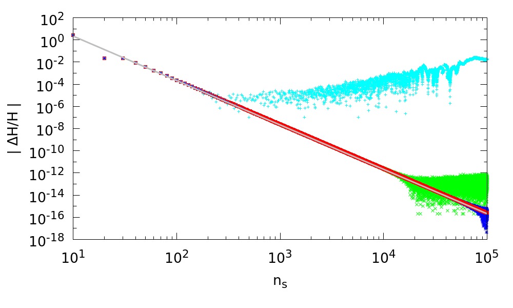
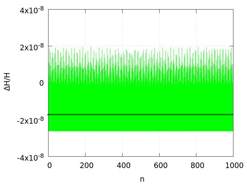
Figure 1: Integration error and variation of $H$. Left: variation of the first integral $H$ (in the rotating frame Hamiltonian) $|\Delta H/H|$ in one period $T$, as a function of the number of integration steps per period $n_{s}$. Results for different machine precision are compared: single (cyan), double (green), extended (blue) and quadruple precision (red). The integrations are based on a fourth order symplectic scheme for the Hamiltonian $H_{F}$, see equation 1, with time step $\Delta t=T/n_{s}$. The error saturates when the machine accuracy is reached. The gray line is the linear ln-ln fit $|\Delta H/H|=c\,n_{s}^{-\gamma}$ where $\gamma=-4$ within the statistical errors. The initial conditions are chosen for a regular orbit, with initial conditions $x(0)=0.55$, $y(0)=0$, $\dot{x}(0)=0$ and $\dot{y}(0)$ defined by the value of the Jacobi constant set up equal to $J=3.07$. Right: variation of $|\Delta H|$ along the orbit $M^{n}({\bf x}_{0})$. Even though $\Delta H$ fluctuates, its average vanishes.

If we choose $n_{s}$ below this threshold then the value of the first integral along the orbit of the map oscillates without growing. A power law fit to the growth of $(\Delta H)_{n}=|H\left(M^{n}({\bf x}_{0})-H({\bf x}_{0})\right)|$ with the number of periods $(\Delta H)_{n}=C\,n^{\beta}$ gives $\beta=0$ within the numerical uncertainties, see figure 1 right. This is true as long as the error growth due to the round-off is negligible. To evaluate the dynamic stability of the map we consider its perturbation $M_{\epsilon}$ and look at two different type of errors: the distance $d_{n}$ of the perturbed orbit from the reference one and the variation $(\Delta H)_{n}$ of the first integral along the perturbed orbit. We compare this error with the reversibility error $d^{(R)}_{n}$ and $(\Delta H)_{n}^{(R)}$. In the case of round-off we have access only to the reversibility error. In the case of random errors the numerical simulations support the asymptotic equivalence of the forward and reversibility errors, which in the previous section was proved to hold for linear symplectic maps. In addition the asymptotic behavior of reversibility errors looks very similar for round-off and random perturbations, when a single realization is considered. In the case of random errors a smooth behavior is obtained averaging over many realizations and a good agreement with the theoretical predictions is obtained. For the round-off different hardwares give different results with variations very similar to the ones obtained for different realizations of random perturbations. The reversibility error for $n=1$ (the application of the one period map and its inverse) due to round-off is almost independent on the number $n_{s}$ of steps per period, in a wide range $10\leq n_{s}\leq 10^{4}$, and it is close to the machine accuracy. This is due to the use of symmetric and symplectic integrator. The numerical analysis we present refers to the map which integrates the Hamiltonian $H_{F}$ in the fixed frame, choosing the mass ratio $\mu=0.000954$ (close to the Jupiter-Sun case). The initial conditions are chosen in the rotating frame for the same value of the Jacobi constant $J=3.07$ (on the Lagrange point $L_{4}$ we have $J=J_{c}\equiv 2.9990468$). We choose $y(0)=\dot{x}(0)=0$ and $x(0)=0.55$, as initial conditions for a regular orbit and $x(0)=0.56$ for a chaotic orbit. The value of $\dot{y}(0)>0$ is fixed by equation 7. In 6 we show the phase portrait of these orbits and nearby ones on the Poincaré manifold ${\cal M}_{P}$ projected on the $\left(x,\dot{x}\right)$ phase plane.

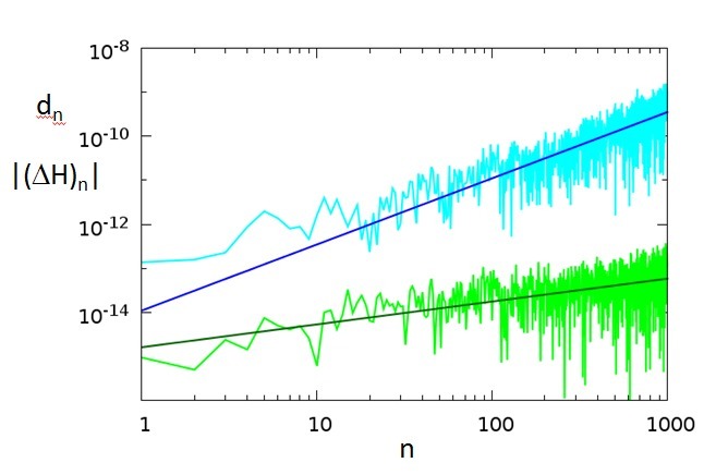
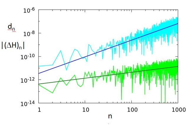
Figure 2: REM errors and power law fit for a regular orbit Left panel: evolution of the Reversibility Error $d_{n}^{(R)}$ (cyan) and $(\Delta H)^{(R)}_{n}$ (green) due to the round-off computed for a regular orbit with initial condition $x(0)=0.55$ and $y(0)=\dot{x}(0)=0$ the value of $\dot{y}(0)>0$ is fixed by equation 7. The straight blue line is the least squares fit to $d_{n}^{(R)}=Cn^{\beta_{d}}$. The dark-green line is the least squares fit to $(\Delta H)_{n}^{(R)}=Cn^{\beta_{H}}$. The exponents are $\beta_{d}=1.50\pm 0.09,\,\,\beta_{H}=0.52\pm 0.1$. Right panel: evolution of the reversibility error for a stochastic perturbation of amplitude $\epsilon=10^{-13}$. The straight lines correspond to the least squares fit with $\beta_{d}=1.43\pm 0.09,\,\,\beta_{H}=0.5\pm 0.1$. The interval where the fit is computed is $50\leq n\leq 1000$.

In figure 2 we show, for the regular orbit, the plot of the REM errors $d^{\,(R)}_{n}$ and $(\Delta H)_{n}^{(R)}$ for the round-off (left panel) and for a random perturbation (right panel). The computations are in double precision so that the round-off error amplitude is $\epsilon\sim 10^{-16}$ whereas the random perturbation amplitude is $\epsilon=10^{-13}$. In all the figures the time step is fixed to $n_{s}=1000$. In figure 3, for the same orbit, we show the plot of forward global errors FEM $d_{n}$ and $(\Delta H)_{n}$ for the same random perturbation, after averaging on $100$ realizations (left panel) and the Lyapunov global error LEM (right panel). The initial condition for LEM is varied according to $x(0)+\epsilon$ with $\epsilon=10^{-13}$. The error growth follows a power law

$$d_{n}\sim\epsilon\,n^{\beta_{d}}\qquad\qquad(\Delta H)_{n}\sim\epsilon\,n^{\beta_{H}}$$ (30)

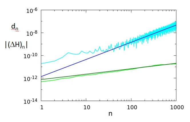
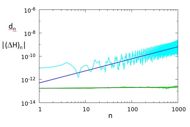
Figure 3: FEM and LEM errors and power law fit for a regular orbit. Left panel: evolution of the Forward Error $d_{n}$ (cyan) and $(\Delta H)_{n}$ (green) due to a random perturbation of amplitude $\epsilon=10^{-13}$ with $100$ realizations of the noise for the regular orbit with initial condition $x(0)=0.55$. The straight lines are the least squares fit with $\beta_{=}1.51\pm 0.05$ (blue) and $\beta_{H}=0.48\pm 0.01$ (dark-green). Right panel: evolution of the Lyapunov Error $d_{n}$ and $(\Delta H)_{n}$ with a perturbation to the initial condition $x(0)+\epsilon$ with $\epsilon=10^{-13}$. The straight lines correspond to the least squares fits with $\beta_{d}=1.04\pm 0.07,\,\,\beta_{H}=0.03\pm 0.01$. This low value of $\beta_{H}$, though not zero (three standard deviations are required to reach it), is explained as the round-off effect which start to be appreciable precisely around $n=1000$. The interval where the fit is computed is $50\leq n\leq 1000$. The round-off error rises as $10^{-15}(nT)^{1/2}$ and for $n=1000$ becomes appreciable.

For an integrable map the theoretical prediction for REM and FEM errors due to a random perturbation is $\beta_{d}=3/2$ and $\beta_{H}=1/2$, whereas $\beta_{d}=1$ and $\beta_{H}=0$ for the Lyapunov error. The straight lines in the figures are obtained by least squares fits. In the table 1 we quote the corresponding values of the exponents $\beta_{d}$ and $\beta_{H}$. For the round-off the value of $\beta_{d}$ is compatible $3/2$ and the value of $\beta_{H}$ is compatible with $1/2$, which are theoretically predicted for the random perturbations. The variations of the exponents with different hardware implementations of the round-off are similar to the changes observed between different realizations of random perturbations.

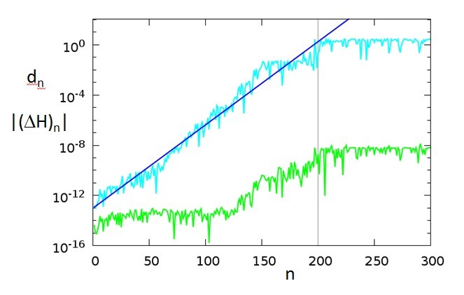
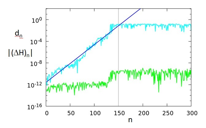
Figure 4: REM errors and power law fit for a chaotic orbit. Left panel: evolution of the Reversibility Error $d_{n}$ (cyan) and $(\Delta H)_{n}$ (green) due to round-off computed for a chaotic orbit with initial condition $x(0)=0.56$. The straight line corresponds the least squares fit with $\beta_{d}=0.0067\pm 0.002$. Right panel: evolution of the reversibility error for a stochastic perturbation of amplitude $\epsilon=10^{-13}$. The straight line corresponds to the least squares fit with $\beta_{d}=0.071\pm 0.003$. The fitting interval $1\leq n\leq 200$ for the left panel, $1\leq n\leq 150$ for the right panel.

In figure 4 we show the plot of REM errors due to the round-off (left panel) and to a random perturbation (right panel) for a chaotic orbit. In figure 5 the plot of the FEM error for a random perturbation (left panel) and LEM error (right panel) is shown for the same chaotic orbit. In this case the growth of the distance is exponential

$$d_{n}\sim\epsilon\,10^{\beta\,n}\qquad\qquad\lambda={\beta\over T}\ln 10$$ (31)

where $\lambda$ is the maximum Lyapunov exponent. The orbits have been computed up to $n=300$ periods. Notice that REM with round-off saturates at $n\sim 200$ whereas REM and FEM errors for stochastic perturbations and LEM saturate at $n\sim 150$. This is easily explained if we notice that in the first case $\epsilon\sim 10^{-16}$, whereas in the second case $\epsilon\sim 10^{-13}$. The least squares fit gives $\beta_{d}=0.07$ which corresponds to $\lambda\sim 0.0256$, in good agreement with the value obtained for the maximum Lyapunov exponent $\lambda$ computed with the renormalization method, which avoids saturation.

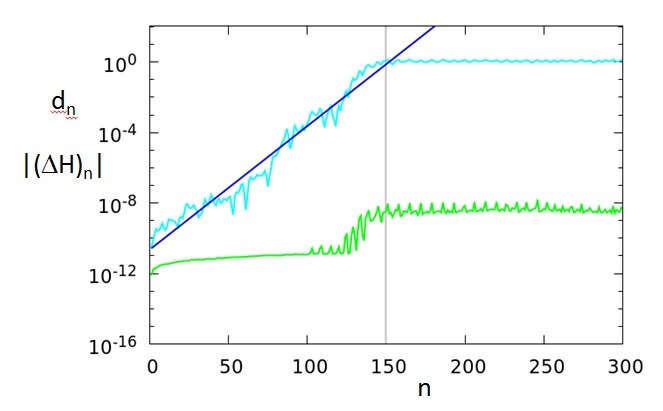
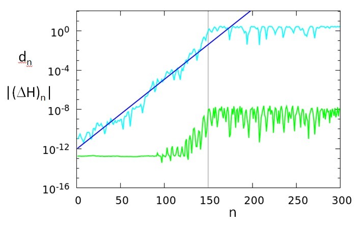
Figure 5: FEM and LEM errors and power law fit for a chaotic orbit. Left panel: evolution of the Forward Error $d_{n}$ (cyan) and $(\Delta H)_{n}$ (green) due to a random perturbation of amplitude $\epsilon=10^{-13}$ with $100$ realizations of the noise for the chaotic orbit $x(0)=0.56$. The straight line is the least squares fit with $\beta_{d}=0.070\pm 0.002$. Right panel evolution of the Lyapunov Error with a perturbation to the initial condition $x(0)+\epsilon$ where $\epsilon=10^{-13}$ The straight lines corresponds to the least squares fit with $\beta_{d}=0.071\pm 0.002$. The fitting interval is $1\leq n\leq 150$.

Also in this case the REM error due to round-off and stochastic perturbations exhibit the same behavior. The error on the first integral $H$ remains constant for a while, then has an exponential growth with about the same coefficient $\beta_{H}=0.07$ and saturates to a value close to the variation $\Delta H$ of the first integral $H$ along the unperturbed orbit due to the truncation error. In the table 1 we resume the values of the exponents obtained by fitting the global error data for FEM, REM and LEM.

Regular orbit	REM round-off	REM stochastic	FEM stochastic	LEM
$\beta_{d}$	$1.50\pm 0.09$	$1.43\pm 0.09$	$1.51\pm 0.05$	$1.04\pm 0.07$
$\beta_{H}$	$0.52\pm 0.1$	$0.5\pm 0.1$	$0.48\pm 0.01$	$0.03\pm 0.01$

Chaotic orbit	REM round-off	REM stochastic	FEM stochastic	LEM
$\beta_{d}$	$0.067\pm 0.002$	$0.071\pm 0.003$	$0.070\pm 0.002$	$0.071\pm 0.002$

Table 1: Table of exponents. The exponents of the power law for regular orbits and of the exponential law for chaotic orbits obtained by fitting the simulation results for REM, FEM and LEM errors are presented.

Phase space REM plots

The geometry of orbits is usually inspected by considering the Poincaré map $M_{P}$ on the 2D manifold ${\cal M}_{P}$. The orbits are visualized by projecting them into the $\left(x,\dot{x}\right)$ phase plane. In this case the machine accuracy is not required for the intersection and a linear interpolation is adequate.

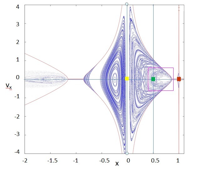
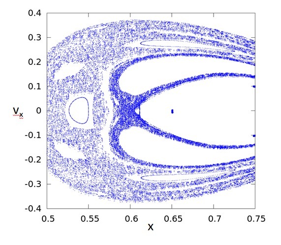
Figure 6: Poincaré map with a zoom. Left panel: projection on the phase plane $(x,v_{x}=\dot{x})$ of several orbits of the Poincaré map on ${\cal M}_{P}$. The time step is ${\Delta t}=T/n_{s}$ with $n_{s}=1000$. The Sun, Jupiter and the Lagrange point $L_{4}$ are indicated by a yellow, brown and green square respectively. The blue horizontal line is the $x$-axis and the vertical one is parallel to the $y$-axis and passing trough the $L_{4}$ Lagrangian point. The orbits are within a region, whose boundary is delimited by red lines defined according to equation 6 by $v_{x}=\pm\,\sqrt{x^{2}+2(1-\mu)/|x+\mu|+2\mu/|x-1+\mu|-J}$. Right panel: magnification of the region delimited by the purple box in the left panel.

The dynamic stability can be analyzed by considering the error on a set of points of ${\cal M}_{P}$ for a fixed value $n$ of iterations of the Poincaré map. If we consider the reversibility error no intersection of the orbit with the manifold ${\cal M}_{P}$ is required, since we start from an initial point in ${\cal M}_{P}$ and come back to it up to an error due to the round-off or random perturbation. Since for a chaotic orbit the error saturates to $1$ after a few hundreds iterations, the choice $n=100$ is already adequate to distinguish regions of regular and chaotic behavior, where the error is separated by many orders of magnitudes. The REM error is computed in a grid of points selected in a rectangular domain of the $\left(x,\dot{x}\right)$ plane to which corresponds a domain in ${\cal M}_{P}$ having fixed the value $J$ of the Jacobi invariant. This method is fast and can be compared, in terms of speed, with the fast Lyapounov indicator (FLI, [29]), but its remarkable propriety is that it can be used to estimate the global error due to the round-off.

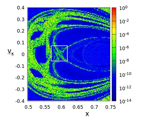
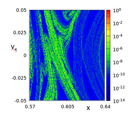
Figure 7: REM color map. Left panel: the Reversibility Error due to round-off for the one period map $M$. The time step is ${\Delta t}=T/n_{s}$ with $n_{s}=1000$. The number of periods for the computation of the REM is $n=1000$. A color scale is used for the points in a regular grid chosen in the same region of the $(x,v_{x}=\dot{x})$ phase plane as in the right panel of figure 7. The presence of regions of regular and chaotic motion appears neatly. On the region of regular motion the error is close to the round-off. On the region of chaotic orbits the error is close to $1$. Right panel: the magnification of a transition region corresponding to the white box in the left panel.

In figure 6 we present a portrait of the whole phase space, delimiting with red lines the allowed region, defined by equation 6, and its magnification. In figure 7 we show the plot, using a color scale, of the REM error for the round-off with $n=1000$ iterations of the one period map. The chosen phase space region is the same as in figure 6 right panel. A new magnification is also shown on the right panel, corresponding to the white box on the left panel. The REM color plot allows a rapid and effective visualization of the dynamic stability of the system with respect to random perturbations, and requires only few lines of code for a given symplectic integrator. For the round-off or random perturbations the REM plot requires a moderate CPU time even on a fine grid, since the number $n$ of iterations is low.

5 Fidelity

The speed at which the dynamic evolution looses memory of the initial condition is measured by the correlation decay rate. Given an orbit ${\bf x}_{n}=M^{n}({\bf x})$, where $M$ is a symplectic map and $f({\bf x})$ is an observable (dynamic variable), one defines the correlation according to

$$\hat{C}(n)=<f(M^{n})f>-<f>_{\mu}<f>$$ (32)

$$C(n)=<f(M^{n})f>-<f(M^{n})><f>$$

Though these definitions are equivalent in the limit $n\to\infty$, only the second one is suitable for numerical computations. The averages are defined according to

$$<f>=\int_{\cal E}f({\bf x})dm({\bf x})\qquad\qquad<f>_{\mu}=\int_{\cal E}f({\bf x})d\mu({\bf x})\equiv\lim_{n\to\infty}\int_{\cal E}f(M^{n}({\bf x}))\,dm({\bf x})$$ (33)

where $m({\bf x})$ denotes the normalized Lebesgue measure. We denote by $m_{L}$ the Lebesgue measure; for example $\mu_{L}({\cal B})$ is the area of ${\cal B}$ if ${\cal B}\in{R}^{2}$ and the volume of ${\cal B}$ if ${\cal B}\in{R}^{4}$. If ${\cal E}$ is an invariant domain of phase for any ${\cal B}\subset{\cal E}$ the measure $m$ is defined by

$$m({\cal B})={m_{L}({\cal B})\over m_{L}({\cal E})}$$ (34)

The invariant measure has the following property

$$\mu(M^{-1}({\cal B}))=\mu({\cal B}).$$ (35)

If the map is symplectic then its inverse is unique. In this case the invariance condition in this case reads $\mu(M^{-1}({\cal B}))=\mu(M({\cal B}))=\mu({\cal B})$. For the one period map the phase space is ${R}^{4}$. If we consider an initial set ${\cal A}_{0}\subset{R}^{4}$ the invariant manifold ${\cal E}$ is the union of all the forward images of ${\cal A}_{0}$. Remark that ${\cal A}_{0}$ can be reduced to a single point, in which case ${\cal E}$ is just the orbit having this point as initial condition. The Lebesgue measure is just the volume so that

$${\cal E}=\cup_{n=0}^{\infty}M^{n}({\cal A}_{0})\qquad\qquad\mu({\cal B})={\,\hbox{Vol}\,({\cal B})\over\,\hbox{Vol}\,({\cal E})},\,\qquad{\cal B}\subset{\cal E}.$$ (36)

We may compute the fidelity for the one period map, which is the Poicaré map $\tau=0\,\hbox{mod}\,2\pi$ for the Hamiltonian $H_{F}$ in the fixed frame. It is computationally more convenient to consider the Poincaré map $y=0,\,\,p_{y}>0$ for the Hamiltonian $H$ in the rotating frame. This is a map define on the 2D manifold ${\cal M}_{P}$ and its projection on the $\left(x,\dot{x}\right)$ or $\left(x,p_{x}\right)$ phase plane has an invariant measure $\mu$ given by the normalized area with respect to an invariant domain ${\cal E}$. Typically, ${\cal E}$ is the closure of an orbit issued from a given point or the union of the images of a given domain, which numerically is sampled with a finite set of points. If the points of the orbit ${\bf x}_{0},{\bf x}_{1},\ldots,{\bf x}_{n}$ were random independent variables, the correlation would vanish for any $n$. For a deterministic Hamiltonian system the correlation does not decay or decays as $n^{-1}$ for regular orbits whereas it decays exponentially fast to zero for chaotic orbits. If the system is perturbed deterministically, stochastically or by round-off the perturbed orbit looses memory of the unperturbed one. The Fidelity is defined as the correlation between the unperturbed orbit and the perturbed one after $n$ iteration of the perturbed map according to

$$\hat{F}_{\epsilon}(n) =<f(M^{n})f(M_{{\,\epsilon}}^{n})>-<f>_{\mu}<f>_{\mu_{{\,\epsilon}}}$$ (37)

$$F_{\epsilon}(n) =<f(M^{n})f(M_{{\,\epsilon}}^{n})>-<f(M_{\,\epsilon}^{n})><f(M^{n})>$$

where $\mu_{\,\epsilon}$ is the invariant measure associated to the perturbed map $M_{\,\epsilon}$, namely the stationary measure in the case of random perturbations. For Hamiltonian systems the invariant and the stationary measures are equal to the normalized Lebesgue measure $\mu_{\epsilon}=\mu=m$ so that there is a unique definition (also for the correlation) and the term to be subtracted in equation 37 is $\langle\,f\,\rangle^{2}$. Another definition of Fidelity (related to REM), for symplectic maps, is the following

$$F^{(R)}_{\epsilon}(n) =<f(M_{{\,\epsilon}}^{-n}\circ M_{{\,\epsilon}}^{n})\,\,f>-<f>^{2}$$ (38)

For regular maps such as translations on the torus ${{T}}^{d}$ the correlations and the Fidelity do not decay. For anisochronous maps on the cylinder ${{C}}={{T}}^{d}\times{{I}}$ (where ${{I}}$ is a pluri-interval in ${R}^{d}$ to which the actions belong) the correlations and the Fidelity decay as $1/n$ for observables whose average on every torus is the same. This behavior is typical of integrable systems. For random perturbations depending on ${\,\epsilon}{\mathchar 28952\relax}$ where ${\mathchar 28952\relax}$ is a vector of independent random variables with zero mean and unit variance, the Fidelity of $M_{\,\epsilon}$ with respect to $M$ decays exponentially if $M$ is a regular map

$$F_{\epsilon}(n)\sim e^{-d_{n}^{2}}\sim\exp\left({{-c\,\epsilon^{2}n^{2\beta}}}\right)$$ (39)

where the exponent $\beta$ is $3/2$ for a generic observable. For an isochronous system where the angle is stochastically perturbed the exponent is $\beta=1/2$. For chaotic maps the Fidelity decays as

$$F_{\epsilon}(n)\sim e^{-d_{n}^{2}}\sim\exp\left({{-c\,\epsilon^{2}10^{2n\beta}}}\right)$$ (40)

If $M$ is the one period map we have $\beta=\lambda\,\,T/\ln 10$ where $\lambda$ is the maximum Lyapunov exponent. If we choose $M$ equal to the one step map $M_{\Delta t}$ then $\beta=\lambda\,{\Delta t}/\ln 10$. If $M$ is the Poincaré map the time between two intersections is comparable with $T$ so that $\beta\sim\lambda\,\,T\ ln(10)$. The Fidelity exhibits a plateau extending from $n=0$ to $n=n_{*}$ defined by

$$n_{*}={\ln\,{\,\epsilon}^{-1}\over\beta\,\ln 10}$$ (41)

followed by a super-exponential decay. These results where proved for linear maps on the torus and the cylinder with additive noise $M_{\,\epsilon}=M+{\,\epsilon}\xi$ [19]. Rigorous results in a more general setting for deterministic perturbations were obtained for chaotic maps with exponentially decaying correlations [18]. If the perturbation is due to the round-off then the Fidelity does not decay for regular maps such as the translations on the torus ${{T}}^{d}$. If the perturbation is a frequency shift linearly depending on the action, the Fidelity decays as $1/n$. The Fidelity behavior when the perturbation is due to the round-off changes drastically for an integrable system if action angle or Cartesian coordinates are used. In the first case the forward and reversibility error do not grow and the Fidelity does not decay. In the second case the error grows with a power law whose exponent is $\beta=1/2$ if the map is isochronous, $\beta=3/2$ if it is anisochronous. Correspondingly the Fidelity has an exponential decrease with the same exponent $\beta$. When Cartesian coordinates are used the map is computationally complex enough that round-off and random perturbations produce the same effect. In action angle variables the round-off is ineffective whereas the random perturbations cause a power law growth of the global error and an exponential decay of Fidelity according to equations 39 and 40. We have checked numerically this behavior for harmonic and anharmonic oscillators. Non-integrable Hamiltonians exhibit both regular and chaotic orbits. The Fidelity decay is exponential an super-exponential respectively and the decay law is the same for the round-off and random perturbations [21], [22] in agreement with the same exponential growth of the global error described in the previous section. For the $3$-body problem we have computed the Fidelity for the Poincaré map in the rotating system because it is 2D using stochastic perturbations of amplitude $\epsilon>10^{-6}$. In this case linear interpolation can be used since the error it involves is at least 4 orders of magnitude below the random error (the use of the Hénon method is not straightforward since the integration is carried out in the fixed reference frame).

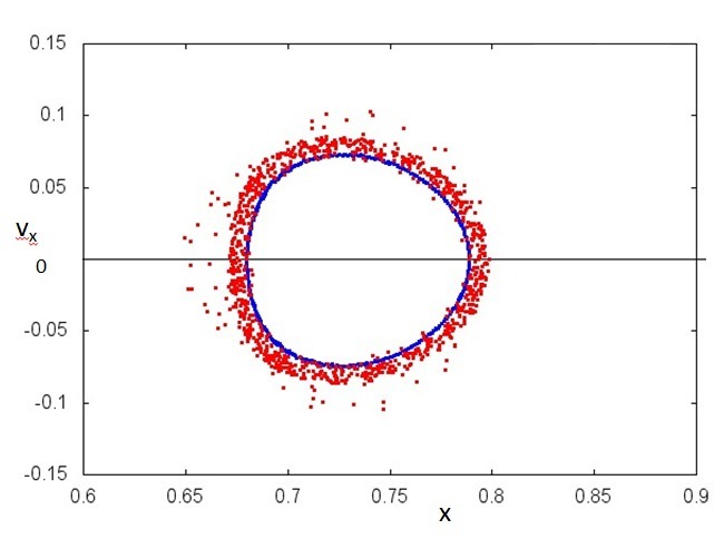
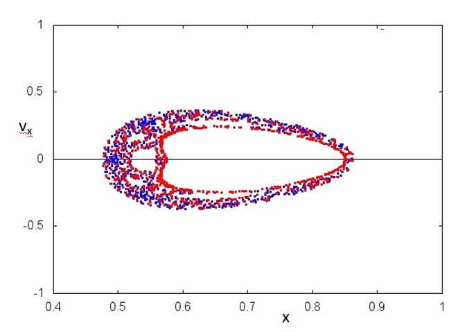
Figure 8: Unperturbed and noisy orbits. Left panel: projection on the $(x,v_{x}=\dot{x})$ phase plane of a regular orbit in the Poincaré section ($y=0$, $\dot{y}=0$) with a stochastic perturbation of amplitude ${\,\epsilon}=10^{-3}$ (red dots). The initial point is $x(0)=0.68$ and $\dot{x}=0$ in the Jacobi manifold $J=3.07$. The unperturbed orbit is also shown (blue dots). Right panel: chaotic orbit with initial points $x(0)=0.56$ (blue dots). The orbit with a stochastic perturbation of amplitude ${\,\epsilon}=10^{-4}$ is shown (red dots).

The Jacobi manifold is defined by $J=3.07$ and the section half plane is $y=0,\,\dot{y}>0$. The symplectic perturbation in this case is introduced in the second order integrator $M^{(2)}_{{\Delta t}}=I+{\Delta t}\,N$ by modifying it into $M^{(2)}_{{\,\epsilon},{\Delta t}}=I+{\Delta t}N(1+\epsilon_{0}{\mathchar 28952\relax})$. By composing three second order maps the fourth order symplectic map $M^{(4)}_{{\,\epsilon},{\Delta t}}$ is obtained and the Poincaré map $M$ is computed. If ${\Delta t}=T/n_{s}$ then the number of iterations from two subsequent sections is comparable with $n_{s}$. We have chosen $n_{s}=100$. The random vector was changed only after each section and kept constant until the next section; changing it at every time step produced no significant difference.

We have analyzed the Fidelity for two distinct initial conditions on the Poincaré section: $x(0)=0.68$ for a non resonant orbit diffeomorphic to a circle, and $x(0)=0.56$ for chaotic orbit. The initial point $x(0)=0.55$ considered in the previous section belongs to a stable resonant orbit formed by three islands. The orbits in the phase plane $\left(x,\dot{x}\right)$ with and without the stochastic perturbation are shown in figure 8.
For the regular orbit we consider a sequence of values of the noise amplitude ${\,\epsilon}_{0}=2^{1-m}\,10^{-3}$ for $0\leq m\leq 4$. The effective perturbation of the map is $\epsilon_{0}\,{\Delta t}=\epsilon_{0}\,2\pi/n_{s}$. The Fidelity exhibits an exponential decay which can be fitted by

$$F_{\epsilon}(n)=F_{\epsilon}(0)\exp(-C({\,\epsilon})\,n^{3}).$$ (42)

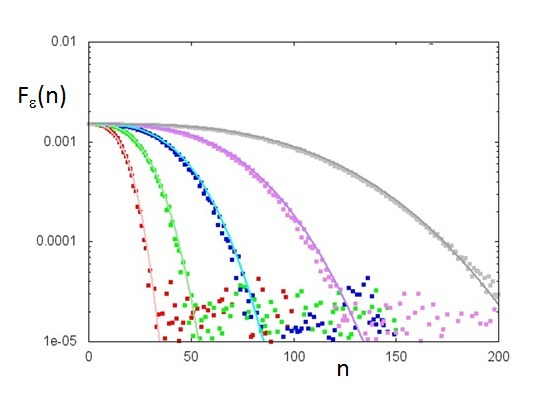
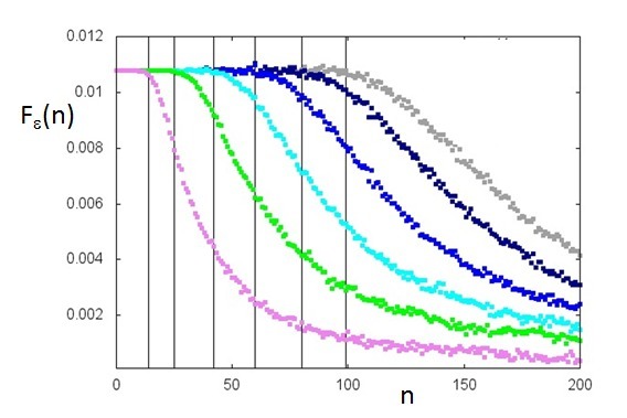
Figure 9: Fidelity for a regular and chaotic orbit with noise. Left panel: plot of the Fidelity $F_{\,\epsilon}(n)$ for the observable $f=x$ in the case of a regular orbit with initial point $x(0)=0.68$ and $\dot{x}(0)=0$, stochastically perturbed. The small squares are the results of simulations with different values of the stochastic perturbation amplitude: ${\,\epsilon}=2\,10^{-3}$ red squares, ${\,\epsilon}=10^{-3}$ green squares, ${\,\epsilon}=5\,10^{-4}$ blue squares, ${\,\epsilon}=2.5\,10^{-4}$ purple squares, ${\,\epsilon}=1.25\,10^{-4}$ gray squares. The number of steps per period for the symplectic fourth order integrator is $n_{s}=100$. The number of realizations of the stochastic perturbation is $N=100$. The continuous lines are the fits according to equation $exp(-C({\,\epsilon})n^{2\beta})$. The fitted coefficients $C({\,\epsilon})$ exhibit a quadratic dependence on ${\,\epsilon}$ namely $C({\,\epsilon})=c{\,\epsilon}^{2}$ in agreement with equation 39. Right panel: plot of the Fidelity $F_{\,\epsilon}(n)$ for a chaotic orbit with initial point $x(0)=0.56$, $\dot{x}(0)=0$ stochastically perturbed. The perturbation amplitude is: ${\,\epsilon}=10^{-4}$ purple squares, ${\,\epsilon}=10^{-6}$ green squares, ${\,\epsilon}=10^{-8}$ cyan squares, ${\,\epsilon}=10^{-10}$ blue squares, ${\,\epsilon}=5\,10^{-12}$ dark blue squares, ${\,\epsilon}=10^{-14}$ gray squares. The vertical lines correspond to the end of the plateaus $n_{*}(\epsilon)$, which depend linearly on $\ln(1/\epsilon)$.

In figure 9 left we show the Fidelity for the observable $f({\bf x})=x$ and the result of a least squares fit according to equation 42. The coefficients $C(\epsilon)$ obtained from the fit exhibit a quadratic dependence on $\epsilon$ according to $C({\,\epsilon})=c{\,\epsilon}^{2}$ with $c\simeq 30$. In a previous paper [19], the decay rate $\exp(-{\,\epsilon}^{2}\,n^{3})$ was proved to occur for a stochastically perturbed map of the cylinder for an observable $f(\theta)$ where $\theta$ is the angle variable. In the $3$-body problem the unperturbed orbit is close to a circle and the radial diffusion of the perturbed orbit shows that the perturbation affects also the action variable $\jmath$. As a consequence since $x\simeq(2\jmath)^{1/2}\,\cos\theta$ the observed decay law is compatible with the result proven for the stochastically perturbed map of the cylinder. For the chaotic orbit we compute the Fidelity for the sequence of values of the noise amplitude ${\,\epsilon}_{0}=10^{-2m}$ for $2\leq m\leq 7$ though only for $m\leq 4$ the error in the linear interpolation can be safely neglected. In figure 9 right we show the plots of the Fidelity $F_{\epsilon}(n)$. For any value of ${\,\epsilon}$ the Fidelity exhibits a plateau up to a value $n_{*}({\,\epsilon})$. The plateaus followed by a super-exponential decay are observed in other chaotic maps and the result was rigorously proved for the Bernoulli maps [19], where $n_{*}$ was given by equation 41. In the present case the growth of $n_{*}$ is linear with $\ln(1/{\,\epsilon})$ to a very good approximation.

6 Conclusions

In this paper we have applied the Reversibility Error Method (REM) and the Fidelity analysis to investigate the dynamic stability of the restricted three body problem. The perturbation is due either to the round-off or to random errors. The combined use of REM and Fidelity appears to be adequate to explore the dynamical features on a given invariant Jacobi manifold. The reversibility error provides asymptotically the same information as the forward error but does not require the exact computation of the unperturbed orbit. Therefore, is well suited to inspect the effect of round-off. The loss of memory of the perturbed orbit it is measured by the Fidelity decay whose computation requires a Monte-Carlo sampling of the unperturbed orbits. The round-off appears to produce the same effects as random perturbations, if a single realization is considered, provided that the map is sufficiently complex from the computational viewpoint. In the case of random perturbations a smoother asymptotic behavior of the error is achieved by averaging over several realizations. The computation of the reversibility error for a fixed number of iterations on a grid of points on a 2D manifold, combined with a color plot for visualization, is a straightforward procedure which allows to explore the dynamic stability of the map, especially in the transition regions. To distinguish regular from chaotic orbits very low value of $n$ can be used ($n<100$) just as for the Fast Lyapounov Indicator (FLI). The maximum Lyapunov exponents and related indicators require more elaborate algorithms and extrapolations to infinity. The remarkable property of the REM method allow to quantify the global error due to the round-off. The Fidelity is computationally expensive but provides statistical information. For regular orbits with a random perturbation of amplitude $\epsilon$ the REM and FEM global errors growth follows a power law $\epsilon\,n^{\beta}$ whereas the Fidelity exhibits an exponential decay $e^{-c\,\epsilon^{2}\,n^{2\beta}}$. For chaotic orbits with a random perturbation the REM and FEM global error growth is $\epsilon\,\,{10}^{n\,\beta}$, whereas the Fidelity decay is $\exp(-c\,\epsilon^{2}\,\,{10}^{2n\beta})$. For the symplectic map used to integrate the $3$-body problem the asymptotic behavior of REM and FEM global errors due to a random perturbation and the corresponding decay of Fidelity are fully confirmed. We have observed that the REM global errors growth and the Fidelity decay for the round-off are asymptotically the same as for random perturbation, even though the uncertainty on the exponent $\beta$ is larger. This result is expected if the map is complex enough from the computational viewpoint. For an integrable system the result is different when action angle variables are used, since the computational complexity is too low. Indeed with round-off the REM error vanishes and the Fidelity does not decay, whereas with a random perturbation the previous scaling laws are satisfied. To summarize we claim that REM and Fidelity appear to be adequate to analyze the dynamic stability of non-integrable systems with a few degrees of freedom. Their use may be recommended to explore the transition regions where regular and chaotic dynamics coexist and their relative weight affects the statistical properties, as observed and proved for simple models, in the case of Poincaré recurrences [30]. The results obtained for the $3$-body problem suggest the application of REM and Fidelity to the few body problem as the next natural step. The few body problem is a key issue in the description of observed exo-planets ([31]). Indeed the stability of planets in the habitable zone is a necessary, tough not sufficient, condition for the existence of extraterrestrial life [32], [33]. The presence of MMRs can stabilize or destabilize the orbit of a planet and the consequent evolution of the planetary system (see for instance [34]). The recent progress in the field of planetary science, due to the Kepler [35] and GAIA missions [36], give the opportunity to test a lot of planetary systems including resonant or quasi-resonant exo-planets ( see [37] for a review of known resonant or quasi resonant extra-solar systems). Other fields of astrophysics which might benefit of the proposed approach are the characterization of regular and chaotic orbits in elliptical galaxies [38], the motion of binary black holes at the centre of galaxies [39] and generic Hamiltonian astrophysical systems (for example [40], [41] and reference therein). One of the future and relevant application in astrophysics is the study of stochastic orbits in axial-symmetric potentials built with the technique of holomorphic shift [42].

Appendix A Error analysis for 2D linear symplectic maps

We consider the case of a $2\times 2$ symplectic matrix $A$ distinguishing three possible cases: I) If $|\,\hbox{Tr}\,(A)|>2$ the eigenvalues are real and $A=U\Lambda U^{-1}$ where $\Lambda=\hbox{diag}\,(e^{\lambda},e^{-\lambda})$. Choosing $\det U=1$ we introduce the positive matrix

$$V=U^{T}U=\begin{pmatrix}a&b\\ &\cr b&c\end{pmatrix}\qquad\qquad a,c>0\qquad ac-b^{2}=1$$ (43)

The traces of $A^{k}\,(A^{k})^{T}$ and $V\Lambda^{k}\,V^{-1}\Lambda^{k}$ are equal and we obtain the asymptotic behavior of $d_{n}$ according to

$$\,\hbox{Tr}\,(A^{k}\,(A^{k})^{T})=ac\,e\,^{2k\lambda}+ac\,e^{-2k\lambda}-2b^{2}\qquad\quad\longrightarrow\qquad\quad d_{n}=C\,\,\epsilon\,e^{n\lambda}+O(n\,e^{-\lambda n})$$ (44)

where $C=(ac)^{1/2}\,(1-e^{-2\lambda})^{-1/2}$. This asymptotic approximation to $d_{n}$ is valid only for $\lambda$ sufficiently greater than zero. Taking the limit $\lambda\to 0$ in the exact expression for $d_{n}$ we have $d_{n}=\sqrt{2}\,\epsilon\,n^{1/2}$. II) If $|\,\hbox{Tr}\,(A)|<2$ the eigenvalues are complex of unit modulus $e^{\pm i\omega}$ so that we can write $A=UR(\omega)U^{-1}$ where $R$ is the rotation matrix and $U$ is a real matrix real. Still using the matrix $V=U^{T}\,U$ introduced above we evaluate the trace of $A^{k}\,(A^{k})^{T}$ and the asymptotic behavior of $d_{n}$ according to

$$\,\hbox{Tr}\,(A^{k}\,(A^{k})^{T})=2\,\cos^{2}(k\omega)+(a^{2}+c^{2}+2b^{2})\,\sin^{2}(k\omega)\quad\longrightarrow\quad d_{n}={a+c\over\sqrt{2}}\,\,\epsilon\,n^{1/2}+O(n^{-1/2})$$ (45)

III) If $TrA=2$ then either $A=I$ in which case $d_{n}=n^{1/2}$ or $A$ has the Jordan form $A=U\Lambda U^{-1}$ where $\Lambda=\begin{pmatrix}1&\alpha\\ 0&1\end{pmatrix}$. Using the matrix $V$ defined as above the trace of $A^{k}\,(A^{k})^{T}$ and the asymptotic behavior of $d_{n}$ is given by

$$\hskip-21.33955pt\,\hbox{Tr}\,(A^{k}\,(A^{k})^{T})=a^{2}\,\alpha^{2}\,k^{2}+2\quad\longrightarrow\quad d_{n}=\epsilon\,\left[{{{a^{2}\,\alpha^{2}\over 6}(2n^{3}+3n^{2}+n)+2n}}\right]^{1/2}={a\over\sqrt{3}}\,\,\alpha\,\,\epsilon\,n^{3/2}+O(n^{1/2})$$ (46)

The last two cases we have examined correspond to the behavior of an integrable map. In particular the second case corresponds to an isochronous map in cartesian coordinates, the third case to an anisochronous map in action angle coordinates (when $\alpha=0$ we recover the isochronous case in action angle coordinates). As a consequence the distance grows as $n^{1/2}$ for an isochronous system and as $n^{3/2}$ for an anisochronous system. The expression of $d_{n}^{(R)}$ define in equation 27 and using 44, 45 and 46 is immediately obtained. The sums in 27 entering the definitions of $(d_{n}^{(R)})^{2}$ and $(d_{n})^{2}$ give exactly the same results, since $A$ and $A^{-1}$ have the same eigenvalues. The contribution of $\,\hbox{Tr}\,[A^{-n}\bigl{(}A^{-n}\big{)}^{T}-I]$ does not change the leading term in the asymptotic expressions. As a consequence $d^{(R)}_{n}=\sqrt{2}\,\,d_{n}$ up to the remainder terms both in the expanding and the integrable case. For the round-off the distances $d_{n}$ and $d_{n}^{(R)}$ exhibit large fluctuations as in the case of random errors when a single realization is considered. The expressions for $(d_{n}^{(R)})^{2}$ and $(d_{n})^{2}$ given by equations 25 and 26 involve an average which reduced the fluctuations. If the map is computationally sufficiently complex then the asymptotic behavior of $d_{n}$ and $d_{n}^{(R)}$ for the round-off is the same and agrees with the one observed and theoretically predictable for random errors. To support the previous results on the 2D maps we propose a simple exercise for an integrable Hamiltonian ${\cal H}=2\pi\,H(p)$ in angle action coordinates $(\phi=2\pi x,\,p)$, The scaled system with coordinates $(x,p)$ and Hamiltonian $H(p)$ is defined on the cylinder ${T}\times{{I}}$ where ${T}$ is the interval $[0,1]$ with identified endpoints and ${{I}}=[0,a]$. The stochastically perturbed Hamiltonian is $H_{\epsilon}=H(p)+\epsilon_{0}p\xi_{x}(t)-\epsilon_{0}x\xi_{p}(t)$ where $\xi_{x}(t)$ and $\xi_{p}(t)$ are independent white noises. Letting $\Omega(p)=dH/dp$ the equations of motion and their solution, up to corrections of order $\epsilon_{0}^{2}$, are

$$\dot{x} =\Omega(p)+\epsilon_{0}\xi_{x}(t)\hskip 184.9429pt\dot{p}=\epsilon_{0}\xi_{p}(t)$$ (47)

$$x =x_{0}+\Omega(p_{0})\,t+\Omega^{\prime}(p_{0})\,\epsilon_{0}\,w_{1\,p}(t)+\epsilon_{0}w_{x}(t)\hskip 56.9055ptp=p_{0}+\epsilon w_{p}(t)$$

where $w(t)=\int_{0}^{t}\,\xi(s)\,ds$ denotes the Wiener noise and $w_{1}(t)=\int_{0}^{t}\,w(s)\,ds$. The result, based on the first order Taylor expansion of $\Omega(p)$, is valid as long as $\epsilon\,|w_{p}(t)|\ll p_{0}$ namely for $\epsilon t^{1/2}\ll p_{0}$. In this case the distance growth after averaging on the process is

$$\hskip-7.11317ptd(t)=\left[{{\Bigl{\langle}(x-\langle x\rangle)^{2}+(p-\langle p\rangle)^{2}\Bigr{\rangle}}}\right]^{1/2}=\epsilon_{0}\,\,\left[{{(\Omega^{\prime}(p_{0}))^{2}\,{t^{3}\over 3}+2t}}\right]^{1/2}$$ (48)

The map $M$ which integrates the previous equation is

$$x_{n}=x_{n-1}+\Omega(p_{n}){\Delta t}+\epsilon_{0}\sqrt{{\Delta t}}\,\xi_{x,\,n}\hskip 56.9055ptp_{n}=p_{n-1}+\epsilon_{0}\sqrt{{\Delta t}}\,\,\xi_{p,\,n}$$ (49)

where $\xi_{x,\,n},\,\xi_{p,\,n}$ are independent random variables with zero mean and unit variance. Notice that the amplitude of noise in the symplectic integrator is $\epsilon=\epsilon_{0}\,\,({\Delta t})^{1/2}$. The map is non linear but $DM=A$ is constant since $p_{n}=p_{0}$ on the unperturbed trajectory. As a consequence $DM=A$ has the Jordan form $A=\left(\begin{array}[]{cc}1&\alpha\cr 0&1\cr\end{array}\right)$ with $\alpha=\Omega^{\prime}(p_{0})\Delta t$. Letting ${\Delta t}\to 0$ keeping $t=n{\Delta t}$ finite the same result as 48 is obtained. The $n^{3/2}$ growth of the forward error due to round-off has been observed for an integrable system in the specific case of central motion with $-1/r$ potential [7] and explained by assuming that the round-off behaves as a random perturbation . For a generic system there is a smooth transition from the $n^{1/2}$ to the $n^{3/2}$ growth law as the anisochronicity increases continuously starting from zero. A power law approximation $d_{n}=c{\,\epsilon}\,n^{\gamma}$ using the least squares fit to $d_{n}$ given by equation 29 (which reduces to equation 45 in the isochronous case and to 46 in the anisochronous case) with $t=n{\Delta t}$, provides an exponent $\gamma(\alpha)$ which smoothly varies between the asymptotic values $1/2$ to $3/2$ with a transition at $\alpha\sim 1$. We have checked this numerically for the anharmonic oscillator whose Hamiltonian in Cartesian coordinates is $H=(p^{2}+x^{2})/2+\eta x^{4}/4$. Choosing $M$ to be the fourth order symplectic integrator map with a random perturbation we have computed with a least squares fit the power law exponent $\beta$ as a function of $\eta$ for the same initial condition $(x_{0},p_{0})$. The dependence of $\beta$ on the nonlinearity strength $\eta$ obtained by fitting the analytic expression $d_{n}$ given by equation 29 is quite similar. When the error is due to the round-off $\beta(\eta)$ has large fluctuations, just as for a single realization of random errors, but the asymptotic limits and the transition region are the same.

Appendix B Second order symplectic integrators

The coordinates and velocities transformation from the rotating to the fixed frame and vice versa read

$$\begin{pmatrix}x_{F}\\ y_{F}\\ \dot{x}_{F}\\ \dot{y}_{F}\end{pmatrix}=\begin{pmatrix}R(-t)&0\\ \\ -\dot{R}(-t)&R(-t)\end{pmatrix}\begin{pmatrix}x\\ y\\ \dot{x}\\ \dot{y}\end{pmatrix}\qquad\qquad\begin{pmatrix}x\\ y\\ \dot{x}\\ \dot{y}\end{pmatrix}=\begin{pmatrix}R(t)&0\\ \\ \dot{R}(t)&R(t)\end{pmatrix}\begin{pmatrix}x_{F}\\ y_{F}\\ \dot{x}_{F}\\ \dot{y}_{F}\end{pmatrix}.$$ (50)

For brevity we denote the previous transformations as

$${\bf{x}}(t)={\bf{R}}(t){\bf{x}^{F}}(t)\qquad\qquad{\bf{x}}^{F}(t)={\bf{R}^{-1}}(t){\bf{x}}(t)$$ (51)

The second order integrator of Hamilton’s equations in the fixed frame corresponding to the operator $e^{{\Delta t}/2\,D_{V_{F}}}\,e^{{\Delta t}\,D_{T}{T_{F}}}\,e^{{\Delta t}/2\,D_{V_{F}}}$ explicitly read

$$x_{F,\,k+1}=x_{k}+\left[p_{x\,F,\,k}\Delta t+f_{x}(x_{F,\,k},y_{F,\,k},\tau_{k})\frac{(\Delta t)^{2}}{2}\right]$$ (52)

$$y_{F,\,k+1}=y_{F,\,k}+p_{y\,k}\,\Delta t+f_{y}(x_{F,\,k},y_{F,\,k},\tau_{k})\frac{(\Delta t)^{2}}{2}$$

$$\tau_{k+1}=\tau_{k}+\Delta t$$

followed by

$$p_{x\,F\,k+1} =p_{x\,F,\,k}+\Bigl{[}f_{x}(x_{F,\,k},y_{F,\,k},\tau_{k})\;+\;f_{x}(x_{F,\,k+1},y_{F,\,k+1},\tau_{k+1})\Bigr{]}\frac{\Delta t}{2}$$ (53)

$$p_{y\,F,\,k+1} =p_{y\,F,\,k}+\Bigl{[}f_{y}(x_{F,\,k},y_{F\,k},\tau_{k})+f_{y}(x_{F,\,k+1},y_{F,\,k+1},\tau_{k+1})\Bigr{]}\frac{\Delta t}{2}$$

$$p_{\tau\,k+1} =p_{\tau\,k}+\Bigl{[}f_{\tau}(x_{F,\,k},y_{F\,k},\tau_{k})+f_{\tau}(x_{F,\,k+1},y_{F,\,k+1},\tau_{k+1})\Bigr{]}\frac{\Delta t}{2}$$

where $f_{x},f_{y},f_{\tau}$ are the derivative of $-V_{F}(x_{F},y_{F},\tau)$, defined in equation 1, with respect to $x_{F},y_{F},\tau$. The second order integrator of Hamilton’s equations in the rotating frame corresponding to the operator $e^{{\Delta t}/2\,D_{V}}\,e^{{\Delta t}\,D_{T}}\,e^{{\Delta t}/2\,D_{V}}$ explicitly read

$$\begin{pmatrix}x_{k+1}\\ \cr y_{k+1}\end{pmatrix} ={\char 82\relax}({\Delta t})\begin{pmatrix}x_{k}+p_{x\,k}{\Delta t}+f_{x}(x_{k},y_{k})({\Delta t})^{2}/2\\ \cr y_{k}+p_{y\,k}{\Delta t}+f_{y}(x_{k},y_{k})({\Delta t})^{2}/2\end{pmatrix}$$ (54)

$$\begin{pmatrix}p_{x\,k+1}\\ \cr p_{y\,k+1}\end{pmatrix} ={\char 82\relax}({\Delta t})\begin{pmatrix}p_{x\,k}+f_{x}(x_{k},y_{k}){\Delta t}/2\\ \cr p_{y\,k}+f_{y}(x_{k},y_{k}){\Delta t}/2\end{pmatrix}+\begin{pmatrix}f_{x}(x_{k+1},y_{k+1})\\ \cr f_{y}(x_{k+1},y_{k+1})\end{pmatrix}\,{{\Delta t}\over 2}$$

where $f_{x}=-\partial V/\partial x,\,\,f_{y}=-\partial V/\partial y$.

Appendix C maximum Lyapunov Characteristic Exponent: mLCE

We consider a symplectic map $M$ and the nearby orbits with initial points ${\bf x}_{0}$ and ${\bf x}_{0}+\epsilon{\bf w}_{0}$ where $\|{\bf w}_{0}\|=1$. The evolution is given by ${\bf x}_{n}=M^{n}({\bf x}_{0})$ and ${\bf x}_{n}+\epsilon{\bf w}_{n}=M^{n}({\bf x}_{0}+\epsilon{\bf w}_{0})$. The Lyapunov exponent is defined by

$$\lambda=\lim_{n\to\infty}\lim_{\epsilon\to 0}\,\,{1\over n}\log\,d_{n}$$

where $\epsilon d_{n}$ is the orbit divergence at step $n$

$$d_{n}=\|{\bf w}_{n}\|=\|DT^{n}({\bf x}_{0}){\bf w}_{0}\|+O(\epsilon)$$

Given an invariant ergodic component of the constant energy manifold the sequence convergences to the mLCE $\lambda$ for all the initial directions ${\bf w}_{0}$ of the initial perturbation except for a set of measure zero corresponding to the eigenvectors of the smallest Lyapunov exponent. For chaotic orbits the growth of the distance is $d_{n}\propto e^{\lambda\,n}$ and consequently it rapidly reaches the diameter of the invariant sub-manifold. In order to avoid this a renormalization procedure has to be used. The procedure is the following. Letting ${\bf y}_{n}$ and $\,({\bf y}_{n})_{R}\,$ be the nearby orbit and the re-normalized nearby we have starting from $n=1$

$${\bf x}_{1}=M({\bf x}_{0})$$ (55)

$${\bf y}_{1}\equiv{\bf x}_{1}+\epsilon\,{\bf w}_{1}=M({\bf x}_{0}+\epsilon\,{\bf w}_{0})=$$

$$\quad={\bf x}_{1}+\epsilon{\bf w}_{1}+O(\epsilon)$$

$${\bf w}_{1}=\epsilon DM({\bf x}_{0}){\bf w}_{0},$$

and at this step

$$\,({\bf y}_{1})_{R}\,={\bf y}_{1}$$ (56)

$$(d_{1})_{R}=d_{1}$$

then at the second step

$${\bf x}_{2}=M({\bf x}_{1})$$ (57)

$${\bf y}_{2}\equiv{\bf x}_{2}+\epsilon{\bf w}_{2}=M({\bf x}_{1}+\epsilon\,{\bf w}_{1})=$$

$$\quad={\bf x}_{2}+\epsilon DM({\bf x}_{1}){\bf w}_{1}+O(\epsilon^{2})$$

and the renormalized vector $\,({\bf y}_{2})_{R}\,$ is defined by

$$\,({\bf y}_{2})_{R}\,=M\left({{{\bf x}_{1}+\epsilon{{\bf w}_{1}\over d_{1}}}}\right)={\bf x}_{2}+\epsilon{{\bf w}_{2}\over d_{1}}+O(\epsilon^{2})$$ (58)

$$(d_{2})_{R}={1\over\epsilon}\|\,({\bf y}_{2})_{R}\,-{\bf x}_{2}\|={d_{2}\over d_{1}}+O(\epsilon).$$

As a consequence $d_{2}=(d_{2})_{R}\,(d_{1})_{R}$. In general at step $n$ we have

$${\bf x}_{n}=M({\bf x}_{n-1})$$ (59)

$${\bf y}_{n}\equiv{\bf x}_{n}+\epsilon{\bf w}_{n}=M({\bf x}_{n-1}+\epsilon\,{\bf w}_{n-1})=$$

$${\bf x}_{n}+\epsilon DM({\bf x}_{n-1}){\bf w}_{n-1}+O(\epsilon^{2}),$$

and the renormalized vector $\,({\bf y}_{n})_{R}\,$ is defined by

$$\,({\bf y}_{n})_{R} =M\left({{{\bf x}_{n-1}+\epsilon{({\bf w}_{n-1})_{R}\over(d_{n-1})_{R}}}}\right)=$$ (60)

$$={\bf x}n+\epsilon\,DM({\bf x}_{n-1}){{\bf w}_{n-1}\over(d_{n-1})_{R}}+O(\epsilon^{2})=$$

$$={\bf x}_{n}+\epsilon({\bf w}_{n})_{R}+O(\epsilon^{2}).$$

It follows that

$$({\bf w}_{n})_{R} =DM({\bf x}_{n-1}){{\bf w}_{n-1}\over(d_{n-1})_{R}}+O(\epsilon)=$$ (61)

$$={DM({\bf x}_{n-1}DM({\bf x}_{n-2})\cdots DM({\bf x}_{1})DM({\bf x}_{0}){\bf w}_{0}\over(d_{n-1})_{R}(d_{n-2})_{R}\cdots(d_{1})_{R}}+O(\epsilon)=$$

$$={{\bf w}_{n}\over(d_{n-1})_{R}(d_{n-2})_{R}\cdots(d_{1})R}+O(\epsilon).$$

The final result reads

$$d_{n}=\|{\bf w}_{n}\|=(d_{n-1})_{R}(d_{n-2})_{R}\cdots(d_{1})_{R}+O(\epsilon),$$

and the mLCE is expressed by

$$\lambda=\lim_{n\to\infty}\,\,\lim_{\epsilon\to 0}\,\,{1\over n}\,\sum_{j=1}^{n-1}\,\log(d_{j})_{R}.$$

The algorithm is extremely simple and is expressed by the recurrence

$$\epsilon({\bf w}_{n-1})_{R}=({\bf y}_{n-1})_{R}-{\bf x}_{n-1}$$ (62)

$$(d_{n-1})_{R}=\|{\bf w}_{n-1}\|$$

$$({\bf y}_{n})_{R}=M\left({{{\bf x}_{n-1}+\epsilon{({\bf w}_{n-1}\over(d_{n-1})_{R}}}}\right)$$

initialized by

$$\epsilon({\bf w}_{1})_{R}=\epsilon{\bf w}_{1}=M({\bf x}_{0}+\epsilon{\bf w}_{0})-{\bf x}_{1}$$ (63)

$$({\bf y}_{1})_{R}=M({\bf x}_{0}+\epsilon{\bf w}_{0})$$

$$(d_{1})_{R}=d_{1}=\|{\bf w}_{1}\|.$$

References

• Aarseth [2003] S. J. Aarseth [2003] Gravitational N-body Simulations: Tools and Algorithms, Cambridge Monographs on Mathematical Physics.
• Aarseth et al. [Eds.] S. J. Aarseth & C. A. Tout & R. S. Mardling [2003] The Cambridge N-Body Lectures, Lect. Notes Phys. 760, Springer, Berlin Heidelberg 2008.
• Hiroshi et al. [1991] K. Hiroshi & H. Yoshida & N. Hiroshi [1991] Symplectic integrators and their application to dynamical astronomy, Celestial Mechanics and Dynamical Astronomy vol. 50, pp. 59-71.
• Dehnen & Read [2011] W. Dehnen & J. I. Read [2011] N-body simulations of gravitational dynamics, The European Physical Journal Plus vol. 126.
• Zwart & Boekholt [2014] S. P. Zwart & T. Boekholt [2014] On the minimal accuracy required for simulating self-gravitating systems by means of direct N-body methods, The Astrophysical Journal Letters vol. 785.
• Dejonghe & Hut [1986] H. Dejonghe & P. Hut [1986] Round-off sensitivity in the N-body problem, The Use of Supercomputers in Stellar Dynamics, Lecture Notes in Physics Volume 267, pp. 212-218.
• Hairer [2002] [2002], E. Hairer, C. Lubich & G. Wanner Geometric Numerical Integration. Structure-Preserving Algorithms for Ordinary Differential Equations, Springer Series in Computa- tional Mathematics Vol. 31 (Springer, New York, 2002).
• Oseledec [1968] [1968] Oseledec V. I. [1968] Multiplicative Ergodic Theorem. The Lyapunov characteristic numbers of dynamical systems (in Russisan). Trudy Mosk. Mat. Obsch. vol. 19, pp. 179.210, 1968. Eng1ish tras1ation in Trans. Mosc. Math. Soc. vol. 19, pp. 197.
• Benettin [1980] [1980] G. Benettin G, L. Galgani, A. Giorgilli& J. M. Strelcyn Lyapunov characteristic exponents for smooth dynamical systems and for Hamiltonian systems; A method for computing all of them. Part 1: theory, Meccanica, pp. 9-20.
• Benettin [1980] [1980]G. Benettin G, L. Galgani, A. Giorgilli & J. M. Strelcyn Lyapunov characteristic exponents for smooth dynamical systems and for Hamiltonian systems; A method for computing all of them. Part 2: Numerical application, Meccanica, pp. 21-30.
• Skokos [2010] [2010] C. Skokos The Lyapunov Characteristic Exponents and Their Computation, Lecture Notes in Physics, Berlin Springer Verlag.
• Arnold [2002] [2002] V. I Arnold, A I. Neishtadt & V. Kozlov Mathematical aspects of classical and celestial mechanics Encyclopedia of Mathematical Sciences Vol III Dynamical systems. Springer (Original Russian edition published by URSS, Moscow 2002).
• Aarseth & Zare [1974] S. J. Aarseth & K. Zare [1974] A regularization of the three-body problem, Celestial Mechanics, vol. 10, p. 185-205.
• Minesaki [2013] Y. Minesaki [2013] Accurate orbital integration of the general three-body problem based on the D’Alambert-type scheme,The Astronomical Journal vol. 145, Issue 3, pp. 14.
• Hollander & De Luca [2004] E. B. Hollander & J. De Luca [2004]Regularization of the collision in the electromagnetic two-body problem,Chaos: An Interdisciplinary Journal of Nonlinear Science vol. 14, pp. 1093.
• Bakker et al. [2011] L. F. Bakker & T. Ouyang & D. Yan & S. Simmons [2011] Existence and stability of symmetric periodic simultaneous binary collision orbits in the planar pairwise symmetric four-body problem, Celestial Mechanics and Dynamical Astronomy vol. 110, Issue 3, pp. 271-290.
• Casati [1986] G. Casati, B. V. Chirikov, I. Guarneri & D. L. Shepelyansky, Dynamical Sta- bility of Quantum ”Chaotic” Motion in a Hydrogen Atom, Phys. Rev. Lett., vol. 56(23), pp. 2437- 2440.
• Marie [2007] C. Liverani, P. Marie, S. Vaienti [2007] Random classical Fidelity Journal of Statistical Physics, vol. 128, pp. 1079 (2007).
• Marie et al. [2009] P. Marie, G. Turchetti, S. Vaienti & F. Zanlungo [2009] Error distribution in randomly perturbed orbits., Chaos, vol. 19, 2009.
• Faranda [2012] D. Faranda, F.M. Mestre & G. Turchetti [2012] Analysis of round-off errors with Reversibility test as a dynamical indicator, International Journal of Bifurcation and Chaos, vol. 22, Issue 09, 2012.
• Turchetti [2010] G. Turchetti, S. Vaienti & F. Zanlungo [2010] Relaxation to the asymptotic distribution of global errors in the numerical computations of dynamical systems, Europhysics Letters, vol. 89, 40006-40010.
• Turchetti [2010] G. Turchetti, S. Vaienti & F. Zanlungo [2010] Relaxation to the asymptotic distribution of global errors in the numerical computations of dynamical systems, Physica A: Statistical Mechanics and its Applications, vol. 389, pp. 4994-5006.
• Mauri & Hannu [2005] M. Valtonen & K. Hannu [2005] The Three-Body Problem, Cambridge University Press.
• Szebehely [1972] V. Szebehely [1972] The General and Restricted problems of three bodies, Springer-Verlag Wien, New York.
• Turchetti [1972] G. Turchetti [1999] Dinamica Classica dei sistemi Fisici, Ed. Zanichelli, Bologna (out of press), chap. 23, pp. 441 allowable from http://www.physycom.unibo.it/libro.php
• Murray & Dermott [1999] C.D. Murray & S.F. Dermott [1999] Solar System Dynamics, Cambridge University Press.
• Yoshida [1990] H. Yoshida [1990] Construction of higher order symplectic integrators, PHYSICS LETTERS A vol. 150, pp. 262-268.
• Henon [1982] M. HΓ©non [1982] On the numerical computation of PoincarΓ© maps, Physica vol. 5D, pp. 412-414.
• FroeschlΓ© [1997] Cl. FroeschlΓ©, R. Gonczi1 & E. Lega1 [1997]The fast Lyapunov indicator: a simple tool to detect weak chaos. Application to the structure of the main asteroidal belt Planetary and Space Science, vol. 45, Issue 7, pp. 881-886.
• Hu et al. [2004] H. Hu, A. Rampioni, L. Rossi, G. Turchetti & S. Vaienti [2004] Statistics of PoincarΓ© recurrences for area preserving maps with integrable and ergodic components, Chaos, vol. 14, pp. 160-171.
• Wolszczan & Frail [1992] A. Wolszczan & D. A. Frail [1992] A planetary system around the millisecond pulsar PSR1257 + 12,Nature vol. 355, pp. 145-147.
• Kopparapu et al. [2014] R. K. Kopparapu & R. M. Ramirez & J. SchottelKotte & J. F. Kasting & S. Domagal-Goldman & V. Eymet [2014] Habitable zones around main-sequence stars: dependence on planetary mass, Nature vol. 355, pp. 145-147.
• Quintana et al. [2007] E. V. Quintana & F. C. Adams & J. J. Lissauer & J. E. Chambers [2007] Terrestrial Planet Formation around Individual Stars within Binary Star Systems, The Astrophysical Journal vol. 660, Issue 1, pp. 807-822.
• Batygin et al. [2015] Batygin, K., Morbidelli, A., & Holman, M.Β J.Β 2015, Apj, 799, 120
• Batalha [2014] Batalha, N.M.Β 2014, Proceedings of the National Academy of Science, 111, 12647
• Eyer et al. [2015] Eyer, L., Rimoldini, L., Holl, B., et al.Β 2015, Astronomical Society of the Pacific Conference Series, 496, 121
• Fabrycky et al. [2014] Fabrycky, D.C., Lissauer, J.J., Ragozzine, D., et al.Β 2014, Apj, 790, 146
• Binney & Tremaine et al. [1987] J. Binney & S. Tremaine [1987] Galactic dynamics, Princeton, NJ, Princeton University Press, 1987, 747 p.
• Merritt [2013] D. Merritt [2013]Dynamics and Evolution of Galactic Nuclei, Princeton University Press, 2
• Cincotta & SimΓ³ [2000] P. Cincotta & C. Sim’ø [2000] Simple tools to study global dynamics in non-axisymmetric galactic potentials - I, Astron. Astrophys. Suppl. Ser. vol. 147, pp. 205-228.
• Maffione [2012] N.P. Maffione, L. A. Darriba, P. M. Cincotta & C. M. Giordano [2012]Chaos detection tools: application to a self-consistent triaxial model, arXiv:1212.3175.
• Ciotti [2007] L. Ciotti, G. Gainpieri [2007]Exact density potential pairs from the holomorphic Coulomb field Mon. Not. R. Astron. Soc., vol. 376, pp. 1162-1168.