Ward identities, $\bm{B\to V}$ transition form factors and applications

Abstract

Long distance effects are studied in the rare exclusive semileptonic $B_{(d,s)}\to V\ell^{+}\ell^{-}$ decays, where $V$ denotes a $K^{*}$ or $\phi$ meson. The form factors, which describe the meson transition amplitudes in the effective Hamiltonian approach, are calculated by means of Ward identities, experimental constraints and extrapolated within a general vector meson dominance framework. These form factors are then compared to the ones obtained in Lattice QCD simulations, with Light Cone Sum Rules and a Dyson-Schwinger equation approach. Additionally, the $B_{d}\to K^{*}\ell^{+}\ell^{-}$ and $B_{s}\to\phi\ell^{+}\ell^{-}$ branching ratios are computed and the differential branching fractions are given as a function of the squared-momentum transfer.

1 Introduction

Rare $B$ meson decays have been a subject of great interest for the past two decades. These decays not only provide a stringent tests of the Standard Model (SM), but also serve as a tool to extract physics beyond the SM in the flavor sector. We remind that in the SM rare decays do not occur at tree order but proceed at loop level through the Glashow-Iliopoulos-Maiani (GIM) mechanism [1]. Attempts to unravel the imprints of physics in and beyond the SM in the flavor sector imply the study of inclusive [2] and exclusive [3] $B$-meson decays. From an experimental point of view, exclusive decays are easier to observe than inclusive decays. However, theoretically, exclusive decays are more challenging due to the uncertainties in the calculation of hadronic transition form factors which, so far, are model-dependent quantities when computed for the entire range of squared momentum transfer $q^{2}$. Different frameworks have been used to compute transition form factors, namely within the constituent quark model (CQM), light cone sum rules (LCSR), QCD sum rules (QCDSR), Dyson-Schwinger equation (DSE) approaches and lattice QCD (LQCD) amongst others. These form factors are the ingredients of physical observables, such as branching ratios and different asymmetries related to final particle states, especially in $B\to K(K^{\ast})\ell^{+}\ell^{-}$ [4, 5, 6], $B\to\gamma\ell^{+}\ell^{-}$ [7] decays.

Nowadays, rare decays, and in particular the decays $B_{d}\to K^{\ast}\mu^{+}\mu^{-}$ and $B_{s}\to\phi\mu^{+}\mu^{-}$, are of particular interest as they are the object of intense experimental scrutiny by the LHCb Collaboration [8]. Updated values of experimental branching ratios for these decays have been published [9] and their numerical values are given by,

$$\mathrm{Br}(B_{d}\to K^{\ast}\mu^{+}\mu^{-}) = (1.06\pm 0.09)\times 10^{-6},$$ (1)

$$\mathrm{Br}(B_{s}\to\phi\mu^{+}\mu^{-}) = (7.6\pm 1.5)\times 10^{-7}\ .$$ (2)

Here, we study the transition form factors, $B_{d}\to K^{\ast}$ and $B_{s}\to\phi$, using Ward identities to compute their values at $q^{2}=0$ and then extrapolate them in a general vector meson dominance model to larger $q^{2}$ values. We compare these form factors with those obtained in Refs. [4, 10, 11]. In addition, for the decay $B_{d}\to K^{\ast}\mu^{+}\mu^{-}$, we also compare the transition form factors with the results of a DSE model of QCD [12].

The vector dominance approach has been successfully applied to different heavy-to-light semileptonic decays, such as $B\to\rho$ [13], $B\to\gamma$ [14], $B\to K_{1}$[15] and $B_{c}\to D_{s}^{\ast}$ [16]. The main purpose here is to apply the same technique to $B\to K^{*}(\phi)$ decays, where we relate the form various factors of the transition in a model-independent way via Ward identities. This allows us to make a clear separation between pole and non-pole type contributions [17, 18]. The residue of the pole is then determined in a self-consistent manner in terms of $\xi_{\perp}(0)$ or $g_{+}(0)$ which in turn defines the couplings of vector and axialvector $B$ mesons in the $B\to V$ channel. The form factors in the $q^{2}\to 0$ limit are expressed in terms of a universal function, $\xi_{\perp}(0)\equiv g_{+}(0)$, that is introduced in Large Energy Effective Theory (LEET)  [17, 18] of heavy-to-light form factors, and the masses of the particles. The value of $g_{+}(0)$ will be extracted from the experimental values of the branching ratios of corresponding $B_{d,s}\to V\gamma$ decays. Eventually, using the above form factors, we compute branching ratios and compare them with their experimental values in Eqs. (1) and (2) as well as with the predictions of the LCSR, Lattice QCD and DSE approaches.

2 Theoretical Framework

2.1 Effective Hamiltonian

At the quark level, the decays $B\to V\ell^{+}\ell^{-}$ ($V=K^{\ast},\phi$) are governed by the transition $b\to s\ell^{+}\ell^{-}$. The phenomenology of the rare decays is commonly described by the heavy-quark effective Hamiltonian,

$$H_{\mathrm{eff}}=-\frac{4G_{F}}{\sqrt{2}}V_{tb}V^{\ast}_{ts}\,\sum\limits_{i=1}^{10}C_{i}({\mu})O_{i}({\mu})\ ,$$ (3)

where the Wilson coefficients $C_{i}(\mu)$ encode contributions from energy scales above the renormalization point $\mu$; due to asymptotic freedom property in QCD, these can be computed in perturbation theory, for instance in the naive dimensional regularization scheme [19]. The local quark operators, $O_{i}$, describe via their matrix elements the strong and electromagnetic contributions from all scales below $\mu$ and thus require a nonperturbative approach to their determination. Additional SM/NP operators can be inserted in the above effective Hamiltonian. The operators which describe the decay $B\to V\ell^{+}\ell^{-}$ in the SM are given by,

$$O_{7} = \frac{e^{2}}{16\pi^{2}}m_{b}\left(\bar{s}\sigma_{\mu\nu}P_{R}b\right)F^{\mu\nu},\,$$

$$O_{9} = \frac{e^{2}}{16\pi^{2}}(\bar{s}\gamma_{\mu}P_{L}b)(\bar{l}\gamma^{\mu}l),\,$$ (4)

$$O_{10} = \frac{e^{2}}{16\pi^{2}}(\bar{s}\gamma_{\mu}P_{L}b)(\bar{l}\gamma^{\mu}\gamma_{5}l),$$

where $P_{L,R}=\left(1\mp\gamma_{5}\right)/2$ are left- and right-handed projectors. The effective Hamiltonian given in Eq. (3) yields the following matrix element for the decay $B\to V\ell^{+}\ell^{-}$,

$$\mathcal{M}(B\rightarrow V\ell^{+}\ell^{-}) = \frac{\alpha_{\mathrm{em}}G_{F}}{2\sqrt{2}\pi}V_{tb}V_{ts}^{\ast}\bigg{[}\langle V(k,\varepsilon)|\overline{s}\gamma^{\mu}(1-\gamma^{5})b|B(p)\rangle\left\{C_{9}^{\mathrm{eff}}(\overline{l}\gamma^{\mu}l)+C_{10}(\overline{l}\gamma^{\mu}\gamma^{5}l)\right\}$$ (5)

$$-2\,C_{7}^{\mathrm{eff}}m_{b}\langle V(k,\varepsilon)|\overline{s}\,i\sigma_{\mu\nu}\tfrac{q^{\nu}}{q^{2}}(1+\gamma^{5})b|B(p)\rangle(\overline{l}\gamma^{\mu}l)\bigg{]},$$

where $\alpha_{\mathrm{em}}$ is the electromagnetic coupling constant while $p$ and $k$ are the momenta of $B$ and $V$ mesons, respectively. Moreover, $\varepsilon$ is the polarization vector of final state vector meson and $q^{2}=(p-k)^{2}$ is the squared momentum transfer. The explicit expressions of Wilson Coefficients $C_{7,9}^{\mathrm{eff}}$ and $C_{10}$ are given in Ref. [20] and we do not reproduce them here.

2.2 Form Factors and Ward Identities

Both decays, $B_{d}\to K^{\ast}\ell^{+}\ell^{-}$ and $B_{s}\to\phi\ell^{+}\ell^{-}$, involve the hadronic matrix elements of the quark operators introduced in Eq. (4) between the $B$ and $V$ ($V=K^{\ast},\phi$) meson states. These matrix elements can be parameterized in terms of transition form factors which are functions of the square of momentum transfer, $q^{2}$. The different matrix elements can be written as

$$\left\langle V(k,\varepsilon)\left|\bar{s}\gamma_{\mu}b\right|B(p)\right\rangle = \frac{2\epsilon_{\mu\nu\alpha\beta}}{M_{B}+M_{V}}\varepsilon^{\ast\nu}p^{\alpha}k^{\beta}V(q^{2}),$$ (6)

$$\left\langle V(k,\varepsilon)\left|\bar{s}\gamma_{\mu}\gamma_{5}b\right|B(p)\right\rangle = i\left(M_{B}+M_{V}\right)\varepsilon^{\ast\mu}A_{1}(q^{2})$$ (7)

$$-i\,\frac{(\varepsilon^{\ast}\!\cdot q)}{M_{B}+M_{V}}\left(p+k\right)^{\mu}A_{2}(q^{2})$$

$$-2iM_{V}\,\tfrac{q^{\mu}}{q^{2}}\,(\varepsilon^{\ast}\!\cdot q)\left[A_{3}(q^{2})-A_{0}(q^{2})\right],$$

where

$$A_{3}(q^{2}) = \frac{M_{B}+M_{V}}{2M_{V}}A_{1}(q^{2})-\frac{M_{B}-M_{V}}{2M_{V}}A_{2}(q^{2}),$$ (8)

and where the relation $A_{3}(0)=A_{0}(0)$ holds. Likewise,

$$\left\langle V(k,\varepsilon)\left|\bar{s}\sigma_{\mu\nu}q^{\nu}b\right|B(p)\right\rangle = 2\,F_{1}(q^{2})\epsilon_{\mu\nu\alpha\beta}\,\varepsilon^{\ast\nu}p^{\alpha}k^{\beta}$$ (9)

$$\left\langle V(k,\varepsilon)\left|\bar{s}\sigma_{\mu\nu}q^{\nu}\gamma^{5}b\right|B(p)\right\rangle = i\left[\!\!\begin{array}[]{c}\left(M_{B}^{2}-M_{V}^{2}\right)\varepsilon_{\mu}^{\ast}-(\varepsilon^{\ast}\cdot q)(p+k)_{\mu}\end{array}\!\!\right]F_{2}(q^{2})$$ (11)

$$+ i\,(\varepsilon^{\ast}\cdot q)\left[\!\begin{array}[]{c}q_{\mu}-\frac{q^{2}}{M_{B}^{2}-M_{V}^{2}}(p+k)_{\mu}\end{array}\!\right]F_{3}(q^{2})\ ,$$ (13)

where $F_{1}(0)=F_{2}(0)$. Now, the form factors appearing in Eqs. (6) to (13) can be related to each other by means of Ward identities [13, 26], i.e.,

$$\left\langle V(k,\varepsilon)\left|\bar{s}\sigma_{\mu\nu}q^{\nu}b\right|B(p)\right\rangle=-(m_{b}+m_{s})\left\langle V(k,\varepsilon)\left|\bar{s}\gamma_{\mu}b\right|B(p)\right\rangle$$ (14)

$$\left\langle V(k,\varepsilon)\left|\bar{s}\sigma_{\mu\nu}q^{\nu}\gamma^{5}b\right|B(p)\right\rangle=(m_{b}-m_{s})\left\langle V(k,\varepsilon)\left|\bar{s}\gamma_{\mu}\gamma_{5}b\right|B(p)\right\rangle\ .$$ (15)

Making use of Eqs. (6) to (13) in Eqs. (14) and (15), one can relate the transition form factors as follows:

$$F_{1}(q^{2}) = \frac{m_{b}+m_{s}}{M_{B}+M_{V}}\,V(q^{2}),$$ (16)

$$F_{2}(q^{2}) = \frac{m_{b}-m_{s}}{M_{B}-M_{V}}\,A_{1}(q^{2}),$$ (17)

$$F_{3}(q^{2}) = -(m_{b}-m_{s})\tfrac{2M_{V}}{q^{2}}[A_{3}(q^{2})-A_{0}(q^{2})]\ .$$ (18)

Note that the form factor relations as stated in Eqs. (16), (17) and (18) are model independent. Yet, in deriving the above Ward identities [13], one assumes that the light-quark degrees of freedom can be neglected and hence takes $p=p_{b}$ as suggested by heavy quark effective theory in the limit $m_{b}\to\infty$ with $p_{b}/m_{b}$ constant. This is a sensible approach and justified in the case of $B$ mesons, though nonperturbative $\Lambda_{\mathrm{QCD}}/m_{c}$ corrections due to the light quarks may be important in charmed mesons. As known from a series of nonperturbative studies, heavy quark effective theory is not generally a good guide to charm physics [21, 22, 23, 24, 25] since the charm quark is neither light nor really heavy. Eventually, a reliable calculation of heavy-light form factors, couplings and decay constants requires the correct description of dynamical chiral symmetry breaking, that is the effect of the light degrees of freedom.

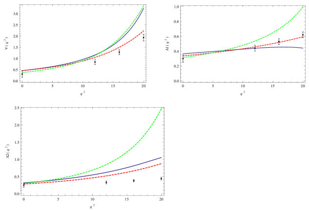
Figure 1: Comparison of the $B_{d}\to K^{\ast}$ transition form factors, Eqs. (33), (34) and (35) (black solid curve) with predictions from LQCD [10] (points with error bars), LCSR [4] (red dashed curve) and DSE [12] (green dashed curve).

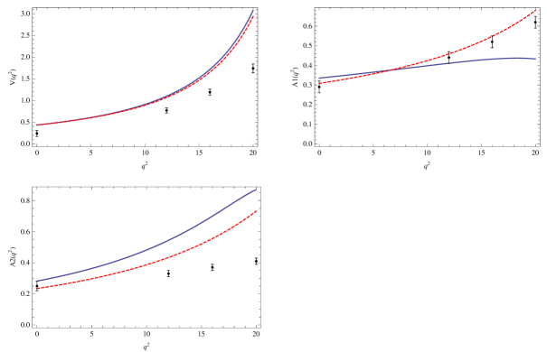
Figure 2: Comparison of form factors for $B_{s}\to\phi$; curve description as in Fig. 1 though no DSE results available in this transition.

The normalization of the form factors at $q^{2}=0$ can be expressed in terms of $g_{+}(q^{2}),g_{-}(q^{2})$, $h(q^{2})$ and $h_{1}(q^{2})$ which are discussed in detail in Refs. [13, 16]. Namely, we me make use of

$$\langle V(k,\varepsilon^{\ast})|\bar{s}i\sigma_{\alpha\beta}b|B(p)\rangle = -i\,\epsilon_{\alpha\beta\rho\sigma}\varepsilon^{\ast\rho}[(p+k)^{\sigma}g_{+}+q^{\sigma}g_{-}]-(\varepsilon^{\ast}\!\cdot q)\,\epsilon_{\alpha\beta\rho\sigma}(p+k)^{\rho}q^{\sigma}h$$ (19)

$$-i[(p+k)^{\alpha}\epsilon_{\beta\rho\sigma\tau}\varepsilon^{\ast\rho}(p+k)^{\sigma}q^{\tau}-\alpha\leftrightarrow\beta]\,h_{1}\ ,$$

so the form factors $V(q^{2}),A_{1,2}(q^{2}),F_{1,2,3}(q^{2})$ become,

$$F_{1}(q^{2}) = g_{+}(q^{2})-q^{2}h(q^{2})\ ,$$ (20)

$$F_{2}(q^{2}) = g_{+}(q^{2})+\frac{q^{2}}{M^{2}_{B}-M^{2}_{V}}\,g_{-}(q^{2})\ ,$$ (21)

$$F_{3}(q^{2}) = -g_{-}(q^{2})-(M^{2}_{B}-M^{2}_{V})h(q^{2})\ ,$$ (22)

and

$$V(q^{2}) = \frac{M_{B}+M_{V}}{m_{b}+m_{s}}\left[\,g_{+}(q^{2})-q^{2}h_{1}(q^{2})\right]\ ,$$ (23)

$$A_{1}(q^{2}) = \frac{M_{B}-M_{V}}{m_{b}-m_{s}}\left[g_{+}(q^{2})+\frac{q^{2}}{M^{2}_{B}-M^{2}_{V}}\,g_{-}(q^{2})\right]\ ,$$ (24)

$$A_{2}(q^{2}) = \frac{M_{B}-M_{V}}{m_{b}-m_{s}}\,\left[g_{+}(q^{2})-q^{2}h(q^{2})\right]-\frac{2M_{V}}{M_{B}-M_{V}}\,A_{0}(q^{2})\ .$$ (25)

At $q^{2}=0$, the form factors $F_{1}$, $F_{2}$, $V$ and $A_{1}$ in Eqs. (20), (21), (23) and (24) are thus parameterized by a single constant $g_{+}(0)$ whereas $A_{2}$ and $A_{0}$ in Eq. (25) can be expressed in terms of $g_{+}(0)$ and $A_{0}(0)$. It is well known that in case of real photon emission in $B_{d,s}\to V\gamma$ decays, the decay rate is a function of $g_{+}(0)$ [18]:

$$\Gamma(B\to V\gamma)=\frac{G_{F}^{2}\,\alpha_{\mathrm{em}}}{32\pi^{4}}|V_{tb}V_{ts}^{\ast}|^{2}m^{2}_{b}M^{3}_{B}\left(1-\tfrac{M^{2}_{V}}{M^{2}_{B}}\right)^{\!3}|C_{7}^{\mathrm{eff}}|^{2}|g_{+}(0)|^{2}.$$ (26)

Using the experimental values of branching ratios of $B_{d}\to K^{\ast}\gamma$ and $B_{s}\to\phi\gamma$ decays [9],

$$\mathrm{Br}(B_{d}\to K^{\ast}\gamma) = (4.33\pm 0.15)\times 10^{-5},$$ (27)

$$\mathrm{Br}(B_{s}\to\phi\gamma) = (3.6\pm 0.4)\times 10^{-5}\ ,$$ (28)

the extracted $g_{+}(0)$ for these decays are,

$$g_{+}(0)^{B_{d}\to K^{\ast}} = 0.365^{+0.025}_{-0.025},$$ (29)

$$g_{+}(0)^{B_{s}\to\phi} = 0.335^{+0.02}_{-0.02}\ .$$ (30)

With $g_{+}(0)$ in hand, the other unknown, i.e. $A_{0}(0)$, can be expressed in terms of it as [13],

$$A_{0}(0) = \left(\frac{1-M_{V}^{2}/M_{B}^{2}}{1+M_{V}^{2}/M_{B}^{2}}+\frac{M_{B}}{M_{V}}\right)g_{+}(0)\ .$$ (31)

It is worth mentioning that the form factor relations derived from Ward identities do not hold for the entire physical momentum, $q^{2}$, region. Therefore, we employ the following parametrization between $q^{2}=0$ and near the poles:

$$F(q^{2}) = \frac{F(0)}{(1-q^{2}/M^{2})(1-q^{2}/M^{\prime 2})}\ ,$$ (32)

where $M$ is $M_{B^{\ast}}(1^{-})$ or $M_{B^{\ast}_{A}}(1^{+})$ and $M^{\prime}$ is the radial excitation of $M$. The parametrization given in Eq. (32) not only takes into account the correction to the single pole dominance, as suggested by dispersion relations [26], but also help us to determine the couplings of $B^{\ast}$ or $B^{\ast}_{A}$ to the $BV$ channel [13, 14], which is not the aim of this work. Finally, using the above parameterization, the form factors can be expressed as:

$$V(q^{2}) = \frac{V(0)}{(1-q^{2}/M^{2}_{B^{\ast}})(1-q^{2}/M^{\prime 2}_{B^{\ast}})},$$ (33)

$$A_{1}(q^{2}) = \frac{A_{1}(0)}{(1-q^{2}/M^{2}_{B^{\ast}})(1-q^{2}/M^{\prime 2}_{B^{\ast}})}\left(1-\frac{q^{2}}{M^{2}_{B}-M^{2}_{V}}\right),$$ (34)

$$A_{2}(q^{2}) = \frac{{\tilde{A}_{2}}(0)}{(1-q^{2}/M^{2}_{B^{\ast}})(1-q^{2}/M^{\prime 2}_{B^{\ast}})}-\frac{2M_{V}}{M_{B}-M_{V}}\frac{A_{0}(0)}{(1-q^{2}/M^{2}_{B})(1-q^{2}/M^{\prime 2}_{B})},$$ (35)

where $\tilde{A}_{2}(0)$ is defined as [13]:

$$\tilde{A}_{2}(0) = \left(\frac{M_{B}-M_{V}}{m_{b}-m_{s}}\right)\,g_{+}(0)\ .$$ (36)

The transition form factors in Eqs. (33), (34) and (35) are plotted as a function of $q^{2}$ in Figs. 1 and 2 for $B_{d}\to K^{\ast}$ and $B_{s}\to\phi$, respectively, where we use the Particle Data Group values for the masses of $B$, $B^{*}$, $B_{A}^{*}$ and their excited states [9]. In the same figures, we also compare our form factors with those obtained in the Lattice QCD and LCSR approaches and in case of the $B_{d}\to K^{\ast}$ transition the DSE form factors [12] are also included. The trend of the $V(q^{2})$ evolution we obtain parallels that of the DSE form factor, whereas our $A_{1}(q^{2})$ and $A_{2}(q^{2})$ compare more favorably with the LCSR results, as becomes clear from Fig. 1. Similarly, for the $B_{s}\to\phi\mu^{+}\mu^{-}$ decay, our form factors are mostly in agreement with LCSR predictions except for larger momenta, $q^{2}\gtrsim 10$ GeV²; see Fig. 2. It is also apparent that lattice QCD simulations produce a softer slope of the $A_{1}(q^{2})$ and $V(q^{2})$ form factors than the other calculations. For reference, we also list the form factor values at $q^{2}=0$ and $q^{2}=q^{2}_{\mathrm{max}}$ as well as their ratios in Tables 1 and 2.

	$V$	$A_{1}$	$A_{2}$	$\frac{V(q^{2}_{\mathrm{max}})}{V(0)}$	$\frac{A_{1}(q^{2}_{\mathrm{max}})}{A_{1}(0)}$	$\frac{A_{2}(q^{2}_{\mathrm{max}})}{A_{2}(0)}$
Present Work	0.456 (2.858)	0.365  (0.4476)	0.316  (1.007)	6.267	1.226	3.186
LCSR	0.457  (2.064)	0.337  (0.577)	0.282 (0.830)	4.516	1.712	2.943
LQCD	0.30  (1.93)	0.30  (0.62)	0.25  (0.44)	6.433	2.06	1.76
DSE	0.37  (2.98)	0.29  (1.28)	0.30 (2.177)	8.054	4.431	7.256

Table 1: Variation of form factors for the transition $B_{d}\to K^{\ast}$ at $q^{2}=0$ and $q^{2}=q^{2}_{\mathrm{max}}$ in different approaches. The first value represents the form factors at $q^{2}=0$ whereas the value at maximum $q^{2}$ is in parentheses. The ratios of the form factors at $q^{2}_{\mathrm{max}}$ and $q^{2}=0$ are listed in the last three columns.

	$V$	$A_{1}$	$A_{2}$	$\frac{V(q^{2}_{\mathrm{max}})}{V(0)}$	$\frac{A_{1}(q^{2}_{\mathrm{max}})}{A_{1}(0)}$	$\frac{A_{2}(q^{2}_{max})}{A_{2}(0)}$
Present Work	0.433  (2.566)	0.335  (0.436)	0.282  (0.828)	5.926	1.301	2.936
LCSR	0.434  (2.455)	0.311 (0.637)	0.234  (0.676)	5.656	2.048	2.888
Lattice	0.24  (1.74)	0.29  (0.62)	0.25  (0.41)	7.25	2.137	1.64

Table 2: Variation of form factors for the transition $B_{s}\to\phi$ at $q^{2}=0$ and $q^{2}=q^{2}_{\mathrm{max}}$ in different approaches. Table entries are as in Table 1.

3 Applications of Transition Form Factors: Branching Fractions

To conclude, we present the calculated branching ratios of the $B\to K^{*}\mu^{+}\mu^{-}$ and $B_{s}\to\phi\mu^{+}\mu^{-}$ decays, where we remind that the transition form factors are the major hadronic input as well as source of uncertainties. Here we use the form factors introduced in Section 2.2 and extrapolated via Eqs. (33), (34) and (35) to compute the differential branching fractions and compare them to those obtained with form factors of the corresponding LCSR, Lattice QCD and DSE approaches.

The formula for the differential decay rate is given by,

$$\frac{d^{2}\Gamma(B\to V\ell^{+}\ell^{-})}{d\cos\theta\,dq^{2}} = \frac{1}{2M^{3}_{V}}\frac{2\beta\sqrt{\lambda}}{(8\pi)^{3}}|\,\mathcal{M}|^{2}$$ (37)

with $\mathcal{M}$ from Eq. (5) and where $\beta\equiv\sqrt{1-4m^{2}_{\ell}/s}$, $\lambda\equiv\lambda(M_{B},M_{V},s)=M^{4}_{B}+M^{4}_{V}+q^{4}-2M^{2}_{{B}}M^{2}_{V}-2q^{2}M^{2}_{B}-2q^{2}M^{2}_{V}$. The explicit form of differential decay rates for the decay $B_{d}\to K^{\ast}\mu^{+}\mu^{-}$ and $B_{s}\to\phi\mu^{+}\mu^{-}$ can be found in Ref. [27]. The plot of the differential branching fractions, $d\Gamma(B\to V\ell^{+}\ell^{-})/dq^{2}$, for the above mentioned decays in different approaches are depicted in Figs. 3a and 3b. The functional form of the differential branching fractions we obtain is comparable with the one using other form factor calculations, albeit with variations in magnitude. Note, however, that the DSE approach leads to a stronger variation of $d\Gamma/dq^{2}$ with $q^{2}$ in the $B\to K^{*}$ transition.

Furthermore, numerical values of branching ratios of $B_{d}\to K^{\ast}\mu^{+}\mu^{-}$ and $B_{s}\to\phi\mu^{+}\mu^{-}$ decays are listed in Table 3. The $B_{d}\to K^{\ast}\mu^{+}\mu^{-}$ branching ratio obtained with transition form factors of the DSE based model lies close to the experimental value. Within theoretical and experimental errors, both of which may be underestimated, our numerical results for both decays do agree with the PDG average. We cannot make a statement in case of the LQCD and LCSR results as no error estimate is given, yet the LQCD branching ratios are considerably larger than experimental values. This could be due to the fact that LQCD does not produce as strongly rising form factors, hence might not describe a VMD behavior. In the case of the $B_{s}\to\phi\mu^{+}\mu^{-}$ decay, the discrepancy between the experimental average and LCSR and LQCD values is equally large. It is worthwhile to remind that the values of $g_{+}(0)$, Eqs. (29) and (30), are very similar. Given that the functional form of the $V(q^{2})$, $A_{1}(q^{2})$ and $A_{2}(q^{2})$ form factors of the $B_{d}\to K^{\ast}$ transition is not noticeable different from the one in $B_{s}\to\phi$ and that the phase space difference is minor, we do not expect very different branching ratio values.

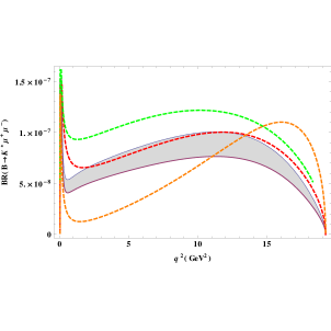
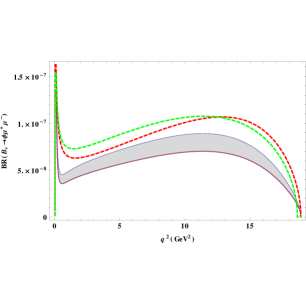
Figure 3: Differential branching fractions, $d\Gamma/dq^{2}$, for the decays $B_{d}\to K^{\ast}\mu^{+}\mu^{-}$ (left panel) and $B_{s}\to\phi\mu^{+}\mu^{-}$ (right panel). The gray-shaded band represents the estimated error of the differential branching fraction in the present approach; the same branching fractions computed with the LCSR, Lattice QCD and DSE form factors are plotted with red-dashed, green-dashed and orange-dashed curves, respectively.

	Br$(B_{d}\to K^{\ast}\mu^{+}\mu^{-})$	Br$(B_{s}\to\phi\mu^{+}\mu^{-})$
Present Work	$(1.37\pm 0.2)\times 10^{-6}$	$(1.21\pm 0.15)\times 10^{-6}$
LCSR	$1.31\times 10^{-6}$	$1.70\times 10^{-6}$
Lattice	$1.97\times 10^{-6}$	$1.67\times 10^{-6}$
DSE	$1.18\times 10^{-6}$	—
PDG	$(1.06\pm 0.09)\times 10^{-6}$	$(7.6\pm 1.5)\times 10^{-7}$

Table 3: Numerical values of branching ratios for the semileptonic decays $B_{d}\to K^{\ast}\mu^{+}\mu^{-}$ and $B_{s}\to\phi\mu^{+}\mu^{-}$ in different form factors approaches.

References

- [1] S. L. Glashow, J. Iliopoulos, and L. Maiani, Phys. Rev. D 2, 1285 (1970).
- [2] M. S. Alam et al. Phys. Rev. Lett. 74, 2885 (1995).
- [3] R. Ammar et al., Phys. Rev. Lett. 71, 674 (1993); CLEO CONF 96-05 (1996).
- [4] A. Ali, P. Ball, L. T. Handoko and G. Hiller, Phys. Rev. D 61, 074024 (2000).
- [5] T. M. Aliev, M. K. Cakmak and M. Savci, Nucl. Phys. B 607, 305 (2001); T. M. Aliev, A. Ozpineci, M. Savci and C. Yuce, Phys. Rev. D 66, 115006 (2002); T. M. Aliev, A. Ozpineci and M. Savci, Phys. Lett. B 511, 49 (2001); T. M. Aliev and M. Savci, Phys. Lett. B 481, 275 (2000); T. M. Aliev, D. A. Demir and M. Savci, Phys. Rev. D 62, 074016 (2000); T. M. Aliev, C. S. Kim and Y. G. Kim, Phys. Rev. D 62, 014026 (2000); T. M. Aliev and E. O. Iltan, Phys. Lett. B 451, 175 (1999); C. H. Chen and C. Q. Geng, Phys. Rev. D 66, 034006 (2002); C. H. Chen and C. Q. Geng, Phys. Rev. D 66, 014007 (2002); G. Erkol and G. Turan, Nucl. Phys. B 635, 286 (2002); E. O. Iltan, G. Turan and I. Turan, J. Phys. G 28, 307 (2002); T. M. Aliev, V. Bashiry and M. Savci, JHEP 0405, 037 (2004); W. J. Li, Y. B. Dai and C. S. Huang, Eur. Phys. J. C 40, 565 (2005); Q. S. Yan, C. S. Huang, W. Liao and S. H. Zhu, Phys. Rev. D 62, 094023 (2000); S. R. Choudhury, N. Gaur, A. S. Cornell and G. C. Joshi, Phys. Rev. D 68, 054016 (2003); S. R. Choudhury, A. S. Cornell, N. Gaur and G. C. Joshi, Phys. Rev. D 69, 054018 (2004).
- [6] A. Ali, E. Lunghi, C. Greub and G. Hiller, Phys. Rev. D 66, 034002 (2002); F. Kruger and E. Lunghi, Phys. Rev. D 63, 014013 (2001).
- [7] S. Rai Choudhury , N. Gaur and N. Mahajan, Phys. Rev. D 66, 054003 (2002); T. M. Aliev, V. Bashiry and M. Savci, Phys. Rev. D 71, 035013 (2005); U. O. Yilmaz, B. B. Sirvanli and G. Turan, Nucl. Phys. 692, 249 (2004); U. O. Yilmaz, B. B. Sirvanli and G. Turan, Eur. Phys. J. C 30, 197 (2003).
- [8] The LHCb Collaboration, R. Aaij et al. JHEP 08, 034 (2011); The LHCb Collaboration, R. Aaij et al. Preprint CERN-PH-EP-2011-106.
- [9] K. A. Olive et al. (Particle Data Group), Chin. Phys. C 38, 090001 (2014).
- [10] Ronald R. Horgan, Zhaofeng Liu, Stefan Meinel, Matthew Wingate, Phys. Rev. D 89, 094501 (2014).
- [11] P. Ball and R. Zwicky, Phys. Rev. D 71, 014029 (2005).
- [12] Mikhail A. Ivanov, Jürgen G. Körner, Sergey G. Kovalenko, and Craig D. Roberts Phys. Rev. D 76, 034018 (2007).
- [13] A. H. S. Gilani, Riazuddin and T. Al-Aithan, JHEP 0309, 065 (2003).
- [14] M. Saleh Khan, M. Jamil Aslam, A. H. S Gilani and Riazuddin, Eur. Phys. J.C 49, 665 (2007).
- [15] M. Ali Paracha, Ishtiaq Ahmed and M. Jamil Aslam, Eur. Phys. J.C 52, 967 (2007).
- [16] M. Ali Paracha, Ishtiaq Ahmed and M. Jamil Aslam, Phys. Rev. D 84, 035003 (2011).
- [17] J. Charles, A. Le Yaouanc, L. Oliver, O. Pène, J.-C. Raynal, Phys. Rev. D 60, 014001 (1999).
- [18] M. Jamil Aslam and Riazuddin, Phys. Rev. D 72, 094019 (2005); M. Jamil Aslam, Eur. Phys. J. C 49, 651 (2007).
- [19] A. J. Buras et al., Nucl. Phys. B 424, 374 (1994).
- [20] C.S. Kim, T. Morozumi, A.I. Sanda, Phys. Lett. B 218, 343 (1989); X. G. He, T. D. Nguyen and R. R. Volkas, Phys. Rev. D 38, 814 (1988); B. Grinstein, M. J. Savage, M. B. Wise, Nucl. Phys. B 319, 271 (1989); N. G. Deshpande, J. Trampetic and K. Panose, Phys. Rev. D 39, 1461 (1989); P. J. O’ Donnell and H. K. K. Tung, Phys. Rev. D 43, 2067 (1991); N. Paver and Riazuddin, Phys. Rev. D 45, 978 (1992); A. Ali, T. Mannel and T. Morozumi, Phys. Lett. B 273, 505 (1991); D. Melikhov, N. Nikitin and S. Simula, Phys. Lett. B 430, 332 (1998) [arXiv:hep-ph/9803343]; J. M. Soares, Nucl. Phys. B 367, 575 (1991); G. M. Asatrian and A. Ioannisian, Phys. Rev. D 54, 5642 (1996) [arXiv:hep-ph/9603318]; J. M. Soares, Phys. Rev. D 53, 24 (1996); C. H. Chen and C. Q. Geng, Phys. Rev. D 64, 074001(2001) [arXiv:hep-ph/0106193].
- [21] B. El-Bennich, M. A. Ivanov and C. D. Roberts, Nucl. Phys. Proc. Suppl. 199, 184 (2010).
- [22] B. El-Bennich, C. D. Roberts and M. A. Ivanov, arXiv:1202.0454 [nucl-th].
- [23] B. El-Bennich, G. Krein, L. Chang, C. D. Roberts and D. J. Wilson, Phys. Rev. D 85, 031502 (2012).
- [24] A. Bashir, L. Chang, I. C. Cloët, B. El-Bennich, Y. X. Liu, C. D. Roberts and P. C. Tandy, Commun. Theor. Phys. 58, 79 (2012).
- [25] E. Rojas, B. El-Bennich and J. P. B. C. de Melo, Phys. Rev. D 90, no. 7, 074025 (2014).
- [26] C. A. Dominguez, N. Paver and Riazuddin, Z. Physik C 48, 55 (1990).
- [27] Ishtiaq Ahmed, M. Jamil Aslam and M. Ali Paracha, Phys. Rev. D 89, 015006 (2014).