Semi-parametric modeling of excesses above high multivariate thresholds with censored data

Abstract.

How to include censored data in a statistical analysis is a recurrent issue in statistics. In multivariate extremes, the dependence structure of large observations can be characterized in terms of a non parametric angular measure, while marginal excesses above asymptotically large thresholds have a parametric distribution. In this work, a flexible semi-parametric Dirichlet mixture model for angular measures is adapted to the context of censored data and missing components. One major issue is to take into account censoring intervals overlapping the extremal threshold, without knowing whether the corresponding hidden data is actually extreme. Further, the censored likelihood needed for Bayesian inference has no analytic expression. The first issue is tackled using a Poisson process model for extremes, whereas a data augmentation scheme avoids multivariate integration of the Poisson process intensity over both the censored intervals and the failure region above threshold. The implemented MCMC algorithm allows simultaneous estimation of marginal and dependence parameters, so that all sources of uncertainty other than model bias are captured by posterior credible intervals. The method is illustrated on simulated and real data.

Keywords:  Multivariate extremes; censored data; data augmentation; semi-parametric Bayesian inference; MCMC algorithms.

1. Introduction

Data censoring is a commonly encountered problem in multivariate statistical analysis of extreme values. A ‘censored likelihood’ approach makes it possible to take into account partially extreme data (non concomitant extremes): coordinates that do not exceed some large fixed threshold are simply considered as left-censored. Thus, the possibly misleading information carried by non-extreme coordinates is ignored, only the fact that they are not extreme is considered (Smith, (1994); Ledford and Tawn, (1996); Smith et al., (1997), see also Thibaud and Opitz, (2013) or Huser et al., (2014)). However, there are other situations where the original data is incomplete. For example, one popular way to obtain large sample sizes in environmental sciences in general and in hydrology in particular, is to take into account data reconstructed from archives, which results in a certain amount of left- and right-censored data, and missing data. As an example, what originally motivated this work is a hydrological data set consisting of daily water discharge recorded at four neighboring stations in the region of the Gardons, in the south of France. The extent of systematic recent records is short (a few decades) and varies from one station to another, so that standard inference using only ‘clean’ data is unfeasible (only $3$ uncensored multivariate excesses of ‘large’ thresholds - fixed after preliminary uni-variate analysis- are recorded). Historical information is available, starting from the $17^{\text{th}}$ century, a large part of it being censored: only major floods are recorded, sometimes as an interval data (e.g. ‘the water level exceeded the parapet but the Mr. X’s house was spared’). These events are followed by long ‘blank’ periods during which the previous record was not exceeded. Uni-variate analysis for this data set has been carried on by Neppel et al., (2010) but a multivariate analysis of extremes has never been accomplished, largely due to the complexity of the data set, with multiple censoring.

While modeling multivariate extremes is a relatively well marked out path when ‘exact’ (non censored) data are at stake, many fewer options are currently available for the statistician working with censored data. The aim of the present paper is to provide a flexible framework allowing multivariate inference in this context. Here, the focus is on the methodology and the inferential framework is mainly tested on simulated data with a censoring pattern that resembles that of the real data. A detailed analysis of the hydrological data raises other issues, such as, among others, temporal dependence and added value of the most ancient data. These questions are addressed in a separate paper, intended for the hydrological community (Sabourin and Renard,, 2014).

Under a standard assumption of multivariate regular variation (see Section 2), the distribution of excesses above large thresholds is characterized by parametric marginal distributions and a non-parametric dependence structure that is independent from threshold. Since the family of admissible dependence structures is, by nature, too large to be fully described by any parametric model, non-parametric estimation has received a great deal of attention in the past few years (Einmahl et al.,, 2001; Einmahl and Segers,, 2009; Guillotte et al.,, 2011). To the best of my knowledge, the non parametric estimators of the so-called angular measure (which characterizes the dependence structure among extremes) are only defined with exact data and their adaptation to censored data is far from straightforward.

For applied purposes, it is common practice to use a parametric dependence model. A widely used one is the Logistic model and its asymmetric and nested extensions (Gumbel,, 1960; Coles and Tawn,, 1991; Stephenson,, 2009, 2003; Fougères et al.,, 2009). In the logistic family, censored versions of the likelihood are readily available, but parameters are subject to non linear constraints and structural modeling choices have to be made a priori, e.g., by allowing only bi-variate or tri-variate dependence between closest neighbors.

One semi-parametric compromise consists in using mixture models, built from a potentially infinite number of parametric components, such as the Dirichlet mixture model (DM), first introduced by Boldi and Davison, (2007). They have shown that it can approach arbitrarily well any valid angular measure for extremes. A re-parametrized version of the DM model (Sabourin and Naveau,, 2014), allows for consistent Bayesian inference - thus, a straightforward uncertainty assessment using posterior credible sets - with a varying number of mixture components via a reversible-jumps algorithm. The approach is appropriate for data sets of moderate dimension (typically, $d\approx 5$).

The purpose of the present work is to adapt the DM  model to the case of censored data. The difficulties are two-fold: First, from a modeling perspective, when the censoring intervals overlap the extremal thresholds (determined by preliminary analysis), one cannot tell whether the event must be treated as extreme. The proposed approach here consists in reformulating the Peaks-over-threshold (POT) model originally proposed by Boldi and Davison, (2007) and Sabourin and Naveau, (2014), in terms of a Poisson model, in which the censored regions overlapping the threshold have a well-defined likelihood. The second challenge is numerical and algorithmic: for right-censored data above the extremal threshold (not overlapping it), the likelihood expression involves integrals of a density over rectangular regions, which have no analytic expression. The latter issue is tackled within a data augmentation framework, which is implemented as an extension of Sabourin and Naveau, (2014)’s algorithm for Dirichlet mixtures.

An additional issue addressed in this paper concerns the separation between marginal parameters estimation and estimation of the dependence structure. Performing the two steps separately is a widely used approach, but it boils down to neglecting marginal uncertainty, which confuses uncertainty assessment about joint events such as probabilities of failure regions. It also goes against the principle of using regional information together with the dependence structure to improve marginal estimation, which is the main idea of the popular regional frequency analysis in hydrology. In this paper, simultaneous inference of marginal and dependence parameters in the DM model is performed, which amounts in practice to specifying additional steps for the marginal parameters in the MCMC sampler.

The rest of this paper is organized as follows: Section 2 recalls the necessary background for extreme values modeling. The main features of the Dirichlet mixture model are sketched. This POT model is then reformulated as a Poisson model, which addresses the issue of variable threshold induced by the fluctuating marginal parameters. Censoring is introduced in Section 3. In this context, the Poisson model has the additional advantage that censored data overlapping threshold have a well defined likelihood.The lack of analytic expression for the latter is addressed by a data augmentation scheme described in Section 4. The method is illustrated by a simulation study in Section 5: marginal performance in the DM model and in an independent one (without dependence structure) are compared, and the predictive performance of the joint model in terms of conditional probabilities of joint excesses is investigated. The model is also fitted to the hydrological data. Section 6 concludes. Most of the technicalities needed for practical implementation, such as computation of conditional distributions, or details concerning the data augmentation scheme and its consistency are relegated to the appendix.

2. Model for threshold excesses

2.1. Dependence structure model: angular measures

In this paper, the sample space is the $d$-dimensional Euclidean space $\mathbb{R}^{d}$, endowed with the Borel $\sigma$-field. In what follows, bold symbols denote vectors and, unless otherwise mentioned, binary operators applied to vectors are defined component-wise. Let $(\mathbf{Y}_{t})_{t\in\mathbb{N}}$ be independent, identically distributed (i.i.d.) random vectors in $\mathbb{R}^{d}$, with joint distribution $\mathbf{F}$ and margins $F_{j}$, $1\leq j\leq d$. The joint behavior of large observations is best expressed in terms of standardized data. Namely, define

$$\mathbf{X}_{t}=(-1/\log(F_{1}(Y_{1,t})),\dotsc,-1/\log(F_{d}(Y_{d,t})))\,.$$

Then the $X_{j,t}$’s have unit-Fréchet distribution, $\mathbb{P}(X_{j,t}\leq x)=e^{-1/x}$, $x>0$. It is mathematically convenient to switch to pseudo-polar coordinates,

$$R=\sum_{j=1}^{d}X_{j}\;(\text{\emph{radial component}}),\quad\mathbf{W}=\frac{1}{R}\mathbf{X}\in\mathbf{S}_{d}\;(\text{\emph{angular component}})\,,$$

where $\mathbf{S}_{d}=\{\mathbf{x}:x_{j}\geq 0,\sum_{j=1}^{d}x_{j}=1\}$ is the unit simplex. The radial variable $R$ corresponds to the ‘amplitude’ of the data whereas the angular component $\mathbf{W}$ characterizes their ‘direction’. Asymptotic theory (Resnick,, 1987; Beirlant et al.,, 2004; Coles,, 2001) tells us that, under mild assumptions on $\mathbf{F}$ (namely, belonging to a multivariate maximum domain of attraction), an appropriate model, commonly referred to as a multivariate Peaks-over-threshold (POT) model, for $(R,\mathbf{W})$ over high radial thresholds $r_{0}$, is

$$\mathbb{P}(R>r,\mathbf{W}\in A\;|\;R>r_{0})=\frac{r}{r_{0}}H(A)\;,\qquad r_{0}>r,A\subset\mathbf{S}_{d}\,,$$ (2.1)

where $H$ is the so-called ‘angular probability measure’ (called the ‘angular measure’ in the remainder of this paper). The angular measure is thus the limiting distribution of the angle, given that the radius is large. Concentration of $H$’s mass in the middle of the simplex indicates strong dependence at extreme levels, whereas Dirac masses only on the vertices characterizes asymptotic independence. This paper focuses on the case where $H$ is concentrated on the interior of the simplex, so that all the variables are asymptotically dependent.

Because of the standardization to unit Fréchet, a probability measure $H$ on $\mathbf{S}_{d}$ is a valid angular measure if and only if $\int_{\mathbf{S}_{d}}w_{j}\,\,\textup{d}H(\mathbf{w})=\frac{1}{d}\quad(1\leq j\leq d)\,.$ This moments constraint is the only condition on $H$, so that the angular measure has no reason to be part of any particular parametric family.

2.2. Dirichlet mixture angular measures

In this paper, the angular measure $H$ is modeled by a Dirichlet mixture distribution (Boldi and Davison,, 2007; Sabourin and Naveau,, 2014). A Dirichlet distribution can be characterized by a shape $\nu\in\mathbb{R}^{+}$ and a center of mass $\boldsymbol{\mu}\in\mathbf{S}_{d}$, so that its density with respect to the $d-1$ dimensional Lebesgue measure $\,\textup{d}\mathbf{w}=\,\textup{d}w_{1}\dotsb\,\textup{d}w_{d-1}$, is

$$\operatorname{diri}_{\nu,\boldsymbol{\mu}}(\mathbf{w})=\frac{\Gamma(\nu)}{\prod_{j=1}^{d}\Gamma(\nu\mu_{j})}\prod_{j=1}^{d}w_{j}^{\nu\mu_{j}-1}\,\qquad(\mathbf{w}\in\mathbf{S}_{d}).$$ (2.2)

A parameter for a $k$-mixture is of the form

$$\psi=\left((\mathit{p}_{1},\dotsc,\mathit{p}_{k}),(\boldsymbol{\mu}_{1},\dotsc,\boldsymbol{\mu}_{k}),(\nu_{1},\dotsc,\nu_{k})\right)\,,$$

with weights $\mathit{p}_{m}>0$, such that $\sum_{m=1}^{k}\mathit{p}_{m}=1$. This is summarized by writing $\psi=\left(\mathit{p}_{1:k},\boldsymbol{\mu}_{1:k},\nu_{1:k}\right)$. The corresponding mixture density is

$$h_{\psi}(\mathbf{w})=\sum_{m=1}^{k}\mathit{p}_{m}\operatorname{diri}_{\nu,\boldsymbol{\mu}_{m}}(\mathbf{w})\;.$$ (2.3)

the moments constraint is satisfied if and only if

$$\sum_{m=1}^{k}\mathit{p}_{m}\boldsymbol{\mu}_{m}=\left(1/d,\dotsc,1/d\right)\,,$$

which, in geometric terms, means that the center of mass of the $\boldsymbol{\mu}_{1:k}$’s, with weights $\mathit{p}_{1:k}$, must lie at the center of the simplex. As established by Boldi and Davison, (2007) and mentioned in the introduction, the family of Dirichlet mixture densities satisfying the moments constraint is weakly dense in the space of admissible angular measure. In addition, in a Bayesian framework, Sabourin and Naveau, (2014) have shown that the posterior is weakly consistent under mild conditions. These two features put together make the Dirichlet mixture model an adequate candidate for modeling the angular components of extremes.

2.3. Model for margins

The above model for excesses concerns standardized versions $\mathbf{X}_{t}$ of the data $\mathbf{Y}_{t}$ involving marginal cumulative distribution function $F_{j}$ ($1\leq j\leq d$), which have to be estimated. As a consequence of uni-variate extreme value theory (Pickands,, 1975), uni-variate excesses above large thresholds $v_{j}$ ($1\leq j\leq d$) are approximately distributed according to a Generalized Pareto distribution with parameters $\xi_{j}$ (shape) and $\sigma_{j}$ (scale parameter),

$$P(Y_{j}>y\;|\;Y_{j}>v_{j})\approx_{v_{j}\to\infty}(1+\xi_{j}\frac{y-v_{j}}{\sigma_{j}})^{-1/\xi_{j}}\,.$$

A widely used method to model the largest excesses is a follows: Define a high multivariate threshold $\mathbf{v}=(v_{1},\dotsc,v_{d})$ and call ‘marginal excess’ any $Y_{j,t}>v_{j}$. Then, marginal excesses above $v_{j}$ are modeled as generalized Pareto random variables with parameters $\xi_{j}$ and $\sigma_{j}$. The marginal parameters are gathered into a $(2d)$-dimensional vector

$$\chi=\left(\log(\sigma_{1}),\dotsc,\log(\sigma_{d}),\xi_{1},\dotsc,\xi_{d}\right)\in\mathbb{R}^{2d}.$$

Let $F_{j}^{\mathbf{v}}$ denote the $j^{th}$ marginal distribution conditionally on $Y_{j}$ not exceeding $v_{j}$, and let $\zeta_{j}=\mathbf{P}(Y_{j}>v_{j})$ denote the probability of excursion above $v_{j}$. The $j^{th}$ marginal model ($1\leq j\leq d$) is thus

$$F_{j}^{(\chi)}(y) =\mathbf{P}(Y_{j,t}\leq y\,|\,\xi_{j},\sigma_{j})$$ (2.4)

$$=\begin{cases}1-\zeta_{j}\left(1+\xi_{j}\frac{y-v_{j}}{\sigma_{j}}\right)^{-1/\xi_{j}}&(y\geq v_{j}),\\ (1-\zeta_{j})F_{j}^{\mathbf{v}}(y)&(y<v_{j}).\end{cases}$$

It is common practice (Coles and Tawn,, 1991; Davison and Smith,, 1990) to use an empirical estimate $\hat{\boldsymbol{\zeta}}=(\hat{\zeta}_{1},\dotsc,\hat{\zeta}_{d})$ for the vector of probabilities of marginal excursion, and to ignore any estimation error, so that $\hat{\boldsymbol{\zeta}}$ is identified to $\boldsymbol{\zeta}$ is the sequel.

2.4. Joint inference in a Poisson model

When it comes to simultaneous estimation of the margins and of the angular measure, the angular model (2.1) for radial excesses is difficult to handle, because a radial failure region $r>r_{0}$ on the Fréchet scale (i.e.  , in terms of $\mathbf{X}$’s) corresponds to a complicated shaped failure region on the original scale, which depends on the marginal parameters and, accordingly, potentially contains a varying number of data points. It seems more reasonable to use a failure region which is fixed on the original scale (in terms of $\mathbf{Y}$’s). Further, a common criticism towards radial failure regions (Ledford and Tawn,, 1996) is that the marginal Pareto model is not valid near the axes of the positive orthant. Last but not least, censoring occurs along the directions of the Cartesian coordinate system, which prevents using the polar model (2.1) as it is. To address these issues, the statistical model for threshold excesses developed in this paper uses a ‘rectangular’ threshold. Also, it will be very convenient (see Section 3.3) to adopt a Poisson process representation of extremes (see e.g. Coles and Tawn,, 1991) as an alternative to the POT model (2.1), with a ‘censored likelihood’ near the axes.

Poisson model

Under the same condition of domain of attraction as above, the point process formed by time-marked, standardized and suitable re-scaled data converges in distribution to a Poisson process (see e.g. Resnick,, 1987, 2007; Coles and Tawn,, 1991),

$$\sum_{t=1}^{n}\mathds{1}_{(\frac{t}{n},\frac{\mathbf{X}_{t}}{n})}\overset{w}{\longrightarrow}\operatorname{PP}(\ell\otimes\lambda)\,,$$ (2.5)

in the space of point measures on $([0,1]\times\mathbf{E})$, where $\mathbf{E}=[0,\infty]^{d}\setminus\{0\}$. The temporal component $\ell$ of the limiting intensity measure denotes the Lebesgue measure on $\mathbb{R}$ and $\lambda$, the so-called exponent measure, is homogeneous of order $-1$, and is related to the angular measure $H$ via

$$\,\textup{d}\lambda(r,\mathbf{w})=\frac{d}{r^{2}}\;\,\textup{d}r\,\textup{d}H(\mathbf{w})\,.$$ (2.6)

From a statistical perspective, consider a failure region $A_{\mathbf{v}}=\mathbf{E}\setminus[\mathbf{0},\mathbf{v}]$, where $\mathbf{v}$ is the high multivariate threshold introduced in section 2.3 and $[\mathbf{0},\mathbf{v}]=[0,v_{1}]\times\dotsb\times[0,v_{d}]\setminus\{\mathbf{0}\}$. Call ‘excess above $\mathbf{v}$’ any point $\mathbf{Y}_{t}$ in $A_{\mathbf{v}}$, as opposed to marginal excesses $Y_{j,t}>v_{j}$. The Fréchet re-scaled multivariate threshold is

$$\boldsymbol{u}=\mathbf{T}(\mathbf{v})=-1/\log(1-\boldsymbol{\zeta})$$

and does not depend on $\chi$. Consider the re-scaled region on the Fréchet scale

$$A_{\boldsymbol{u},n}=\frac{1}{n}\mathbf{T}(A_{\mathbf{v}})=[0,\infty]^{d}\setminus[0,\frac{u_{1}}{n}]\times\dotsb\times[0,\frac{u_{d}}{n}]\,,$$

and denote $A_{\boldsymbol{u}}=A_{\boldsymbol{u},1}$. Applying the marginal transformations

$$\mathcal{T}_{j}^{\chi}(y)=-1/\log\left(F_{j}^{(\chi)}(y)\right)\,,$$

the marginal variables $X_{j,t}=\mathcal{T}_{j}^{\chi}(Y_{j,t})$ have unit Fréchet distribution, as required in (2.5). The point process $\mathbf{N}=\sum_{t=1}^{n}\mathds{1}_{(\frac{t}{n},\frac{\mathbf{X}_{t}}{n})}$ composed of the excesses $\mathbf{X}_{t}\in A_{\boldsymbol{u}}$ (i.e. $\mathbf{Y}_{t}\in A_{\boldsymbol{u}}$) is modeled according to the limit in (2.5),

$$\sum_{t=1}^{n}\mathds{1}_{(\frac{t}{n},\frac{\mathbf{X}_{t}}{n})}\sim\operatorname{PP}(\ell\otimes\lambda)\text{ on }[0,1]\times A_{\boldsymbol{u},n}\,,$$

where $\lambda$ is of the form (2.6), with angular component $H$ written as a Dirichlet mixture of the form (2.3).

Joint likelihood of uncensored data

Let $\theta=\left(\chi,\psi\right)$ be the parameter for the joint model. As explained at the beginning of this section, the model likelihood needs to be expressed in Cartesian coordinates. The density of an exponent measure $\lambda$ with respect to the $d$- dimensional Lebesgue measure $\,\textup{d}\mathbf{x}=\,\textup{d}x_{1}\dotsb\,\textup{d}x_{d}$, is (Coles and Tawn,, 1991, Theorem 1)

$$\frac{\,\textup{d}\lambda}{\,\textup{d}\mathbf{x}}(\mathbf{x})=d\,.\,r^{-(d+1)}h(\mathbf{w})\,.$$ (2.7)

Denote by $\lambda_{\psi}$ the exponent measure corresponding to the Dirichlet mixture $h_{\psi}$. Then, in the simplified case where the $\mathbf{Y}_{j,t}$’s are exactly observed and where the marginals $F_{j}$’s below threshold are known, the likelihood in the Poisson model over $A_{\mathbf{v}}$ is

$$\mathcal{L}_{\mathbf{v}}\left(\{\mathbf{y}_{t}\}_{1\leq t\leq n},\theta\right) \propto e^{-n\,\lambda_{\psi}(A_{\boldsymbol{u}})}\prod_{i=1}^{n_{\mathbf{v}}}\Big{\{}\frac{\,\textup{d}\lambda_{\psi}}{\,\textup{d}\mathbf{x}}(\mathbf{x}_{t_{i}})\prod_{j:y_{j,t_{i}}>v_{j}}J_{j}^{\chi}(y_{j,t_{i}})\Big{\}}\,,$$ (2.8)

where $t_{1},\dotsc,t_{n_{\mathbf{v}}}$ are the occurrence times of excesses $\mathbf{y}_{t_{i}}\in A_{\mathbf{v}}$, $x_{j,t_{i}}~{}=~{}T_{j}^{\chi}(y_{j,t_{i}})$, and the $J_{j}^{\chi}$ are Jacobian terms resulting from marginal transformations $T_{j}^{\chi}$ (see Appendix A for details).

3. Censored model

3.1. Causes of censoring

The presence of censored observations is the result of two distinct causes: first, data are partially observed, which results in interval- or right-censoring, which we call natural censoring. In addition, observed data points that exceed at least one threshold in one direction do not necessarily exceed all thresholds, so that the marginal extreme value model does not apply. Following Ledford and Tawn, (1996), those components are also considered as left-censored. This second censoring process is thus a consequence of an inferential framework which is designed for analyzing extreme values only, and we call it inferential censoring.

The total censoring process $\mathscr{C}$, which results from the juxtaposition of natural and inferential censoring, is assumed to be non informative. This means that (see also Gómez et al.,, 2004), if $F$ is the marginal c.d.f. for $Y_{j}$ and $f$ is the marginal density, then $Y_{j}$’s distribution conditional upon having observed only the left and right censoring bounds $(L,R)$ is $f(\,\cdot\,)/[F(R)-F(L)]$. This definition is easily extended to the multivariate case by replacing $F(R)-F(L)$ by the integral of the density over the censored directions (see e.g. Schnedler,, 2005, for a proof of consistency of maximum censored likelihood estimators).

3.2. Natural censoring

Call ‘Natural censoring’ the one which occurs independently from the choice of an extreme threshold $\mathbf{v}$ by the statistician. The observed process is denoted ${\mathbf{O}}=({\mathbf{O}}_{t})_{t}$, with $\mathbf{O}_{t}=(O_{1,t},\dotsc,O_{d,t})$. One marginal observation $O_{j,t}$ consists in a label $\kappa_{j,t}$ indicating presence or absence of censoring, together with the exact data $Y_{j,t}$ (if observed) or the censoring bounds $(L_{j,t},R_{j,t})$ (where $L_{j,t}$ may be set to $0$ in the case of left-censoring or missing data and $L_{j,t}=+\infty$ in the case of right-censored or missing data). In the sequel, $\kappa_{j,t}=0$ (resp. $1,2,3$) refer respectively to missing, exact, right- and left- censored data.

In this context, the ‘position’ of a marginal data $O_{j,t}$ with respect to the threshold is not necessarily well defined for censored data. Recall that we consider a case where the process of interest $(\mathbf{Y}_{t})_{t\geq 0}$ is stationary, whereas the censoring bounds vary with time, as a result of external factors on the observation process. When the censoring interval overlaps the threshold, i.e. , $v_{j}\in(L_{j,t},R_{j,t}),\kappa_{j}\in\{2,3\}$), the statistician does not know if an excess occurred or not. This situation is described here as $O_{j,t}$ marginally overlapping the threshold. The different positions of $O_{j,t}$ with respect to $v_{j}$ encountered in the data set of interest in this paper are summarized in Figure 1.

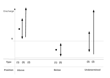
Figure 1. Position of marginal data points with respect to a marginal threshold $v$ (horizontal line). Black dots: marginal data points of type $\kappa=1$; vertical arrows: data of type $\kappa\in\{2,3\}$.

For a multivariate observation $\mathbf{O}_{t}$, if at least one coordinate marginally overlaps the threshold or is missing, and if the others are below the threshold, then the position of $\mathbf{O}_{t}$ with respect to the multivariate threshold $\mathbf{v}$ is undetermined. Indeed, $\mathbf{O}_{t}$ is below threshold if all its marginals are below the corresponding marginal threshold, and above threshold (in the failure region) otherwise. In the undetermined case, $\mathbf{O}_{t}$ is qualified as globally overlapping the threshold.

3.3. Inferential censoring below threshold

Since the marginal distributions $F_{j}^{\mathbf{v}}$’s, conditional upon not exceeding $v_{j}$, are unknown, the $X_{j,t}$’s such that $Y_{j,t}<v_{j}$ are not available. Instead of attempting to estimate the $F_{j}^{\mathbf{v}}$’s, one option is to censor the Fréchet-transformed components below threshold. More precisely, for a raw observation $O_{j,t}=(\kappa_{j,t},Y_{j,t},L_{j,t},R_{j,t})$, let us denote by $C_{j,t}^{\chi}=(\tilde{\kappa}_{j,t},X_{j,t},\tilde{L}_{j,t},\tilde{R}_{j,t})$ the corresponding ‘Fréchet transformed’ and censored one, and $\mathbf{C}_{t}^{\chi}$ the multivariate observation $(C_{1,t}^{\chi},\dotsc,C_{d,t}^{\chi})$. The transformation $\mathbf{O}_{t}\mapsto\mathbf{C}_{t}^{\chi}$ is illustrated in Figure 2 in the bi-variate case.

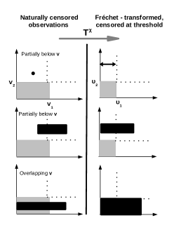
Figure 2. Example in the two-dimensional case of marginal transformation and censoring below threshold, for data of marginal types $(1,1)$, (upper panel) $(3,1)$ (middle panel) and $(3,3)$ (lower panel). In these three cases, observations are represented in black, respectively by a dot, an horizontal arrow and a rectangle. The Grey areas represent respectively the multivariate threshold $\mathbf{v}$ (left side) and the Fréchet transformed one $\boldsymbol{u}$ (right side). The two upper panels correspond to observations above threshold, while the lower panel shows an undetermined observation.

In a nutshell, inferential censoring occurs when the censoring intervals are below threshold or marginally overlapping it, or when an exact data component $Y_{j,t}<v_{j}$ is recorded. A formal definition of $C_{j}^{\chi}$ is as follows:

• $(\tilde{\kappa}_{j,t},X_{j,t})=\begin{cases}(3,\texttt{NA})&\text{if }\kappa_{j,t}=1\text{ and }Y_{j,t}<v_{j}\,,\\ (0,\texttt{NA})&\text{if }\kappa_{j,t}=2\text{ and }L_{j,t}<v_{j}\,,\\ \big{(}\kappa_{j,t},\mathcal{T}_{j}^{\chi}(Y_{j,t})\big{)}&\text{otherwise}.\end{cases}$

• $\tilde{L}_{j,t}=\begin{cases}0&\text{if }L_{j,t}<v_{j}\,,\\ \mathcal{T}_{j}^{\chi}(L_{j,t})&\text{otherwise. }\end{cases}$

• $\tilde{R}_{j,t}=\begin{cases}u_{j}&\text{if }R_{j,t}<v_{j}\,,\\ \mathcal{T}_{j}^{\chi}(R_{j,t})&\text{otherwise.}\end{cases}$

In the above definition, NA stands for a missing value and it is understood that $\mathcal{T}_{j}^{\chi}(\texttt{NA})=\texttt{NA}$.

In the end, observations globally overlapping threshold have their marginal lower bounds $\tilde{L}_{j,t}$ set to zero if $L_{j,t}<v_{j}$. The interest of using a Poisson model becomes clear at this point. Indeed, censored observations $\mathbf{C}_{t}^{\chi}$ obtained from observations $\mathbf{O}_{t}$ globally overlapping threshold correspond to events of the kind ‘The observation at time $t$ belongs to $\mathbf{[0},\mathbf{\tilde{R}}_{t}\mathbf{]}$’, which, by contrapositive, means ‘No point is observed outside of $\mathbf{[0},\mathbf{\tilde{R}}_{t}\mathbf{]}$ between $t$ and $t+1$’. This is written in terms of the Poisson process $\mathbf{N}$ as

$$\mathbf{N}\left(\left[\frac{t}{n},\frac{t+1}{n}\right)\times\left[\mathbf{0},\frac{\mathbf{\tilde{R}}_{t}}{n}\right]^{c}\right)=0\,,$$ (3.1)

which is a measurable event with respect to $\mathbf{N}$. The overlapping observations thus have a well defined likelihood in a Poisson model, as detailed in the next section, whereas they could not be taken into account in Sabourin and Naveau, (2014)’s POT model.

3.4. Poisson likelihood with censored and missing data

Due to the combination of natural and inferential censoring, the data set (from which missing days are excluded) is decomposed into data in the failure region, data overlapping threshold and data below threshold. Let $n_{\mathbf{v}}$, $n_{\mathbf{v}}^{\prime}$ and $n_{\mathbf{v}}^{\prime\prime}$ be the respective number of observations in each category. The number of non missing days is thus

$$n_{\text{obs}}=n_{\mathbf{v}}+n^{\prime}_{\mathbf{v}}+n^{\prime\prime}_{\mathbf{v}}\,,$$

and the number of ‘determined’ data (i.e. not overlapping $\mathbf{v}$) is

$$n_{\text{det}}=n_{\mathbf{v}}+n^{\prime\prime}_{\mathbf{v}}\,.$$

The $n_{\mathbf{v}}$ Fréchet-transformed observations $\{\mathbf{C}_{t_{i}}^{\chi}\}(i\in\{1,\dotsc,n_{\mathbf{v}}\})$ correspond to events of the kind

$$\mathbf{X}_{t_{i}}\in\mathbf{[}\mathbf{\tilde{L}}_{t_{i}}\boldsymbol{,\tilde{R}}_{t_{i}}\mathbf{]}\qquad\text{(rectangular region)}$$

where $\tilde{R}_{j,t_{i}}=\tilde{L}_{j,t_{i}}=X_{j,t_{i}}$ in the case of exact data.

Observations overlapping threshold correspond to events of the kind (3.1) introduced in the previous section. When a limited number $\mathcal{I}^{\prime}$ of right censoring bounds $\mathbf{R}_{t}=(R_{1,t},\dotsc,R_{d,t})$ are present, it is convenient to classify these overlapping events accordingly, writing $n^{\prime}_{\mathbf{v}}=\sum_{i=1}^{\mathcal{I}^{\prime}}n^{\prime}_{i}$ where $n^{\prime}_{i}$ is the number of observations with right censoring bound $\mathbf{R}_{t_{i}}$. Since the Poisson process is temporally exchangeable, there is no loss of generality in assuming that the latter observations occur at consecutive dates $(t^{\prime}_{i},\dotsc,t^{\prime}_{i}+n^{\prime}_{i}-1)$. The region $\mathbf{E}\setminus[\mathbf{0},\mathbf{\tilde{R}}_{t^{\prime}_{i}}]$ is ‘missed’ by the Fréchet re-scaled process $\mathbf{X}_{t}$ during this time period.

With theses notations, the censored likelihood in the Poisson model may be written

$$\mathcal{L}_{\mathbf{v}}(\mathbf{O},\theta) =\exp\Big{[}-n_{\text{det}}\,\lambda_{\psi}(A_{\boldsymbol{u}})-\sum_{i=1}^{\mathcal{I}^{\prime}}n^{\prime}_{i}\lambda_{\psi}(A^{\prime}_{i})\Big{]}\times\dotsb$$ (3.2)

$$\dotsb\,\prod_{i=1}^{n_{\mathbf{v}}}\Big{\{}\int_{\mathbf{[}\mathbf{\tilde{L}}_{t_{i}}\boldsymbol{,\tilde{R}}_{t_{i}}\mathbf{]}}\frac{\,\textup{d}\lambda_{\psi}}{\,\textup{d}\mathbf{x}}\,\textup{d}\ell_{i}(\mathbf{x})\prod_{j:y_{j,t_{i}}>v_{j}}J_{j}^{\chi}(y_{j,t_{i}})\Big{\}}\,,$$

where notation ‘$\,\textup{d}\ell_{i}(\mathbf{x})$’ in the integral terms is a shorthand for ‘the Lebesgue measure of dimension equal to that of $\mathbf{[}\mathbf{\tilde{L}}_{t_{i}}\mathbf{,\tilde{R}}_{t_{i}}\mathbf{]}$’ when the latter is greater than one, or ‘the Dirac mass at $\mathbf{x}_{t_{i}}=\mathbf{\tilde{L}}_{t_{i}}=\mathbf{\tilde{R}}_{t_{i}}$’ for exact data. Compared with the uncensored likelihood (2.8), $n$ has been replaced with $n_{\text{obs}}$, the exponential term for the non overlapping data follows from

$$\exp\Big{(}-\frac{n_{\text{det}}}{n_{\text{obs}}}\lambda_{\psi}\big{(}A_{\boldsymbol{u},n_{\text{obs}}}\big{)}\Big{)}=\exp\Big{(}-n_{\text{det}}\,\lambda_{\psi}\big{(}A_{\boldsymbol{u}}\big{)}\Big{)}\,,$$

and a similar argument yields the additional terms $\exp(-n^{\prime}_{i}\lambda_{\psi}(A^{\prime}_{i}))$ for overlapping data.

At this stage, the model has been entirely specified. The remaining issue concerns the treatment of the integral terms

$$\int_{\mathbf{[}\mathbf{\tilde{L}}_{t_{i}}\mathbf{,\tilde{R}}_{t_{i}}\mathbf{]}}\frac{\,\textup{d}\lambda_{\psi}}{\,\textup{d}\mathbf{x}}\,\textup{d}\ell_{i}(\mathbf{x})$$ (3.3)

and the exponential terms

$$\exp\Big{[}-n_{\text{det}}\,\lambda_{\psi}(A_{\boldsymbol{u}})\big{]}\qquad\text{and}\qquad\exp\Big{[}-n^{\prime}_{i}\lambda_{\psi}(A^{\prime}_{i})\Big{]}\,,$$ (3.4)

which have no analytic expression, as they require integrating $\lambda_{\psi}$ over rectangular regions. First, the dimension of numerical integration can be reduced as far as ‘missing coordinates’ are involved, because partial integration of $\lambda_{\psi}$ over $[0,\infty]$ in one direction has an exact expression. The model is stable under marginalization, in the sense that the obtained marginal exponent measures correspond again to Dirichlet mixtures on a lower dimensional simplex (see Appendix B for details). However, no closed form is available for the integral in the remaining censored directions, nor for the exponent measures of $A_{\boldsymbol{u}}$ or the $A^{\prime}_{i}$’s. This problem is tackled in the next section via a data augmentation method.

4. Data augmentation

4.1. Background

In a Bayesian context, one major objective is to generate parameter samples approximately distributed according to the posterior. In classical MCMC algorithms, the value of the likelihood is needed to define the transition kernel. Evaluating the integrated likelihood $\mathcal{L}_{\mathbf{v}}(\mathbf{O},\theta)$ at each iteration of the algorithm seems unmanageable: The dimension of integration can grow up to $d$, for each observation, and the shape of the integrand varies from one iteration to another, which is not favorable to standard quadrature methods. In particular, large or low values of the shape parameters $\nu_{m}$ in $\psi$ induce concentration of the integrand around the centers $\boldsymbol{\mu}_{m}$ or unboundedness at the simplex boundaries. Instead, data augmentation methods (see e.g. Tanner and Wong,, 1987; Van Dyk and Meng,, 2001) treat missing or partially observed data as additional parameters, so that the numerical integration step is traded against an increased dimension of the parameter space. In this section, $[\,\cdot\,]$ denotes the distribution of a random quantity as well as its density with respect to some appropriate reference measure. Proportionality between $\sigma$-finite measures is denoted by $\propto$. Thus, $[\theta]$ is the prior density and $[\theta\,|\,\mathbf{O}]\propto[\theta]\,\mathcal{L}_{\mathbf{v}}(\mathbf{O},\theta)$ is the posterior.

The main idea is to define an augmentation space $\mathcal{Z}$, and a probability measure $[\,\cdot\,|\mathbf{O}]_{+}$, on the augmented space $\Theta\times\mathcal{Z}$, conditional on the observations, which may be sampled using classical MCMC methods, and which is consistent with the ‘objective distribution’ on $\Theta$. That is, the posterior on $\Theta$ must be obtained by marginalization of $[\,\cdot\,|\,\mathbf{O}]_{+}$,

$$[\theta|\mathbf{O}]=\int_{\mathcal{Z}}[z,\theta\,|\,\mathbf{O}]_{+}\,\textup{d}z\,.$$ (4.1)

In the sequel, the invariant measure (or its density) $[z,\theta\,|\,\mathbf{O}\,]_{+}$ is referred to as the augmented posterior.

4.2. Data augmentation in the Poisson model

In our context, finding an augmentation random variable $Z_{+}$ with easily manageable conditional distributions, such that the augmented posterior $[z,\theta|\,\mathbf{O}]_{+}$ satisfy (4.1), is far from straightforward, mainly due to the exponential terms (3.4) in the likelihood.

Instead, an intermediate variable $\mathbf{Z}$ is introduced, which plays the role of a proposal distribution in the MCMC algorithm. $\mathbf{Z}$ is defined conditionally to $\theta$, through the augmented likelihood $[\,\mathbf{z},\mathbf{O}\,|\,\theta\,],$ so that the full conditionals $[\mathbf{Z}\;|\;\theta,\mathbf{O}]$ can be directly simulated as block proposals in a Metropolis-within-Gibbs algorithm (Tierney,, 1994). To ensure the marginalization condition (4.1), the augmented posterior $[\mathbf{Z},\theta|\,\mathbf{O}]_{+}$ is not the same as $[\mathbf{Z},\theta|\,\mathbf{O}]$. Instead it has a density of the form

$$[\mathbf{z},\theta\;|\;\mathbf{O}]_{+}\;\propto\;[\mathbf{z},\mathbf{O}\;|\;\theta\,]\;[\,\theta\,]\;\varphi(\mathbf{z})\,,$$ (4.2)

where $\varphi(\mathbf{z})$ is any weight function allowing to enforce the consistency condition (4.1). The $[\theta]$ terms cancel out and the latter condition is equivalent to

$$\mathcal{L}_{\mathbf{v}}(\mathbf{O},\theta)\propto\int[\mathbf{z},\mathbf{O}\;|\;\theta]\;\varphi(\mathbf{z})\,\textup{d}\mathbf{z}\,.$$ (4.3)

In the end, a posterior sample from $[\theta|\mathbf{O}]$ is simply obtained by ignoring the $\mathbf{Z}$-components from the one produced with the ‘augmented’ Markov chain.

In our case, the augmented data $\mathbf{Z}$ consist of two parts, $\mathbf{Z}=(\mathbf{Z}_{\text{above}},\mathbf{Z}^{\prime})$. The first one, $\mathbf{Z}_{\text{above}}=\{\mathbf{Z}_{t_{i}}\}_{i\leq n_{\mathbf{v}}}$, accounts for integral terms (3.3), while the second one, $\mathbf{Z}^{\prime}=(\mathbf{Z}^{\prime}_{\boldsymbol{u}},\{\mathbf{Z}^{\prime}_{i}\}_{i\leq\mathcal{I}^{\prime}})$, accounts for the exponential terms (3.4). The $\mathbf{Z}_{t_{i}}$’s have an intuitive interpretation, which is standard in data augmenting methods: they replace the censored $X_{j,t_{i}}$’s. On the contrary, the $\mathbf{Z}^{\prime}_{i}$’s and the $\mathbf{Z}^{\prime}_{\boldsymbol{u}}$ are just a computational trick accounting for the exponential terms: they are the points of independent Poisson processes defined on ‘nice’ radial sets containing the failure regions of interest $A^{\prime}_{i}$’s and $A_{\boldsymbol{u}}$, and $\varphi$ is a smoothed version of an indicator function of the failure regions.

The augmented likelihood factorizes as

$$[\;\mathbf{z},\mathbf{O}\;|\;\theta\;]=\prod_{i=1}^{n_{\mathbf{v}}}\big{\{}[\,\mathbf{z}_{t_{i}},\mathbf{O}_{t_{i}}\;|\;\theta\,]\big{\}}\,[\,\mathbf{z}^{\prime}_{\boldsymbol{u}}\;|\;\psi]\,\prod_{i=1}^{\mathcal{I}^{\prime}}[\mathbf{z}^{\prime}_{i}\,|\,\psi]\,,$$ (4.4)

and the weight function $\varphi$ is of the form

$$\varphi(\mathbf{z})=\varphi_{{\boldsymbol{u}}}(\mathbf{z}^{\prime}_{\boldsymbol{u}})\prod_{i=1}^{\mathcal{I}^{\prime}}\varphi^{\prime}_{{i}}(\mathbf{z}^{\prime}_{i})\,.$$

A precise definition of $\mathbf{Z}_{\text{above}}$ is given in Appendix C.1, together with the expression of the corresponding contributions to the augmented likelihood, $[\,\mathbf{z}_{t_{i}}\,\mathbf{O}_{t_{i}}\,|\theta\,]$ . The full conditionals $[\mathbf{Z}_{\text{above}}\,|\mathbf{O}\,,\theta\,]$ are derived in C.2. The augmentation Poisson processes $\mathbf{Z}^{\prime}$, together with the weight $\varphi$ are defined in Appendix C.3, and the compatibility condition (4.3) is proved to hold in Appendix C.4.

4.3. Implementation of a MCMC algorithm on the augmented space

This section describes only the main features of the algorithm, more details are provided in Appendix D. The present algorithm is an extension of Sabourin and Naveau, (2014)’s one, who proposed a Metropolis-within-Gibbs algorithm to sample the posterior distribution of the angular measure in a POT framework (2.1), within the Dirichlet mixture model (2.3). The number of components in the Dirichlet mixture is not fixed in their model, and the MCMC allows reversible-jumps between parameters sub-spaces of fixed dimension, each corresponding to a fixed number of components in the Dirichlet mixture. Their algorithm approximates the posterior distribution $[\psi|\mathcal{W}]$, where $\psi$ is the DM parameter and $\mathcal{W}$ is an angular data set consisting of the angular components $W_{t}$ of data $X_{t}$ that have been normalized to Fréchet margins in a preliminary step.

In contrast, the present algorithm handles ‘raw’ data (not standardized to Fréchet margins), with censoring of various types as described in Section 3, so as to approach the full posterior distribution (marginal and dependence parameters) $[\,\theta\;|\;\mathbf{O}\,]$ . In practice, this amounts to allowing two additional move types in the Metropolis-within-Gibbs sampler: marginal moves (updating the marginal parameters) and augmentation moves updating the augmentation data $\mathbf{Z}$ described above. The reversible jumps and the moves updating the DM parameters keeping the dimension constant are unchanged.

5. Simulations and real case example

Keeping in mind the application, the aim of this section is to verify that the algorithm provides reasonable estimates with data sets that ‘resemble’ the particular one motivating this work.

After a description of the experimental setting, an example of results obtained with a single random data set is given, then a more systematic study is conducted over 50 independent data sets. Finally, a brief description of the results obtained with the original hydrological data is provided. The latter part is kept short because, as mentioned in introduction, from a hydrological point of view, a full discussion of the benefits brought by historical information, as well as treatment of temporal dependence in the case of heavily censored data is needed and will be the subject of a separate paper.

5.1. Experimental setting

For this simulation study, the marginal shape parameters are constrained to be equal to each other, $\xi_{1}=\dotsb=\xi_{d}:=\xi$, in accordance with the regional frequency analysis hydrological framework (Hosking and Wallis,, 2005), where the different gauging stations under study are relatively close to each other (in the same watershed). Also, the dimension is set to $d=4$, as it is for the hydrological data set of interest.

Preliminary likelihood maximization (with respect to the marginal parameters) is performed on the hydrological data, again assuming independence between locations for the sake of simplicity and imposing a common shape parameter (this latter hypothesis not being rejected by a likelihood ratio test). Then, data sets are simulated according to the model for excesses (2.1), with marginal parameters and threshold excess probabilities (for daily data) approximately equal to the inferred ones, i.e.

$$\boldsymbol{\zeta}\approx(0.021,\dotsc,0.021)\,,\quad\xi=0.4\,,\quad\log(\sigma)=(4.8,4.6,5.9,5.1)\,,$$

for a total number of days $n=148\,401$, which is the total number of days in the original data. The four-variate dependence structure is chosen as a Dirichlet mixture distribution $h_{\psi}$, where

$$\psi:\quad\mathbf{p}=(0.25,0.25,0.5)\,,\;\boldsymbol{\mu}=\begin{pmatrix}0.1&0.7&0.1\\ 0.1&0.1&0.4\\ 0.1&0.1&0.4\\ 0.7&0.1&0.1\\ \end{pmatrix}\,,\;\boldsymbol{\nu}=(70,50,80)\,.$$

A radial threshold for simulation on the Fréchet scale and the number of points simulated above the latter are respectively set to $r_{s}=-1/\log(1-\max(\boldsymbol{\zeta}))$, $n_{\text{rad.exc}}=n*4/r_{s}$. The remaining $n-n_{\text{rad.exc}}$ points are arbitrarily scattered below the radial threshold, so that the proportion of radial excesses is $4/r_{s}$, the exponent measure of the region $\{\mathbf{x}\in\mathbb{R}^{4}:\|x\|_{1}>r_{s}\}$.

Afterwards, the data set is censored following the real data’s censoring pattern, i.e. censoring occurs on the same days and on the same locations (here, a location is a coordinate $j\in\{1,\dotsc,4\}$) as for the real data, with same censoring bounds (on the Fréchet scale), so that the data are observed only if the censoring threshold is exceeded. Finally, in order to account for the loss of information resulting from time dependence within the real data (whereas the simulated data are time independent), only $n_{\text{eff}}$ data out of $n$ are kept for inference, where $n_{\text{eff}}=\lfloor n/\text{mean cluster size}\rfloor=118\,911$ (see Section 6 for an explanation about clusters). The vast majority of data points (real as well as simulated) are either censored or below the multivariate threshold: in the real data set, only $125$ multivariate excesses above threshold are recorded, among which only $3$ have all their coordinates of type $1$ (exact data). In such a context, a simplified inferential framework in which censored data would be discarded is not an option: only $3$ points would be available for inference. For simulated data, the threshold is arbitrarily set to the same value as the one defined for real data, i.e. $\mathbf{v}=(300,320,520,380)$.

The MCMC sampler described in Section 4.3 and Appendix D is run for each simulated data set, yielding a parameter sample, which approaches the posterior distribution given the censored data. To allow comparison with the default space-independent framework in terms of marginal estimates, such as probabilities of a marginal excess, Bayesian inference is also performed in the independent model defined as follows: the marginal models are the same as in (2.4), the $Y_{j,t},1\leq j\leq 4$ are assumed to be independent while the shape parameters $\xi_{j},1\leq j\leq 4$ are, again, equal to each other. A MCMC sampler is straightforwardly implemented for this independent model, following the same pattern as defined in the marginal moves for the full model (see Appendix D). In the sequel, the full Poisson model with Dirichlet mixture dependence structure is referred to as the DM Poisson model, or the dependent model, as opposed to the independent model.

5.2. Illustration of the method with one simulated data set

The censoring pattern described above yields a censored data set which resembles the real data set is term of average number of exact (uncensored) coordinates in each observation, as shown in Figure 3: most of the extracted data have only one exact coordinate.

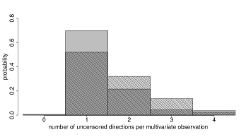
Figure 3. Average number of exactly observed coordinates above threshold in each recorded multivariate excess in the real data set (hatched bars) and in a simulated data set (Gray bars).

In addition to data above threshold, the number of threshold-overlapping blocks (made of data which position with respect to the threshold is undetermined, see Section 3) is $\mathcal{I}^{\prime}=39$ in this simulated data set, with block sizes varying between $1$ and $39\,845$, and a total number of ‘undetermined’ days $n^{\prime}_{\mathbf{v}}=112\,676$. To fix ideas, the bi-variate projections onto the six pairs $(i<j)$ of a simulated data set are displayed in Figure 4.

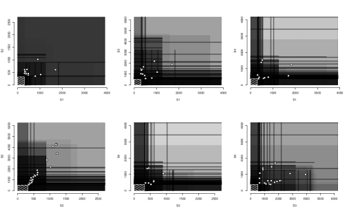
Figure 4. Bi-variate projection of the simulated data set after censoring. White points correspond to pairs for which both coordinates are observed. Superimposed Gray rectangles (resp. segments) represent pairs for which both coordinates (resp. one coordinate) are (is) censored. The white striped rectangle is the region below the multivariate threshold $\mathbf{v}$.

Let us turn to results obtained with this particular data set. A ‘flat’ prior was specified for the DM Poisson model parameters and MCMC proposals for the DM parameter were set in a similar way as in Sabourin and Naveau, (2014), which resulted in satisfactory convergence diagnostics after $10^{6}$ iterations, see Appendix D.6 for details. Figure 5 displays the posterior predictive for bi-variate marginalization’s of the angular density, obtained via equation (B.2), together with the true density and posterior credible sets around the estimates. The estimated density captures reasonably well the features of the true one and the posterior quantiles are rather concentrated around the true density. This is all the more satisfying that, at first view (Figure 4), the censored data used for inference seem to convey little information about the distribution of the angular components.

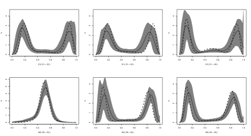
Figure 5. Bi-variate angular predictive densities (thick black line) with posterior credible sets (Gray regions) corresponding to the posterior $0.05-0.95$ quantiles, together with the true angular density (dashed line).

In risk analysis, especially in hydrology, return level plots (i.e. quantile plots) are used to summarize the marginal behavior of extremes. The return level $Q$ for a return period $T$ at location $j$, when marginal data are distributed according to $F_{j}^{\chi}$ and where there is no temporal dependence, is usually defined as the $1-1/T$-quantile of $F_{j}^{\chi}$. Figure 6 compares the return levels obtained both in the dependent and the independent models, together with the true return levels. The posterior estimates in the dependent model are very close to the truth, relatively to to the size of the credible intervals. In contrast, estimation in the independent model under-estimates the return levels, and the true curve lies outside the posterior quantiles at two locations out of four. This single example is however not enough to conclude that the dependence structure improves significantly marginal estimation. The absence of significant improvement (or deterioration) of marginal estimates is indeed one of the conclusions of the next subsection.

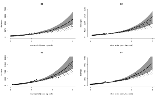
Figure 6. Return level plots: Quantile versus logarithm (base $10$) of the return period at the four locations. Grey points: empirical return level of observed threshold excesses (simulated data); Black line: true curves; Gray dashed line and shaded area: posterior mean and $0.05-0.95$-quantiles in the dependent model with Dirichlet mixture angular structure; Black dash-dotted line and area: idem in the independent model.

5.3. Simulation study with 50 data sets

The aim of this section is to verify that the posterior distribution of the DM Poisson model parameters is reasonably informative, even with censored data. The procedure described above is applied to generate independently 50 data sets.

Marginal predictive performance

The model’s ability to estimate of the probability of a marginal excess is first investigated. Large thresholds $(V_{1},\dotsc,V_{4})$ are specified so that their true marginal probability of exceedance is $P_{0}=1/(10*365)$, an approximate ten years return level. The quantities of interest are the posterior distributions of $\Delta_{j}(\theta)=\mathbb{P}_{\theta}(Y_{j}>V_{j})$, which we hope to be concentrated around $P_{0}$. Each posterior samples $(\theta_{\iota})_{\iota\in 1..N}$ issued by a MCMC algorithm is transformed into a series of exceedance probabilities, $(\delta_{j}(\theta_{\iota}))_{\iota\in 1..N}$ which empirical distribution $\hat{F}_{j}=\frac{1}{N}\sum_{\iota=1}^{N}\mathds{1}_{\delta_{j}(\theta_{\iota})}(\,\cdot\,)$ approximates the posterior distribution of $\Delta_{j}$. The performance of the posterior may then be investigated in terms of posterior quadratic loss,

$$\text{QL}(\hat{F}_{j}) =\big{(}\mathbb{E}_{\hat{F}_{j}}(\Delta_{j})-P_{0}\big{)}^{2}+\mathbb{V}\mathrm{ar}_{\hat{F}_{j}}(\Delta_{j})\,.$$

This loss corresponds to the the predictive model choice criterion (PMCC) (Laud and Ibrahim,, 1995). In the framework of scoring rules (Gneiting and Raftery,, 2007) the PMCC is not a ‘proper score’ in general, but it is so when the true probability distribution of the quantity of interest $\Delta_{j}$ is a Dirac mass, which is the case here (Dirac mass at $P_{0}$).

After $1.10^{6}$ MCMC iterations, at least one chain (out of six chains run in parallel for each simulated data set) passed the Heidelberger and Welch’s stationarity tests (Heidelberger and Welch,, 1983) at level $10^{-4}$, for each data set. Table 1 gathers, for the margins $j\in\{1,\dotsc,4\}$, the mean and standard deviation of the QL scores, normalized by the (squared) true probability $P_{0}^{2}$ for readability,

$$\overline{\text{QL}}_{j} =\frac{\text{QL}(\hat{F}_{j})}{P_{0}^{2}}\,.$$

$\overline{\text{QL}}_{j}$	1	2	3	4
mean	0.55	0.17	0.22	0.32
standard error	0.64	0.14	0.18	0.30
first quartile	0.14	0.08	0.08	0.10
third quartile	0.77	0.20	0.32	0.45

Table 1. Normalized scores $\overline{\text{QL}}_{j}$ for the marginal probability of an excess: mean and standard deviation, first and third quartiles over the $50$ data sets. Column $j$ corresponds to an excess at location $j$ ($1\leq j\leq 4$).

Although the variability of the scores (standard deviations) is relatively high, normalized third quartile less than one indicate that the posterior distribution concentrates in regions where the probability of a marginal excess is of the same order of magnitude as the true probability.

In order to verify that introducing a rather complex dependence structure model does not deteriorate the marginal estimates, the same quadratic loss score is computed with samples issued from the independent model. In view of Figure 7, displaying box-plots of the scores computed in both models (dependent versus independent), there is no significant difference between the two models in terms of marginal estimation.

Figure 7. Normalized QR scores in the dependent Dirichlet-Poisson model versus the independent model, at the four different locations, for 50 simulated datasets

Estimation of the angular measure

To assess the performance of the DM Poisson model in terms of estimation of the dependence structure of extremes, a similar scoring procedure as above is followed, with quantities of interest $\Delta_{j}$ defined as the probability of a joint excess of the $V_{i}$’s, given a marginal excess of $V_{j}$,

$$\tilde{\Delta}_{j}=\mathbb{P}(Y_{1}\geq V_{1},\dotsc Y_{4}\geq V_{4}\;|Y_{j}\geq V_{j})\,.$$

These quantities do not have an explicit expression in the DM model, but are easily approached by standard Monte-Carlo sampling. Lacking a reference model in this context (the independent one is obviously unable to predict these quantities), only the scores in the dependent model are available. Table 2 summarizes the results in terms of normalized scores

$$\tilde{\text{QL}}_{j}=\frac{\text{QL}(\tilde{\Delta}_{j})}{P_{j}^{2}}\,,$$

where $P_{j}$ is the true conditional probability of a joint excess.

$\tilde{\text{QL}}_{j}$	1	2	3	4
mean	0.06	0.18	0.25	0.05
standard error	0.05	0.11	0.13	0.05
first quartile	0.02	0.11	0.17	0.01
third quartile	0.10	0.23	0.33	0.06

Table 2. Normalized QL scores $\tilde{\text{QL}}_{j}$ for conditional probabilities of a joint excess: mean, standard deviation, first and third quartiles over the 50 simulated datasets. Column $j$ corresponds to conditioning upon an excess at location $j$.

A comforting fact is that the dependence structure seems to be even better estimated than the marginal distributions of extremes, in view of Tables 1 and 2.

5.4. Real data

Analyzing the hydrological data set presented in the introduction requires an additional declustering step: a multivariate run-declustering scheme was implemented. A cluster starts when one component exeeds the threshold. It and ends when, during $\tau$ consecutive days, all components are below there respective threshold, or (when censoring is present) with undertermined position, so that the observer can not ascertain that an excess occurred. The lag parameter $\tau=3$ was set by considering stability regions of the estimates, and additional physical characteristics of the hydrological catchment, see Sabourin and Renard, (2014) for details. After-wise the model is fitted to the extracted four-variate cluster maxima. Again, $6$ parallel MCMC’s of length $10^{6}$ are run, with satisfactory convergence diagnostic after a $2\,10^{5}$ burn-in period. The posterior mean estimates of marginal parameters are close to the maximum likelihood estimates mentioned in subsection 5.1. Figure 8 displays bi-variate versions of the four-variate posterior predictive angular measure, together with point-wise $90\%$ posterior credibility sets.

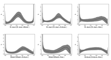
Figure 8. Bi-variate angular measure for the hydrological data set: posterior predictive density (black line) and posterior $0.05$ and $0.95$ quantiles.

The inferred dependence structure is rather complex, which fosters the use of such a flexible semi-parametric model. The posterior credible bounds of the angular density are relatively narrow around the posterior predictive in the central regions of the simplex (which is the segment $[0,1]$ for bi-variate data) and indicate that asymptotic dependence is present. On the other hand, high levels (even unboundedness) of the predictive density near certain edges indicates a ‘weakly asymptotically dependent regime’, for the considered pair, i.e.  a regime where one component may be large while the other one is not. Possibly, some ‘true’ asymptotic angular mass is concentrated on these edges, which translates in the Dirichlet mixture model (which only allows mass on the topological interior of the simplex) into high densities near the edges. The observed widening of posterior credible regions near the edges where the density is unbounded is not surprising : an unbounded density corresponds to Dirichlet parameters with components $\nu\mu_{i}<1$, for which a small variation of the parameter value induces a large variation of the density near the edges.

6. Conclusion

In this work, a flexible semi-parametric Bayesian inferential scheme is implemented to estimate the joint distribution of excesses above multivariate high thresholds, when the data are censored. A simulation example is designed on the same pattern as a real case borrowed from hydrology. Although the tuning of the MCMC algorithm requires some care, taking into account all kinds of observations for various censoring bounds allows to obtain satisfactory estimates, despite the loss of information relative to the angular structure induced by the censoring process. In particular, accurate enough estimations of quantities of interest such as marginal or conditional probabilities of an excess of a large threshold can be obtained.
The main methodological novelty consists in taking advantage of the conditioning and marginalizing properties of the Dirichlet distributions, in order to simulate augmentation data which ‘replace’ the missing ones. Also, exponential terms in the likelihood with no explicit expressions are handled by sampling well chosen functionals of augmentation Poisson processes. This new inferential framework opens the road to statistical analysis of the extremes of data sets that would otherwise have been deemed unworkable.

Appendix A Poisson likelihood of uncensored data

Consider a Dirichlet mixture density $h=h_{\psi}$ as in (2.3). The density of the exponent measure in Cartesian coordinates is, using (2.7) and the expression of the Dirichlet density (2.2),

$$\frac{\,\textup{d}\lambda_{\psi}}{\,\textup{d}\mathbf{x}}(\mathbf{x})=d\sum_{m=1}^{k}\left\{\frac{\mathit{p}_{m}\Gamma(\nu_{m})}{\prod_{j=1}^{d}\Gamma(\nu_{m}\,\mu_{j,m})}\prod_{j=1}^{d}x_{j}^{\nu_{m}\mu_{j,m}-1}\left(\sum_{j=1}^{d}x_{j}\right)^{-(\nu_{m}+1)}\right\}\,.$$ (A.1)

The likelihood expression (2.8) is simply that of a Poisson process on the region $[0,1]\times A_{\boldsymbol{u},n}$. Recall that, for a Poisson process with intensity $\mu$ on a region $A$, the likelihood of $n$ points $(Z_{1},\dotsc,Z_{n})$ observed in $A$ is proportional to $e^{-\mu(A)}\prod_{i=1}^{n}\frac{\,\textup{d}\mu}{\,\textup{d}z}(Z_{i})$.

The exponential term $e^{-n\,\lambda_{\psi}(A_{\boldsymbol{u}})}$ in (2.8) follows from the homogeneity property of $\lambda_{\psi}$,

$$e^{-\ell([0,1])\,.\,\lambda_{\psi}(A_{\boldsymbol{u},n})}=e^{-n\lambda_{\psi}(A_{\boldsymbol{u}})}\,.$$

The terms $J_{j}^{\chi}$ are the inverse Jacobians of the marginal transformations $T_{j}^{\chi}:Y_{j}\mapsto X_{j}$, i.e.

$$J_{j}^{\chi}(y_{j})=\sigma_{j}^{-1}(\zeta_{j})^{-\xi_{j}}x_{j}^{2}e^{\frac{1}{x_{j}}}\left[1-e^{\frac{-1}{x_{j}}}\right]^{1+\xi_{j}}\,,$$

where $x_{j}=\mathcal{T}_{j}^{\chi}(y_{j})$,

Appendix B Integration of the exponent measure along directions of missing components

The exact expression for the integral of the exponent measure’s density in (3.2) along the axes $[0,\infty]$ corresponding to missing coordinates is given below. Let $\mathscr{D}=\{j_{1},\dotsc,j_{r}\}$ be the non missing coordinates ($r<d$). Integrating $\frac{\,\textup{d}\lambda_{\psi}}{\,\textup{d}\mathbf{x}}$ over $(0,\infty)$ in the missing directions $\mathscr{D}_{0}=i_{1},\dotsc,i_{d-r}$ yields the marginal density of $\lambda$ with respect to the Lebesgue measure on the vector space spanned by $\mathscr{D}$, i.e. $\frac{\partial\lambda_{\psi}(\mathbf{x})}{\partial x_{j_{1}}\dotsb\,\partial x_{j_{r}}}$. With a DM angular measure, the integral has an analytic expression, which is, using (2.2) and (2.3),

$$\frac{\partial\lambda_{\psi}(\mathbf{x})}{\partial x_{j_{1}}\dotsb\partial x_{j_{r}}} =\int_{\{\mathbf{z}:z_{j}=x_{j}(j\in\mathscr{D}),z_{i}\in\mathbb{R}^{+}(i\in\mathscr{D}_{0})\}}\frac{\,\textup{d}\lambda_{\psi}}{\,\textup{d}\mathbf{x}}(\mathbf{z})\,\textup{d}z_{i_{1}},\dotsc,\,\textup{d}z_{i_{d-r}}$$ (B.1)

$$=r\sum_{m=1}^{k}\left(\frac{\mathit{p}_{m}^{0}\Gamma(\nu_{m}^{0})}{\prod_{j\in\mathscr{D}}\Gamma(\nu_{m}^{0}\mu_{j,m}^{0})}\prod_{j\in\mathscr{D}}x_{j}^{\nu_{m}^{0}\mu_{j,m}^{0}-1}\left(\sum_{j\in\mathscr{D}}x_{j}\right)^{-(\nu_{m}^{0}+1)}\right)\,,$$

with

$$\begin{gathered}\nu_{m}^{0}=\nu_{m}(1-\sum_{i\in\mathscr{D}_{0}}\mu_{i,m})\;,\quad\boldsymbol{\mu}_{m}^{0}=(1-\sum_{i\in\mathscr{D}_{0}}\mu_{i,m})^{-1}\boldsymbol{\mu}_{m}\;,\\ \mathit{p}_{m}^{0}=\frac{d}{r}(1-\sum_{i\in\mathscr{D}_{0}}\mu_{i,m})\mathit{p}_{m}\;.\end{gathered}$$ (B.2)

This is the spectral measure associated with another angular DM distribution on $\mathbf{S}_{r}$ with parameter $\psi^{0}=(\nu^{0}_{1:k},\boldsymbol{\mu}_{1:k}^{0},\mathit{p}_{1:k}^{0})$. The censored likelihood (3.2) can thus be re-written as

$$\mathcal{L}_{\mathbf{v}}(\mathbf{O},\theta) =\exp\Big{[}-n_{\text{det}}\,\lambda_{\psi}(A_{\boldsymbol{u}})-\sum_{i=1}^{\mathcal{I}^{\prime}}n^{\prime}_{i}\lambda_{\psi}(A^{\prime}_{i})\Big{]}\times\dotsb$$ (B.3)

$$\dotsb\,\prod_{i=1}^{n_{\mathbf{v}}}\Big{\{}\int_{\mathbf{[}\mathbf{\tilde{L}}_{t_{i}}^{0}\mathbf{,\tilde{R}}_{t_{i}}^{0}\mathbf{]}}\frac{\partial^{r(i)}\lambda_{\psi}}{\partial x_{j_{1}(t_{i})}\dotsb\partial x_{j_{r(i)}(t_{i})}}(\mathbf{x})\,\textup{d}\ell_{i}^{0}\prod_{j:Y_{j,t_{i}}>v_{j}}J_{j}^{\chi}(y_{j,t_{i}})\Big{\}}\,,$$

where integration is performed in the censored, non-missing directions, and where $\ell_{i}^{0}$ is the Lebesgue measure on the corresponding subspace of $\mathbb{R}^{d}$ and $\mathbf{[}\mathbf{\tilde{L}}_{t_{i}}^{0}\mathbf{,\tilde{R}}_{t_{i}}^{0}\mathbf{]}$ are the original bounds $\mathbf{[}\mathbf{\tilde{L}}_{t_{i}}\mathbf{,\tilde{R}}_{t_{i}}\mathbf{]}$, modulo the subspace of missing components.

Appendix C Data augmentation details

Here is detailed the construction of augmentation data $\mathbf{Z}=(\mathbf{Z}_{\text{above}},\mathbf{Z}^{\prime})$, first introduced in Section 4.2.

C.1. Definition of augmentation the variable $\mathbf{Z}_{\text{above}}=\{\mathbf{Z}_{t_{i}}\}_{i\leq n_{\mathbf{v}}}$

Consider a Fréchet-transformed, censored observation $\mathbf{C}_{t_{i}}^{\chi}=(C_{1}^{\chi},\dotsc,C_{d}^{\chi})$, with

$$C_{j}^{\chi}=(\tilde{\kappa}_{j,t_{i}},X_{j,t_{i}},\tilde{L}_{j,t_{i}},\tilde{R}_{j,t_{i}}),$$

as in Section 3.3. Let $\mathscr{D}_{c}(i)=(j^{\prime}_{1}(i),\dotsc,j^{\prime}_{c}(i))$ be the censored coordinates in observation $\mathbf{C}^{\chi}_{t_{i}}$. The latent variables $\mathbf{Z}_{t_{i}}=(Z_{j^{\prime}_{1},t_{i}},\dotsc,Z_{j^{\prime}_{c},t_{i}})$ are defined so as to ‘replace’ those coordinates: More formally, let

$$\mathbf{\bar{X}}_{t_{i}}\,|\,\psi\,\sim\frac{1}{\lambda_{\psi}(A_{\boldsymbol{u}})}\,\mathds{1}_{A_{\boldsymbol{u}}}(\,\cdot\,)\,\lambda_{\psi}(\,\cdot\,)\,,$$ (C.1)

be an uncensored $d$-dimensional variable with Fréchet margins and dependence structure given by $\lambda_{\psi}$ on $A_{\boldsymbol{u}}$. Then, $\mathbf{Z}_{t_{i}}$ is defined through its joint distribution with the $\{X_{j,t_{i}}\;:\;j\notin\mathscr{D}_{c}(i)\}$, conditionally on $\theta$,

$$\Big{(}\mathbf{Z}_{t_{i}},\{X_{j,t_{i}}\;:\;j\notin\mathscr{D}_{c}(i)\}\Big{)}\,\big{|}\,\theta\,\quad\overset{\text{distribution}}{=}\quad\mathbf{\bar{X}}_{t_{i}}\,|\psi.$$

Then, conditionally on the observation $\mathbf{O}_{t_{i}}$,

$$\big{[}\mathbf{Z}_{t_{i}}\,|\,\mathbf{O}_{t_{i}},\theta\,\big{]} =[(\bar{X}_{j^{\prime}_{1},t_{i}},\dotsc,\bar{X}_{j^{\prime}_{c},t_{i}})\;|\;\mathbf{O}_{t_{i}},\theta]$$ (C.2)

$$=\Big{[}(\bar{X}_{j^{\prime}_{1},t_{i}},\dotsc,\bar{X}_{j^{\prime}_{c},t_{i}})\Big{|}\;\mathbf{\bar{X}}_{t_{i}}\in\mathbf{[\tilde{L}}_{t_{i}},\mathbf{\tilde{R}}_{t_{i}}\mathbf{]},\;\psi\;\Big{]}\,.$$

The contribution of the ‘augmented’ data point $(\mathbf{Z}_{t_{i}},\mathbf{O}_{t_{i}})$ to the augmented likelihood (4.4) is

$$[\mathbf{z}_{t_{i}},\mathbf{O}_{t_{i}}|\theta]=\frac{\,\textup{d}\lambda_{\psi}}{\,\textup{d}x}(\mathbf{\bar{x}}_{t_{i}})\prod_{j:\kappa_{j,t_{i}}=1}J_{j}^{\chi}(y_{j,t_{i}})\,,$$ (C.3)

where

$$\bar{x}_{j,t_{i}}=\begin{cases}\mathcal{T}_{j}^{\chi}(y_{j,t_{i}})&\text{if }\tilde{\kappa}_{j,t_{i}}=1\,,\\ z_{j,t_{i}}&\text{otherwise .}\end{cases}$$

Remark.

With missing components $\mathcal{D}_{0}(i)=\{j:\kappa_{j,t_{i}}=0\}\neq\emptyset$, integration in the direction $\mathcal{D}_{0}(i)$ can be performed analytically (see Appendix B), which reduces the dimension of the augmented data. Indeed, in such a case, the corresponding $Z_{j,t_{i}}$’s need not be included in $\mathbf{Z}_{t_{i}}$, the uncensored variable $\mathbf{\bar{X}}_{t_{i}}$ is defined on the quotient spaces $\mathbf{E}/\mathcal{D}_{0}(i)$ and its distribution is proportional to the exponent measure $\lambda_{\psi^{0}}$ defined by equations (B.1) and (B.2), with density $\frac{\partial^{r(i)}\lambda_{\psi}}{\partial x_{j_{1}(t_{i})}\dotsb\,\partial x_{j_{r(i)}(t_{i})}}(\,\cdot\,)\,.$ as in equation (B.3), so that

$$[\mathbf{z}_{t_{i}},\mathbf{O}_{t_{i}}|\theta]=\frac{\partial^{r(i)}\lambda_{\psi}}{\partial x_{j_{1}(t_{i})}\dotsb\,\partial x_{j_{r(i)}(t_{i})}}(\mathbf{\bar{x}}_{t_{i}})\prod_{j:\kappa_{j,t_{i}}=1}J_{j}^{\chi}(y_{j,t_{i}})\,,$$ (C.4)

C.2. Full conditional distribution of augmented data $[\,\mathbf{Z}_{\text{above}}\,|\,\mathbf{O},\theta\,]$

The full conditionals $[Z_{j,t_{i}}|\{Z_{s,t_{i}}\}_{s\neq j},\mathbf{O}_{t_{i}},\theta]$ are functions of truncated Beta distributions that can easily be sampled in a Gibbs step of the algorithm, as shown below.

In the remaining of this subsection, we omit the temporal index $t_{i}$. If $\psi$ is a mixture of $k$ Dirichlet distributions, as in (2.3), then, for any bounded, continuous function $g$ defined on $[\tilde{L}_{j},\tilde{R}_{j}]$, the conditional expectation of $g(Z_{j})$ is, up to a multiplicative constant,

$$\mathbb{E}\left[g(Z_{j})\left|\mathbf{O},\{Z_{r}\}_{r\neq j},\theta\right.\right] =\mathbb{E}\left[g(\bar{X}_{j})\left|\bar{X}_{j}\in[\tilde{L}_{j},\tilde{R}_{j}],\bar{X}_{r}=x_{r}\,(r\neq j),\,\psi\right.\right]$$ (C.5)

$$=\int_{\tilde{L}_{j}}^{\tilde{R}_{j}}g(x_{j})h_{\psi}\Big{(}\frac{\mathbf{x}}{\sum_{r}x_{r}}\Big{)}\Big{(}\sum_{r}x_{r}\Big{)}^{-(d+1)}\,\textup{d}x_{j}$$

$$=\sum_{m=1}^{k}\mathit{p}_{m}\underbrace{\int_{\tilde{L}_{j}}^{\tilde{R}_{j}}g(x_{j})h_{\psi,m}\Big{(}\frac{\mathbf{x}}{\sum_{r}x_{r}}\Big{)}\Big{(}\sum_{r}x_{r}\Big{)}^{-(d+1)}\,\textup{d}x_{j}}_{I_{m}}\,,$$

(see equation (C.1) for the definition of $\bar{X}_{j}$).

Each term $I_{m}$ ($m\leq k$ for a mixture of $k$ components) is

$$I_{m} =\gamma_{m}\int_{\tilde{L}_{j}}^{\tilde{R}_{j}}g(x_{j})\prod_{r\leq d}x_{r}^{\nu_{m}\,\mu_{r,m}-1}\left(\sum_{r\leq d}x_{r}\right)^{-(d+1)-(\sum_{r\leq d}(\nu_{m}\,\mu_{r,m}-1))}\,\textup{d}x_{j}$$

$$=\gamma_{m}\int_{\tilde{L}_{j}}^{\tilde{R}_{j}}g(x_{j})\prod_{r\leq d}x_{r}^{\nu_{m}\,\mu_{r,m}-1}\left(\sum_{r\leq d}x_{r}\right)^{-(\nu_{m}+1)}\,\textup{d}x_{j}$$

$$=\gamma_{m}\,\rho_{j}\int_{\tilde{L}_{j}}^{\tilde{R}_{j}}g(x_{j})x_{j}^{\nu_{m}\mu_{j,m}-1}(s_{j}+x_{j})^{-\nu_{m}-1}\,\textup{d}x_{j}\,,$$

where $\gamma_{m}=\frac{\Gamma(\nu_{m})}{\prod_{r=1}^{d}\Gamma(\nu_{m}\mu_{r,m})}$, $s_{j}=\sum_{r\neq j}x_{r}$ and $\rho_{j}=\prod_{r\neq j}x_{r}^{\nu_{m}\mu_{r,m}-1}$. Changing variable with $u=x_{j}/(x_{j}+s_{j})$, the integration bounds are

$$R^{\prime}_{j}=\frac{\tilde{R}_{j}}{s_{j}+\tilde{R}_{j}}\,,\;L^{\prime}_{j}=\frac{\tilde{L}_{j}}{s_{j}+\tilde{L}_{j}},$$

and we have

$$I_{m} =\gamma_{m}\,\rho_{j}\,\int_{L^{\prime}_{j}}^{R^{\prime}_{j}}g\left(\frac{s_{j}u}{1-u}\right)\,\left(\frac{s_{j}u}{1-u}\right)^{\nu_{m}\mu_{j,m}-1}(s_{j}+\frac{s_{j}u}{1-u})^{-\nu_{m}-1}\frac{s_{j}}{(1-u)^{2}}\,\textup{d}u$$

$$=\gamma_{m}\,\rho_{j}\,s_{j}^{-\nu_{m}(1-\mu_{j,m})-1}\int_{L^{\prime}_{j}}^{R^{\prime}_{j}}g\left(\frac{s_{j}u}{1-u}\right)\,u^{\nu_{m}\mu_{j,m}-1}(1-u)^{\nu_{m}(1-\mu_{j,m})}\,\textup{d}u$$

One recognizes in the integrand the unnormalized density of a Beta random variable $U_{m}~{}\sim~{}\operatorname{beta}(a_{m},b_{m})$, with

$$a_{m}=\nu_{m}\mu_{j,m}\,,\quad b_{m}=\nu_{m}(1-\mu_{j,m})+1\,;$$

Let $\mathrm{IB}_{a,b}(x,y)$ denote the incomplete Beta function (i.e. the integral of the Beta density) between truncation bounds $x$ and $y$. The missing normalizing constant in the integrand is

$$D_{m} =\frac{\Gamma(a_{m}+b_{m})}{\Gamma(a_{m})\Gamma(b_{m})\mathrm{IB}_{a_{m},b_{m}}(L^{\prime}_{j},R^{\prime}_{j})}$$

$$=\frac{\Gamma(\nu_{m})}{\Gamma(\nu_{m}\mu_{j,m})\Gamma(\nu_{m}(1-\mu_{j,m}))}\frac{1}{\mathrm{IB}_{a_{m},b_{m}}(L^{\prime}_{j},R^{\prime}_{j})(1-\mu_{j,m})}$$

Finally, we have

$$I_{m}=C_{m}.D_{m}\int_{L^{\prime}_{j}}^{R^{\prime}_{j}}g(\frac{s_{j}u}{1-u})\,u^{\nu_{m}\mu_{j,m}-1}(1-u)^{\nu_{m}(1-\mu_{j,m})}\,\textup{d}u$$

with

$$C_{m}=(1-\mu_{j,m})\frac{\Gamma(\nu_{m}(1-\mu_{j,m}))}{\prod_{s\neq j}\Gamma(\nu_{m}\mu_{s,m})}\mathrm{IB}_{a_{m},b_{m}}(L^{\prime}_{j},R^{\prime}_{j})\,\rho_{j}\,s_{j}^{-\nu_{m}(1-\mu_{j,m})-1},$$ (C.6)

so that that the conditional expectation (C.5) is that of a mixture distribution,

$$\mathbb{E}\left[g(Z_{j})|\mathbf{O},\{Z_{r,r\neq j}\}\right]=\sum_{m=1}^{j}\,p^{\prime}_{m}\,\mathbb{E}\left[g(\frac{s_{j}U_{m}}{1-U_{m}})\right]$$

with weights $(p^{\prime}_{m})_{m\leq k}$,

$$p^{\prime}_{m}=\mathit{p}_{m}\,C_{m}\,,$$ (C.7)

where $C_{m}$ is given by equation (C.6).

As a conclusion, the conditional variable $[Z_{j}|\mathbf{O},Z_{s\neq j},\theta]$ is a mixture distribution of $k$ components

$$\left(p^{\prime}_{m},V_{j,m}=\frac{s_{j}U_{m}}{1-U_{m}}\right)_{1\leq m\leq k}\,.$$ (C.8)

In presence of missing coordinates, (C.8) still holds, up to replacing the mixture parameters $(\mathbf{p},\boldsymbol{\mu},\boldsymbol{\nu})$ with $(\mathbf{p}^{0},\boldsymbol{\mu}^{0},\boldsymbol{\nu}^{0})$ as in equation (B.2).

C.3. Augmentation Poisson process $\mathbf{Z}^{\prime}=\{\{\mathbf{Z}^{\prime}_{i}\}_{i\leq\mathcal{I}^{\prime}},\mathbf{Z}^{\prime}_{\boldsymbol{u}}\}$ and weight function $\varphi$

Let us define a region $E_{\boldsymbol{u},n_{\text{det}}}=\{\mathbf{x}\in(\mathbb{R}^{+})^{d}:\|\mathbf{x}\|_{1}>\min_{j}(\frac{u_{j}}{n_{\text{det}}})\}$, so that $A_{\boldsymbol{u},n_{\text{det}}}\subset E_{\boldsymbol{u},n_{\text{det}}}$. Choose a multiplicative constant $\tau>0$ and define a Poisson intensity measure $\lambda^{\prime}(\,\cdot\,)=\tau\,\lambda_{\psi}(\,\cdot\,)$. The augmentation process $\mathbf{Z}^{\prime}_{\boldsymbol{u}}$ is a Poisson processes which is defined together with $\varphi_{\boldsymbol{u}}$ by

$$\begin{cases}\mathbf{Z}^{\prime}_{\boldsymbol{u}}\sim\operatorname{PP}(\lambda^{\prime})\text{ on }E_{\boldsymbol{u},n_{\text{det}}}\,,\\ \varphi_{\boldsymbol{u}}(\mathbf{Z}^{\prime}_{\boldsymbol{u}})=(1-1/\tau)^{\mathbf{Z}^{\prime}_{\boldsymbol{u}}(A_{\boldsymbol{u},n_{\text{det}}})}\,,\end{cases}$$ (C.9)

where $\mathbf{Z}^{\prime}_{\boldsymbol{u}}(A_{\boldsymbol{u},n_{\text{det}}})$ is the number of points forming $\mathbf{Z}^{\prime}_{\boldsymbol{u}}$ which hit $A_{\boldsymbol{u},n_{\text{det}}}$. Full justification and simulation details are given in the next subsection (Appendix C.4).

Let $\{\mathbf{x}^{\prime}_{\boldsymbol{u},s}=(r^{\prime}_{\boldsymbol{u},s},\mathbf{w}^{\prime}_{\boldsymbol{u},s})\}_{s\leq N^{\prime}_{\boldsymbol{u}}}$ be the points of $\mathbf{Z}^{\prime}_{\boldsymbol{u}}$ in $E_{\boldsymbol{u},n_{\text{det}}}$, the density of $\mathbf{Z}^{\prime}_{\boldsymbol{u}}$ over $E_{\boldsymbol{u},n_{\text{det}}}$, which contributes to the augmented likelihood (4.4), is

$$[\mathbf{z}^{\prime}_{\boldsymbol{u}}\mid\psi]=\frac{1}{N^{\prime}_{\boldsymbol{u}}!}\;e^{\frac{-n_{\text{det}}\,\tau\,d}{\min_{j\leq d}\boldsymbol{u}_{j}}}\prod_{s=1}^{N^{\prime}_{\boldsymbol{u}}}\frac{\tau\,d}{(r^{\prime}_{\boldsymbol{u},s})^{2}}h_{\psi}(\mathbf{w}^{\prime}_{\boldsymbol{u},s})\,.$$ (C.10)

The processes $\mathbf{Z}^{\prime}_{i}$’s and the weights $\varphi^{\prime}_{i}$’s are defined similarly, replacing $n_{\text{det}}$ with $n^{\prime}_{i}$ and $u_{j}$ with $\tilde{R}_{j,t^{\prime}_{i}}$ ($1\leq i\leq\mathcal{I}^{\prime}$).

C.4. Consistency of the augmentation model .

The augmentation process $\mathbf{Z}^{\prime}$ and the weight function $\varphi$ have been constructed with a hint towards using the general expression of the Laplace transform of a Poisson process to prove consistency of the augmented posterior.

Proposition 1.

Define the factors

$$[\,\mathbf{z}_{t_{i}},\mathbf{O}_{t_{i}}\,|\,\theta\,]\,(i\leq n_{\mathbf{v}})\quad\text{and}\quad[\,\mathbf{z}^{\prime}_{\boldsymbol{u}}\;|\;\psi],[\mathbf{z}^{\prime}_{i}\,|\,\psi]\;\;(1\leq i\leq\mathcal{I}^{\prime})$$

composing the augmented likelihood (4.4), according to equations (C.3) and (C.10), and let the factors $\varphi_{\boldsymbol{u}},\;\varphi_{i},\;i\leq\mathcal{I}^{\prime}$ of the weight function $\varphi$ in (4.2) be defined by equation (C.9).

Then, the augmented posterior $[\,\mathbf{z},\theta\,|\,\mathbf{O}\,]_{+}\propto[\,\theta\,][\mathbf{z},\mathbf{O}\,|\,\theta\,]\,\varphi(\mathbf{z})\$ is consistent, in the sense that condition (4.3), whence (4.1), is satisfied.

Proof

It is enough to show that, on the one hand,

$$\int[\mathbf{z}_{\text{above}},\mathbf{O}\;|\;\theta\,]\,\textup{d}\mathbf{z}_{\text{above}}=\prod_{i=1}^{n_{\mathbf{v}}}\Bigg{\{}\int_{\mathbf{[\tilde{L}}_{t_{i}},\mathbf{\tilde{R}}_{t_{i}}\mathbf{]}}\frac{\,\textup{d}\lambda_{\psi}}{\,\textup{d}\mathbf{x}}\,\textup{d}\ell_{i}(\mathbf{x})\prod_{j:y_{j,t_{i}}>v_{j}}J_{j}^{\chi}(y_{j,t_{i}})\,,\Bigg{\}}$$ (C.11)

and, on the other hand,

$$\begin{cases}\mathbb{E}\left[\varphi_{{\boldsymbol{u}}}(\mathbf{Z}^{\prime}_{\boldsymbol{u}})\right]=\exp\left(-n_{\text{det}}\,\lambda_{\psi}\left(A_{\boldsymbol{u}}\right)\right)\,,\\ \mathbb{E}\left[\varphi_{{i}}(\mathbf{Z}^{\prime}_{i})\right]=\exp\left(-n^{\prime}_{i}\,\lambda_{\psi}(A^{\prime}_{i})\right)&(i\leq\mathcal{I}^{\prime})\,.\end{cases}$$ (C.12)

where the above expectations are taken with respect to $[\mathbf{Z}^{\prime}_{\boldsymbol{u}}\,|\,\psi\,]$ and $[\mathbf{Z}^{\prime}_{i}\,|\,\psi\,]$.

Establishing (C.11) is immediate: from definition (C.3) of the $[\mathbf{z}_{t_{i}},\mathbf{O}|\theta]$’s composing $[\mathbf{z}_{\text{above}},\mathbf{O}|\theta]$,

$$\int_{\mathbf{[\tilde{L}}_{t_{i}},\mathbf{\tilde{R}}_{t_{i}}\mathbf{]}}[\mathbf{z}_{t_{i}},\mathbf{O}_{t_{i}}|\theta]\,\textup{d}\mathbf{z}_{t_{i}}=\int_{\mathbf{[\tilde{L}}_{t_{i}},\mathbf{\tilde{R}}_{t_{i}}\mathbf{]}}\frac{\,\textup{d}\lambda_{\psi}}{\,\textup{d}\mathbf{x}}\,\textup{d}\ell_{i}(\mathbf{x})\prod_{j:y_{j,t_{i}}>v_{j}}J_{j}^{\chi}(y_{j,t_{i}})\,,$$

which yields (C.11) by taking the product over indices $1\leq i\leq n_{\mathbf{v}}$.

It remains to show (C.12). To wit, $\varphi_{\boldsymbol{u}}$ is a smoothed version of the indicator function $\mathds{1}_{\{\mathbf{N}^{\prime}_{\boldsymbol{u}}(A_{\boldsymbol{u},n_{\text{det}}})=0\}}$, which expectancy is $\mathbb{P}(\mathbf{N}^{\prime}_{\boldsymbol{u}}(A_{\boldsymbol{u},n_{\text{det}}})=0)=e^{-n_{\text{det}}\lambda_{\psi}(A_{\boldsymbol{u}})}$, as soon as $\mathbf{N}^{\prime}_{\boldsymbol{u}}$ is a Poisson process with intensity measure $\lambda_{\psi}$. For $f$ a bounded, continuous function defined on a nice space $E$ and $N$ a point process on $E$, denote

$$N(f)=\int_{E}f\,\textup{d}N=\sum_{i=1}^{N(E)}f(s_{i}).$$

Then, if $N$ is a Poisson process $\operatorname{PP}(\lambda)$ on $E$, the Laplace transform $\mathit{Lap}_{N}(f)\hat{=}\mathbb{E}(e^{-N(f)})$ is (Resnick,, 1987, Chap. 3)

$$\mathit{Lap}_{N}(f)=\exp\left(-\int_{E}(1-e^{-f(s)})\,\textup{d}\lambda(s)\right)\,.$$

Consider the region $E=E_{\boldsymbol{u},n_{\text{det}}}$ as in (C.9) and take

$$f_{\boldsymbol{u}}(\mathbf{x})=-\log(1-1/\tau)\mathbf{1}_{A_{\boldsymbol{u},n_{\text{det}}}}(\mathbf{x})\,,\quad\text{ so that }\quad 1-e^{-f_{\boldsymbol{u}}}=\frac{1}{\tau}\mathds{1}_{A_{\boldsymbol{u},n_{\text{det}}}}\,.$$

With these notations,

$$\varphi_{\boldsymbol{u}}(\mathbf{Z}^{\prime}_{\boldsymbol{u}})\;\hat{=}\;\left(1-\frac{1}{\tau}\right)^{\mathbf{Z}^{\prime}_{\boldsymbol{u}}(A_{\boldsymbol{u},n_{\text{det}}})}\;=\;\exp\left(-\mathbf{Z}^{\prime}_{\boldsymbol{u}}(f_{\boldsymbol{u}})\right),$$

whence

$$\mathbb{E}\left(\varphi_{\boldsymbol{u}}(\mathbf{Z}^{\prime}_{\boldsymbol{u}})\right) =\mathit{Lap}_{\mathbf{Z}^{\prime}_{\boldsymbol{u}}}(f_{\boldsymbol{u}})$$

$$=\exp\left(-\int_{E_{\boldsymbol{u},n_{\text{det}}}}(1-e^{-f_{\boldsymbol{u}}})\,\textup{d}\lambda^{\prime}\right)$$

$$=\exp\left(-\int_{E_{\boldsymbol{u},n_{\text{det}}}}\frac{1}{\tau}\mathds{1}_{A_{\boldsymbol{u},n_{\text{det}}}}\,\textup{d}(\tau\lambda_{\psi})\right)$$

$$=\exp\left(-\lambda_{\psi}(A_{\boldsymbol{u},n_{\text{det}}})\right)\,.$$

This shows the first equality in (C.12). The second one is derived with a similar argument.

$\square$

The points of $\mathbf{Z}^{\prime}_{\boldsymbol{u}}$ can easily be simulated (see Resnick,, 1987, Chap.3): the number of points $N^{\prime}_{\boldsymbol{u}}$ in $E_{\boldsymbol{u},n_{\text{det}}}$ is a Poisson random variable with mean equal to

$$\lambda^{\prime}(E_{\boldsymbol{u},n_{\text{det}}})~{}=~{}\frac{\tau~{}d~{}}{\min_{j}(u_{j}~{}/n_{\text{det}})}\,,$$

and each point has density in polar coordinates equal to $\frac{1}{\lambda^{\prime}(E_{\boldsymbol{u},n_{\text{det}}})}\frac{\tau d}{r^{2}}h_{\psi}(\mathbf{w})$.

Remark.

One may be tempted to define $\mathbf{Z}^{\prime}_{\boldsymbol{u}}$ as a Poisson process with intensity $\lambda_{\psi}$ on some $E\supset A_{\boldsymbol{u},n_{\text{det}}}$, and $\varphi(\mathbf{Z}_{\boldsymbol{u}})$ as the indicator $\mathds{1}_{\mathbf{z}^{\prime}_{\boldsymbol{u}}(A_{\boldsymbol{u},n_{\text{det}}})=0}$, with a similar definition for the $\varphi_{i}^{\prime}$’s and the $\mathbf{Z}^{\prime}_{i}$’s. As pointed out in the proof of Proposition 1, one would have $\mathbb{E}\left[\mathbf{1}_{\mathbf{Z}^{\prime}_{u}(A_{\boldsymbol{u},n_{\text{det}}})=0}\right]=\exp\left(-n_{\text{det}}\,\lambda_{\psi}\left(A_{\boldsymbol{u}}\right)\right)$, as required. However, even if this construction is valid in theory, it leads to a very large rate of rejection in the Metropolis algorithm: $\varphi(\mathbf{Z}^{\prime}_{\boldsymbol{u}})$ has too much variability around its mean value and the proposal is systematically rejected each time a point in the augmentation process hits the failure region.

C.5. Expression of the augmented posterior

Recall from Section 4.2, equation (4.2), that the augmented posterior density to be sampled by the MCMC algorithm is

$$[\,\mathbf{z},\theta\,|\,\mathbf{O}\,]_{+}\propto[\,\theta\,][\,\mathbf{z},\mathbf{O}\,|\,\theta\,]\varphi(\mathbf{z})\,.$$

Combining equations (C.3) and (C.9), and integrating out missing components as in Appendix B, the developed expression is

$$[\,\mathbf{z},\,\theta\,|\,\mathbf{O}\,]_{+}\;\propto\;[\,\theta\,]\;\left([\mathbf{z}^{\prime}_{\boldsymbol{u}}|\psi]\prod_{i=1}^{\mathcal{I}^{\prime}}[\mathbf{z}^{\prime}_{i}|\psi]\right)\,\cdot\,(1-1/\tau)^{\mathbf{z}^{\prime}_{\boldsymbol{u}}(A_{\boldsymbol{u},n_{\text{det}}})+\sum_{i=1}^{\mathcal{I}^{\prime}}\mathbf{z}^{\prime}_{i}(A^{\prime}_{i,n^{\prime}_{i}})}\,\dotsb\\ \dotsb\prod_{i=1}^{n_{\mathbf{v}}}\Big{\{}\frac{\partial^{r(i)}\lambda_{\psi}}{\partial x_{j_{1}(i)}\dotsb x_{j_{r(i)}(i)}}(\mathbf{\bar{x}}_{t_{i}})\prod_{j:Y_{j,t}>v_{j}}J_{j}^{\chi}(y_{j,t})\Big{\}}\,,$$ (C.13)

where $[\mathbf{z}^{\prime}_{\boldsymbol{u}}|\psi]$ and the $[\mathbf{z}^{\prime}_{i}|\psi]$’s are given by equation (C.10).

Appendix D MCMC algorithm

The MCMC algorithm generates a sample $(\theta_{\iota},\mathbf{Z}_{\iota})_{\iota=1,\dotsc,N}$ which distribution converges to the invariant distribution of the chain, which is the augmented posterior distribution $[\mathbf{Z},\theta|\mathbf{O}]_{+}$, as defined in Section 4 and Appendix C.5. The quantity of interest here is the joint parameter $\theta$, which is the concatenation of the marginal parameters and the dependence parameter: $\theta=(\chi,\psi)$. We recall that MCMC algorithms aiming at sampling a quantity $\Delta\in E$ according to a density $\pi(\,\cdot\,)$ proceed typically as follows

• Start with any value $\delta(0)\in E$

• for $\iota\in\{1,\dotsc,N\}$

  1. Generate $\delta^{*}$ according to a proposal distribution with density $q(\delta(\iota),\,\cdot\,)$

  2. Compute the acceptance ratio

     $$\alpha=\frac{\pi(\delta^{*})\;q(\delta^{*},\delta(\iota))}{\pi(\delta(\iota))\;q(\delta(\iota),\delta^{*})}\;,$$

     and generate $U$, a uniform random variable on $[0,1]$.

  3. If $U>\alpha$, ‘reject’ the proposal and set

     $$\delta(\iota+1)=\delta(\iota)\,.$$

     Otherwise (i.e. with probability $\alpha$), set

     $$\delta(\iota+1)=\delta^{*}$$

  4. Set $\iota=\iota+1$, go to (1).

• Return $\Big{(}\delta(\iota_{\min}),\dotsc,\delta(N)\Big{)}$,

where $\iota_{\min}$ is the length of the burn-in period, after which the chain is deemed to have reached a stationary behavior. In our case, the unnormalized posterior measure $[\mathbf{Z},\theta|\mathbf{O}]_{+}$ (see equation (C.13)) on the augmented parameter space plays the role of the objective density $\pi$ above.

In a Metropolis-within-Gibbs MCMC, several proposal kernels $q_{1},\dotsc,q_{T}$ are defined, each of them corresponding to a type of move, which is randomly chosen among $\{1,\dotsc,T\}$ at each iteration $\iota$ and allows to modify some subset of components in $\delta$ alone. The algorithm developed in this paper builds on the MCMC algorithm proposed by Sabourin and Naveau, (2014), in which several types of move modifying the dependence structure (Dirichlet mixture parameter $\psi$) have been defined. Those are kept as they are in the present work, the novel part of which concerns the definition of marginal moves (modifying the marginal parameter $\chi$) and augmentation moves (modifying the augmentation data $\mathbf{Z}$). Additional notations distinguishing between the quantities appearing in the general MCMC algorithm above, according to the type of move, are omitted in the remainder of this section.

D.1. Starting values

In a preliminary step, likelihood optimization is performed in the independent model (the likelihood for one multivariate observation is the product of $d$ Pareto densities). This provides starting values for the marginal parameters as well as a Hessian matrix $\mathcal{H}$, that may be used as the inverse of a reference covariance matrix when updating the marginal parameters.

D.2. Marginal moves

The marginal parameter $\chi$ is updated as a block: The proposal is normal, with mean at $\chi(\iota)$ and co-variance matrix $\Sigma=\delta\,\mathcal{H}^{-1}$, where $\delta$ is a scaling factor fixed by the user, that may typically be set around $0.5$ and $\mathcal{H}$ is the Hessian matrix computed in the preliminary step. Since the proposal density is symmetric, and since this move does not modify the dependence structure, neither the terms involving the proposal density, nor the point processes $\mathbf{Z}^{\prime}$, appear in acceptance ratio. The augmented variables $\mathbf{Z}_{\text{above}}$ are left unchanged. If any augmented component $\mathbf{Z}_{j,t_{i}}$ is outside of the candidate censoring interval $\mathbf{[}\mathbf{\tilde{L}}_{t_{i}}^{*}\mathbf{,\tilde{R}}_{t_{i}}^{*}\mathbf{]}$ (on the new Fréchet scale) resulting from the modification of the marginal parameters, the move is rejected, since in such a case, the candidate has augmented likelihood $[\mathbf{z},\mathbf{O}\,|\,\theta^{*}\,]=0$, i.e. $\alpha=0$.

Otherwise, the uncensored Fréchet-transformed variables (such that $\tilde{\kappa}_{j,t_{i}}=1$) are updated to $\mathbf{{X}}_{t_{i}}^{*}=\mathcal{T}_{j,t_{i}}^{\chi^{*}}(Y_{j,t_{i}})$. The acceptance ratio is

$$\alpha=\frac{[\chi^{*}]}{[\chi(\iota)]}\prod_{i=1}^{n_{\mathbf{v}}}\Bigg{\{}\frac{\partial^{r(i)}\lambda_{\psi}}{\partial x_{j_{1}(i)}\dotsb\partial x_{j_{r(i)}(i)}}(\mathbf{\bar{X}}^{*}_{t_{i}})\left[\frac{\partial^{r(i)}\lambda_{\psi}}{\partial x_{j_{1}(i)}\dotsb\partial x_{j_{r(i)}(i)}}(\mathbf{\bar{X}}_{t_{i}}(\iota))\right]^{-1}\\ \prod_{j:Y_{j,t_{i}}>v_{j}}\frac{J_{j}^{\chi^{*}}(Y_{j,t_{i}})}{J_{j}^{\chi(\iota)}(Y_{j,t_{i}})}\Bigg{\}},$$

where $j_{1},\dotsc,j_{r(i)}$ are the non-missing components in the censored observation $\mathbf{C}_{t_{i}}^{\chi}$ and $\bar{X}_{j}=X_{j}$ for uncensored components, $\bar{X}_{j,t_{i}}=Z_{j,t_{i}}$ otherwise (see Appendix B).

D.3. Augmentation moves for $\mathbf{Z}_{\text{above}}$

The augmented components $\{Z_{j,t_{i}}\}=\{\bar{\mathbf{X}}_{j,t_{i}}:\tilde{\kappa}_{j}\in\{2,3\}\}$ (c.f. Section 4.2) are re-sampled, one coordinate at a time, from their exact conditional distribution given the other coordinates, as derived in Appendix  C.1. Since no other component of $(\mathbf{Z},\theta)$ is modified, the proposal density equals the objective density, and the acceptance ratio is thus set to $\alpha=1$.

D.4. Augmentation moves for $\mathbf{Z}^{\prime}$

During this move, proposals

$$\mathbf{Z}^{\prime*}=\left\{\mathbf{Z}^{\prime*}_{\boldsymbol{u}},\mathbf{Z}^{\prime*}_{i},\;i\leq\mathcal{I}^{\prime}\right\}\,,$$

for the augmentation Poisson processes introduced in the end of Section 3.4, are sampled under their exact distribution,

$$q\Big{(}\mathbf{Z}^{\prime}(\iota),\mathbf{Z}^{\prime*}\Big{)}=[\mathbf{Z}^{\prime*}|\psi(\iota)]\,.$$

The latter is determined by their intensity measure $\lambda^{\prime}=\tau\lambda_{\psi}$: the multiplicative constant $\tau$ and the sampling procedure have been described in Appendix C.3. The acceptance ratio is thus

$$\alpha=\frac{[\,\mathbf{Z}^{\prime*},\theta(\iota)\,|\,\mathbf{O}\,]_{+}\;\;[\,\mathbf{Z}^{\prime}(\iota)\,|\,\psi(\iota)\,]}{[\,\mathbf{Z}^{\prime*},\theta(\iota)\,|\,\mathbf{O}\,]_{+}\;\;[\,\mathbf{Z}^{\prime*}\,|\,\psi(\iota)\,]}$$

all the terms cancel out except the ratio $\varphi(\mathbf{Z}^{\prime*})/\varphi(\mathbf{Z}^{\prime}(\iota))$, so that

$$\alpha=(1-1/\tau)^{\left[(\mathbf{Z}^{\prime}_{\boldsymbol{u}})^{*}(A_{\boldsymbol{u},n_{\text{det}}})-\mathbf{Z}^{\prime}_{\boldsymbol{u}}(\iota)(A_{\boldsymbol{u},n_{\text{det}}})\right]+\sum_{i\leq\mathcal{I}^{\prime}}\left[(\mathbf{Z}^{\prime}_{i})^{*}(A^{\prime}_{i,n^{\prime}_{i}})-\mathbf{Z}^{\prime}_{i}(\iota)(A^{\prime}_{i,n^{\prime}_{i}})\right]}\,.$$

D.5. Dependence moves

These types of moves allow to update $\psi(\iota)$.The only difference between the present algorithm and what is described is Sabourin and Naveau, (2014) is that not enough exact angular data are available to construct proposals for moving or splitting a Dirichlet mixture components $\boldsymbol{\mu}_{m}$ . Indeed, most of the observations have at least one coordinate missing or censored, so that no ‘angle’ is available. Consequently, the latter proposal is a simple Dirichlet distribution with mode at $\boldsymbol{\mu}_{m}(\iota)$, with re-centering parameter $0<\epsilon<0.5$,

$$q(\boldsymbol{\mu}_{m}(\iota),\,\cdot\,)=\operatorname{diri}_{\frac{d}{\epsilon},\gamma^{*}}(\,\cdot\,)\,,$$

with $\gamma^{*}=(1-\epsilon)\,\boldsymbol{\mu}_{m}+\epsilon\,(\frac{1}{d},\dotsc,\frac{1}{d})$.

Each dependence move (except for a shuffling move which only affects the representation of the angular distribution, see Sabourin and Naveau, (2014)) is systematically followed by an augmentation move updating the Poisson processes $\mathbf{Z}^{\prime}$, which improves the chain’s mixing properties. This also avoids the computation of the ‘costly’ term involving the density $[\mathbf{z}^{\prime}|\psi]$ (see equation (C.10)). Indeed, the acceptance ratio for the two consecutive moves (dependence move followed by a augmentation move) is

$$\alpha=\frac{[\psi^{*}]}{[\psi(\iota)]}\frac{q(\psi^{*},\psi(\iota))}{q(\psi(\iota),\psi^{*})}\,\times\dotsb\\ \dotsb(1-1/\tau)^{\left\{\left[\mathbf{Z}^{\prime*}_{\boldsymbol{u}}(A_{\boldsymbol{u},n_{\text{det}}})-\mathbf{Z}^{\prime}_{\boldsymbol{u}}(\iota)(A_{\boldsymbol{u},n_{\text{det}}})\right]+\sum_{i\leq\mathcal{I}^{\prime}}\left[\mathbf{Z}^{\prime*}_{i}(A^{\prime}_{i,n^{\prime}_{i}})-\mathbf{Z}^{\prime}_{i}(\iota)(A^{\prime}_{i,n^{\prime}_{i}})\right]\right\}}\,\times\dotsb\\ \dotsb\prod_{i=1}^{n_{\mathbf{v}}}\Bigg{\{}\frac{\partial^{r(i)}\lambda_{\psi^{*}}}{\partial x_{j_{1}(i)}\dotsb\partial x_{j_{r(i)}(i)}}({\mathbf{\bar{X}}}_{t_{i}}(\iota))\left[\frac{\partial^{r(i)}\lambda_{\psi(\iota)}}{\partial x_{j_{1}(i)}\dotsb\partial x_{j_{r(i)}(i)}}({\mathbf{\bar{X}}}_{t_{i}}(\iota))\right]^{-1}\Bigg{\}}.$$

D.6. MCMC settings and convergence diagnostics in the simulation study

For the simulation study, the prior on the Dirichlet mixture distributions is specified in a similar way as in Sabourin and Naveau, (2014). The number $k$ of mixture components has truncated geometric distribution, $[k]\propto\left(1-\frac{1}{\lambda}\right)^{k-1}\frac{1}{\lambda}\mathds{1}_{[1,k_{\max}]}(k)$ with upper bound $k_{\max}=10$ and mean parameter $\lambda=4$. Also, for the sake of simplicity, all the marginal parameters are assumed to be a priori independent, with normal distributions (after log-transformation of the scales). The shape parameter has standard normal distribution and the logarithms of the scales have mean and standard deviation both equal to $5$.

As for the augmentation Poisson process data, the multiplicative constant $\tau$ involved in the Poisson intensity is set to $50$. It appeared that smaller values of $\tau$ (close to $1$) considerably affected the mixing properties of the chains.

Convergence of the dependence parameters $\psi(\iota)$ can be monitored using functionals based on integration of the simulated densities against Dirichlet test functions (see Sabourin and Naveau,, 2014, for details). To detect possible mixing defects, six chains of $10^{6}$ iterations each are run in parallel. Standard convergence diagnostic tests are implemented in R (Heidelberger and Welch,, 1983; Gelman and Rubin,, 1992), respectively testing for non-stationarity and poor mixing. For example, the stationarity test detects three non-stationary chains out of six for the simulated data set exemplified in Section 5.2. The mixing properties of the three retained ones, as measured by a variance ratio inter/intra chains, are satisfactory enough: all the potential scale reduction factors (Gelman and Rubin,, 1992) are below $1.1$. The same is true of the marginal parameter component of the chains, $(\chi(\iota))_{\iota}$.

References

- Beirlant et al., (2004) Beirlant, J., Goegebeur, Y., Segers, J., and Teugels, J. (2004). Statistics of extremes: Theory and applications. John Wiley & Sons: New York.
- Boldi and Davison, (2007) Boldi, M.-O. and Davison, A. C. (2007). A mixture model for multivariate extremes. Journal of the Royal Statistical Society: Series B (Statistical Methodology), 69(2):217–229.
- Coles, (2001) Coles, S. (2001). An introduction to statistical modeling of extreme values. Springer Verlag.
- Coles and Tawn, (1991) Coles, S. and Tawn, J. (1991). Modeling extreme multivariate events. JR Statist. Soc. B, 53:377–392.
- Davison and Smith, (1990) Davison, A. and Smith, R. (1990). Models for exceedances over high thresholds. Journal of the Royal Statistical Society. Series B (Methodological), pages 393–442.
- Einmahl et al., (2001) Einmahl, J., de Haan, L., and Piterbarg, V. (2001). Nonparametric estimation of the spectral measure of an extreme value distribution. The Annals of Statistics, 29(5):1401–1423.
- Einmahl and Segers, (2009) Einmahl, J. and Segers, J. (2009). Maximum empirical likelihood estimation of the spectral measure of an extreme-value distribution. The Annals of Statistics, 37(5B):2953–2989.
- Fougères et al., (2009) Fougères, A.-L., Nolan, J. P., and Rootzén, H. (2009). Models for dependent extremes using stable mixtures. Scandinavian Journal of Statistics, 36(1):42–59.
- Gelman and Rubin, (1992) Gelman, A. and Rubin, D. (1992). Inference from iterative simulation using multiple sequences. Statistical science, pages 457–472.
- Gneiting and Raftery, (2007) Gneiting, T. and Raftery, A. E. (2007). Strictly proper scoring rules, prediction, and estimation. Journal of the American Statistical Association, 102(477):359–378.
- Gómez et al., (2004) Gómez, G., Calle, M. L., and Oller, R. (2004). Frequentist and bayesian approaches for interval-censored data. Statistical Papers, 45(2):139–173.
- Guillotte et al., (2011) Guillotte, S., Perron, F., and Segers, J. (2011). Non-parametric bayesian inference on bivariate extremes. Journal of the Royal Statistical Society: Series B (Statistical Methodology).
- Gumbel, (1960) Gumbel, E. (1960). Distributions des valeurs extrêmes en plusieurs dimensions. Publ. Inst. Statist. Univ. Paris, 9:171–173.
- Heidelberger and Welch, (1983) Heidelberger, P. and Welch, P. (1983). Simulation run length control in the presence of an initial transient. Operations Research, pages 1109–1144.
- Hosking and Wallis, (2005) Hosking, J. R. M. and Wallis, J. R. (2005). Regional frequency analysis: an approach based on L-moments. Cambridge University Press.
- Huser et al., (2014) Huser, R., Davison, A. C., and Genton, M. G. (2014). A comparative study of likelihood estimators for multivariate extremes. arXiv preprint arXiv:1411.3448.
- Laud and Ibrahim, (1995) Laud, P. W. and Ibrahim, J. G. (1995). Predictive model selection. Journal of the Royal Statistical Society. Series B (Methodological), pages 247–262.
- Ledford and Tawn, (1996) Ledford, A. and Tawn, J. (1996). Statistics for near independence in multivariate extreme values. Biometrika, 83(1):169–187.
- Neppel et al., (2010) Neppel, L., Renard, B., Lang, M., Ayral, P., Coeur, D., Gaume, E., Jacob, N., Payrastre, O., Pobanz, K., and Vinet, F. (2010). Flood frequency analysis using historical data: accounting for random and systematic errors. Hydrological Sciences Journal–Journal des Sciences Hydrologiques, 55(2):192–208.
- Pickands, (1975) Pickands, J. I. (1975). Statistical inference using extreme order statistics. the Annals of Statistics, pages 119–131.
- Resnick, (1987) Resnick, S. (1987). Extreme values, regular variation, and point processes, volume 4 of Applied Probability. A Series of the Applied Probability Trust. Springer-Verlag, New York.
- Resnick, (2007) Resnick, S. (2007). Heavy-Tail Phenomena: Probabilistic and Statistical Modeling. Springer Series in Operations Research and Financial Engineering.
- Sabourin and Naveau, (2014) Sabourin, A. and Naveau, P. (2014). Bayesian dirichlet mixture model for multivariate extremes: A re-parametrization. Computational Statistics & Data Analysis, 71(0):542 – 567.
- Sabourin and Renard, (2014) Sabourin, A. and Renard, B. (2014). Combining regional estimation and historical floods: a multivariate semi-parametric peaks-over-threshold model with censored data.
- Schnedler, (2005) Schnedler, W. (2005). Likelihood estimation for censored random vectors. Econometric Reviews, 24(2):195–217.
- Smith, (1994) Smith, R. (1994). Multivariate threshold methods. Extreme Value Theory and Applications, 1:225–248.
- Smith et al., (1997) Smith, R., Tawn, J., and Coles, S. (1997). Markov chain models for threshold exceedances. Biometrika, 84(2):249–268.
- Stephenson, (2003) Stephenson, A. (2003). Simulating multivariate extreme value distributions of logistic type. Extremes, 6(1):49–59.
- Stephenson, (2009) Stephenson, A. (2009). High-dimensional parametric modelling of multivariate extreme events. Australian & New Zealand Journal of Statistics, 51(1):77–88.
- Tanner and Wong, (1987) Tanner, M. and Wong, W. (1987). The calculation of posterior distributions by data augmentation. Journal of the American Statistical Association, 82(398):528–540.
- Thibaud and Opitz, (2013) Thibaud, E. and Opitz, T. (2013). Efficient inference and simulation for elliptical pareto processes. arXiv preprint arXiv:1401.0168.
- Tierney, (1994) Tierney, L. (1994). Markov chains for exploring posterior distributions. the Annals of Statistics, pages 1701–1728.
- Van Dyk and Meng, (2001) Van Dyk, D. and Meng, X. (2001). The art of data augmentation. Journal of Computational and Graphical Statistics, 10(1):1–50.