Magnetohydrodynamic stability of stochastically driven accretion flows

Abstract

We investigate the evolution of magnetohydrodynamic perturbations in presence of stochastic noise in rotating shear flows. The particular emphasis is the flows whose angular velocity decreases but specific angular momentum increases with increasing radial coordinate. Such flows, however, are Rayleigh stable, but must be turbulent in order to explain astrophysical observed data and, hence, reveal a mismatch between the linear theory and observations/experiments. The mismatch seems to have been resolved, atleast in certain regimes, in presence of weak magnetic field revealing magnetorotational instability. The present work explores the effects of stochastic noise on such magnetohydrodynamic flows, in order to resolve the above mismatch generically for the hot flows. It is found that such stochastically driven flows exhibit large temporal and spatial auto-correlations and cross-correlations of perturbation and hence large energy dissipations of perturbation, which generate instability.

1 Introduction

In the present study, we implement the ideas of statistical physics, already implemented by Mukhopadhyay & Chattopadhyay (2013), to rotating, magnetized, shear flows in order to obtain the correlation energy growths of perturbation and underlying scaling properties. We essentially concentrate on a small section of such a flow which is nothing but a plane shear flow supplemented by the Coriolis effect, mimicking a small section of an astrophysical accretion disk.

2 Equations describing perturbed magnetized rotating shear flows in presence of noise

The linearized Navier-Stokes equation in presence of background plane shear $(0,-x,0)$ and magnetic field $(0,B_{1},1)$, when $B_{1}$ being a constant and velocity and magnetic field perturbations $(u,v,w)$ and $(B_{x},B_{y},B_{z})$ respectively, in presence of angular velocity $\Omega\sim r^{-q}$, in a small section of the incompressible flow, has already been established (Mukhopadhyay & Chattopadhyay (2013)). The underlying equations are nothing but the linearized set of hydromagnetic equations including the equations of induction in a local Cartesian coordinate. These equations supplemented by conditions of incompressibility and absence of magnetic charge can be recasted into magnetized version of Orr-Sommerfeld and Squire equations in presence of the Coriolis force and stochastic noise, given by

$$\left(\frac{\partial}{\partial t}-x\frac{\partial}{\partial y}\right)\nabla^{2}u+\frac{2}{q}\frac{\partial\zeta}{\partial z}-\frac{1}{4\pi}\left(B_{1}\frac{\partial}{\partial y}+\frac{\partial}{\partial z}\right)\nabla^{2}B_{x}=\frac{1}{R_{e}}\nabla^{4}u+\eta_{1}(x,t),$$ (1)

$$\left(\frac{\partial}{\partial t}-x\frac{\partial}{\partial y}\right)\zeta+\frac{\partial u}{\partial z}-\frac{2}{q}\frac{\partial u}{\partial z}-\frac{1}{4\pi}\left(B_{1}\frac{\partial}{\partial y}+\frac{\partial}{\partial z}\right)\zeta_{B}=\frac{1}{R_{e}}\nabla^{2}\zeta+\eta_{2}(x,t),$$ (2)

$$\left(\frac{\partial}{\partial t}-x\frac{\partial}{\partial y}\right)B_{x}-B_{1}\frac{\partial u}{\partial y}-\frac{\partial u}{\partial z}=\frac{1}{R_{m}}\nabla^{2}B_{x}+\eta_{3}(x,t),$$ (3)

$$\left(\frac{\partial}{\partial t}-x\frac{\partial}{\partial y}\right)\zeta_{B}-\frac{\partial\zeta}{\partial z}-B_{1}\frac{\partial\zeta}{\partial y}-\frac{\partial B_{x}}{\partial z}=\frac{1}{R_{m}}\nabla^{2}\zeta_{B}+\eta_{4}(x,t).$$ (4)

where $\eta_{1,2,3,4}$ are the components of noise arising in the linearized system due to stochastic perturbation such that $<\eta_{i}(\vec{x},t)\eta_{j}(\vec{x}^{\prime},t^{\prime})>=D_{i}(\vec{x})\>\delta^{3}(\vec{x}-\vec{x}^{\prime})\>\delta(t-t^{\prime})\>\delta_{ij}$. The long time, large distance behaviors of the correlations of noise are encapsulated in $D_{i}(\vec{x})$ which is a structure pioneered by Forster, Nelson & Stephen (1977). In the Fourier space, however, the structure of the correlation function $D_{i}(\vec{k})$ depends on the regime under consideration. It can be shown for all (non-linear) non-inertial flows (Forster, Nelson & Stephen (1977); Chattopadhyay & Bhattacharjee (2000)) that $D_{i}(k)\sim 1/k^{d}$, where $d$ is the spatial dimension, without vertex correction and $D_{i}(k)\sim 1/k^{d-\alpha}$, with $\alpha>0$, in presence of vertex correction. Note, however, that $D_{i}(\vec{x})$ is constant for white noise. Since we are focusing onto the narrow gap limit, we can resort to a Fourier series expansion of $A$(=$u$, $\zeta$, $B_{x}$, $\zeta_{B}$) as

$$A(\vec{x},t)=\int\tilde{A}_{\vec{k},\omega}\,e^{i(\vec{k}.\vec{x}-\omega t)}d^{3}k\,d\omega,$$

$$\eta(\vec{x},t)=\int\tilde{\eta}_{\vec{k},\omega}\,e^{i(\vec{k}.\vec{x}-\omega t)}d^{3}k\,d\omega,$$

and substituting them into equations (1), (2), (3) and (4) we obtain a set of four linear equations of the form, given by

$$(\tilde{A}_{\vec{k},\omega})_{i}=\sum\limits_{j}({\cal N})_{ij}(\tilde{\eta}_{\vec{k},\omega})_{j},$$ (5)

3 Two-point correlations of perturbation in presence of white noise

We now look at the spatio-temporal autocorrelations of the perturbation flow fields $u$, $\zeta$, $B_{x}$ and $\zeta_{B}$ for a very large fluid and magnetic Reynolds numbers (Barabási & Stanley (1995)). This choice is quite meaningful for astrophysical flows. For the present purpose, the magnitudes and gradients (scalings) of these correlations of perturbations would plausibly indicate noise induced instability which could lead to turbulence in rotating shear flows.

3.1 Temporal and Spatial correlations

Assuming $<\tilde{\eta_{i}}_{\vec{k},\omega}\,\tilde{\eta_{j}}_{-\vec{k},-\omega}>=\delta_{ij}$, without loss of any important physics, we obtain the temporal and spatial correlations of perturbations given below as

$$<A_{i}(\vec{x},t)\,A_{j}(\vec{x},t+\tau)>=C_{A_{i}A_{j}}(\tau)=\int d^{3}k\,d\omega\,e^{-i\omega\tau}<\tilde{A_{i}}_{\vec{k},\omega}\,\tilde{A_{j}}_{-\vec{k},-\omega}>$$

$$<A_{i}(\vec{x},t)\,A_{j}(\vec{x}+\vec{r},t)>=S_{A_{i}A_{j}}(r)=\int d^{3}k\,d\omega\,e^{i\vec{k}.\vec{r}}<\tilde{A_{i}}_{\vec{k},\omega}\,\tilde{A_{j}}_{-\vec{k},-\omega}>,$$

where $A_{i}=u,\zeta,b_{x}\leavevmode\nobreak\ or\leavevmode\nobreak\ \zeta_{b}$. For $i=j$ we get autocorrelations and for $i\neq j$ we get cross-correlations. We further consider the projected hyper-surface for which $k_{x}=k_{y}=k_{z}=k/\sqrt{3}$, without much loss of generality for the present purpose.

  

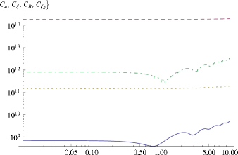
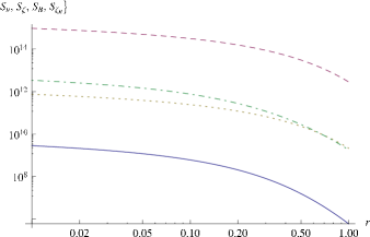
Figure 1: Temporal (left panel) and spatial (right panel) autocorrelations of velocity (solid line), vorticity (dashed line), magnetic field (dotted line) and magnetic vorticity (dot-dashed line), when $q=1.5$.

From Figure 1 it is evident that flows of above mentioned kind exhibit large temporal and spatial autocorrelations of perturbation and hence large energy dissipations of perturbation at least in the time and length scales of interest, leading to instability and plausible turbulence.

4 Summary and conclusions

In this work, we have attempted to address the origin of instability and then turbulence in magnetized, rotating, shear flows in presence of stochastic noise. Our particular emphasis is the flows having decreasing angular velocity but increasing specific angular momentum with the radial coordinate, which are Rayleigh stable. The flows with such a kind of velocity profile are often seen in astrophysics. As the molecular viscosity in astrophysical accretion disks is negligible, any transport of matter therein would arise through turbulence only, in order to explain observed data. In the cases of hot flows, e.g. disks around black holes, magnetorotational instability is generally believed to be responsible for turbulence and hence transport of angular momentum therein. However many authors argued for limitations of magnetorotational instability (Mahajan & Krishan (2008); Paoletti et al. (2012); Avila (2012)). Therefore, essentially we have addressed here the plausible origin of viscosity in rotating shear flows of the kind mentioned above.

References

- Avila (2012) Avila, M., Phys. Rev. Lett. 108, 124501 (2012) ApJ 629, 383 (2005).
- Barabási & Stanley (1995) Barabási, A.-L. & Stanley, H. E.,Fractal concepts in surface growth (Cambridge University Press, 1995)
- Chattopadhyay & Bhattacharjee (2000) Chattopadhyay, A. K., & Bhattacharjee, J. K., Phys. Rev. E 63, 016306 (2000)
- Forster, Nelson & Stephen (1977) Forster, D., Nelson, D. R., & Stephen, M. J., Phys. Rev. A 16, 732 (1977)
- Mahajan & Krishan (2008) Mahajan, S. M., & Krishan, V., ApJ 682, 602 (2008)
- Mukhopadhyay & Chattopadhyay (2013) Mukhopadhyay, B., & Chattopadhyay, A. K., J. Phys. A 46, 035501 (2013)
- Paoletti et al. (2012) Paoletti, M. S., van Gils, D. P. M., Dubrulle, B., Sun, C., Lohse, D., & Lathrop, D. P., A&A 547, A64 (2012)