Structure-Preserving Flows of Symplectic Matrix Pairs

Abstract

We construct a nonlinear differential equation of matrix pairs $(\mathcal{M}(t),\mathcal{L}(t))$ that is invariant (the Structure-Preserving Property) in the class of symplectic matrix pairs

$$\mathbb{S}_{\mathcal{S}_{1},\mathcal{S}_{2}}=\left\{\left(\mathcal{M},\mathcal{L}\right)|\ \mathcal{M}=\left[\begin{array}[]{cc}X_{12}&0\\ X_{22}&I\\ \end{array}\right]\mathcal{S}_{2},\ \ \mathcal{L}=\left[\begin{array}[]{cc}I&X_{11}\\ 0&X_{21}\\ \end{array}\right]\mathcal{S}_{1}\right.$$

$$\left.\text{ and }X=\left[\begin{array}[]{cc}X_{11}&X_{12}\\ X_{21}&X_{22}\\ \end{array}\right]\text{ is Hermitian}\right\}$$

for certain fixed symplectic matrices $\mathcal{S}_{1}$ and $\mathcal{S}_{2}$. Its solution also preserves invariant subspaces on the whole orbit (the Eigenvector-Preserving Property). Such a flow is called a structure-preserving flow and is governed by a Riccati differential equation (RDE) having the form

$$\begin{array}[]{l}\dot{W}(t)=[-W(t),I]\mathscr{H}[I,W(t)^{\top}]^{\top},\\ W(0)=W_{0},\end{array}$$

for some suitable Hamiltonian matrix $\mathscr{H}$. In addition, Radon’s lemma ([67] or see Theorem 3.8) leads to the explicit form $W(t)=P(t)Q(t)^{-1}$ where $[Q(t)^{\top},P(t)^{\top}]^{\top}=e^{\mathscr{H}t}[I,W_{0}^{\top}]^{\top}$. Therefore, blow-ups for the structure-preserving flows may happen at a finite $t$ whenever $Q(t)$ is singular. To continue, we then utilize the Grassmann manifolds to extend the domain of the structure-preserving flow to the whole $\mathbb{R}$ subtracting some isolated points.

On the other hand, the Structure-Preserving Doubling Algorithm (SDA) is an efficient numerical method for solving algebraic Riccati equations and nonlinear matrix equations. In conjunction with the structure-preserving flow, we consider the following two special classes of symplectic pairs: $\mathbb{S}_{1}=\mathbb{S}_{I_{2n},I_{2n}}$ and $\mathbb{S}_{2}=\mathbb{S}_{-I_{2n},\mathcal{J}}$ and the corresponding algorithms SDA-1 and SDA2. It is shown that at $t=2^{k-1},k\in\mathbb{Z}$ this flow passes through the iterates generated by SDA-1 and SDA-2, respectively. Therefore, the SDA and its corresponding structure-preserving flow have identical asymptotic behaviors, including the stability, instability, periodicity, and quasi-periodicity of the dynamics.

Taking advantage of the special structure and properties of the Hamiltonian matrix, we apply a symplectically similar transformation introduced by [58] to reduce $\mathscr{H}$ to a Hamiltonian Jordan canonical form $\mathfrak{J}$. The asymptotic analysis of the structure-preserving flows and RDEs is studied by using $e^{\mathfrak{J}t}$. The convergence of the SDA as well as its rate can thus result from the study of the structure-preserving flows. A complete asymptotic dynamics of the SDA is investigated, including the linear and quadratic convergence studied in the literature [12, 41, 46].

1 Introduction

We first introduce the algebraic structures that we consider in this paper. Let

$$\mathcal{J}_{n}=\left[\begin{array}[]{cc}0&I_{n}\\ -I_{n}&0\end{array}\right],$$

where $I_{n}$ is the $n\times n$ identity matrix. For convenience, we use $\mathcal{J}$ for $\mathcal{J}_{n}$ by dropping the subscript “$n$” if the order of $\mathcal{J}_{n}$ is clear in the context.

Definition 1.1.

• A matrix $\mathcal{H}\in\mathbb{C}^{2n\times 2n}$ is Hamiltonian if $\mathcal{H}\mathcal{J}=(\mathcal{H}\mathcal{J})^{H}$.

• A matrix pair $(\mathcal{M}_{h},\mathcal{L}_{h})$ with $\mathcal{M}_{h},\mathcal{L}_{h}\in\mathbb{C}^{2n\times 2n}$ is called a Hamiltonian pair if $\mathcal{M}_{h}\mathcal{J}\mathcal{L}_{h}^{H}=-\mathcal{L}_{h}\mathcal{J}\mathcal{M}_{h}^{H}$.

• A matrix $\mathcal{S}\in\mathbb{C}^{2n\times 2n}$ is symplectic if $\mathcal{S}\mathcal{J}\mathcal{S}^{H}=\mathcal{J}$.

• A matrix pair $(\mathcal{M}_{s},\mathcal{L}_{s})$ with $\mathcal{M}_{s},\mathcal{L}_{s}\in\mathbb{C}^{2n\times 2n}$ is called a symplectic pair if $\mathcal{M}_{s}\mathcal{J}\mathcal{M}_{s}^{H}=\mathcal{L}_{s}\mathcal{J}\mathcal{L}_{s}^{H}$.

Denote by $Sp(n)$ the multiplicative group of all $2n\times 2n$ symplectic matrices and by $\mathbb{H}(2n)$ the additive group of all $2n\times 2n$ Hermitian matrices. The matrix pairs $(A_{1},B_{1})$ and $(A_{2},B_{2})\in\mathbb{C}^{n\times n}\times\mathbb{C}^{n\times n}$ are said to be left equivalent, denoted by

$$(A_{1},B_{1})\overset{\textrm{l.e.}}{\sim}(A_{2},B_{2})$$

if $A_{1}=CA_{2}$, $B_{1}=CB_{2}$ for some invertible matrix $C$. A matrix pair $(A,B)$ is said to be regular if det$(A-\lambda B)\neq 0$ for some $\lambda\in\mathbb{C}$. It is well-known that for a regular matrix pair $(A,B)$ there are invertible matrices $P$ and $Q$ which transform $(A,B)$ to the Kronecker canonical form [34] as

$$PAQ=\left[\begin{array}[]{cc}J&0\\ 0&I\\ \end{array}\right],\ \ \ \ PBQ=\left[\begin{array}[]{cc}I&0\\ 0&N\\ \end{array}\right],$$

where $J$ is a Jordan matrix corresponding to the finite eigenvalues of $(A,B)$ and $N$ is a nilpotent Jordan matrix corresponding to the infinity eigenvalues. The index of a matrix pair $(A,B)$ is the index of nilpotency of $N$, i.e., the matrix pair $(A,B)$ is of index $\nu$, denoted by $\nu={\rm ind}_{\infty}(A,B)$, if $N^{\nu-1}\neq 0$ and $N^{\nu}=0$. By convention, if $B$ is invertible, the pair $(A,B)$ is said to be of index zero.

The following three types of Riccati-type equations appear in many fields of applied sciences.

• Continuous-time Algebraic Riccati Equation (CARE) [54, 62]:

  $$-XGX+A^{H}X+XA+H=0,$$ (1.1)

  where $A,H,G\in\mathbb{C}^{n\times n}$ with $G=G^{H}\geqslant 0$, $H=H^{H}\geqslant 0$ (positive semi-definite).

• Discrete-time Algebraic Riccati Equation (DARE) [54, 62]:

  $$X=A^{H}X(I+GX)^{-1}A+H,$$ (1.2)

  where $A,H,G\in\mathbb{C}^{n\times n}$ with $G=G^{H}\geqslant 0$, $H=H^{H}\geqslant 0$.

• Nonlinear Matrix Equation (NME) [27]:

  $$X+A^{H}X^{-1}A=Q,$$ (1.3)

  where $A,Q\in\mathbb{C}^{n\times n}$ with $Q=Q^{H}>0$.

These classical Riccati-type matrix equations occur in many important applications (see [3, 28, 54, 62] and references therein). The CAREs and DAREs have been studied extensively (see [2, 6, 7, 8, 14, 36, 37, 42, 48, 53, 54, 55, 61, 60, 62, 65, 70]). The NMEs have been studied in [3, 26, 28, 38]. The solutions of the Riccati-type equations can be solved by iterative methods such as the fixed-point iteration, the Newton’s method, and the Structure-Preserving Doubling Algorithms (SDAs) [27, 39, 54, 59, 62, 63]. Recently, SDAs for solving the stabilizing solutions of the three Riccati-type equations have been applied successfully in many industrial applications. For instance, in the vibration analysis of fast trains [41] and Green’s function calculation in nano research [40], $Q=Q^{T}$ and $A=A^{T}$ in (1.3) instead of being Hermitian. In the $\text{H}_{\infty}$- optimal controls [29, 62], the Riccati-type equations used are (1.1) and (1.2) but with $G$ and $H$ being Hermitian but not definite. Lack of positive semi-definiteness of $G$ and $H$ in general may cause possible breakdown in iteration formula containing an $(I+GH)^{-1}$ term such as the one in (1.8) below with $G=G_{k},H=H_{k}$, but in the above applications some extra physical properties were used to show that the breakdown would never happen. Since the SDAs developed in papers [27, 39, 54, 59, 62, 63] enjoy well-defined iterates and favorable convergence rates, it is tempting to design SDAs that can be applied to new Riccati-type matrix equations in which the matrices $G,H$ and $Q$ are just Hermitian. Indeed, we shall demonstrate that a class of SDAs can be designed to produce sequences of symplectic matrix pairs in special forms as in (1.14) below. Furthermore, their convergence behavior and general property can be studied by a related continuous dynamical system which is structure-preserving such that each symplectic pair generated by the SDA coincides with the solution of the structure-preserving flow at some time-step. We now describe these SDAs for solving DARE/CARE and NME with the matrices $G,H$ and $Q$ being Hermitian, not necessarily positive semi-definite.

• For solving DAREs (1.2), the symplectic pairs $(\mathcal{M}_{k},\mathcal{L}_{k})=\left(\left[\begin{array}[]{cc}A_{k}&0\\ -H_{k}&I\end{array}\right],\left[\begin{array}[]{cc}I&G_{k}\\ 0&A_{k}^{H}\end{array}\right]\right)$ are generated by

  • Algorithm SDA-1.

    $$\begin{array}[]{l}A_{0}=A,~{}G_{0}=G,~{}H_{0}=H,\\ A_{k+1}=A_{k}(I+G_{k}H_{k})^{-1}A_{k},\\ G_{k+1}=G_{k}+A_{k}G_{k}(I+H_{k}G_{k})^{-1}A_{k}^{H},\\ H_{k+1}=H_{k}+A_{k}^{H}(I+H_{k}G_{k})^{-1}H_{k}A_{k}.\end{array}$$ (1.8)

  It has been shown in [46, 59] that under some mild conditions, the sequence of symplectic pairs $(\mathcal{M}_{k},\mathcal{L}_{k})$ quadratically/linearly converges, in which, as $k\to\infty$

  $$H_{k}\to\text{ the stabilizing solution of \eqref{eq1.2}},$$

  $$G_{k}\to\text{ the stabilizing solution of the dual equation of \eqref{eq1.2}},$$

  $$A_{k}\to 0.$$

  Here the dual equation of (1.2) is of the form

  $$Y=AY(I+HY)^{-1}A^{H}+G.$$

• For solving CAREs (1.1), one can transform it into a DARE (1.2) by using a suitable Cayley transformation [64]. Then Algorithm SDA-1 can be employed to find the desired stabilizing solution of CAREs.

• For solving NMEs (1.3), the symplectic pairs $(\mathcal{M}_{k},\mathcal{L}_{k})=\left(\left[\begin{array}[]{cc}A_{k}&0\\ Q_{k}&-I\end{array}\right],\left[\begin{array}[]{cc}-P_{k}&I\\ A^{H}_{k}&0\end{array}\right]\right)$ are generated by

  • Algorithm SDA-2.

    $$\begin{array}[]{l}A_{0}=A,~{}Q_{0}=Q,~{}P_{0}=0,\\ A_{k+1}=A_{k}(Q_{k}-P_{k})^{-1}A_{k},\\ Q_{k+1}=Q_{k}-A_{k}^{H}(Q_{k}-P_{k})^{-1}A_{k},\\ P_{k+1}=P_{k}+A_{k}(Q_{k}-P_{k})^{-1}A_{k}^{H}.\end{array}$$ (1.13)

  It has been shown in [12, 59] that under some conditions, the sequence of symplectic pairs $(\mathcal{M}_{k},\mathcal{L}_{k})$ quadratically/linearly converges, in which, as $k\to\infty$

  $$Q_{k}\to\text{ the maximal solution of \eqref{eq1.3}},$$

  $$P_{k}\to\text{ the minimal solution of \eqref{eq1.3}},$$

  $$A_{k}\to 0.$$

Eigenvector-Preserving Property:

For each case above, if $\mathcal{M}_{k}U=\mathcal{L}_{k}US$ or $\mathcal{M}_{k}VT=\mathcal{L}_{k}V$, where $U,V\in\mathbb{C}^{2n\times r}$ and $S,T\in\mathbb{C}^{r\times r}$, then $\mathcal{M}_{k+1}U=\mathcal{L}_{k+1}US^{2}$ or $\mathcal{M}_{k+1}VT^{2}=\mathcal{L}_{k+1}V$, i.e., the SDA preserves the invariant subspaces for each $k$ and the squares of eigenvalues;

Structure-Preserving Property:

The sequences of symplectic pairs $\{(\mathcal{M}_{k},\mathcal{L}_{k})\}_{k=1}^{\infty}$ generated by Algorithms SDA-1 and SDA-2 are, respectively, invariant in the sets

$$\mathbb{S}_{1}=\left\{\left(\left[\begin{array}[]{cc}A&0\\ H&I\\ \end{array}\right],\left[\begin{array}[]{cc}I&G\\ 0&A^{H}\\ \end{array}\right]\right)\ |\ A,\ H=H^{H},\ G=G^{H}\in\mathbb{C}^{n\times n}\right\},$$ (1.14e)

and

$$\mathbb{S}_{2}=\left\{\left(\left[\begin{array}[]{cc}A&0\\ Q&-I\\ \end{array}\right],\left[\begin{array}[]{cc}P&I\\ A^{H}&0\\ \end{array}\right]\right)\ |\ A,\ Q=Q^{H},\ P=P^{H}\in\mathbb{C}^{n\times n}\right\}.$$ (1.14j)

To study the symplectic pairs, we first quote the following theorem in [63] regarding a simple left equivalence for regular symplectic pairs.

Theorem 1.1.

(see [63]) Let $(\mathcal{M},\mathcal{L})$ be a regular symplectic pair with $\mathcal{M},\ \mathcal{L}\in\mathbb{C}^{2n\times 2n}$. Then there exist $\mathcal{S}_{1}$, $\mathcal{S}_{2}\in Sp(n)$ and a Hermitian matrix $X=\left[\begin{array}[]{cc}X_{11}&X_{12}\\ X_{21}&X_{22}\\ \end{array}\right]$ such that

$$(\mathcal{M},\mathcal{L})\overset{\rm{l.e.}}{\sim}\left(\left[\begin{array}[]{cc}X_{12}&0\\ X_{22}&I\\ \end{array}\right]\mathcal{S}_{2},\left[\begin{array}[]{cc}I&X_{11}\\ 0&X_{21}\\ \end{array}\right]\mathcal{S}_{1}\right).$$

Theorem 1.1 provides us a classification for symplectic pairs. Specifically, let $\mathcal{S}_{1},\mathcal{S}_{2}\in Sp(n)$. We denote the class of symplectic pairs generated by $\mathcal{S}_{1},\mathcal{S}_{2}$ as

$$\mathbb{S}_{\mathcal{S}_{1},\mathcal{S}_{2}}=\left\{\left(\mathcal{M},\mathcal{L}\right)|\ \mathcal{M}=\left[\begin{array}[]{cc}X_{12}&0\\ X_{22}&I\\ \end{array}\right]\mathcal{S}_{2},\ \ \mathcal{L}=\left[\begin{array}[]{cc}I&X_{11}\\ 0&X_{21}\\ \end{array}\right]\mathcal{S}_{1}\right.$$ (1.15e)

$$\left.\text{ and }X=\left[\begin{array}[]{cc}X_{11}&X_{12}\\ X_{21}&X_{22}\\ \end{array}\right]\in\mathbb{H}(2n)\right\}.$$ (1.15h)

It is easily seen that each pair $$(\mathcal{M},\mathcal{L})\in\mathbb{S}_{\mathcal{S}_{1},\mathcal{S}_{2}} \mathbb{H}(2n) \mathbb{S}_{\mathcal{S}_{1},\mathcal{S}_{2}} T_{\mathcal{S}_{1},\mathcal{S}_{2}}:\mathbb{H}(2n)\to\mathbb{S}_{\mathcal{S}_{1},\mathcal{S}_{2}}$$ is symplectic. The bijective correspondence between and can be constructed by the transformation with

$$T_{\mathcal{S}_{1},\mathcal{S}_{2}}(X)=\left(\left[\begin{array}[]{cc}X_{12}&0\\ X_{22}&I\\ \end{array}\right]\mathcal{S}_{2},\left[\begin{array}[]{cc}I&X_{11}\\ 0&X_{21}\\ \end{array}\right]\mathcal{S}_{1}\right).$$ (1.15m)

Therefore, the invariant sets for SDA-1 and SDA-2, i.e., $\mathbb{S}_{1}$ and $\mathbb{S}_{2}$, respectively, given in (1.14), can be rewritten as $\mathbb{S}_{1}=\mathbb{S}_{I_{2n},I_{2n}}$ and $\mathbb{S}_{2}=\mathbb{S}_{-I_{2n},\mathcal{J}}$. Note that $\mathbb{S}_{1}\nsubseteq\mathbb{S}_{2}$, $\mathbb{S}_{2}\nsubseteq\mathbb{S}_{1}$. In [49], a parameterized curve is constructed in $\mathbb{S}_{2}$ passing through the iterates generated by the fixed-point iteration, the SDA and the Newton’s method with some additional conditions. Finding a smooth curve with a specific structure that passes through a sequence of iterates generated by some numerical algorithm is a popular topic studied by many researchers, especially in the study of the so-called Toda flow that links matrices/matrix pairs generated by QR/QZ-algorithm [15, 16, 17, 18, 19, 69]. The Toda flow is the solution of a nonlinear ordinary differential matrix equation in which the eigenvalues are preserved, but the eigenvectors are changed in $t$. Rather than the invariance property of Toda flows, in this paper we shall focus on the flows $(\mathcal{M}(t),\mathcal{L}(t))$ on a specified $\mathbb{S}_{\mathcal{S}_{1},\mathcal{S}_{2}}$ (i.e., the Structure-Preserving Property) that has Eigenvector-Preserving Property. More precisely, for a flow $\{(\mathcal{M}(t),\mathcal{L}(t))\ |\ t\in\mathbb{R}\}\subseteq\mathbb{S}_{\mathcal{S}_{1},\mathcal{S}_{2}}$ satisfying the initial value problem with an initial regular pair $(\mathcal{M}(1),\mathcal{L}(1))=(\mathcal{M}_{1},\mathcal{L}_{1})$, the Eigenvector-Preserving Property of this flow can be stated as follows:

• Assume that

  $$\mathcal{M}_{1}U_{0}=0,\ \ \mathcal{L}_{1}U_{\infty}=0,\ \ \mathcal{M}_{1}U_{1}=\mathcal{L}_{1}U_{1}S,\ \ \mathcal{M}_{1}V_{1}T=\mathcal{L}_{1}V_{1},$$ (1.16)

  where $[U_{0},U_{\infty},U_{1},V_{1}]\in\mathbb{C}^{2n\times 2n}$ is invertible, and $S$ and $T$ have no semi-simple zero eigenvalues. Then

  $$\mathcal{M}(t)U_{0}=0,\ \ \mathcal{L}(t)U_{\infty}=0,\ \ \mathcal{M}(t)U_{1}=\mathcal{L}(t)U_{1}S^{t},\ \ \mathcal{M}(t)V_{1}T^{t}=\mathcal{L}(t)V_{1}$$ (1.17)

  hold.

Here in (1.17), $S^{t}$ and $T^{t}$, for $t\in\mathbb{R}$, represent the matrix exponentials. Because $z^{t}=\exp(t\log(z))$ for each $z\in\mathbb{C}\setminus\{0\}$, it follows from [43, Definition 1.11 and Theorem 1.17] that the matrix exponentials $S^{t}$ and $T^{t}$ are well-defined if $S$ and $T$ are invertible. On the other hand, if $S$ (or $T$) is singular, then $S^{t}$ (or $T^{t}$) for $t\in\mathbb{R}$ is undefined. Hence, to make the Eigenvector-Preserving Property meaningful, we assume that the matrices $S$ and $T$ in (1.16) are invertible. This coincides with the assumption that the regular symplectic pair $(\mathcal{M}_{1},\mathcal{L}_{1})$ has only semi-simple zero and infinite eigenvalues (if exists). We shall show in Theorem 2.3 that this assumption for $(\mathcal{M}_{1},\mathcal{L}_{1})$ can result from the condition ${\rm ind}_{\infty}(\mathcal{M}_{1},\mathcal{L}_{1})\leqslant 1$. Throughout this paper, we assume that the initial matrix pair $(\mathcal{M}_{1},\mathcal{L}_{1})$ is regular and symplectic with ${\rm ind}_{\infty}(\mathcal{M}_{1},\mathcal{L}_{1})\leqslant 1$. Note that if a matrix pair $(A,B)$ is regular and of index at most one, the corresponding time-invariant continuous system

$$B\frac{dx}{dt}=Ax(t)+f(t)$$

has a unique solution for all admissible $f(t)$ with consistent initial conditions [35, 62]. However, if the index of $(A,B)$ is larger than one, impulses can occur in the time-invariant continuous system [35].

This paper is organized as follows. In Section 2, we introduce some preliminary results. In Sections 3, we construct a differential equation such that its solution is invariant in $\mathbb{S}_{\mathcal{S}_{1},\mathcal{S}_{2}}$ and has Eigenvector-Preserving Property for certain fixed symplectic matrices $\mathcal{S}_{1}$, $\mathcal{S}_{2}$. Such a flow is called a structure-preserving flow. On the other hand, we also study the algebraic equation that is determined by both the Eigenvector-Preserving Property and the Structure-Preserving Property, in which the solution curve is denoted by $\mathcal{C}_{\mathcal{M}_{1},\mathcal{L}_{1}}$. We further show that the phase portrait of the structure-preserving flow is $\mathcal{C}_{\mathcal{M}_{1},\mathcal{L}_{1}}$. In Subsection 3.2, it will be shown that structure-preserving flows are governed by the Riccati differential equations (RDE) of the form

$$\begin{array}[]{l}\dot{W}(t)=[-W(t),I]\mathscr{H}[I,W(t)^{\top}]^{\top},\\ W(0)=W_{0},\end{array}$$

where $\mathscr{H}$ is a suitable Hamiltonian matrix. In addition, Radon’s lemma ([67] or see Theorem 3.8) leads to the explicit form $W(t)=P(t)Q(t)^{-1}$, where $[Q(t)^{\top},P(t)^{\top}]^{\top}=e^{\mathscr{H}t}[I,W_{0}^{\top}]^{\top}$. This important relationship between linear differential equations and Riccati differential equations will be used to obtain an explicit representation formula for all solutions of RDEs as well as the structure-preserving flows. Therefore, the blow-up can occur at some finite time $t$ whenever $Q(t)$ is singular. In Subsection 3.3, we adopt the Grassmann manifold to extend the domain of the structure-preserving flow to the whole $\mathbb{R}$ except some isolated points. For two special classes of symplectic pairs $\mathbb{S}_{1}=\mathbb{S}_{I_{2n},I_{2n}}$ and $\mathbb{S}_{2}=\mathbb{S}_{-I_{2n},\mathcal{J}}$, it is shown in Subsection 3.4 that the structure-preserving flow passes through the iterates generated by SDA-1 and SDA-2, respectively. Therefore, the SDA and its associated structure-preserving flow have identical asymptotic behaviors, including the stability, instability, periodicity, and quasi-periodicity of the dynamics. In Section 4, we investigate the asymptotic behavior of $[Q(t)^{\top},P(t)^{\top}]^{\top}$ and use the results to analyze the convergence of SDAs. Due to the special structure and properties of the Hamiltonian matrix, we apply a symplectic similarity transformation introduced by [58] to reduce $\mathscr{H}$ to a Hamiltonian Jordan canonical form $\mathfrak{J}$. In Subsections 4.1 and 4.2, we first study the structure of $e^{\mathfrak{J}t}$ and then the asymptotic behaviors of $W(t)$ and $Q(t)^{-1}$, as $t\to\pm\infty$, with $\mathfrak{J}$ being of elementary cases. The results for general $\mathfrak{J}$ are given in Subsection 4.3. The asymptotic analysis of SDAs as well as its convergence rate by using the asymptotic behavior of RDEs are shown in Subsection 4.4. Complementary proofs in Sections 2 and 4 are given in Appendix.

2 Preliminaries

In this section, we introduce notation, definitions and some preliminary results. For a matrix $A\in\mathbb{C}^{n\times n}$, $A^{H}$ and $A^{\top}$ are the conjugate transpose and the transpose of $A$, respectively. $\sigma(A)$ denotes the spectrum of $A$. For each $\lambda_{0}\in\sigma(A)$, $\mathcal{R}_{\lambda_{0}}(A)=\{x|(A-\lambda_{0}I)^{\nu}x=0\text{ for some }\nu\in\mathbb{N}\}$ is the generalized eigenspace of $A$ corresponding to the eigenvalue $\lambda_{0}$. For a regular matrix pair $(A,B)$ with $A,B\in\mathbb{C}^{n\times n}$, $\sigma(A,B)$ denotes the spectrum of $(A,B)$. Note that the matrix pair $(A,B)$ is said to have eigenvalues at infinity if $B$ is singular.

Definition 2.1.

Two subspaces $\mathbb{U}$ and $\mathbb{V}$ of $\mathbb{C}^{2n}$ are called $\mathcal{J}$-orthogonal if $u^{H}\mathcal{J}v=0$ for each $u\in\mathbb{U}$ and $v\in\mathbb{V}$. A subspace $\mathbb{U}$ of $\mathbb{C}^{2n}$ is called isotropic if $x^{H}\mathcal{J}y=0$ for any $x,y\in\mathbb{U}$. An $n$-dimensional isotropic subspace is called a Lagrangian subspace.

Suppose that $\mathcal{H}\in\mathbb{C}^{n\times n}$ is Hamiltonian. It is well-known that for $\lambda,\mu\in\sigma(\mathcal{H})$ with $\lambda\neq-\bar{\mu}$, the subspaces $\mathcal{R}_{\lambda}(\mathcal{H})$ and $\mathcal{R}_{\mu}(\mathcal{H})$ are $\mathcal{J}$-orthogonal. Similarly, for a symplectic matrix $\mathcal{S}\in Sp(n)$ and $\lambda,\mu\in\sigma(\mathcal{S})$ with $\lambda\neq 1/\bar{\mu}$, $\mathcal{R}_{\lambda}(\mathcal{S})$ and $\mathcal{R}_{\mu}(\mathcal{S})$ are $\mathcal{J}$-orthogonal. The $\mathcal{J}$-orthogonality also holds for invariant subspaces of Hamiltonian pairs and symplectic pairs. To prove this, we need the following lemma.

Lemma 2.1.

Suppose that $(A_{1},B_{1})$ and $(A_{2},B_{2})\in\mathbb{C}^{n\times n}\times\mathbb{C}^{n\times n}$ are regular matrix pairs. If $\sigma(A_{1},B_{1})\cap\sigma(-A_{2},B_{2})=\emptyset$, then the equation

$$A_{2}XB_{1}+B_{2}XA_{1}=0$$ (2.1)

has only trivial solution.

Proof.

We first consider the case that both $B_{1}$ and $B_{2}$ are invertible. Since $\sigma(B_{1}^{-1}A_{1})\cap\sigma(-B_{2}^{-1}A_{2})=\sigma(A_{1},B_{1})\cap\sigma(-A_{2},B_{2})=\emptyset$, Eq. (2.1) has only trivial solution.

For the general case, we may assume that $B_{1}$ is singular. Therefore $(A_{1},B_{1})$ has eigenvalues at infinity. Since $\sigma(A_{1},B_{1})\cap\sigma(-A_{2},B_{2})=\emptyset$, $B_{2}$ must be nonsingular. Let $\widehat{A}_{2}=B_{2}^{-1}A_{2}$. Since $(A_{1},B_{1})$ is regular, there are nonsingular matrices $P$ and $Q$ such that

$$PA_{1}Q=\left[\begin{array}[]{cc}J_{1}&0\\ 0&I\\ \end{array}\right],\ \ \ \ PB_{1}Q=\left[\begin{array}[]{cc}I&0\\ 0&N_{1}\\ \end{array}\right],$$

where $N_{1}$ is nilpotent. Then (2.1) can be transformed into

$$\begin{array}[]{l}\widehat{A}_{2}\widehat{X}_{1}+\widehat{X}_{1}J_{1}=0,\\ \widehat{A}_{2}\widehat{X}_{2}N_{1}+\widehat{X}_{2}=0,\end{array}$$

where $[\widehat{X}_{1},\widehat{X}_{2}]:=XP^{-1}$. Since $\sigma(\widehat{A}_{2})\cap\sigma(-J_{1})=\emptyset$ and $\sigma(N_{1}^{\top}\otimes\widehat{A}_{2})=\{0\}$, we have $\widehat{X}_{1}=0$ and $\widehat{X}_{2}=0$, then $X=[\widehat{X}_{1},\widehat{X}_{2}]P=0$. Hence, Eq. (2.1) has only trivial solution. ∎

Theorem 2.2.

Let $(\mathcal{M},\mathcal{L})$, $(R_{1},T_{1})$ and $(R_{2},T_{2})$ be regular pairs and $U_{1}$ and $U_{2}$ be of full column rank satisfying

$$\mathcal{M}U_{1}T_{1}=\mathcal{L}U_{1}R_{1},\text{ and }\mathcal{M}U_{2}T_{2}=\mathcal{L}U_{2}R_{2}.$$ (2.2)

• If $(\mathcal{M},\mathcal{L})$ is Hamiltonian and $\sigma(R_{1},T_{1})\cap\sigma(-R^{H}_{2},T^{H}_{2})=\emptyset$, then $U_{1}$ and $U_{2}$ are $\mathcal{J}$-orthogonal.

• If $(\mathcal{M},\mathcal{L})$ is symplectic and $\sigma(R_{1},T_{1})\cap\sigma(T^{H}_{2},R^{H}_{2})=\emptyset$, then $U_{1}$ and $U_{2}$ are $\mathcal{J}$-orthogonal.

Proof.

$(i)$ Since $(\mathcal{M},\mathcal{L})$ is a regular Hamiltonian pair, we have

$$\left[\mathcal{M}\mathcal{J},\mathcal{L}\right]\left[\begin{array}[]{c}\mathcal{L}^{H}\\ \mathcal{J}\mathcal{M}^{H}\\ \end{array}\right]=0,$$

and rank$[\mathcal{M}\mathcal{J},\mathcal{L}]=2n$. Hence, the column vectors of $\left[\begin{array}[]{c}\mathcal{L}^{H}\\ \mathcal{J}\mathcal{M}^{H}\\ \end{array}\right]$ form a basis of null space of $[\mathcal{M}\mathcal{J},\mathcal{L}]$. On the other hand, it follows from (2.2) that

$$\left[\mathcal{M}\mathcal{J},\mathcal{L}\right]\left[\begin{array}[]{c}\mathcal{J}^{H}U_{1}T_{1}\\ -U_{1}R_{1}\\ \end{array}\right]=0,$$ (2.5)

$$\left[R_{2}^{H}U_{2}^{H},-T_{2}^{H}U_{2}^{H}\mathcal{J}^{H}\right]\left[\begin{array}[]{c}\mathcal{L}^{H}\\ \mathcal{J}\mathcal{M}^{H}\\ \end{array}\right]=0.$$ (2.8)

Therefore, by (2.5) there is a nonsingular matrix $W$ such that

$$\left[\begin{array}[]{c}\mathcal{L}^{H}\\ \mathcal{J}\mathcal{M}^{H}\\ \end{array}\right]W=\left[\begin{array}[]{c}\mathcal{J}^{H}U_{1}T_{1}\\ -U_{1}R_{1}\\ \end{array}\right].$$

Multiplying $W$ from the right of (2.8), we have

$$0 =\left[R_{2}^{H}U_{2}^{H},-T_{2}^{H}U_{2}^{H}\mathcal{J}^{H}\right]\left[\begin{array}[]{c}\mathcal{J}^{H}U_{1}T_{1}\\ -U_{1}R_{1}\\ \end{array}\right]$$

$$=R_{2}^{H}(U_{2}^{H}\mathcal{J}^{H}U_{1})T_{1}+T_{2}^{H}(U_{2}^{H}\mathcal{J}^{H}U_{1})R_{1}.$$

Since $\sigma(R_{1},T_{1})\cap\sigma(-R^{H}_{2},T^{H}_{2})=\emptyset$, it follows from Lemma 2.1 that $U_{2}^{H}\mathcal{J}U_{1}=0$.

$(ii)$ Similarly, if $(\mathcal{M},\mathcal{L})$ is a regular symplectic pair, then from equations of (2.2) we have

$$T_{2}^{H}(U_{2}^{H}\mathcal{J}U_{1})T_{1}-R_{2}^{H}(U_{2}^{H}\mathcal{J}U_{1})R_{1}=0.$$

Since $\sigma(R_{1},T_{1})\cap\sigma(T^{H}_{2},R^{H}_{2})=\emptyset$, it follows from Lemma 2.1 that $U_{2}^{H}\mathcal{J}U_{1}=0$. ∎

From now on, we assume that the condition ${\rm ind}_{\infty}(\mathcal{M},\mathcal{L})\leqslant 1$ holds for a regular symplectic pair $(\mathcal{M},\mathcal{L})$, i.e., either the matrix pair $(\mathcal{M},\mathcal{L})$ has no eigenvalue at infinity or the Jordan block corresponding to the eigenvalues at infinity is a zero matrix.

Theorem 2.3.

Suppose $(\mathcal{M},\mathcal{L})$ is a regular symplectic pair with $\mathcal{M},\mathcal{L}\in\mathbb{C}^{2n\times 2n}$ and ${\rm ind}_{\infty}(\mathcal{M},\mathcal{L})\leqslant 1$. Then there is $\hat{n}\leqslant n$ such that ${\rm rank}(\mathcal{M})={\rm rank}(\mathcal{L})=n+\hat{n}$. In addition, there exist $U_{0},U_{\infty}\in\mathbb{C}^{2n\times\ell}$, $U_{1}\in\mathbb{C}^{2n\times 2\hat{n}}$ with $\ell=n-\hat{n}$ and a symplectic matrix $\widehat{\mathcal{S}}\in\mathbb{C}^{2\hat{n}\times 2\hat{n}}$ such that

$$\mathbf{U}^{H}\mathcal{J}_{n}\mathbf{U}=\left[\begin{array}[]{c|c}\mathcal{J}_{\hat{n}}&0\\ \hline\cr 0&\mathcal{J}_{\ell}\\ \end{array}\right]$$ (2.11)

with $\mathbf{U}=[U_{1}|U_{0},U_{\infty}]$, and

$$\mathcal{M}U_{0}=0,\ \ \mathcal{L}U_{\infty}=0,\ \ \mathcal{M}U_{1}=\mathcal{L}U_{1}\widehat{\mathcal{S}}.$$ (2.12)

Remark 2.1.

From (2.11), it is easily seen that $\mathbf{U}^{-1}=(\mathcal{J}_{\hat{n}}\oplus\mathcal{J}_{\ell})^{H}\mathbf{U}^{H}\mathcal{J}$.

Proof of Theorem 2.3.

From Theorem 1.1, the pair $(\mathcal{M},\mathcal{L})$ is left equivalent to the pair of the form $\left(\left[\begin{array}[]{cc}X_{12}&0\\ X_{22}&I\\ \end{array}\right]\mathcal{S}_{2},\left[\begin{array}[]{cc}I&X_{11}\\ 0&X_{21}\\ \end{array}\right]\mathcal{S}_{1}\right)$ for some $X=[X_{ij}]_{1\leq i,j\leq 2}\in\mathbb{H}(2n)$ and $\mathcal{S}_{1}$, $\mathcal{S}_{2}\in Sp(n)$. Therefore, the relation $X_{12}^{H}=X_{21}$, and the nonsingularity of $\mathcal{S}_{1}$ and $\mathcal{S}_{2}$ imply that ${\rm rank}(\mathcal{M})={\rm rank}(\mathcal{L})$. Since ${\rm ind}_{\infty}(\mathcal{M},\mathcal{L})\leqslant 1$, there exist $U_{0},U_{\infty}\in\mathbb{C}^{2n\times\ell}$ and $U_{1}\in\mathbb{C}^{2n\times 2(n-\ell)}$ such that the invariances of (2.12) hold, where $\widehat{\mathcal{S}}\in\mathbb{C}^{2(n-\ell)\times 2(n-\ell)}$ is nonsingular and the column spaces spanned by $U_{0}$, $U_{\infty}$ and $U_{1}$ are the eigenspaces of $(\mathcal{M},\mathcal{L})$ corresponding to zero, infinity and finite-nonzero eigenvalues, respectively. Applying Theorem 2.2(ii) by setting $T_{1}=T_{2}=I$, $R_{1}=R_{2}=0$ and $U_{1}=U_{2}=U_{0}$, respectively, we have $U_{0}^{H}\mathcal{J}_{n}U_{0}=0$. Similarly, $U_{1}^{H}\mathcal{J}_{n}U_{0}$, $U_{1}^{H}\mathcal{J}_{n}U_{\infty}$ and $U_{\infty}^{H}\mathcal{J}_{n}U_{\infty}$ are also zero matrices. In addition, noting that $\mathbf{U}$ is nonsingular, we have

$$[U_{1}|U_{0},U_{\infty}]^{H}\mathcal{J}_{n}[U_{1}|U_{0},U_{\infty}]=\left[\begin{array}[]{c|cc}K_{1}&0&0\\ \hline\cr 0&0&K_{2}\\ 0&-K_{2}^{H}&0\end{array}\right],$$ (2.16)

where $K_{1}$ is nonsingular skew-Hermitian and $K_{2}$ is nonsingular. Resetting $U_{\infty}:=U_{\infty}K_{2}^{-1}$, we then have $\mathcal{L}U_{\infty}=0$ and $[U_{0},U_{\infty}]^{H}\mathcal{J}_{n}[U_{0},U_{\infty}]=\mathcal{J}_{\ell}$. From the congruence transformation of (2.16), it is easily seen that Hermitian matrices $iK_{1}$ and $i\mathcal{J}_{\hat{n}}$ have the same inertia. Hence, there exists an invertible matrix $W$ such that $W^{H}K_{1}W=\mathcal{J}_{\hat{n}}$. Resetting $U_{1}:=U_{1}W$ and $\widehat{\mathcal{S}}:=W^{-1}\widehat{\mathcal{S}}W$, we then have $\mathcal{M}U_{1}=\mathcal{L}U_{1}\widehat{\mathcal{S}}$ and (2.11).

Now, we show that $\widehat{\mathcal{S}}$ is symplectic. Since $(\mathcal{M},\mathcal{L})$ is a regular symplectic pair, as in the proof of Theorem 2.2 above, the columns of $\left[\begin{array}[]{c}\mathcal{J}\mathcal{M}^{H}\\ -\mathcal{J}\mathcal{L}^{H}\\ \end{array}\right]$ form a basis of null space of $[\mathcal{M},\mathcal{L}]$. From (2.12), we have $\left[\mathcal{M},\mathcal{L}\right]\left[\begin{array}[]{c}U_{1}\\ -U_{1}\widehat{\mathcal{S}}\\ \end{array}\right]=0$. Hence there is a matrix $W\in\mathbb{C}^{2n\times 2\hat{n}}$ of full column rank such that

$$\left[\begin{array}[]{c}\mathcal{J}\mathcal{M}^{H}\\ -\mathcal{J}\mathcal{L}^{H}\\ \end{array}\right]W=\left[\begin{array}[]{c}U_{1}\\ -U_{1}\widehat{\mathcal{S}}\\ \end{array}\right].$$ (2.21)

Taking the conjugate transpose of (2.12), we obtain

$$0=\left[U_{1}^{H},-\widehat{\mathcal{S}}^{H}U_{1}^{H}\right]\left[\begin{array}[]{c}\mathcal{M}^{H}\\ \mathcal{L}^{H}\\ \end{array}\right]=\left[-U_{1}^{H}\mathcal{J},-\widehat{\mathcal{S}}^{H}U_{1}^{H}\mathcal{J}\right]\left[\begin{array}[]{c}\mathcal{J}\mathcal{M}^{H}\\ -\mathcal{J}\mathcal{L}^{H}\\ \end{array}\right].$$

Applying (2.11) and (2.21) to the last equation yields that

$$-\mathcal{J}_{\hat{n}}+\widehat{\mathcal{S}}^{H}\mathcal{J}_{\hat{n}}\widehat{\mathcal{S}}=\left[-U_{1}^{H}\mathcal{J},-\widehat{\mathcal{S}}^{H}U_{1}^{H}\mathcal{J}\right]\left[\begin{array}[]{c}U_{1}\\ -U_{1}\widehat{\mathcal{S}}\\ \end{array}\right]=0.$$

Thus, $\widehat{\mathcal{S}}$ is a symplectic matrix. ∎

Note that the matrix $\widehat{\mathcal{S}}$ in Theorem 2.3 is symplectic. It is proven in Theorem A.1 that there is a Hamiltonian matrix $\widehat{\mathcal{H}}$ satisfying $e^{\widehat{\mathcal{H}}}=\widehat{\mathcal{S}}$. Using $\widehat{\mathcal{H}}$, we shall construct a Hamiltonian matrix $\mathcal{H}$ which has invariant subspaces spanned by $U_{0}$, $U_{\infty}$, and $U_{1}$.

Theorem 2.4.

Suppose $(\mathcal{M},\mathcal{L})$ is a regular symplectic pair with $\mathcal{M},\mathcal{L}\in{\mathbb{C}}^{2n\times 2n}$ and ${\rm ind}_{\infty}(\mathcal{M},\mathcal{L})\leqslant 1$. Let the matrices $\mathbf{U}$ and $\widehat{\mathcal{S}}$ be given as in Theorem 2.3, and $\widehat{\mathcal{H}}\in\mathbb{C}^{2\hat{n}\times 2\hat{n}}$ be the Hamiltonian matrix such that

$$e^{\widehat{\mathcal{H}}}=\widehat{\mathcal{S}}.$$ (2.22)

Then the matrix

$$\mathcal{H}=\mathbf{U}\left[\begin{array}[]{cc}\widehat{\mathcal{H}}&0\\ 0&0\\ \end{array}\right](\mathcal{J}_{\hat{n}}\oplus\mathcal{J}_{\ell})^{H}\mathbf{U}^{H}\mathcal{J}$$ (2.25)

is Hamiltonian.

Proof.

Since $\widehat{\mathcal{H}}$ is Hamiltonian, we have

$$\mathcal{H}\mathcal{J} =-\mathbf{U}\left[\begin{array}[]{cc}\widehat{\mathcal{H}}\mathcal{J}_{\hat{n}}^{H}&0\\ 0&0\\ \end{array}\right]\mathbf{U}^{H}=-\mathbf{U}\left[\begin{array}[]{cc}\mathcal{J}_{\hat{n}}\widehat{\mathcal{H}}^{H}&0\\ 0&0\\ \end{array}\right]\mathbf{U}^{H}$$

$$=\mathcal{J}^{H}\mathcal{J}^{H}\mathbf{U}\left[\begin{array}[]{cc}\mathcal{J}_{\hat{n}}\widehat{\mathcal{H}}^{H}&0\\ 0&0\\ \end{array}\right]\mathbf{U}^{H}=\mathcal{J}^{H}\mathcal{H}^{H}.$$

Hence, $\mathcal{H}$ is Hamiltonian. ∎

Remark 2.2.

Suppose that $(\mathcal{M},\mathcal{L})$ is a real regular symplectic pair. Then $\mathbf{U}$ is real and $\widehat{\mathcal{S}}$ is real symplectic. In [23], under the assumptions

• $\widehat{\mathcal{S}}$ has an even number of Jordan blocks of each size relative to every negative eigenvalue;

• the size of two identical Jordan blocks corresponding to eigenvalue $-1$ is odd;

it is shown that there is a real Hamiltonian matrix $\widehat{\mathcal{H}}$ such that $e^{\widehat{\mathcal{H}}}=\widehat{\mathcal{S}}$. Hence, the Hamiltonian $\mathcal{H}$ defined in (2.25) is real.

Suppose that $\mathcal{L}$ is invertible. It follows from Theorem 2.3 that $\mathcal{M}$ is also invertible. Therefore, $U_{0}$ and $U_{\infty}$ in (2.12) are absent. On the other hand, the matrix $\mathcal{L}^{-1}\mathcal{M}$ is symplectic. From (2.12) and Theorem 2.4, we have that $e^{\mathcal{H}}=\mathcal{L}^{-1}\mathcal{M}$ for some Hamiltonian matrix $\mathcal{H}$, that is, $\mathcal{M}=\mathcal{L}e^{\mathcal{H}}$. For the case that $\mathcal{L}$ is singular and $(\mathcal{M},\mathcal{L})$ is a regular symplectic pair with ${\rm ind}_{\infty}(\mathcal{M},\mathcal{L})\leqslant 1$, it is natural to ask whether there is a Hamiltonian matrix $\mathcal{H}$ such that $\mathcal{M}=\mathcal{L}e^{\mathcal{H}}$. To this end, we need the following lemma.

Lemma 2.5.

Suppose that $(\mathcal{M},\mathcal{L})$ is a regular symplectic pair. If $\mathcal{M}=\mathcal{L}W$ for some nonsingular $W$, then both $\mathcal{M}$ and $\mathcal{L}$ are invertible.

Proof.

From Theorem 1.1, there are two symplectic matrices $\mathcal{S}_{1}$ and $\mathcal{S}_{2}$, and a Hermitian matrix $X=[X_{ij}]_{1\leq i,j\leq 2}$ such that

$$\mathcal{M}=C\left[\begin{array}[]{cc}X_{12}&0\\ X_{22}&I\\ \end{array}\right]\mathcal{S}_{2},\ \ \mathcal{L}=C\left[\begin{array}[]{cc}I&X_{11}\\ 0&X_{21}\\ \end{array}\right]\mathcal{S}_{1},$$

where $C$ is nonsingular. Suppose that $\mathcal{M}=\mathcal{L}W$. Then we have

$$\left[\begin{array}[]{cc}X_{12}&0\\ X_{22}&I\\ \end{array}\right]\mathcal{S}_{2}=\left[\begin{array}[]{cc}I&X_{11}\\ 0&X_{21}\\ \end{array}\right]\mathcal{S}_{1}W.$$

Since $\mathcal{S}_{1}$, $\mathcal{S}_{2}$ and $W$ are nonsingular, it is easily seen that $X_{12}$ and $X_{21}$ are nonsingular. Thus, $\mathcal{M}$ and $\mathcal{L}$ are invertible. ∎

Lemma 2.6.

Suppose $(\mathcal{M},\mathcal{L})$ is a regular symplectic pair with $\mathcal{M},\mathcal{L}\in{\mathbb{C}}^{2n\times 2n}$ and ${\rm ind}_{\infty}(\mathcal{M},\mathcal{L})\leqslant 1$. Let the matrices $\mathbf{U}$ and $\mathcal{H}$ be given as in Theorems 2.3 and 2.4, respectively. Let

$$\begin{array}[]{l}\Pi_{0}=\mathbf{U}\left[\begin{array}[]{c|cc}I_{2\hat{n}}&0&0\\ \hline\cr 0&I_{\ell}&0\\ 0&0&0\\ \end{array}\right](\mathcal{J}_{\hat{n}}\oplus\mathcal{J}_{\ell})^{H}\mathbf{U}^{H}\mathcal{J},\\ \Pi_{\infty}=\mathbf{U}\left[\begin{array}[]{c|cc}I_{2\hat{n}}&0&0\\ \hline\cr 0&0&0\\ 0&0&I_{\ell}\\ \end{array}\right](\mathcal{J}_{\hat{n}}\oplus\mathcal{J}_{\ell})^{H}\mathbf{U}^{H}\mathcal{J},\end{array}$$ (2.34)

Then we have

$$\mathcal{M}\Pi_{0}=\mathcal{L}\Pi_{\infty}e^{\mathcal{H}}.$$ (2.35)

Remark 2.3.

It follows from Remark 2.1 that both $\Pi_{0}$ and $\Pi_{\infty}$ are idempotent, i.e., $\Pi_{0}^{2}=\Pi_{0}$ and $\Pi_{\infty}^{2}=\Pi_{\infty}$. In addition, if ${\rm ind}_{\infty}(\mathcal{M},\mathcal{L})=0$, then both $\mathcal{M}$ and $\mathcal{L}$ are invertible, which implies $\hat{n}=n$. In this case, $\Pi_{0}=\Pi_{\infty}=I$. Therefore, $\mathcal{M}=\mathcal{L}e^{\mathcal{H}}$ with some appropriate Hamiltonian matrix $\mathcal{H}$. This coincides with Lemma 2.5.

Proof of Lemma 2.6.

From (2.12), (2.34) and Remark 2.1, we have

$$\mathcal{M}\Pi_{0} =\left[\mathcal{L}U_{1}\widehat{\mathcal{S}}|0,0\right](\mathcal{J}_{\hat{n}}\oplus\mathcal{J}_{\ell})^{H}[U_{1}|U_{0},U_{\infty}]^{H}\mathcal{J}$$

$$=\mathcal{L}[U_{1}|U_{0},U_{\infty}]\left[\begin{array}[]{c|cc}\widehat{\mathcal{S}}&0&0\\ \hline\cr 0&0&0\\ 0&0&I_{\ell}\\ \end{array}\right](\mathcal{J}_{\hat{n}}\oplus\mathcal{J}_{\ell})^{H}[U_{1}|U_{0},U_{\infty}]^{H}\mathcal{J}$$ (2.39)

$$=\mathcal{L}\Pi_{\infty}[U_{1}|U_{0},U_{\infty}]\left[\begin{array}[]{c|c}\widehat{\mathcal{S}}&0\\ \hline\cr 0&I_{2\ell}\\ \end{array}\right](\mathcal{J}_{\hat{n}}\oplus\mathcal{J}_{\ell})^{H}[U_{1}|U_{0},U_{\infty}]^{H}\mathcal{J}.$$ (2.42)

It follows from (2.22) and (2.25) that

$$e^{\mathcal{H}}=\mathbf{U}\left[\begin{array}[]{cc}e^{\widehat{\mathcal{H}}}&0\\ 0&e^{0}\\ \end{array}\right](\mathcal{J}_{\hat{n}}\oplus\mathcal{J}_{\ell})^{H}\mathbf{U}^{H}\mathcal{J}=\mathbf{U}\left[\begin{array}[]{cc}\widehat{\mathcal{S}}&0\\ 0&I_{2\ell}\\ \end{array}\right](\mathcal{J}_{\hat{n}}\oplus\mathcal{J}_{\ell})^{H}\mathbf{U}^{H}\mathcal{J}.$$

From (2), Eq. (2.35) holds. ∎

To make the correspondence between the constructed matrices in the previous lemmas/theorems and the symplectic pairs $(\mathcal{M},\mathcal{L})$, we use the following notations throughout this paper.

Definition 2.2.

Suppose $(\mathcal{M},\mathcal{L})$ is a regular symplectic pair with $\mathcal{M},\mathcal{L}\in{\mathbb{C}}^{2n\times 2n}$ and ${\rm ind}_{\infty}(\mathcal{M},\mathcal{L})\leqslant 1$. We define

$$\hat{n}:=\hat{n}(\mathcal{M},\mathcal{L}),\mathbf{U}:=\mathbf{U}(\mathcal{M},\mathcal{L}),\text{ and }~{}\widehat{\mathcal{S}}:=\widehat{\mathcal{S}}(\mathcal{M},\mathcal{L})\text{ in Theorem~{}\ref{thm2.3}};$$

$$\widehat{\mathcal{H}}:=\widehat{\mathcal{H}}(\mathcal{M},\mathcal{L})\text{ and }\mathcal{H}:=\mathcal{H}(\mathcal{M},\mathcal{L})\text{ in Theorem~{}\ref{thm2.4}};$$

$$\Pi_{0}:=\Pi_{0}(\mathcal{M},\mathcal{L})\text{ and }\Pi_{\infty}:=\Pi_{\infty}(\mathcal{M},\mathcal{L})\text{ in Lemma~{}\ref{lem2.6}}.$$

We now provide a perturbation theory for the symplectic pair $(\mathcal{M},\mathcal{L})$ that preserves the invariant subspaces spanned by $U_{0}$, $U_{\infty}$ and $U_{1}$, as well as all finite nonzero eigenvalues, but perturbs the eigenvalues $0$’s and $\infty$’s to $O(\varepsilon)$ and $O(1/\varepsilon)$, respectively.

Theorem 2.7.

Suppose $(\mathcal{M},\mathcal{L})$ is a regular symplectic pair with $\mathcal{M},\mathcal{L}\in{\mathbb{C}}^{2n\times 2n}$ and ${\rm ind}_{\infty}(\mathcal{M},\mathcal{L})=1$. Let $\mathbf{U}=\mathbf{U}(\mathcal{M},\mathcal{L})$ and $\widehat{\mathcal{S}}=\widehat{\mathcal{S}}(\mathcal{M},\mathcal{L})$ be given as in Definition 2.2 and let $\Phi^{\varepsilon}\in{\mathbb{C}}^{\ell\times\ell}$ be a family of nonsingular matrices with $\|\Phi^{\varepsilon}\|\leqslant\varepsilon$ for each $\varepsilon>0$. If

$$\mathcal{M}^{\varepsilon}=\mathcal{M}+\Delta\mathcal{M}^{\varepsilon},\ \ \mathcal{L}^{\varepsilon}=\mathcal{L}+\Delta\mathcal{L}^{\varepsilon},$$ (2.43)

where

$$\Delta\mathcal{M}^{\varepsilon}=-\mathcal{L}U_{0}{\Phi^{\varepsilon}}^{H}U_{\infty}^{H}\mathcal{J},\ \Delta\mathcal{L}^{\varepsilon}=\mathcal{M}U_{\infty}\Phi^{\varepsilon}U_{0}^{H}\mathcal{J},$$ (2.44)

then $(\mathcal{M}^{\varepsilon},\mathcal{L}^{\varepsilon})$ is a regular symplectic pair with $\mathcal{L}^{\varepsilon}$ being invertible. Moreover, $\mathcal{M}^{\varepsilon}$ and $\mathcal{L}^{\varepsilon}$ satisfy

$$\begin{array}[]{l}\mathcal{M}^{\varepsilon}U_{0}=\mathcal{L}^{\varepsilon}U_{0}{\Phi^{\varepsilon}}^{H},\\ \mathcal{M}^{\varepsilon}U_{\infty}\Phi^{\varepsilon}=\mathcal{L}^{\varepsilon}U_{\infty},\\ \mathcal{M}^{\varepsilon}U_{1}=\mathcal{L}^{\varepsilon}U_{1}\widehat{\mathcal{S}},\end{array}$$ (2.48)

and

$$(\mathcal{M}^{\varepsilon},\mathcal{L}^{\varepsilon})\rightarrow(\mathcal{M},\mathcal{L})\text{ as }\varepsilon\rightarrow 0.$$ (2.49)

Proof.

From (2.11), it holds that

$$U_{0}^{H}\mathcal{J}U_{\infty}=I,\ U_{\infty}^{H}\mathcal{J}U_{0}=-I,\ U_{\infty}^{H}\mathcal{J}U_{\infty}=U_{0}^{H}\mathcal{J}U_{0}=0.$$ (2.50)

For each $\varepsilon>0$, from (2.43), (2.44) and (2.50) it holds that

$$\mathcal{M}^{\varepsilon}\mathcal{J}\mathcal{M}^{\varepsilon H} =(\mathcal{M}+\Delta\mathcal{M}^{\varepsilon})\mathcal{J}(\mathcal{M}+\Delta\mathcal{M}^{\varepsilon})^{H}$$

$$=\mathcal{M}\mathcal{J}\mathcal{M}^{H}+\mathcal{M}\mathcal{J}\Delta\mathcal{M}^{\varepsilon H}+\Delta\mathcal{M}^{\varepsilon}\mathcal{J}\mathcal{M}^{H}+\Delta\mathcal{M}^{\varepsilon}\mathcal{J}\Delta\mathcal{M}^{\varepsilon H}$$

$$=\mathcal{L}\mathcal{J}\mathcal{L}^{H}-\mathcal{M}U_{\infty}\Phi^{\varepsilon}U_{0}^{H}\mathcal{L}^{H}+\mathcal{L}U_{0}{\Phi^{\varepsilon}}^{H}U_{\infty}^{H}\mathcal{M}^{H}$$

$$=\mathcal{L}\mathcal{J}\mathcal{L}^{H}+\Delta\mathcal{L}^{\varepsilon}\mathcal{J}\mathcal{L}^{H}+\mathcal{L}\mathcal{J}\Delta\mathcal{L}^{\varepsilon H}+\Delta\mathcal{L}^{\varepsilon}\mathcal{J}\Delta\mathcal{L}^{\varepsilon H}$$

$$=(\mathcal{L}+\Delta\mathcal{L}^{\varepsilon})\mathcal{J}(\mathcal{L}+\Delta\mathcal{L}^{\varepsilon})^{H}=\mathcal{L}^{\varepsilon}\mathcal{J}\mathcal{L}^{\varepsilon H}.$$

That is, $(\mathcal{M}^{\varepsilon},\mathcal{L}^{\varepsilon})$ forms a symplectic pair. Now, we show that $\mathcal{L}^{\varepsilon}$ is invertible. Since $(\mathcal{M},\mathcal{L})$ is a regular symplectic pair, there exists a nonzero constant $\lambda_{0}$ such that $\mathcal{M}-\lambda_{0}\mathcal{L}$ is invertible. Using the fact that $\mathbf{U}=[U_{1},U_{0},U_{\infty}]$ is nonsingular, it follows from (2.12) that

$$(\mathcal{M}-\lambda_{0}\mathcal{L})\mathbf{U}=\left[\mathcal{M}U_{1}-\lambda_{0}\mathcal{L}U_{1},-\lambda_{0}\mathcal{L}U_{0},\mathcal{M}U_{\infty}\right]=\left[\mathcal{L}U_{1}(\widehat{\mathcal{S}}-\lambda_{0}I),-\lambda_{0}\mathcal{L}U_{0},\mathcal{M}U_{\infty}\right]$$

is nonsingular, and hence, $\widehat{\mathcal{S}}-\lambda_{0}I$ is also invertible. Since $\Phi^{\varepsilon}$ is nonsingular, from (2.43), (2.44) and (2.50) together with the fact that $U_{0}^{H}\mathcal{J}U_{1}=0$, we have

$$\mathcal{L}^{\varepsilon}\mathbf{U} =\left[\mathcal{L}^{\varepsilon}U_{1},\mathcal{L}^{\varepsilon}U_{0},\mathcal{L}^{\varepsilon}U_{\infty}\right]=\left[\mathcal{L}U_{1},\mathcal{L}U_{0},\mathcal{M}U_{\infty}\Phi^{\varepsilon}\right]$$

$$=(\mathcal{M}-\lambda_{0}\mathcal{L})\mathbf{U}\left((\widehat{\mathcal{S}}-\lambda_{0}I)^{-1}\oplus(-\lambda_{0})^{-1}I\oplus\Phi^{\varepsilon}\right)$$

is invertible and then $\mathcal{L}^{\varepsilon}$ is invertible. Hence, $(\mathcal{M}^{\varepsilon},\mathcal{L}^{\varepsilon})$ is a regular symplectic pair.

From (2.12) and (2.50), we have

$$\mathcal{M}^{\varepsilon}U_{0} =(\mathcal{M}+\Delta\mathcal{M}^{\varepsilon})U_{0}=-\mathcal{L}U_{0}{\Phi^{\varepsilon}}^{H}U_{\infty}^{H}\mathcal{J}U_{0}$$

$$=\mathcal{L}U_{0}{\Phi^{\varepsilon}}^{H}=\mathcal{L}^{\varepsilon}U_{0}{\Phi^{\varepsilon}}^{H},$$

$$\mathcal{L}^{\varepsilon}U_{\infty} =(\mathcal{L}+\Delta\mathcal{L}^{\varepsilon})U_{\infty}=\mathcal{M}U_{\infty}\Phi^{\varepsilon}U_{0}^{H}\mathcal{J}U_{\infty}$$

$$=\mathcal{M}U_{\infty}\Phi^{\varepsilon}=\mathcal{M}^{\varepsilon}U_{\infty}\Phi^{\varepsilon},$$

$$\mathcal{M}^{\varepsilon}U_{1} =(\mathcal{M}+\Delta\mathcal{M}^{\varepsilon})U_{1}=\mathcal{M}U_{1}=\mathcal{L}U_{1}\widehat{\mathcal{S}}$$

$$=(\mathcal{L}+\Delta\mathcal{L}^{\varepsilon})U_{1}\widehat{\mathcal{S}}=\mathcal{L}^{\varepsilon}U_{1}\widehat{\mathcal{S}}.$$

Thus, equations of (2.48) hold. Since $\|\Phi^{\varepsilon}\|\leqslant\varepsilon$, (2.49) also holds. ∎

Corollary 2.8.

Suppose $(\mathcal{M},\mathcal{L})\in\mathbb{S}_{\mathcal{S}_{1},\mathcal{S}_{2}}$ is a regular symplectic pair with ${\rm ind}_{\infty}(\mathcal{M},\mathcal{L})\leqslant 1$. Let $\Phi^{\varepsilon}$ be nonsingular with $\|\Phi^{\varepsilon}\|\leqslant\varepsilon$ for each $0<\varepsilon\ll 1$, and $\mathcal{M}^{\varepsilon}$, $\mathcal{L}^{\varepsilon}$ be given as in Theorem 2.7. Then there exists $(\widetilde{\mathcal{M}}^{\varepsilon},\widetilde{\mathcal{L}}^{\varepsilon})\in\mathbb{S}_{\mathcal{S}_{1},\mathcal{S}_{2}}$ for $0\leqslant\varepsilon\ll 1$, such that

$$\mathcal{M}^{\varepsilon}-\lambda\mathcal{L}^{\varepsilon}\overset{\rm{l.e.}}{\sim}\widetilde{\mathcal{M}}^{\varepsilon}-\lambda\widetilde{\mathcal{L}}^{\varepsilon}.$$

Moreover, for each $0<\varepsilon\ll 1$, $\widetilde{\mathcal{M}}^{\varepsilon}$ and $\widetilde{\mathcal{L}}^{\varepsilon}$ are invertible satisfying (2.48) and (2.49).

Proof.

Since $(\mathcal{M},\mathcal{L})\in\mathbb{S}_{\mathcal{S}_{1},\mathcal{S}_{2}}$, it holds that $\mathcal{M}=\left[\begin{array}[]{cc}X_{12}&0\\ X_{22}&I\\ \end{array}\right]\mathcal{S}_{2}$, $\mathcal{L}=\left[\begin{array}[]{cc}I&X_{11}\\ 0&X_{21}\\ \end{array}\right]\mathcal{S}_{1}$, where $\left[\begin{array}[]{cc}X_{11}&X_{12}\\ X_{21}&X_{22}\\ \end{array}\right]$ is Hermitian. Since $\|\Phi^{\varepsilon}\|\leqslant\varepsilon$ for $0<\varepsilon\ll 1$, from (2.43) we have

$$\mathcal{M}^{\varepsilon}=\left[\begin{array}[]{cc}X_{12}+O(\varepsilon)&O(\varepsilon)\\ X_{22}+O(\varepsilon)&I+O(\varepsilon)\\ \end{array}\right]\mathcal{S}_{2},\ \mathcal{L}^{\varepsilon}=\left[\begin{array}[]{cc}I+O(\varepsilon)&X_{11}+O(\varepsilon)\\ O(\varepsilon)&X_{21}+O(\varepsilon)\\ \end{array}\right]\mathcal{S}_{1},$$

where $O(\varepsilon)$ is big O of $\varepsilon$. Applying row operations to $(\mathcal{M}^{\varepsilon},\mathcal{L}^{\varepsilon})$ yields

$$(\mathcal{M}^{\varepsilon},\mathcal{L}^{\varepsilon}) \overset{\rm{l.e.}}{\sim}\left(\left[\begin{array}[]{cc}X_{12}+O(\varepsilon)&0\\ X_{22}+O(\varepsilon)&I\\ \end{array}\right]\mathcal{S}_{2},\ \left[\begin{array}[]{cc}I+O(\varepsilon)&X_{11}+O(\varepsilon)\\ O(\varepsilon)&X_{21}+O(\varepsilon)\\ \end{array}\right]\mathcal{S}_{1}\right)$$

$$\overset{\rm{l.e.}}{\sim}\left(\left[\begin{array}[]{cc}\widetilde{X}_{12}(\varepsilon)&0\\ \widetilde{X}_{22}(\varepsilon)&I\\ \end{array}\right]\mathcal{S}_{2},\ \left[\begin{array}[]{cc}I&\widetilde{X}_{11}(\varepsilon)\\ 0&\widetilde{X}_{21}(\varepsilon)\\ \end{array}\right]\mathcal{S}_{1}\right)\equiv\left(\widetilde{\mathcal{M}}^{\varepsilon},\widetilde{\mathcal{L}}^{\varepsilon}\right),$$

where $\widetilde{X}_{ij}(\varepsilon)=X_{ij}+O(\varepsilon)$ for $1\leqslant i,j\leqslant 2$. Hence, $(\widetilde{\mathcal{M}}^{\varepsilon},\widetilde{\mathcal{L}}^{\varepsilon})\rightarrow(\mathcal{M},\mathcal{L})$ as $\varepsilon\rightarrow 0$. Using the fact that $(\mathcal{M}^{\varepsilon},\mathcal{L}^{\varepsilon})\overset{\rm{l.e.}}{\sim}(\widetilde{\mathcal{M}}^{\varepsilon},\widetilde{\mathcal{L}}^{\varepsilon})$, it follows from Theorem 2.7 that $\widetilde{\mathcal{M}}^{\varepsilon}$ and $\widetilde{\mathcal{L}}^{\varepsilon}$ are invertible, and satisfy the equalities of (2.48). Since $(\widetilde{\mathcal{M}}^{\varepsilon},\widetilde{\mathcal{L}}^{\varepsilon})$ is symplectic and $\left[\begin{array}[]{cc}\widetilde{X}_{11}(\varepsilon)&\widetilde{X}_{12}(\varepsilon)\\ \widetilde{X}_{21}(\varepsilon)&\widetilde{X}_{22}(\varepsilon)\\ \end{array}\right]$ is Hermitian, we have $(\widetilde{\mathcal{M}}^{\varepsilon},\widetilde{\mathcal{L}}^{\varepsilon})\in\mathbb{S}_{\mathcal{S}_{1},\mathcal{S}_{2}}$ for $0\leqslant\varepsilon\ll 1$. ∎

3 Structure-Preserving Flows

3.1 Construction of Structure-Preserving Flows

Suppose that $(\mathcal{M}_{1},\mathcal{L}_{1})$ is a regular symplectic pair with ${\rm ind}_{\infty}(\mathcal{M}_{1},\mathcal{L}_{1})\leqslant 1$. From Theorem 1.1, there exist two symplectic matrices $\mathcal{S}_{1}$ and $\mathcal{S}_{2}$ such that $(\mathcal{M}_{1},\mathcal{L}_{1})\in\mathbb{S}_{\mathcal{S}_{1},\mathcal{S}_{2}}$. In this subsection we shall construct a differential equation with $(\mathcal{M}_{1},\mathcal{L}_{1})$ as an initial matrix pair such that the flow of this differential equation is invariant in $\mathbb{S}_{\mathcal{S}_{1},\mathcal{S}_{2}}$.

We first consider the case that $\mathcal{L}_{1}$ is invertible. We recall the class $\mathbb{S}_{\mathcal{S}_{1},\mathcal{S}_{2}}$ of symplectic pairs and the transformation $T_{\mathcal{S}_{1},\mathcal{S}_{2}}$ defined in (1.15e) and (1.15m), respectively.

Theorem 3.1.

Let $\mathcal{S}_{1}$, $\mathcal{S}_{2}\in Sp(n)$, $\mathcal{H}\in\mathbb{C}^{2n\times 2n}$ be Hamiltonian and $X_{1}=[X^{1}_{ij}]_{1\leq i,j\leq 2}\in{\mathbb{H}}(2n)$. Suppose $X(t)=[X_{ij}(t)]_{1\leq i,j\leq 2}$, for $t\in(t_{0},t_{1})$ and $t_{0}<1<t_{1}$, is the solution of the initial value problem (IVP):

$$\begin{array}[]{l}\dot{X}(t)=\mathcal{M}(t)\mathcal{H}\mathcal{J}\mathcal{M}(t)^{H},\\ X(1)=X_{1},\end{array}$$ (3.3)

where $(\mathcal{M}(t),\mathcal{L}(t))=T_{\mathcal{S}_{1},\mathcal{S}_{2}}(X(t))$. If the initial pair $(\mathcal{M}_{1},\mathcal{L}_{1})\equiv(\mathcal{M}(1),\mathcal{L}(1))$ satisfies

$$\mathcal{M}_{1}=\mathcal{L}_{1}e^{\mathcal{H}_{1}}$$ (3.4)

for some Hamiltonian $\mathcal{H}_{1}\in\mathbb{C}^{2n\times 2n}$, then

$$\mathcal{M}(t)=\mathcal{L}(t)e^{\mathcal{H}_{1}}e^{\mathcal{H}(t-1)}$$ (3.5)

for all $t\in(t_{0},t_{1})$.

Proof.

Note that $e^{\mathcal{H}_{1}}$ is invertible. From (3.4) and Lemma 2.5, we see that both $\mathcal{M}_{1}$ and $\mathcal{L}_{1}$ are invertible. On the other hand, the solution $X(t)$ of IVP (3.3) is continuous. Therefore, there exists an interval $(\tilde{t}_{0},\tilde{t}_{1})\subseteq(t_{0},t_{1})$ such that $1\in(\tilde{t}_{0},\tilde{t}_{1})$ and that both $\mathcal{M}(t)$ and $\mathcal{L}(t)$ are invertible for $t\in(\tilde{t}_{0},\tilde{t}_{1})$. We first show that assertion (3.5) holds for $t\in(\tilde{t}_{0},\tilde{t}_{1})$. By the fact that

$$\mathcal{M}(t)=\left[\begin{array}[]{cc}X_{12}(t)&0\\ X_{22}(t)&I\\ \end{array}\right]\mathcal{S}_{2},\ \ \mathcal{L}(t)=\left[\begin{array}[]{cc}I&X_{11}(t)\\ 0&X_{21}(t)\\ \end{array}\right]\mathcal{S}_{1},$$

we have

$$\dot{X} =\left[\begin{array}[]{cccc}\dot{X}_{12}&0&0&\dot{X}_{11}\\ \dot{X}_{22}&0&0&\dot{X}_{21}\\ \end{array}\right]\left[\begin{array}[]{rr}0&I_{n}\\ -X_{12}^{H}&-X_{22}^{H}\\ -X_{11}^{H}&-X_{21}^{H}\\ I_{n}&0\\ \end{array}\right]=[\dot{\mathcal{M}}\mathcal{S}_{2}^{-1},\dot{\mathcal{L}}\mathcal{S}_{1}^{-1}]\left[\begin{array}[]{c}\mathcal{J}(\mathcal{M}\mathcal{S}_{2}^{-1})^{H}\\ -\mathcal{J}(\mathcal{L}\mathcal{S}_{1}^{-1})^{H}\\ \end{array}\right]$$ (3.14)

$$=[\dot{\mathcal{M}},\dot{\mathcal{L}}]\left[\begin{array}[]{c}\mathcal{J}\mathcal{M}^{H}\\ -\mathcal{J}\mathcal{L}^{H}\\ \end{array}\right].$$ (3.17)

Plugging (3.17) into the first equation of (3.3) and multiplying $\mathcal{M}^{-H}\mathcal{J}^{H}$ from the right to the resulting equation, we have

$$[\dot{\mathcal{M}},\dot{\mathcal{L}}]\left[\begin{array}[]{c}I\\ \mathcal{J}\mathcal{L}^{H}\mathcal{M}^{-H}\mathcal{J}\\ \end{array}\right]=\mathcal{M}\mathcal{H},\ \ t\in(\tilde{t}_{0},\tilde{t}_{1}).$$ (3.20)

Since $(\mathcal{M},\mathcal{L})$ forms a symplectic pair, and both $\mathcal{M}$ and $\mathcal{L}$ are invertible, the equality $\mathcal{M}\mathcal{J}\mathcal{M}^{H}=\mathcal{L}\mathcal{J}\mathcal{L}^{H}$ implies that $\mathcal{L}^{-1}\mathcal{M}=-\mathcal{J}\mathcal{L}^{H}\mathcal{M}^{-H}\mathcal{J}$. Thus, (3.20) becomes

$$\dot{\mathcal{M}}-\dot{\mathcal{L}}(\mathcal{L}^{-1}\mathcal{M})=\mathcal{M}\mathcal{H}.$$ (3.21)

Multiplying $\mathcal{L}^{-1}$ from the left of (3.21), we thus obtain

$$\mathcal{L}^{-1}\dot{\mathcal{M}}-(\mathcal{L}^{-1}\dot{\mathcal{L}}\mathcal{L}^{-1})\mathcal{M}=\mathcal{L}^{-1}\mathcal{M}\mathcal{H}.$$

This coincides with

$$\frac{d}{dt}(\mathcal{L}^{-1}\mathcal{M})=(\mathcal{L}^{-1}\mathcal{M})\mathcal{H}.$$ (3.22)

Using (3.22) together with the initial condition in (3.3) and (3.4), it follows that $\mathcal{L}(t)^{-1}\mathcal{M}(t)=e^{\mathcal{H}_{1}}e^{\mathcal{H}(t-1)}$ for $t\in(\tilde{t}_{0},\tilde{t}_{1})$. Hence, assertion (3.5) holds.

Now we claim that $\tilde{t}_{0}=t_{0}$ and $\tilde{t}_{1}=t_{1}$. We only prove the case $\tilde{t}_{1}=t_{1}$. Suppose that $\tilde{t}_{1}<t_{1}$. This implies that $\mathcal{M}(\tilde{t}_{1})$ and $\mathcal{L}(\tilde{t}_{1})$ are singular. Using (3.5) and taking the limit $t\rightarrow\tilde{t}_{1}^{-}$, we have $\mathcal{M}(\tilde{t}_{1})=\mathcal{L}(\tilde{t}_{1})e^{\mathcal{H}_{1}}e^{\mathcal{H}(\tilde{t}_{1}-1)}$. Since $e^{\mathcal{H}_{1}}e^{\mathcal{H}(\tilde{t}_{1}-1)}$ is invertible, $\mathcal{M}(\tilde{t}_{1})$ and $\mathcal{L}(\tilde{t}_{1})$ are invertible by Lemma 2.5. This is a contradiction. Hence, $\tilde{t}_{0}=t_{0}$ and $\tilde{t}_{1}=t_{1}$. ∎

Remark 3.1.

$(i)$ In Theorem 3.1, since $X_{1}$ and $\mathcal{H}\mathcal{J}$ are Hermitian, it is easily seen that the solution, $X(t)=[X_{ij}(t)]_{1\leqslant i,j\leqslant 2}$ for $t\in(t_{0},t_{1})$, of IVP (3.3) is also Hermitian. From the definition that $(\mathcal{M}(t),\mathcal{L}(t))=T_{\mathcal{S}_{1},\mathcal{S}_{2}}(X(t))$, we have that the curve $\{(\mathcal{M}(t),\mathcal{L}(t))|t\in(t_{0},t_{1})\}\subset\mathbb{S}_{\mathcal{S}_{1},\mathcal{S}_{2}}$.
$(ii)$ Suppose that $(\mathcal{M}_{1},\mathcal{L}_{1})$ is a real symplectic pair. If the Hamiltonian matrix $\mathcal{H}$ in (3.3) is also real, then the curve $\{(\mathcal{M}(t),\mathcal{L}(t))|t\in(t_{0},t_{1})\}\subset\mathbb{S}_{\mathcal{S}_{1},\mathcal{S}_{2}}$ is real.

In Theorem 3.1, the assumption (3.4) implies that both $\mathcal{M}_{1}$ and $\mathcal{L}_{1}$ are invertible. It turns out that ${\rm ind}_{\infty}(\mathcal{M}_{1},\mathcal{L}_{1})=0$. We now show the invariance property of the flow (3.3) with the general assumption ${\rm ind}_{\infty}(\mathcal{M}_{1},\mathcal{L}_{1})\leq 1$.

Theorem 3.2.

Let $\mathcal{S}_{1}$, $\mathcal{S}_{2}\in Sp(n)$ and $X_{1}\in{\mathbb{H}}(2n)$ be given such that the symplectic pair $(\mathcal{M}_{1},\mathcal{L}_{1})=T_{\mathcal{S}_{1},\mathcal{S}_{2}}(X_{1})$ is regular with ${\rm ind}_{\infty}(\mathcal{M}_{1},\mathcal{L}_{1})\leqslant 1$. Let the idempotent matrices $\Pi_{0}=\Pi_{0}(\mathcal{M}_{1},\mathcal{L}_{1})$, $\Pi_{\infty}=\Pi_{\infty}(\mathcal{M}_{1},\mathcal{L}_{1})$ and the Hamiltonian matrix $\mathcal{H}=\mathcal{H}(\mathcal{M}_{1},\mathcal{L}_{1})$ be defined in Definition 2.2 such that (from Lemma 2.6)

$$\mathcal{M}_{1}\Pi_{0}=\mathcal{L}_{1}\Pi_{\infty}e^{\mathcal{H}}.$$ (3.23)

If $X(t)=[X_{ij}(t)]_{1\leqslant i,j\leqslant 2}$, for $t\in(t_{0},t_{1})$, $t_{0}<1<t_{1}$, is the solution of the IVP

$$\begin{array}[]{l}\dot{X}(t)=\mathcal{M}(t)\mathcal{H}\mathcal{J}\mathcal{M}(t)^{H},\\ X(1)=X_{1},\end{array}$$ (3.26)

where $(\mathcal{M}(t),\mathcal{L}(t))=T_{\mathcal{S}_{1},\mathcal{S}_{2}}(X(t))$, then

$$\mathcal{M}(t)\Pi_{0}=\mathcal{L}(t)\Pi_{\infty}e^{\mathcal{H}t}$$ (3.27)

for all $t\in(t_{0},t_{1})$.

Remark 3.2.

Note that (i) Eq. (3.23) holds true due to Lemma 2.6; (ii) if the pair $(\mathcal{M}_{1},\mathcal{L}_{1})$ is real symplectic and its Jordan blocks of negative eigenvalues satisfy the specified conditions mentioned in Remark 2.2, then there exists a real Hamiltonian matrix $\mathcal{H}$ such that (3.23) holds; (iii) if $\mathcal{M}_{1}$ and $\mathcal{L}_{1}$ in (3.23) are invertible, i.e., $\Pi_{o}=\Pi_{\infty}=I$, then the result of Theorem 3.2 is consistent with Theorem 3.1 in which $\mathcal{H}_{1}$ is replaced by $\mathcal{H}$; and (iv) from definitions of $\mathcal{H}$, $\Pi_{0}$ and $\Pi_{\infty}$, Eq. (3.27) can be rewritten as

$$\mathcal{M}(t)U_{0}=0,\ \ \mathcal{L}(t)U_{\infty}=0\text{ and }\mathcal{M}(t)U_{1}=\mathcal{L}(t)U_{1}e^{\widehat{\mathcal{H}}t}.$$

This shows that the flow $(\mathcal{M}(t),\mathcal{L}(t))=T_{\mathcal{S}_{1},\mathcal{S}_{2}}(X(t))$ satisfies Eigenvector-Preserving Property, where $X(t)$ is the solution of IVP (3.26). Actually, this flow $(\mathcal{M}(t),\mathcal{L}(t))$ is the structure-preserving flow with the initial $(\mathcal{M}_{1},\mathcal{L}_{1})$.

Proof of Theorem 3.2.

Applying Corollary 2.8 with $\Phi^{\varepsilon}=\varepsilon I$, we see that $(\mathcal{M}_{1},\mathcal{L}_{1})$ is left equivalent to the symplectic pair

$$(\mathcal{M}_{1}^{\varepsilon},\mathcal{L}_{1}^{\varepsilon})\equiv(\widetilde{\mathcal{M}}^{\varepsilon},\widetilde{\mathcal{L}}^{\varepsilon})=\left(\left[\begin{array}[]{cc}X_{12}^{1\varepsilon}&0\\ X_{22}^{1\varepsilon}&I\\ \end{array}\right]\mathcal{S}_{2},\left[\begin{array}[]{cc}I&X_{11}^{1\varepsilon}\\ 0&X_{21}^{1\varepsilon}\\ \end{array}\right]\mathcal{S}_{1}\right)\in\mathbb{S}_{\mathcal{S}_{1},\mathcal{S}_{2}}$$

for each $0\leqslant\varepsilon\ll 1$. In addition, $\mathcal{M}_{1}^{\varepsilon}$ and $\mathcal{L}_{1}^{\varepsilon}$ are invertible for $\varepsilon>0$ and

$$(\mathcal{M}_{1}^{\varepsilon},\mathcal{L}_{1}^{\varepsilon})\rightarrow(\mathcal{M}_{1},\mathcal{L}_{1})\text{ as }\varepsilon\rightarrow 0.$$

Let $X^{\varepsilon}(t)=\left[\begin{array}[]{cc}X^{\varepsilon}_{11}(t)&X^{\varepsilon}_{12}(t)\\ X^{\varepsilon}_{21}(t)&X^{\varepsilon}_{22}(t)\\ \end{array}\right]$ be the solution of the IVP

$$\begin{array}[]{l}\dot{X}^{\varepsilon}(t)=\mathcal{M}^{\varepsilon}(t)\mathcal{H}\mathcal{J}\mathcal{M}^{\varepsilon}(t)^{H},\\ X^{\varepsilon}(1)=X^{\varepsilon}_{1},\end{array}$$

where $X^{\varepsilon}_{1}=\left[\begin{array}[]{cc}X_{11}^{1\varepsilon}&X_{12}^{1\varepsilon}\\ X_{21}^{1\varepsilon}&X_{22}^{1\varepsilon}\\ \end{array}\right]$ and $(\mathcal{M}^{\varepsilon}(t),\mathcal{L}^{\varepsilon}(t))=T_{\mathcal{S}_{1},\mathcal{S}_{2}}(X^{\varepsilon}(t))$. By the continuous dependence of the solution on the initial condition of the IVP (see e.g. Section 8.4 in [44]), we have

$$(\mathcal{M}^{\varepsilon}(t),\mathcal{L}^{\varepsilon}(t))\rightarrow(\mathcal{M}(t),\mathcal{L}(t))\text{ as }\varepsilon\rightarrow 0.$$

On the other hand, it follows from Theorem 3.1 that $\mathcal{M}^{\varepsilon}(t)=\mathcal{L}^{\varepsilon}(t)({\mathcal{L}^{\varepsilon}_{1}}^{-1}\mathcal{M}^{\varepsilon}_{1})e^{\mathcal{H}(t-1)}$. Consequently,

$$\mathcal{M}^{\varepsilon}(t)e^{-\mathcal{H}t}e^{\mathcal{H}}=\mathcal{L}^{\varepsilon}(t)({\mathcal{L}^{\varepsilon}_{1}}^{-1}\mathcal{M}^{\varepsilon}_{1}).$$ (3.28)

Let $\mathbf{U}=\mathbf{U}(\mathcal{M}_{1},\mathcal{L}_{1})=[U_{1}|U_{0},U_{\infty}]$ satisfy (2.11) and (2.12) in which $(\mathcal{M},\mathcal{L})$ is replaced by $(\mathcal{M}_{1},\mathcal{L}_{1})$. From (2.48), we have

$$\mathcal{M}_{1}^{\varepsilon}[U_{1},U_{0},U_{\infty}](I_{2\hat{n}}\oplus I_{\ell}\oplus\varepsilon I_{\ell})=\mathcal{L}_{1}^{\varepsilon}[U_{1},U_{0},U_{\infty}](\widehat{\mathcal{S}}\oplus\varepsilon I_{\ell}\oplus I_{\ell}).$$ (3.29)

From the definition of $\mathcal{H}$ in (2.25), we have

$$e^{\mathcal{H}}=\mathbf{U}(\widehat{\mathcal{S}}\oplus I_{\ell}\oplus I_{\ell})\mathbf{U}^{-1}.$$ (3.30)

Plugging (3.29) and (3.30) into (3.28), we have

$$\mathcal{M}^{\varepsilon}(t)e^{-\mathcal{H}t}\mathbf{U}(I_{2\hat{n}}\oplus I_{\ell}\oplus\varepsilon I_{\ell})\mathbf{U}^{-1}=\mathcal{L}^{\varepsilon}(t)\mathbf{U}(I_{2\hat{n}}\oplus\varepsilon I_{\ell}\oplus I_{\ell})\mathbf{U}^{-1}.$$

When $\varepsilon$ approaches $0$, it follows from (2.34) that

$$\mathcal{M}(t)e^{-\mathcal{H}t}\Pi_{0}=\mathcal{L}(t)\Pi_{\infty}.$$

Since $e^{-\mathcal{H}t}$ commutes with $\Pi_{0}$, we obtain assertion (3.27). ∎

Corollary 3.3.

Theorem 3.2 holds true if Eq. (3.26) is replaced by

$$\begin{array}[]{l}\dot{X}(t)=\mathcal{L}(t)\mathcal{H}\mathcal{J}\mathcal{L}(t)^{H},\\ X(1)=X_{1}.\end{array}$$

Proof.

It suffices to show that $\mathcal{M}(t)\mathcal{H}\mathcal{J}\mathcal{M}(t)^{H}=\mathcal{L}(t)\mathcal{H}\mathcal{J}\mathcal{L}(t)^{H}$. Using definitions of $\Pi_{0}=\Pi_{0}(\mathcal{M}_{1},\mathcal{L}_{1})$ and $\Pi_{\infty}=\Pi_{\infty}(\mathcal{M}_{1},\mathcal{L}_{1})$ in (2.34), we have $\mathcal{M}(t)=\mathcal{M}(t)\Pi_{0}$, $\mathcal{L}(t)=\mathcal{L}(t)\Pi_{\infty}$. It follows from (3.27) and the symplecticity of $e^{\mathcal{H}t}$ that

$$\mathcal{M}(t)\mathcal{H}\mathcal{J}\mathcal{M}(t)^{H} =\mathcal{M}(t)\Pi_{0}\mathcal{H}\mathcal{J}\Pi_{0}^{H}\mathcal{M}(t)^{H}$$

$$=\mathcal{L}(t)\Pi_{\infty}e^{\mathcal{H}t}\mathcal{H}\mathcal{J}(e^{\mathcal{H}t})^{H}\Pi_{\infty}^{H}\mathcal{L}(t)^{H}$$

$$=\mathcal{L}(t)\Pi_{\infty}\mathcal{H}e^{\mathcal{H}t}\mathcal{J}(e^{\mathcal{H}t})^{H}\Pi_{\infty}^{H}\mathcal{L}(t)^{H}$$

$$=\mathcal{L}(t)\Pi_{\infty}\mathcal{H}\mathcal{J}\Pi_{\infty}^{H}\mathcal{L}(t)^{H}=\mathcal{L}(t)\mathcal{H}\mathcal{J}\mathcal{L}(t)^{H}.$$

∎

Now, we study the invariance property (3.27). To this end, for given $\mathcal{S}_{1}$, $\mathcal{S}_{2}\in Sp(n)$, we let $(\mathcal{M}_{1},\mathcal{L}_{1})\in\mathbb{S}_{\mathcal{S}_{1},\mathcal{S}_{2}}$ with ${\rm ind}_{\infty}(\mathcal{M}_{1},\mathcal{L}_{1})\leqslant 1$. Let the idempotent matrices $\Pi_{0}=\Pi_{0}(\mathcal{M}_{1},\mathcal{L}_{1})$, $\Pi_{\infty}=\Pi_{\infty}(\mathcal{M}_{1},\mathcal{L}_{1})$ and $\mathcal{H}=\mathcal{H}(\mathcal{M}_{1},\mathcal{L}_{1})$ be defined as in Definition 2.2. Consider the linear system

$$\begin{cases}\mathcal{M}(t)\Pi_{0}=\mathcal{L}(t)\Pi_{\infty}e^{\mathcal{H}t},&\\ (\mathcal{M}(t),\mathcal{L}(t))\in\mathbb{S}_{\mathcal{S}_{1},\mathcal{S}_{2}},&\end{cases}$$ (3.31)

where $t\in\mathbb{R}$ and $(\mathcal{M}(t),\mathcal{L}(t))$ are unknowns. The first and second equations of (3.31) mean that the matrix pair $(\mathcal{M}(t),\mathcal{L}(t))$ has the Eigenvector-Preserving Property and the Structure-Preserving Property, respectively. It is clear from Theorem 3.2 that the solution $(\mathcal{M}(t),\mathcal{L}(t))$ of IVP (3.26) is invariant in the manifold described by (3.31). In the following, we shall show that the consistency of Eq. (3.31) implies the uniqueness of the solution $(\mathcal{M}(t),\mathcal{L}(t))$, for which the pair $(\mathcal{M}(t),\mathcal{L}(t))$ is regular.

Lemma 3.4.

Let $(A,B)$ be a regular pair with $A,B\in\mathbb{C}^{n\times n}$. Suppose that

$$[C,D]\left[\begin{array}[]{c}A\\ B\\ \end{array}\right]=0,$$ (3.34)

and $[C,D]\in\mathbb{C}^{n\times 2n}$ is of full row rank. Then $(D,C)$ is regular.

Proof.

Since $(A,B)$ is regular, there exists $\lambda_{0}\in\mathbb{C}$ such that $A-\lambda_{0}B$ is invertible and $[A^{\top},B^{\top}]^{\top}$ is of full column rank. From (3.34), we have

$$0 =[C,D]\left[\begin{array}[]{c}A\\ B\\ \end{array}\right](A-\lambda_{0}B)^{-1}=[C,D]\left[\begin{array}[]{cc}I&\lambda_{0}I\\ o&I\\ \end{array}\right]\left[\begin{array}[]{cc}I&-\lambda_{0}I\\ o&I\\ \end{array}\right]\left[\begin{array}[]{c}A\\ B\\ \end{array}\right](A-\lambda_{0}B)^{-1}$$ (3.43)

$$=[C,D+\lambda_{0}C]\left[\begin{array}[]{c}I\\ B(A-\lambda_{0}B)^{-1}\\ \end{array}\right].$$ (3.46)

It is easily seen that rank$[C,D+\lambda_{0}C]={\rm rank}[C,D]=n$. It follows from (3.43) that there is a nonsingular matrix $W$ such that

$$[C,D+\lambda_{0}C]=W[-B(A-\lambda_{0}B)^{-1},I].$$

Then $D+\lambda_{0}C$ is invertible and hence $(D,C)$ is regular. ∎

Let $\mathbf{U}\equiv[U_{1},U_{0},U_{\infty}]=\mathbf{U}(\mathcal{M}_{1},\mathcal{L}_{1})$ be defined in Definition 2.2. From definitions of $\Pi_{0}$, $\Pi_{\infty}$ and $\mathcal{H}$ in (2.34) and (2.25), respectively, the linear system (3.31) can be rewritten as

$$\left[\begin{array}[]{cc}X_{12}(t)&0\\ X_{22}(t)&I\\ \end{array}\right]\mathcal{S}_{2}\mathbf{U}(I_{2\hat{n}}\oplus I_{\ell}\oplus 0)=\left[\begin{array}[]{cc}I&X_{11}(t)\\ 0&X_{21}(t)\\ \end{array}\right]\mathcal{S}_{1}\mathbf{U}(e^{\widehat{\mathcal{H}}t}\oplus 0\oplus I_{\ell}).$$ (3.51)

The following lemma can be obtained by direct calculations.

Lemma 3.5.

Let

$$E_{11}=(I_{\ell}\oplus 0),\ \ E_{22}=(0\oplus I_{\ell}),$$ (3.52a)

$$\mathbf{V}_{1}\equiv\left[\begin{array}[]{c}\mathbf{V}_{1}^{1}\\ \mathbf{V}_{2}^{1}\\ \end{array}\right]=\mathcal{S}_{1}\mathbf{U},\ \ \ \mathbf{V}_{2}\equiv\left[\begin{array}[]{c}\mathbf{V}_{1}^{2}\\ \mathbf{V}_{2}^{2}\\ \end{array}\right]=\mathcal{S}_{2}\mathbf{U},$$ (3.52f)

where $\mathbf{V}_{i}^{j}\in\mathbb{C}^{n\times 2n}$ for each $1\leqslant i,j\leqslant 2$. Then the linear system (3.31) is equivalent to the alternative form:

$$\left[\begin{array}[]{cc}X_{11}(t)&X_{12}(t)\\ X_{21}(t)&X_{22}(t)\\ \end{array}\right]\left[\begin{array}[]{r}-\mathbf{V}_{2}^{1}(e^{\widehat{\mathcal{H}}t}\oplus E_{22})\\ \mathbf{V}_{1}^{2}(I_{2\hat{n}}\oplus E_{11})\\ \end{array}\right]=\left[\begin{array}[]{r}\mathbf{V}_{1}^{1}(e^{\widehat{\mathcal{H}}t}\oplus E_{22})\\ -\mathbf{V}_{2}^{2}(I_{2\hat{n}}\oplus E_{11})\\ \end{array}\right].$$ (3.59)

Theorem 3.6.

Let $(\mathcal{M}_{1},\mathcal{L}_{1})\in\mathbb{S}_{\mathcal{S}_{1},\mathcal{S}_{2}}$ be a regular symplectic pair with ${\rm ind}_{\infty}(\mathcal{M}_{1},\mathcal{L}_{1})\leqslant 1$ and $\mathbf{U}\equiv[U_{1},U_{0},U_{\infty}]=\mathbf{U}(\mathcal{M}_{1},\mathcal{L}_{1})$. Suppose $(\mathcal{M}(t),\mathcal{L}(t))$ is a solution of (3.31) at some $t\in\mathbb{R}$. Then

• $(\mathcal{M}(t),\mathcal{L}(t))$ is regular;

• $(\mathcal{M}(t),\mathcal{L}(t))$ is the unique solution of (3.31);

• It holds that

  $$\mathcal{M}(t)U_{0}=0,\ \ \mathcal{L}(t)U_{\infty}=0,\ \ \mathcal{M}(t)U_{1}=\mathcal{L}(t)U_{1}e^{\widehat{\mathcal{H}}t}.$$ (3.60)

  Conversely, if $(\mathcal{M}(t),\mathcal{L}(t))\in\mathbb{S}_{\mathcal{S}_{1},\mathcal{S}_{2}}$ satisfies (3.60), then $(\mathcal{M}(t),\mathcal{L}(t))$ is a solution of (3.31).

Proof.

First, we write

$$(\mathcal{M}(t),\mathcal{L}(t))=\left(\left[\begin{array}[]{cc}X_{12}(t)&0\\ X_{22}(t)&I\\ \end{array}\right]\mathcal{S}_{2},\left[\begin{array}[]{cc}I&X_{11}(t)\\ 0&X_{21}(t)\\ \end{array}\right]\mathcal{S}_{1}\right)\in\mathbb{S}_{\mathcal{S}_{1},\mathcal{S}_{2}}.$$

Then $X_{ij}(t)$ for $1\leqslant i,j\leqslant 2$ satisfy (3.51). Consequently,

$$[-\mathcal{L}(t),\mathcal{M}(t)]\left[\begin{array}[]{c}\mathbf{U}(e^{\widehat{\mathcal{H}}t}\oplus E_{22})\\ \mathbf{U}(I_{2\hat{n}}\oplus E_{11})\\ \end{array}\right]=0.$$

Since the matrix $[-\mathcal{L}(t),\mathcal{M}(t)]\in\mathbb{C}^{2n\times 4n}$ is of full row rank and $\left((e^{\widehat{\mathcal{H}}t}\oplus E_{22}),(I_{2\hat{n}}\oplus E_{11})\right)$ is regular, it follows from Lemma 3.4 that $(\mathcal{M}(t),\mathcal{L}(t))$ is regular. Hence, assertion $(i)$ holds.

Next, we show that the linear system (3.31) has a unique solution. From Lemma 3.5, it suffices to show that the matrix $\left[\begin{array}[]{r}-\mathbf{V}_{2}^{1}(e^{\widehat{\mathcal{H}}t}\oplus E_{22})\\ \mathbf{V}_{1}^{2}(I_{2\hat{n}}\oplus E_{11})\\ \end{array}\right]$ in (3.59) is invertible. Suppose that $y\in\mathbb{C}^{2n}$ satisfying $\left[\begin{array}[]{r}-\mathbf{V}_{2}^{1}(e^{\widehat{\mathcal{H}}t}\oplus E_{22})\\ \mathbf{V}_{1}^{2}(I_{2\hat{n}}\oplus E_{11})\\ \end{array}\right]y=0$. Let

$$z_{1}=(e^{\widehat{\mathcal{H}}t}\oplus E_{22})y,\ \ z_{2}=(I_{2\hat{n}}\oplus E_{11})y.$$ (3.61)

Then we have $\mathbf{V}_{2}^{1}z_{1}=0$ and $\mathbf{V}_{1}^{2}z_{2}=0$. Since the linear system (3.59) is consistent, we obtain that $\mathbf{V}_{1}^{1}z_{1}=0$ and $\mathbf{V}_{2}^{2}z_{2}=0$. Hence, $\mathbf{V}_{1}z_{1}=0$ and $\mathbf{V}_{2}z_{2}=0$. It follows from (3.52f) that $z_{1}=z_{2}=0$. From (3.61), it is easily seen that $y=0$. Thus, $\left[\begin{array}[]{r}-\mathbf{V}_{2}^{1}(e^{\widehat{\mathcal{H}}t}\oplus E_{22})\\ \mathbf{V}_{1}^{2}(I_{2\hat{n}}\oplus E_{11})\\ \end{array}\right]$ is invertible. This proves assertion $(ii)$.

Assertion $(iii)$ can be obtained by (3.51) directly. ∎

Remark 3.3.

Given two symplectic matrices $\mathcal{S}_{1}$ and $\mathcal{S}_{2}$, the linear system (3.31) may have no solution in $\mathbb{S}_{\mathcal{S}_{1},\mathcal{S}_{2}}$. We consider a simple example. Let $\mathcal{S}_{1}=\mathcal{S}_{2}=I_{2}$, $\mathcal{H}=\left[\begin{array}[]{cc}0&\pi/2\\ -\pi/2&0\\ \end{array}\right]$ and $t=1$. Then $e^{\mathcal{H}t}=\left[\begin{array}[]{cc}0&1\\ -1&0\\ \end{array}\right]$. It is easily seen that (3.31) has no solution in $\mathbb{S}_{\mathcal{S}_{1},\mathcal{S}_{2}}$.

Let $(\mathcal{M}_{1},\mathcal{L}_{1})\in\mathbb{S}_{\mathcal{S}_{1},\mathcal{S}_{2}}$ be a regular symplectic pair with ${\rm ind}_{\infty}(\mathcal{M}_{1},\mathcal{L}_{1})\leqslant 1$. From Lemma 2.6 there are a Hamiltonian $\mathcal{H}\in\mathbb{C}^{2n\times 2n}$, two idempotent matrices $\Pi_{0}$ and $\Pi_{\infty}$ such that (3.23) holds. Let

$$\mathcal{C}_{\mathcal{M}_{1},\mathcal{L}_{1}}=\{(\mathcal{M}(t),\mathcal{L}(t))\ |\ (\mathcal{M}(t),\mathcal{L}(t))\text{ is a solution of \eqref{eq3.14} at }t\in\mathbb{R}\}.$$ (3.62)

It follows from Theorem 3.6(ii) that the set $\mathcal{C}_{\mathcal{M}_{1},\mathcal{L}_{1}}$ can be parameterized by $t$ on the set

$$\mathcal{T}_{X}=\{t\in\mathbb{R}\ |\ \text{\eqref{eq3.14} has a solution at }t\}.$$ (3.63)

Remark 3.4.

Let $X(t)=[X_{ij}(t)]_{1\leqslant i,j\leqslant 2}=T_{\mathcal{S}_{1},\mathcal{S}_{2}}^{-1}(\mathcal{M}(t),\mathcal{L}(t))$ for $(\mathcal{M}(t),\mathcal{L}(t))\in\mathcal{C}_{\mathcal{M}_{1},\mathcal{L}_{1}}$ and $t\in\mathcal{T}_{X}$. We obtain that $X(t)$ is continuously differentiable for each $t\in\mathcal{T}_{X}$. In this case, $\left[\begin{array}[]{r}-\mathbf{V}_{2}^{1}(e^{\widehat{\mathcal{H}}t}\oplus E_{22})\\ \mathbf{V}_{1}^{2}(I_{2\hat{n}}\oplus E_{11})\\ \end{array}\right]$ is invertible. Consequently, $\mathcal{T}_{X}$ is open.

Next, we show that $X(t)=T_{\mathcal{S}_{1},\mathcal{S}_{2}}^{-1}(\mathcal{M}(t),\mathcal{L}(t))$ for $t\in(\tilde{t}_{0},\tilde{t}_{1})\subseteq\mathcal{T}_{X}$ is the solution of IVP (3.26).

Theorem 3.7.

Suppose that $(\mathcal{M}(t),\mathcal{L}(t))\in\mathcal{C}_{\mathcal{M}_{1},\mathcal{L}_{1}}$ for $t\in(\tilde{t}_{0},\tilde{t}_{1})\subseteq\mathcal{T}_{X}$, where $\tilde{t}_{0}<1<\tilde{t}_{1}$. Then $X(t)=T_{\mathcal{S}_{1},\mathcal{S}_{2}}^{-1}(\mathcal{M}(t),\mathcal{L}(t))$ for $t\in(\tilde{t}_{0},\tilde{t}_{1})$ is the solution of IVP (3.26).

Proof.

It follows from Theorem 3.6 $(ii)$ that the solution of (3.31) for each $t\in(\tilde{t}_{0},\tilde{t}_{1})$ is unique. Define the curve

$$\mathcal{C}_{(\tilde{t}_{0},\tilde{t}_{1})}\equiv\{(\mathcal{M}(t),\mathcal{L}(t))\ |\ t\in(\tilde{t}_{0},\tilde{t}_{1})\}\subseteq\mathcal{C}_{\mathcal{M}_{1},\mathcal{L}_{1}}.$$

Let $Y(t)=T_{\mathcal{S}_{1},\mathcal{S}_{2}}^{-1}(\mathcal{M}(t),\mathcal{L}(t))$ for $t\in(\tilde{t}_{0},\tilde{t}_{1})$. From Remark 3.4, $Y(t)$ is continuously differentiable. Suppose that $X(t)=[X_{ij}(t)]_{1\leqslant i,j\leqslant 2}$ for $t\in(t_{0},t_{1})$ is the solution of IVP (3.26), where $(t_{0},t_{1})$ is the maximal interval. It follows from Theorem 3.2 that $\{T_{\mathcal{S}_{1},\mathcal{S}_{2}}(X(t))\ |t\in(t_{0},t_{1})\}\subset\mathcal{C}_{\mathcal{M}_{1},\mathcal{L}_{1}}$. If $(\tilde{t}_{0},\tilde{t}_{1})\subseteq(t_{0},t_{1})$, then the uniqueness of the solution of (3.31) implies that $Y(t)=X(t)$ for $t\in(\tilde{t}_{0},\tilde{t}_{1})$, and hence $X(t)=T_{\mathcal{S}_{1},\mathcal{S}_{2}}^{-1}(\mathcal{M}(t),\mathcal{L}(t))$, for $t\in(\tilde{t}_{0},\tilde{t}_{1})$, is the solution of IVP (3.26). Now we claim that $(\tilde{t}_{0},\tilde{t}_{1})\subseteq(t_{0},t_{1})$. We prove the case $\tilde{t}_{1}\leqslant t_{1}$. On the contrary, suppose that $\tilde{t}_{1}>t_{1}$. Then $t_{1}\in(\tilde{t}_{0},\tilde{t}_{1})\subseteq\mathcal{T}_{X}$ and hence $(\mathcal{M}(t_{1}),\mathcal{L}(t_{1}))\in\mathcal{C}_{\mathcal{M}_{1},\mathcal{L}_{1}}$. By the uniqueness of solution of (3.31), we have $X(t)=Y(t)$ for $t\in(t_{0},t_{1})$. We also note that $\dot{Y}(t)$ is continuous at $t_{1}\in(\tilde{t}_{0},\tilde{t}_{1})$. Therefore,

$$\dot{Y}(t_{1})-\mathcal{M}(t_{1})\mathcal{H}\mathcal{J}\mathcal{M}(t_{1})^{H}=\lim_{t\rightarrow{t_{1}}^{-}}\dot{Y}(t)-\mathcal{M}(t)\mathcal{H}\mathcal{J}\mathcal{M}(t)^{H}=0.$$

Hence, the solution $X(t)$ of IVP (3.26) can be extended to $t_{1}$. This is a contradiction because $(t_{0},t_{1})$ is the maximal interval of IVP (3.26). ∎

Remark 3.5.

Theorem 3.7 shows that the connected component of $\mathcal{T}_{X}$ cotaining $1$ coincides with the maximal interval of IVP (3.26). The flow of IVP (3.26) can be extended to whole $\mathcal{T}_{X}$ by using the so-called Grassmann manifold which will be studied in Subsection 3.3 for details.

3.2 Structure-Preserving Flow vs. Riccati Equation

In this subsection, we investigate an explicit representation of IVP (3.26). Since $\mathcal{S}_{2}$ is symplectic and $\mathcal{H}$ is Hamiltonian, $\mathcal{S}_{2}\mathcal{H}\mathcal{S}_{2}^{-1}$ is also Hamiltonian, say

$$\mathcal{S}_{2}\mathcal{H}\mathcal{S}_{2}^{-1}=\left[\begin{array}[]{cc}A&S\\ D&-A^{H}\\ \end{array}\right],$$ (3.66)

where $A,S,D\in\mathbb{C}^{n\times n}$ with $S^{H}=S$ and $D^{H}=D$. Suppose that $X(t)=[X_{ij}(t)]_{1\leqslant i,j\leqslant 2}$, for $t\in(t_{0},t_{1})$ and $t_{0}<1<t_{1}$, is the solution of (3.26). We then have

$$\left[\begin{array}[]{cc}\dot{X}_{11}&\dot{X}_{12}\\ \dot{X}_{21}&\dot{X}_{22}\\ \end{array}\right] =\left[\begin{array}[]{cc}X_{12}&0\\ X_{22}&I\\ \end{array}\right]\mathcal{S}_{2}\mathcal{H}\mathcal{S}_{2}^{-1}\mathcal{J}\left[\begin{array}[]{cc}X^{H}_{12}&X^{H}_{22}\\ 0&I\\ \end{array}\right]$$ (3.73)

$$=\left[\begin{array}[]{cc}-X_{12}SX_{12}^{H}&-X_{12}SX^{H}_{22}+X_{12}A\\ -X_{22}SX^{H}_{12}+A^{H}X_{12}^{H}&-X_{22}SX_{22}^{H}+X_{22}A+A^{H}X_{22}^{H}+D\\ \end{array}\right],$$ (3.76)

$$X_{ij}(1) =X_{ij}^{1}\text{ for }1\leqslant i,j\leqslant 2.$$

That is, $X_{ij}(t)$ for $1\leqslant i,j\leqslant 2$ satisfy the coupled differential equations

$$\dot{X}_{11} =-X_{12}SX_{12}^{H},$$ (3.77a)

$$\dot{X}_{12} =-X_{12}SX^{H}_{22}+X_{12}A,$$ (3.77b)

$$\dot{X}_{21} =-X_{22}SX^{H}_{12}+A^{H}X_{12}^{H},$$ (3.77c)

$$\dot{X}_{22} =-X_{22}SX_{22}^{H}+X_{22}A+A^{H}X_{22}^{H}+D,$$ (3.77d)

with $X_{ij}(1)=X_{ij}^{1}$, where $A,\ D$ and $S$ are given in (3.66). Note that $S$, $D$ and the initial matrix $X_{22}^{1}$ are Hermitian. From (3.77d), $X_{22}(t)$ is Hermitian for $t\in(t_{0},t_{1})$. Therefore, by taking a time shift, $W(t)=X_{22}(t+1)$, $t\in(t_{0}-1,t_{1}-1)$, is the solution of the Riccati differential equation (RDE):

$$\begin{array}[]{l}\dot{W}(t)=-W(t)SW(t)+W(t)A+A^{H}W(t)+D,\\ W(0)=W_{0},\end{array}$$ (3.80)

with $W_{0}=X_{22}^{1}$.

Remark 3.6.

Suppose that $W(t)$, for $t\in(t_{0}-1,t_{1}-1)$ and $t_{0}-1<0<t_{1}-1$, is a solution of the Riccati differential equation (3.80). Using the fact $X_{22}(t)=W(t-1)$, $t\in(t_{0},t_{1})$, we can get $X_{12}(t)$ for $t\in(t_{0},t_{1})$ by solving the linear differential equation (3.77b) with $X_{12}(1)=X_{12}^{1}$. Since $X_{21}^{1}=X_{12}^{1H}$, it follows from (3.77b) and (3.77c) that $X_{21}(t)=X_{12}(t)^{H}$, for $t\in(t_{0},t_{1})$. Finally, $X_{11}(t)$ for $t\in(t_{0},t_{1})$ can be obtained directly from (3.77a). So, solving IVP (3.26) is equivalent to solving the Riccati differential equation (3.80).

Riccati differential equations arise frequently throughout applied mathematics, science and engineering. In particular, they play an important role in optimal controls [20, 47, 50, 51, 52, 56] and in two-point boundary value problems [4, 5, 24, 25]. Theoretical analysis as well as the monotonicity property of RDEs have been widely investigated in [1, 30, 68]. A family of unconventional numerical methods for solving matrix Riccati differential equations is developed in [57] that can produce meaningful numerical results even if there are poles in the solution. An important tool in the literature mentioned above is the use of a relationship between linear differential equations and Riccati differential equations. This relation has been known at least since the work of Radon [67].

Theorem 3.8.

[1, Radon’s Lemma] Let $A,\ S,\ D\in\mathbb{C}^{n\times n}$ with $S^{H}=S$ and $D^{H}=D$, then the following statements hold.

• Let $W(t)$ be a solution of RDE (3.80) in the interval $(t_{0}-1,t_{1}-1)$ containing zero. If $Q(t)$ is a solution of the IVP

  $$\dot{Q}(t)=(SW(t)-A)Q(t),\ \ Q(0)=I_{n}$$ (3.81)

  and $P(t):=W(t)Q(t)$, then $Y(t)\equiv[Q(t)^{\top},P(t)^{\top}]^{\top}$ is the solution of the linear IVP

  $$\dot{Y}(t)=\widetilde{\mathcal{H}}Y(t),\ \ Y(0)=\left[\begin{array}[]{c}I\\ W_{0}\\ \end{array}\right]=\left[\begin{array}[]{c}I\\ X_{22}^{1}\\ \end{array}\right],$$ (3.82e)

  where

  $$\widetilde{\mathcal{H}}=\left[\begin{array}[]{cc}-A&S\\ D&A^{H}\\ \end{array}\right].$$ (3.82h)

• Let $Y(t)\equiv[Q(t)^{\top},P(t)^{\top}]^{\top}$ be the solution of (3.82). If $Q(t)$ is invertible for $t\in(t_{0}-1,t_{1}-1)\subset\mathbb{R}$, then $W(t)\equiv P(t)Q(t)^{-1}$ is a solution of RDE (3.80).

Remark 3.7.

Using the definition of $\widetilde{\mathcal{H}}$ in (3.82h), it follows from (3.66) that

$$\widetilde{\mathcal{H}}=-\left[\begin{array}[]{cc}I&0\\ 0&-I\\ \end{array}\right]\mathcal{S}_{2}\mathcal{H}\mathcal{S}_{2}^{-1}\left[\begin{array}[]{cc}I&0\\ 0&-I\\ \end{array}\right].$$ (3.87)

Therefore, if $\mathcal{S}_{2}\mathcal{H}\mathcal{S}_{2}^{-1}\left[\begin{array}[]{c}U_{1}\\ U_{2}\\ \end{array}\right]=\left[\begin{array}[]{c}U_{1}\\ U_{2}\\ \end{array}\right]\Lambda$, then $\widetilde{\mathcal{H}}\left[\begin{array}[]{r}U_{1}\\ -U_{2}\\ \end{array}\right]=\left[\begin{array}[]{r}U_{1}\\ -U_{2}\\ \end{array}\right](-\Lambda)$.

Corollary 3.9.

Let $Y(t)\equiv[Q(t)^{\top},P(t)^{\top}]^{\top}$ and $W(t)$ be the solution of (3.82) and (3.80), respectively, with $W_{0}=X_{22}^{1}$. If $Q(t)$ is invertible, for $t\in(t_{0}-1,t_{1}-1)$ and $t_{0}-1<0<t_{1}-1$, then the solutions of (3.77d) and (3.77b) are

$$X_{22}(t) =W(t-1)=P(t-1)Q(t-1)^{-1},$$

$$X_{12}(t) =X_{12}^{1}Q(t-1)^{-1},$$

respectively, for $t\in(t_{0},t_{1})$. In addition, $X_{21}(t)=X_{12}(t)^{H}=Q(t-1)^{-H}X_{21}^{1}$.

Proof.

From Radon’s Lemma, we obtain that $W(t)=P(t)Q(t)^{-1}$ for $t\in(t_{0}-1,t_{1}-1)$ is the solution of RDE (3.80). Hence, we have $X_{22}(t)=W(t-1)=P(t-1)Q(t-1)^{-1}$ for $t\in(t_{0},t_{1})$ by comparing (3.77d) and (3.80). Note that $Q(t)$ satisfies (3.81) and $\frac{d}{dt}Q(t)^{-1}=-Q(t)^{-1}\dot{Q}(t)Q(t)^{-1}$. Multiplying $Q(t)^{-1}$ from both sides of Eq. (3.81), it is easily seen that $Q(t)^{-1}$ is the fundamental solution of the equation

$$\dot{R}(t)=R(t)(A-SW(t)),\ \ R(0)=I_{n}.$$ (3.88)

Comparing (3.88) and (3.77b), we thus have $X_{12}(t)=X_{12}^{1}Q(t-1)^{-1}$. Assertion for $X_{21}(t)$ follows from the fact that $X(t)$ is Hermitian. ∎

Let $\mathcal{S}_{1}\mathcal{H}\mathcal{S}_{1}^{-1}=\left[\begin{array}[]{cc}A_{\star}&S_{\star}\\ D_{\star}&-A_{\star}^{H}\\ \end{array}\right]$. From Corollary 3.3 and a similar calculation as (3.73), we obtain that $X_{11}(t)$ and $X_{21}(t)$ satisfy

$$\begin{array}[]{l}\dot{X}_{11}=X_{11}D_{\star}X_{11}^{H}+X_{11}A_{\star}^{H}+A_{\star}X_{11}^{H}-S_{\star},\\ \dot{X}_{21}=X_{21}D_{\star}X_{11}^{H}+X_{21}A_{\star}^{H},\end{array}$$ (3.91)

with $X_{11}(1)=X_{11}^{1}$ and $X_{21}(1)=X_{21}^{1}$. Similarly, by using the fact that the solution $X_{11}(t)$ is Hermitian and taking the time shift, $t\rightarrow t+1$, we see that $W_{\star}(t)=X_{11}(t+1)$ is the solution of the RDE

$$\begin{array}[]{l}\dot{W}_{\star}(t)=W_{\star}(t)D_{\star}W_{\star}(t)+W_{\star}(t)A_{\star}^{H}+A_{\star}W_{\star}(t)-S_{\star},\\ W_{\star}(0)=X_{11}^{1}.\end{array}$$ (3.94)

Let $Y_{\star}(t)=\left[\begin{array}[]{c}Q_{\star}(t)\\ P_{\star}(t)\\ \end{array}\right]$ be the solution of the linear differential equation

$$\dot{Y}_{\star}(t)=\widetilde{\mathcal{H}}_{\star}Y_{\star}(t),\ \ Y_{\star}(0)=\left[\begin{array}[]{c}I\\ X_{11}^{1}\\ \end{array}\right],$$ (3.95c)

where

$$\widetilde{\mathcal{H}}_{\star}\equiv\left[\begin{array}[]{cc}-A_{\star}^{H}&-D_{\star}\\ -S_{\star}&{A_{\star}}\\ \end{array}\right]=\mathcal{J}^{-1}\mathcal{S}_{1}\mathcal{H}\mathcal{S}_{1}^{-1}\mathcal{J}.$$ (3.95f)

Suppose that $Q_{\star}(t)$ is invertible for $t\in(t_{0}^{\star}-1,t_{1}^{\star}-1)$ and $t_{0}^{\star}<1<t_{1}^{\star}$. By Radon’s Lemma and Corollary 3.9, the solution $X_{11}(t)$, $X_{21}(t)$ of (3.91) can be formulated by

$$\begin{array}[]{l}X_{11}(t)=W_{\star}(t-1)=P_{\star}(t-1)Q_{\star}(t-1)^{-1},\\ X_{21}(t)=X_{21}^{1}Q_{\star}(t-1)^{-1},\end{array}$$ (3.98)

respectively, for $t\in(t_{0}^{\star},t_{1}^{\star})$. Comparing (3.87) and (3.95f) yields that $\widetilde{\mathcal{H}}_{\star}$ and $-\widetilde{\mathcal{H}}$ are similar.

The nonsingularity of $Q(t)$ and $Q_{\star}(t)$ plays an important role to determine whether $X_{22}(t)$ and $X_{11}(t)$ exist, respectively. The following theorem claims that both $Q(t)$ and $Q_{\star}(t)$ are invertible simultaneously.

Theorem 3.10.

Let $Q(t)$, $P(t)$, $Q_{\star}(t)$ and $P_{\star}(t)$ be the matrix functions given in (3.82) and (3.95), respectively. Then we have

$$\{t\in\mathbb{R}|\ {\rm det}(Q(t))\neq 0\}=\{t\in\mathbb{R}|\ {\rm det}(Q_{\star}(t))\neq 0\}.$$ (3.99)

In addition, if $\hat{t}\in{\mathbb{R}}$ such that ${\rm det}(Q(\hat{t}))=0$, then

$$\begin{array}[]{l}\lim_{t\rightarrow\hat{t}}\|P(t)Q(t)^{-1}\|=\lim_{t\rightarrow\hat{t}}\|X_{12}^{1}Q(t)^{-1}\|=\infty,\\ \lim_{t\rightarrow\hat{t}}\|P_{\star}(t)Q_{\star}(t)^{-1}\|=\lim_{t\rightarrow\hat{t}}\|X_{21}^{1}Q_{\star}(t)^{-1}\|=\infty.\end{array}$$

Proof.

Let $\Pi_{0}$, $\Pi_{\infty}$, $\mathbf{U}\equiv[U_{1}|U_{0},U_{\infty}]$ and $\mathcal{H}$ be defined in Definition 2.2 that satisfy (3.23). Using the facts that $\mathcal{S}_{1}$, $\mathcal{S}_{2}$ and $e^{\mathcal{H}t}$ are symplectic and applying (3.82), (3.87) and (3.95), we have

$$Q(t) =[I,0]\left[\begin{array}[]{c}Q(t)\\ P(t)\\ \end{array}\right]=[I,0]\mathcal{S}_{2}e^{-\mathcal{H}t}\mathcal{S}_{2}^{-1}\left[\begin{array}[]{cc}I&0\\ 0&-I\\ \end{array}\right]\left[\begin{array}[]{c}I\\ X_{22}^{1}\\ \end{array}\right]$$ (3.106)

$$=[I,0]\mathcal{S}_{2}e^{-\mathcal{H}t}\mathcal{S}_{2}^{-1}\mathcal{J}\left[\begin{array}[]{c}X_{22}^{1}\\ I\\ \end{array}\right]=[I,0]\mathcal{S}_{2}\mathcal{J}{e^{\mathcal{H}t}}^{H}\mathcal{S}_{2}^{H}\left[\begin{array}[]{c}X_{22}^{1}\\ I\\ \end{array}\right],$$ (3.111)

$$Q_{\star}(t) =[I,0]\left[\begin{array}[]{c}Q_{\star}(t)\\ P_{\star}(t)\\ \end{array}\right]=[0,-I]\mathcal{S}_{1}e^{\mathcal{H}t}\mathcal{S}_{1}^{-1}\mathcal{J}\left[\begin{array}[]{c}I\\ X_{11}^{1}\\ \end{array}\right]$$ (3.116)

$$=-[0,I]\mathcal{S}_{1}e^{\mathcal{H}t}\mathcal{J}\mathcal{S}_{1}^{H}\left[\begin{array}[]{c}I\\ X_{11}^{1}\\ \end{array}\right].$$ (3.119)

Suppose that $\hat{t}\in{\mathbb{R}}$ such that ${\rm det}(Q(\hat{t}))=0$. We first claim that

$$\lim_{t\rightarrow\hat{t}}\|P(t)Q(t)^{-1}\|=\lim_{t\rightarrow\hat{t}}\|X_{12}^{1}Q(t)^{-1}\|=\infty.$$

Since $[Q(t)^{\top},P(t)^{\top}]^{\top}=e^{\widetilde{\mathcal{H}}\hat{t}}[I,X_{22}^{1}]^{\top}$ is of full column rank and $Q(\hat{t})$ is singular, it is easily seen that $\lim_{t\rightarrow\hat{t}}\|P(t)Q(t)^{-1}\|=\infty$. Now, we show that $\lim_{t\rightarrow\hat{t}}\|X_{12}^{1}Q(t)^{-1}\|=\infty$. Since $Q(t)$ is continuous and $Q(\hat{t})$ is singular, it suffices to show that $X_{12}^{1}x_{0}\neq 0$, where $Q(\hat{t})x_{0}=0$ with $x_{0}\neq 0$. We prove it by contradiction. Suppose that $X_{12}^{1}x_{0}=0$. Since $(\mathcal{M}_{1},\mathcal{L}_{1})\in\mathbb{S}_{\mathcal{S}_{1},\mathcal{S}_{2}}$, Eq. (3.23) can be written in the form

$$\left[\begin{array}[]{cc}X_{12}^{1}&0\\ X_{22}^{1}&I\\ \end{array}\right]\mathcal{S}_{2}\Pi_{0}=\left[\begin{array}[]{cc}I&X_{11}^{1}\\ 0&X_{21}^{1}\\ \end{array}\right]\mathcal{S}_{1}\Pi_{\infty}e^{\mathcal{H}}.$$ (3.124)

Using the facts that $X_{12}^{1}=X_{21}^{1^{H}}$ and $X_{12}^{1}x_{0}=0$, it follows from the second row of (3.124) that $x_{0}^{H}[X_{22}^{1},I]\mathcal{S}_{2}\Pi_{0}=0$. Since $\Pi_{0}[U_{1},U_{0}]=[U_{1},U_{0}]$, we have $x_{0}^{H}[X_{22}^{1},I]\mathcal{S}_{2}[U_{1},U_{0}]=0$. Using the definition of $\mathcal{H}$ in (2.25) yields

$$x_{0}^{H}[X_{22}^{1},I]\mathcal{S}_{2}e^{\mathcal{H}t} =x_{0}^{H}[X_{22}^{1},I]\mathcal{S}_{2}[U_{1}|U_{0},U_{\infty}]\left[\begin{array}[]{c|c}e^{\widehat{\mathcal{H}}t}&0\\ \hline\cr 0&I_{2\ell}\\ \end{array}\right][U_{1}|U_{0},U_{\infty}]^{-1}$$

$$=\left[0,0,x_{0}^{H}[X_{22}^{1},I]\mathcal{S}_{2}U_{\infty}\right][U_{1}|U_{0},U_{\infty}]^{-1},$$

which is independent of the parameter $t$. Therefore, we may denote $z_{0}^{H}=x_{0}^{H}[X_{22}^{1},I]\mathcal{S}_{2}e^{\mathcal{H}t}$. Multiplying $x_{0}$ from the right of (3.111), it follows that

$$Q(t)x_{0} =[I,0]\mathcal{S}_{2}\mathcal{J}\left({e^{\mathcal{H}t}}^{H}\mathcal{S}_{2}^{H}\left[\begin{array}[]{c}X_{22}^{1}\\ I\\ \end{array}\right]x_{0}\right)=[I,0]\mathcal{S}_{2}\mathcal{J}z_{0}$$

which is independent of the parameter $t$. Because $Q(0)=I$ and $x_{0}\neq 0$, we have $Q(\hat{t})x_{0}=Q(0)x_{0}\neq 0$. This contradicts that $Q(\hat{t})x_{0}=0$.

Now, we show that

$$\lim_{t\rightarrow\hat{t}}\|P_{\star}(t)Q_{\star}(t)^{-1}\|=\lim_{t\rightarrow\hat{t}}\|X_{21}^{1}Q_{\star}(t)^{-1}\|=\infty.$$

Using the fact that $X_{21}^{1}Q_{\star}(t)^{-1}=X_{21}(t+1)=X_{12}(t+1)^{H}=(X_{12}^{1}Q(t)^{-1})^{H}$, we have $\lim_{t\rightarrow\hat{t}}\|X_{21}^{1}Q_{\star}(t)^{-1}\|=\infty$. Consequently, $Q_{\star}(\hat{t})$ is singular. Then $\lim_{t\rightarrow\hat{t}}\|P_{\star}(t)Q_{\star}(t)^{-1}\|=\infty$ can be proven by the similar argument for $\lim_{t\rightarrow\hat{t}}\|P(t)Q(t)^{-1}\|=\infty$. This proves the inclusion

$$\{t\in\mathbb{R}|\ {\rm det}(Q(t))=0\}\subseteq\{t\in\mathbb{R}|\ {\rm det}(Q_{\star}(t))=0\}.$$ (3.125)

The conclusion for Eq. (3.125) can be shown accordingly by (3.119). Hence, (3.99) holds true. ∎

Now, let

$$\mathcal{T}_{W}=\{t\in{\mathbb{R}}|~{}Q(t)\text{ is invertible}\}.$$ (3.126)

Theorem 3.10 enables us to write the set $\mathcal{T}_{W}$ in an alternative form $\mathcal{T}_{W}=\{t\in{\mathbb{R}}|~{}Q_{\star}(t)\text{ is invertible}\}$. Since det$(Q(t))$ is analytic, the zeros of det$(Q(t))$ are isolated. It follows $\mathcal{T}_{W}$ is the set that $\mathbb{R}$ subtracts some isolated points, and hence, $\mathcal{T}_{W}$ is a union of open intervals, say

$$\mathcal{T}_{W}=\bigcup_{k\in\mathbb{Z}}(\hat{t}_{k},\hat{t}_{k+1}).$$ (3.127)

Here det$Q(\hat{t}_{k})=0$ for each $k$ and $\cdots<\hat{t}_{-1}<\hat{t}_{0}<\hat{t}_{1}<\cdots$. Since $Q(0)=I$, it implies that $0\in\mathcal{T}_{W}$. For convenience, we may say $0\in(\hat{t}_{0},\hat{t}_{1})$. Therefore, from Radon’s Lemma follows that $(\hat{t}_{0},\hat{t}_{1})$ is the maximal interval of the RDEs (3.80) and (3.94). Later in Subsection 3.3, we shall extend the domain of $W(t)$ and $W_{\star}(t)$ to whole $\mathcal{T}_{W}$.

3.3 The Extension of Structure-Preserving Flow: the Phase Portrait on Grassmann Manifolds

Let $G^{n}(\mathbb{C}^{2n})$ be the Grassmann manifold that consists of $n$-dimensional subspaces of a $2n$-dimensional space, equipped with an appropriate topology (see e.g., [1]). Intrinsically, $G^{n}(\mathbb{C}^{2n})$ can be written as

$$G^{n}(\mathbb{C}^{2n})=\left\{\text{Im}\left(\left[\begin{array}[]{l}A\\ B\end{array}\right]\right)|~{}A,B\in{\mathbb{C}}^{n\times n}\text{ and }\text{rank}\left(\left[\begin{array}[]{l}A\\ B\end{array}\right]\right)=n\right\}.$$

Here Im$\left([A^{\top},B^{\top}]^{\top}\right)$ denotes the column space spanned by $[A^{\top},B^{\top}]^{\top}$. It is easily seen that $\mathbb{C}^{n\times n}$ can be embedded into $G^{n}(\mathbb{C}^{2n})$ by

$$\psi(W)=\text{Im}\left(\left[\begin{array}[]{c}I\\ W\end{array}\right]\right).$$

Let $G^{n}_{0}(\mathbb{C}^{2n})=\left\{\text{Im}\left([A^{\top},B^{\top}]^{\top}\right)\in G^{n}(\mathbb{C}^{2n})|~{}A\in{\mathbb{C}}^{n\times n}\text{ is invertible}\right\}$. Then $G^{n}_{0}(\mathbb{C}^{2n})=\psi(\mathbb{C}^{n\times n})$ is the image of $\psi$. Note that the Grassmann manifold $G^{n}(\mathbb{C}^{2n})$ is a compact analytic manifold of dimension $n^{2}$ and that $G^{n}_{0}(\mathbb{C}^{2n})$ is an open dense subset of $G^{n}(\mathbb{C}^{2n})$ (see e.g., [1]).

Radon’s Lemma leads us to consider a natural extension of the flow defined by the RDE (3.80) in $\mathbb{C}^{n\times n}$ to a flow on the Grassmann manifold $G^{n}(\mathbb{C}^{2n})$, via the process by the embedding

$$\psi(W(t))=\text{Im}\left(\left[\begin{array}[]{c}I\\ W(t)\end{array}\right]\right)=\text{Im}\left(\left[\begin{array}[]{c}Q(t)\\ P(t)\end{array}\right]\right).$$

Hence, a flow of RDE (3.80) on $G^{n}(\mathbb{C}^{2n})$ is just the linear flow of (3.82). Note that the maximal interval of the linear flow of (3.82) is $\mathbb{R}$. In addition, the representation of Theorem 3.8(ii) holds not only for all $t\in(\hat{t}_{0},\hat{t}_{1})$ but also for $t\in\mathcal{T}_{W}$ defined in (3.126). Hence, the extended solution of RDE (3.80) is

$$W(t)=P(t)Q(t)^{-1},\ \ \text{ for }t\in\mathcal{T}_{W}$$

where $[Q(t)^{\top},P(t)^{\top}]^{\top}$ is the solution of (3.82). Here, $\psi(W(t))\in G^{n}_{0}(\mathbb{C}^{2n})$ for $t\in\mathcal{T}_{W}$. In the case $t\not\in\mathcal{T}_{W}$, i.e., $t=\hat{t}_{k}$ for some $k\in{\mathbb{Z}}$, $W(t)$ does not exist but $\text{Im}\left([Q(t)^{\top},P(t)^{\top}]^{\top}\right)\in G^{n}(\mathbb{C}^{2n})\setminus G^{n}_{0}(\mathbb{C}^{2n})$. Since det$(Q(t))$ is an analytic function of $t$, $W(t)$ is meromorphic. We note that the unboundedness of $\mathcal{T}_{W}$ implies that the limit, $\lim_{t\rightarrow\infty}W(t)$, is meaningful. The asymptotic phenomena of the phase portrait of RDE (3.80) can be investigated by using the extended solution of RDE. This will be done in Section 4.

Theorem 3.10 shows that $Q(t)$ and $Q_{\star}(t)$ are simultaneously invertible, where $Y(t)=[Q(t)^{\top},P(t)^{\top}]^{\top}$ and $Y_{\star}(t)=[Q(t)_{\star}^{\top},P(t)_{\star}^{\top}]^{\top}$ are the solutions of (3.82) and (3.95), respectively. From Corollary 3.9 and (3.98), the extended solution, $X(t)=[X_{ij}(t)]_{1\leqslant i,j\leqslant 2}$, of IVP (3.26) can be defined as

$$\begin{array}[]{l}X_{11}(t)=P_{\star}(t-1)Q_{\star}(t-1)^{-1},\\ X_{21}(t)=X_{21}^{1}Q_{\star}(t-1)^{-1},\\ X_{12}(t)=X_{12}^{1}Q(t-1)^{-1},\\ X_{22}(t)=P(t-1)Q(t-1)^{-1},\end{array}$$ (3.132)

for $t\in\mathcal{T}_{W}+1$, where $\mathcal{T}_{W}+1$ denotes the set

$$\mathcal{T}_{W}+1\equiv\left\{t+1|t\in\mathcal{T}_{W}\right\}=\{t\in\mathbb{R}|~{}Q(t-1)\text{ is invertible}\}.$$ (3.133)

In Remark 3.5, we demonstrate that the maximal interval of IVP (3.26), i.e., the maximal interval of $\mathcal{T}_{W}+1$ containing 1, coincides with the connected component of $\mathcal{T}_{X}$ containing 1. In the following theorem we will show that $\mathcal{T}_{W}+1=\mathcal{T}_{X}$ and $(\mathcal{M}(t),\mathcal{L}(t))=T_{\mathcal{S}_{1},\mathcal{S}_{2}}(X(t))$ satisfies (3.31) for $t\in\mathcal{T}_{W}+1$, where $X(t)$ is the extended solution of IVP (3.26), and vice versa.

Theorem 3.11.

Suppose the assumptions of Theorem 3.2 hold.

• If $X(t)$, for $t\in\mathcal{T}_{W}+1$, is the extended solution of IVP (3.26), then $(\mathcal{M}(t),\mathcal{L}(t))=T_{\mathcal{S}_{1},\mathcal{S}_{2}}(X(t))$ satisfies (3.31) for $t\in\mathcal{T}_{W}+1$;

• $\mathcal{T}_{W}+1=\mathcal{T}_{X}$ where $\mathcal{T}_{X}$ is defined in (3.63);

• if $(\mathcal{M}(t),\mathcal{L}(t))$ is the solution of (3.31) for $t\in\mathcal{T}_{X}$, then $X(t)=T^{-1}_{\mathcal{S}_{1},\mathcal{S}_{2}}(\mathcal{M}(t),\mathcal{L}(t))$ is the extended solution of IVP (3.26).

Proof.

We first prove assertion $(i)$. Suppose that $X(t)=[X_{ij}(t)]_{1\leqslant i,j\leqslant 2}$ for $t\in\mathcal{T}_{W}+1$, defined in (3.132), is the extended solution of IVP (3.26). Since $X_{22}(t)$ is Hermitian and $X_{21}(t)=X_{12}(t)^{H}$, it holds that

$$[X_{21}(t),X_{22}(t)]=Q(t-1)^{-H}[X_{12}^{1^{H}},P(t-1)^{H}],$$ (3.134)

where $[Q(t)^{\top},P(t)^{\top}]^{\top}$ is the solution of IVP (3.82). Using the definitions of $\mathcal{H}$ and $\widetilde{\mathcal{H}}$ in (2.25) and (3.87), respectively, we have

$$\left[\begin{array}[]{c}Q(t-1)\\ P(t-1)\\ \end{array}\right] =e^{\widetilde{\mathcal{H}}(t-1)}\left[\begin{array}[]{c}I\\ X_{22}^{1}\\ \end{array}\right]$$ (3.139)

$$=\left[\begin{array}[]{cc}I&0\\ 0&-I\\ \end{array}\right]\mathcal{S}_{2}\mathbf{U}(e^{-\widehat{\mathcal{H}}(t-1)}\oplus I_{2\ell})\mathbf{U}^{-1}\mathcal{S}_{2}^{-1}\left[\begin{array}[]{c}I\\ -X_{22}^{1}\\ \end{array}\right].$$ (3.144)

Since $\mathcal{S}_{2}$ and $e^{-\mathcal{H}(t-1)}=\mathbf{U}(e^{-\widehat{\mathcal{H}}(t-1)}\oplus I_{2\ell})\mathbf{U}^{-1}$ are symplectic, we have

$$\mathcal{J}\mathcal{S}_{2}\mathbf{U}(e^{-\widehat{\mathcal{H}}(t-1)}\oplus I_{2\ell})\mathbf{U}^{-1}\mathcal{S}_{2}^{-1}=\mathcal{S}_{2}^{-H}\mathbf{U}^{-H}(e^{\widehat{\mathcal{H}}(t-1)}\oplus I_{2\ell})^{H}\mathbf{U}^{H}\mathcal{S}_{2}^{H}\mathcal{J}.$$

Applying the last equation to (3.139) it follows that

$$\mathbf{U}^{H}\mathcal{S}_{2}^{H}\left[\begin{array}[]{c}P(t-1)\\ Q(t-1)\\ \end{array}\right] =-(e^{\widehat{\mathcal{H}}(t-1)}\oplus I_{2\ell})^{H}\mathbf{U}^{H}\mathcal{S}_{2}^{H}\mathcal{J}\left[\begin{array}[]{c}I\\ -X_{22}^{1}\\ \end{array}\right]$$ (3.149)

$$=(e^{\widehat{\mathcal{H}}(t-1)}\oplus I_{2\ell})^{H}\mathbf{U}^{H}\mathcal{S}_{2}^{H}\left[\begin{array}[]{c}X_{22}^{1}\\ I\\ \end{array}\right].$$ (3.152)

Using the fact that $(\mathcal{M}_{1},\mathcal{L}_{1})\in\mathbb{S}_{\mathcal{S}_{1},\mathcal{S}_{2}}$ satisfying (3.23), definitions of $\Pi_{0}$ and $\Pi_{\infty}$ in (2.34), we have

$$\left[\begin{array}[]{cc}X_{12}^{1}&0\\ X_{22}^{1}&I\\ \end{array}\right]\mathcal{S}_{2}\mathbf{U}(I_{2\hat{n}}\oplus E_{11})=\left[\begin{array}[]{cc}I&X_{11}^{1}\\ 0&X_{21}^{1}\\ \end{array}\right]\mathcal{S}_{1}\mathbf{U}(e^{\widehat{\mathcal{H}}}\oplus E_{22}),$$ (3.157)

where $E_{11}$ and $E_{22}$ are defined in (3.52a) and $\hat{n}=n-\ell$. Since $X_{22}^{1^{H}}=X_{22}^{1}$ and $X_{21}^{1^{H}}=X_{12}^{1}$, it follows from (3.149) and (3.157) that

$$(I_{2\hat{n}}\oplus E_{11}) [{\mathbf{V}_{2}^{2}}^{H},{\mathbf{V}_{1}^{2}}^{H}]\left[\begin{array}[]{c}Q(t-1)\\ P(t-1)\\ \end{array}\right]=(I_{2\hat{n}}\oplus E_{11})\mathbf{U}^{H}\mathcal{S}_{2}^{H}\left[\begin{array}[]{c}P(t-1)\\ Q(t-1)\\ \end{array}\right]$$

$$=(e^{\widehat{\mathcal{H}}(t-1)}\oplus I_{2\ell})^{H}(I_{2\hat{n}}\oplus E_{11})^{H}\mathbf{U}^{H}\mathcal{S}_{2}^{H}\left[\begin{array}[]{c}X_{22}^{1}\\ I\\ \end{array}\right]$$

$$=(e^{\widehat{\mathcal{H}}(t-1)}\oplus I_{2\ell})^{H}(e^{\widehat{\mathcal{H}}}\oplus E_{22})^{H}\mathbf{U}^{H}\mathcal{S}_{1}^{H}\left[\begin{array}[]{c}0\\ X_{21}^{1^{H}}\\ \end{array}\right]$$

$$=(e^{\widehat{\mathcal{H}}t}\oplus E_{22})^{H}{\mathbf{V}_{2}^{1}}^{H}X_{12}^{1},$$

where $\mathbf{V}_{1}$ and $\mathbf{V}_{2}$ are defined in (3.52f). We then have

$$[-(e^{\widehat{\mathcal{H}}t}\oplus E_{22})^{H}{\mathbf{V}_{2}^{1}}^{H},(I_{2\hat{n}}\oplus E_{11}){\mathbf{V}_{1}^{2}}^{H}]\left[\begin{array}[]{c}X_{12}^{1}\\ P(t-1)\\ \end{array}\right]=-(I_{2\hat{n}}\oplus E_{11}){\mathbf{V}_{2}^{2}}^{H}Q(t-1).$$

Combining the last equation and (3.134), we obtain

$$[X_{21}(t),X_{22}(t)]\left[\begin{array}[]{r}-\mathbf{V}_{2}^{1}(e^{\widehat{\mathcal{H}}t}\oplus E_{22})\\ \mathbf{V}_{1}^{2}(I_{2\hat{n}}\oplus E_{11})\\ \end{array}\right]=-\mathbf{V}_{2}^{2}(I_{2\hat{n}}\oplus E_{11}).$$

Therefore, the equality of the second row of (3.59) holds. The equality of the first row can be accordingly obtained by using the formulas for $X_{11}(t)$ and $X_{12}(t)=X_{21}(t)^{H}$ in (3.132) and the solution $Y_{\star}(t)=[Q(t)_{\star}^{\top},P(t)_{\star}^{\top}]^{\top}$ of the linear differential equation (3.95). Since (3.59) is equivalent to (3.31) by Lemma 3.5, this proves assertion $(i)$.

Now we prove assertion $(ii)$. From assertion $(i)$, we have $\mathcal{T}_{W}+1\subseteq\mathcal{T}_{X}$. From (3.127) and (3.133), we obtain that $\mathcal{T}_{W}+1=\bigcup_{k\in\mathbb{Z}}(\hat{t}_{k}+1,\hat{t}_{k+1}+1)\subseteq\mathcal{T}_{X}$. For each $k\in\mathbb{Z}$, we have $(\hat{t}_{k}+1,\hat{t}_{k+1}+1)\subseteq\mathcal{T}_{X}$. Choosing a point $t_{k+1/2}\in(\hat{t}_{k}+1,\hat{t}_{k+1}+1)$, it follows from assertion $(i)$ that $(\mathcal{M}(t_{k+1/2}),\mathcal{L}(t_{k+1/2}))=T_{\mathcal{S}_{1},\mathcal{S}_{2}}(X(t_{k+1/2}))$ is the solution of (3.31) at $t=t_{k+1/2}$. A similar argument to Theorem 3.7 and Remark 3.5 shows that $(\hat{t}_{k}+1,\hat{t}_{k+1}+1)$ is the connected component of $\mathcal{T}_{X}$ containing $t_{k+1/2}$. Hence, $\mathcal{T}_{W}+1=\mathcal{T}_{X}$.

Now we prove assertion $(iii)$. From Theorem 3.6 it follows that the solution $(\mathcal{M}(t),\mathcal{L}(t))$ of (3.31) is unique for each $t\in\mathcal{T}_{X}$. Therefore, assertions $(i)$ and $(ii)$ lead to the fact that $X(t)=T^{-1}_{\mathcal{S}_{1},\mathcal{S}_{2}}(\mathcal{M}(t),\mathcal{L}(t))$ is the extended solution. This completes the proof. ∎

3.4 Structure-Preserving Flow vs. SDA

Suppose that $(\mathcal{M}_{1},\mathcal{L}_{1})\in\mathbb{S}_{\mathcal{S}_{1},\mathcal{S}_{2}}$ is a regular symplectic pair with ${\rm ind}_{\infty}(\mathcal{M}_{1},\mathcal{L}_{1})\leqslant 1$. Then the structure-preserving flow $(\mathcal{M}(t),\mathcal{L}(t))=T_{\mathcal{S}_{1},\mathcal{S}_{2}}(X(t))\in\mathbb{S}_{\mathcal{S}_{1},\mathcal{S}_{2}}$ with the initial $(\mathcal{M}(1),\mathcal{L}(1))=(\mathcal{M}_{1},\mathcal{L}_{1})$ has been constructed in Theorem 3.2, where $X(t)$ for $t\in\mathcal{T}_{X}$ is the extended solution of IVP (3.26). This flow satisfies both the Eigenvector-Preserving Property and the Structure-Preserving Property. In addition, Theorem 3.11 shows the phase portrait of this flow is actually the solution curve of (3.31), i.e., the curve $\mathcal{C}_{\mathcal{M}_{1},\mathcal{L}_{1}}$ in (3.62).

The structure-preserving doubling algorithm (SDA) is a powerful tool for solving CAREs (1.1), DAREs (1.2) and NMEs (1.3). In [59], two special classes of symplectic pairs, $\mathbb{S}_{1}=\mathbb{S}_{I_{2n},I_{2n}}$ and $\mathbb{S}_{2}=\mathbb{S}_{-I_{2n},\mathcal{J}}$ as in (1.14), are considered and SDAs (SDA-1 and SDA-2 shown in (1.8) and (1.13), respectively) are developed for solving CAREs, DAREs and NMEs such that the iterates, $(\mathcal{M}_{k},\mathcal{L}_{k})$ for $k=1,2,\ldots$, generated by SDA-1 and SDA-2 are in $\mathbb{S}_{1}$ and in $\mathbb{S}_{2}$, respectively. In addition, it has been shown that the iterate $(\mathcal{M}_{k},\mathcal{L}_{k})$ satisfies

$$\mathcal{M}_{k}U_{0}=0,\ \ \mathcal{L}_{k}U_{\infty}=0\ \text{ and }\mathcal{M}_{k}U_{1}=\mathcal{L}_{k}U_{1}e^{\widehat{\mathcal{H}}2^{k-1}}$$ (3.158)

for each $k\in\mathbb{N}$, where the initial pair $(\mathcal{M}_{1},\mathcal{L}_{1})$ satisfies (2.12) with $\widehat{\mathcal{S}}=e^{\widehat{\mathcal{H}}}$. By applying Theorem 3.6 $(iii)$ to (3.158), we have $(\mathcal{M}_{k},\mathcal{L}_{k})=(\mathcal{M}(2^{k-1}),\mathcal{L}(2^{k-1}))\in\mathcal{C}_{{\mathcal{M}}_{1},{\mathcal{L}}_{1}}$ defined in (3.62). Applying Theorem 3.11, we have the following consequence immediately.

Theorem 3.12.

Let $(\mathcal{M}_{1},\mathcal{L}_{1})\in\mathbb{S}_{1}$ or $\mathbb{S}_{2}$ with ${\rm ind}_{\infty}(\mathcal{M}_{1},\mathcal{L}_{1})\leqslant 1$. Suppose $(\mathcal{M}_{k},\mathcal{L}_{k})$, $k=1,2,\ldots$, is the sequence generated by the SDA. Then, for each $k\in\mathbb{N}$, $(\mathcal{M}_{k},\mathcal{L}_{k})=(\mathcal{M}(2^{k-1}),\mathcal{L}(2^{k-1}))$, where $(\mathcal{M}(t),\mathcal{L}(t))=T_{\mathcal{S}_{1},\mathcal{S}_{2}}(X(t))$ and $X(t)$ is the extended solution of IVP (3.26). Here, $(\mathcal{S}_{1},\mathcal{S}_{2})=(I,I)$ or $(-I,\mathcal{J})$ if $(\mathcal{M}_{1},\mathcal{L}_{1})\in\mathbb{S}_{1}$ or $\mathbb{S}_{2}$, respectively.

4 Asymptotic Analysis of Structure-Preserving Flows Using $e^{\mathscr{H}t}$

In this section, we consider the solution of the IVP:

$$\dot{Y}(t)=\mathscr{H}Y(t),\ \ Y(0)=\left[\begin{array}[]{c}I\\ W_{0}\\ \end{array}\right],$$ (4.3)

where $Y(t)\in\mathbb{C}^{2n\times n}$, $W_{0}=W_{0}^{H}$ and $\mathscr{H}\in\mathbb{C}^{2n\times 2n}$ is a Hamiltonian matrix. It is well-known that the solution of IVP (4.3) is

$$Y(t;\mathscr{H},W_{0})\equiv\left[\begin{array}[]{c}Q(t;\mathscr{H},W_{0})\\ P(t;\mathscr{H},W_{0})\\ \end{array}\right]=e^{\mathscr{H}t}\left[\begin{array}[]{c}I\\ W_{0}\\ \end{array}\right].$$ (4.8)

Radon’s Lemma shows that $P(t;\mathscr{H},W_{0})Q(t;\mathscr{H},W_{0})^{-1}$, $t\in\mathcal{T}_{W}$, is the extended solution of the RDE

$$\begin{array}[]{l}\dot{W}(t)=[-W(t),I]\mathscr{H}\left[\begin{array}[]{c}I\\ W(t)\end{array}\right],\\ W(0)=W_{0}.\end{array}$$ (4.13)

Here $\mathcal{T}_{W}$ is defined in (3.126) depending on $\mathscr{H}$ and $W_{0}$.

We denote by $W(t;\mathscr{H},W_{0})$ the solution of RDE (4.13) with $\mathscr{H}$ and the initial $W_{0}$ being parameters of the system. Then, the Hamiltonian matrix $\mathscr{H}$ plays the role that governs how $W(t)$ in (4.13) behaves. Fist, we consider the case $W_{0}=X_{22}^{1}$ and $\mathscr{H}=\widetilde{\mathcal{H}}$, where $\widetilde{\mathcal{H}}$ is given in (3.87). Applying the relation between $\widetilde{\mathcal{H}}$ and $\mathcal{S}_{2}\mathcal{H}\mathcal{S}_{2}^{-1}$ in (3.87) together with Corollary 3.9, the extended solutions of (3.77d) and (3.77b), respectively, are of the forms

$$X_{22}(t) =W(t-1;\widetilde{\mathcal{H}},X_{22}^{1})=-W(t-1;-\mathcal{S}_{2}\mathcal{H}\mathcal{S}_{2}^{-1},-X_{22}^{1})$$

$$=-P(t-1;-\mathcal{S}_{2}\mathcal{H}\mathcal{S}_{2}^{-1},-X_{22}^{1})Q(t-1;-\mathcal{S}_{2}\mathcal{H}\mathcal{S}_{2}^{-1},-X_{22}^{1})^{-1},$$

$$=-P(-t+1;\mathcal{S}_{2}\mathcal{H}\mathcal{S}_{2}^{-1},-X_{22}^{1})Q(-t+1;\mathcal{S}_{2}\mathcal{H}\mathcal{S}_{2}^{-1},-X_{22}^{1})^{-1},$$ (4.14a)

$$X_{12}(t) =X_{12}^{1}Q(-t+1;\mathcal{S}_{2}\mathcal{H}\mathcal{S}_{2}^{-1},-X_{22}^{1})^{-1},$$ (4.14b)

for $t\in\mathcal{T}_{W}+1$. On the other hand, if $W_{0}=X_{11}^{1}$ and $\mathscr{H}=\widetilde{\mathcal{H}}_{\star}\equiv\mathcal{J}^{-1}\mathcal{S}_{1}\mathcal{H}\mathcal{S}_{1}^{-1}\mathcal{J}$, then from Theorem 3.10 and (3.98), the extended solutions of (3.77a) and (3.77c), respectively, are of the forms

$$X_{11}(t) =W(t-1;\widetilde{\mathcal{H}}_{\star},X_{11}^{1})=P(t-1;\widetilde{\mathcal{H}}_{\star},X_{11}^{1})Q(t-1;\widetilde{\mathcal{H}}_{\star},X_{11}^{1})^{-1},$$ (4.15a)

$$X_{21}(t) =X_{21}^{1}Q(t-1;\widetilde{\mathcal{H}}_{\star},X_{11}^{1})^{-1},$$ (4.15b)

for $t\in\mathcal{T}_{W}+1$. Connections between RDEs and SDAs can be made by the terminology of (4.14) and (4.15).

Lemma 4.1.

Let $(\mathcal{M}_{1},\mathcal{L}_{1})\in\mathbb{S}_{1}$ or $\mathbb{S}_{2}$ with ${\rm ind}_{\infty}(\mathcal{M}_{1},\mathcal{L}_{1})\leqslant 1$. Suppose $(\mathcal{M}_{k},\mathcal{L}_{k})$, $k=1,2,\ldots$, is the sequence generated by the SDA and denote $X_{k}=[X^{k}_{ij}]_{1\leq i,j\leq 2}\equiv T_{\mathcal{S}_{1},\mathcal{S}_{2}}^{-1}(\mathcal{M}_{k},\mathcal{L}_{k})$. Here, $(\mathcal{S}_{1},\mathcal{S}_{2})=(I,I)$ or $(-I,\mathcal{J})$ if $(\mathcal{M}_{1},\mathcal{L}_{1})\in\mathbb{S}_{1}$ or $\mathbb{S}_{2}$, respectively. Then

$$X^{k}_{22} =-W(-2^{k-1}+1;\mathcal{S}_{2}\mathcal{H}\mathcal{S}_{2}^{-1},-X_{22}^{1})$$

$$=-P(-2^{k-1}+1;\mathcal{S}_{2}\mathcal{H}\mathcal{S}_{2}^{-1},-X_{22}^{1})Q(-2^{k-1}+1;\mathcal{S}_{2}\mathcal{H}\mathcal{S}_{2}^{-1},-X_{22}^{1})^{-1},$$

$$X^{k}_{12} =X_{12}^{1}Q(-2^{k-1}+1;\mathcal{S}_{2}\mathcal{H}\mathcal{S}_{2}^{-1},-X_{22}^{1})^{-1},$$

$$X^{k}_{11} =W(2^{k-1}-1;\widetilde{\mathcal{H}}_{\star},X_{11}^{1})=P(2^{k-1}-1;\widetilde{\mathcal{H}}_{\star},X_{11}^{1})Q(2^{k-1}-1;\widetilde{\mathcal{H}}_{\star},X_{11}^{1})^{-1},$$

$$X^{k}_{21} =X_{21}^{1}Q(2^{k-1}-1;\widetilde{\mathcal{H}}_{\star},X_{11}^{1})^{-1},$$

for all $k=1,2,\ldots$.

Proof.

Denote $X(t)$ the solution of (3.26) and $(\mathcal{M}(t),\mathcal{L}(t))=T_{\mathcal{S}_{1},\mathcal{S}_{2}}(X(t)).$ By Theorem 3.12, we see that $(\mathcal{M}_{k},\mathcal{L}_{k})=(\mathcal{M}(2^{k-1}),\mathcal{L}(2^{k-1})).$ The fact of $X_{k}\equiv T_{\mathcal{S}_{1},\mathcal{S}_{2}}^{-1}(\mathcal{M}_{k},\mathcal{L}_{k})$ implies that $X_{k}=X(2^{k-1})$. Applying (4.14) and (4.15) to the resulting equation leads to the assertion. ∎

From (4.14) and (4.15), we conclude that

• the large time behaviors of $X_{22}(t)$, $X_{12}(t)$ as $t\rightarrow\infty$ are determined by $W(t;\mathcal{S}_{2}\mathcal{H}\mathcal{S}_{2}^{-1},-X_{22}^{1})$ and $Q(t;\mathcal{S}_{2}\mathcal{H}\mathcal{S}_{2}^{-1},-X_{22}^{1})^{-1}$ as $t\rightarrow-\infty$;

• the large time behaviors of $X_{11}(t)$, $X_{21}(t)$ as $t\rightarrow\infty$ are determined by $W(t;\widetilde{\mathcal{H}}_{\star},X_{11}^{1})$ and $Q(t;\widetilde{\mathcal{H}}_{\star},X_{11}^{1})^{-1}$ as $t\rightarrow\infty$.

Note that Hamiltonian matrices $\mathcal{S}_{2}\mathcal{H}\mathcal{S}_{2}^{-1}$ and $\widetilde{\mathcal{H}}_{\star}$ are symplectically similar. By assertions $(i)$ and $(ii)$ above, we see that the asymptotic behaviors of $X_{22}(t)$, $X_{12}(t)$ and $X_{11}(t)$, $X_{21}(t)$ as $t\rightarrow\infty$ are governed by

$$Y(t;\mathcal{S}_{2}\mathcal{H}\mathcal{S}_{2}^{-1},-X_{22}^{1})=\mathcal{S}_{2}e^{\mathcal{H}t}\mathcal{S}_{2}^{-1}\left[\begin{array}[]{c}I\\ -X_{22}^{1}\\ \end{array}\right](\text{as }t\rightarrow-\infty),$$ (4.16c)

and

$$Y(t;\widetilde{\mathcal{H}}_{\star},X_{11}^{1})=\mathcal{J}^{-1}\mathcal{S}_{1}e^{\mathcal{H}t}\mathcal{S}_{1}^{-1}\mathcal{J}\left[\begin{array}[]{c}I\\ X_{11}^{1}\\ \end{array}\right](\text{as }t\rightarrow\infty),$$ (4.16f)

respectively. For both cases in (4.16c) and (4.16f), $e^{\mathcal{H}t}$ is involved. Therefore, for a given Hamiltonian matrix $\mathscr{H}$, we are interested in the study of the asymptotic behavior of the solution, $W(t)=P(t)Q(t)^{-1}$, of RDE (4.13) and $Q(t)^{-1}$ as $t\rightarrow\pm\infty$.

The convergence results of RDEs, including time variant/invariant as well as Hermitian/non-Hermitian types, have been studied and generalized in many research works [1, 9, 10, 11, 21, 31, 32, 33, 66]. In [32] an analogous (asymptotic) formula for $W(t)$ has been derived for RDEs with polynomial coefficients and in [31] the representation formula and the comparison theorem have been used to derive convergence results in an elegant way for Hermitian RDEs. The influence of the initial value $W_{0}$ and of the Jordan structure of $\mathscr{H}$ on the corresponding Riccati flow is studied in [33] by using Cramer’s rule for the explicit representation of $P(t)Q(t)^{-1}$.

Due to the dependence on the Hamiltonian matrix $\mathscr{H}$, rather than applying a Jordan canonical form to $\mathscr{H}$, we shall adopt the Hamiltonian Jordan canonical form for studying the asymptotic behavior of RDEs. The asymptotic formula for $P(t)Q(t)^{-1}$ can thus be obtained by the column space of $Y(t)$ in (4.16). A canonical form of a Hamiltonian matrix under symplectic similarity transformations has been investigated in [58]. For the description of this canonical form, we introduce some notations. Denote $\mathbb{C}_{>}:=\{z\in\mathbb{C}|\ \Re(z)>0\}$, where $\Re(z)$ is the real part of the complex number $z$. Let

$$N_{k}=\left[\begin{array}[]{cccc}0&1&&\\ &\ddots&\ddots&\\ &&\ddots&1\\ &&&0\end{array}\right]\in\mathbb{R}^{k\times k},\ \ N_{k}(\lambda)=\lambda I_{k}+N_{k}$$ (4.21)

be the $k\times k$ nilpotent matrix and the Jordan block of size $k$ with the eigenvalue $\lambda$, respectively, and $e_{k}$ be the $k$th unit vector.

Theorem 4.2.

[58, Hamiltonian Jordan canonical form] Given a complex Hamiltonian matrix $\mathscr{H}$, there exists a complex symplectic matrix $\mathcal{S}$ such that

$$\mathfrak{J}:=\mathcal{S}^{-1}\mathscr{H}\mathcal{S}=\left[\begin{array}[]{cccc|cccc}R_{r}&&&&0&&&\\ &R_{e}&&&&D_{e}&&\\ &&R_{c}&&&&D_{c}&\\ &&&R_{d}&&&&D_{d}\\ \hline\cr 0&&&&-R_{r}^{H}&&&\\ &0&&&&-R_{e}^{H}&&\\ &&0&&&&-R_{c}^{H}&\\ &&&G_{d}&&&&-R_{d}^{H}\end{array}\right],$$ (4.30)

where the different blocks have the following structures.

• The blocks with index $r$ have the form

  $$R_{r}={\rm diag}(R_{1}^{r},\ldots,R_{\mu_{r}}^{r}),\ \ R_{k}^{r}={\rm diag}(N_{d_{k,1}}(\lambda_{k}),\ldots,N_{d_{k,p_{k}}}(\lambda_{k})),\ \ k=1,\ldots,\mu_{r},$$

  where $\lambda_{k}\in\mathbb{C}_{>}$ are distinct.

• The blocks with index $e$ have the form

  $$\begin{array}[]{ll}R_{e}={\rm diag}(R_{1}^{e},\ldots,R_{\mu_{e}}^{e}),&R_{k}^{e}={\rm diag}(N_{l_{k,1}}(i\alpha_{k}),\ldots,N_{l_{k,q_{k}}}(i\alpha_{k})),\\ D_{e}={\rm diag}(D_{1}^{e},\ldots,D_{\mu_{e}}^{e}),&D_{k}^{e}={\rm diag}(\beta_{k,1}^{e}e_{l_{k,1}}e_{l_{k,1}}^{H},\ldots,\beta_{k,q_{k}}^{e}e_{l_{k,q_{k}}}e_{l_{k,q_{k}}}^{H}),\end{array}$$

  where for $k=1,\ldots,\mu_{e}$ and $j=1,\ldots,q_{k}$ we have $\alpha_{k}\in\mathbb{R}$ are distinct and $\beta^{e}_{k,j}\in\{-1,1\}$.

• The blocks with index $c$ have the form

  $$\begin{array}[]{ll}R_{c}={\rm diag}(R_{1}^{c},\ldots,R_{\mu_{c}}^{c}),&R_{k}^{c}={\rm diag}(B_{k,1},\ldots,B_{k,r_{k}}),\\ D_{c}={\rm diag}(D_{1}^{c},\ldots,D_{\mu_{c}}^{c}),&D_{k}^{c}={\rm diag}(D_{k,1},\ldots,D_{k,r_{k}}),\end{array}$$

  where for $k=1,\ldots,\mu_{c}$ and $j=1,\ldots,r_{k}$ we have

  $$B_{k,j} =\left[\begin{array}[]{ccc}N_{m_{k,j}}(i\eta_{k})&0&-\frac{\sqrt{2}}{2}e_{m_{k,j}}\\ 0&N_{n_{k,j}}(i\eta_{k})&-\frac{\sqrt{2}}{2}e_{n_{k,j}}\\ 0&0&i\eta_{k}\end{array}\right],$$

  $$D_{k,j} =\frac{\sqrt{2}}{2}i\beta_{k,j}^{c}\left[\begin{array}[]{ccc}0&0&e_{m_{k,j}}\\ 0&0&-e_{n_{k,j}}\\ -e_{m_{k,j}}^{H}&e_{n_{k,j}}^{H}&0\end{array}\right],$$

  $\eta_{k}\in\mathbb{R}$ are distinct and $\beta^{c}_{k,j}\in\{-1,1\}$.

• The blocks with index $d$ have the form

  $$R_{d}={\rm diag}(R_{1}^{d},\ldots,R_{\mu_{d}}^{d}),\ \ G_{d}={\rm diag}(G_{1}^{d},\ldots,G_{\mu_{d}}^{d}),\ \ D_{d}={\rm diag}(D_{1}^{d},\ldots,D_{\mu_{d}}^{d}),$$

  where for $k=1,\ldots,\mu_{d}$, we have

  $$R_{k}^{d} =\left[\begin{array}[]{ccc}N_{s_{k}}(i\gamma_{k})&0&-\frac{\sqrt{2}}{2}e_{s_{k}}\\ 0&N_{t_{k}}(i\delta_{k})&-\frac{\sqrt{2}}{2}e_{t_{k}}\\ 0&0&\frac{i}{2}(\gamma_{k}+\delta_{k})\end{array}\right],\ \ G_{k}^{d}=\beta_{k}^{d}\left[\begin{array}[]{ccc}0&0&0\\ 0&0&0\\ 0&0&-\frac{1}{2}(\gamma_{k}-\delta_{k})\end{array}\right],$$

  $$D_{k}^{d} =\frac{\sqrt{2}}{2}i\beta_{k}^{d}\left[\begin{array}[]{ccc}0&0&e_{s_{k}}\\ 0&0&-e_{t_{k}}\\ -e_{s_{k}}^{H}&e_{t_{k}}^{H}&-i\frac{\sqrt{2}}{2}(\gamma_{k}-\delta_{k})\end{array}\right],$$

  $\gamma_{k}\neq\delta_{k}$ and $\beta_{k}^{d}\in\{-1,1\}$.

Suppose that the Hamiltonian matrix $\mathscr{H}$ in (4.3) has Hamiltonian Jordan canonical form $\mathfrak{J}$ in (4.30). Then the solution $Y(t)$ in (4.8) can be reformulated as

$$Y(t)=\mathcal{S}e^{\mathfrak{J}t}\mathcal{S}^{-1}\left[\begin{array}[]{c}I\\ W_{0}\\ \end{array}\right]=\mathcal{S}e^{\mathfrak{J}t}\left[\begin{array}[]{c}W_{1}\\ W_{2}\\ \end{array}\right],$$ (4.35)

where $[W_{1}^{\top},W_{2}^{\top}]^{\top}=\mathcal{S}^{-1}[I,W_{0}^{\top}]^{\top}$.

4.1 The Structure of $e^{\mathfrak{J}t}$

In this subsection, we will describe the structure of $e^{\mathfrak{J}t}$, where $\mathfrak{J}$ has form in (4.30). Since $\mathfrak{J}$ is Hamiltonian, it is shown in Theorem A.1 that $e^{\mathfrak{J}t}$ is symplectic for each $t\in\mathbb{R}$. Let

$$\begin{array}[]{l}P_{k}=\left[\begin{array}[]{cccc}0&&&-1\\ &&(-1)^{2}&\\ &&&\\ (-1)^{k}&&&0\end{array}\right],\\ \Phi_{k}\equiv\Phi_{k}(t)=e^{N_{k}t}=\left[\begin{array}[]{ccccc}1&t&\frac{t^{2}}{2!}&\cdots&\frac{t^{k-1}}{(k-1)!}\\ &1&t&\ddots&\vdots\\ &&\ddots&\ddots&\frac{t^{2}}{2!}\\ &&&1&t\\ &&&&1\end{array}\right],\\ \phi_{k}\equiv\phi_{k}(t)=\left[\begin{array}[]{c}\frac{t^{k}}{k!}\\ \vdots\\ \frac{t^{2}}{2!}\\ t\end{array}\right],\ \ \psi_{k}\equiv\psi_{k}(t)=\left[\begin{array}[]{c}t\\ \frac{t^{2}}{2!}\\ \vdots\\ \frac{t^{k}}{k!}\end{array}\right],\\ \Gamma_{k_{1}}^{k_{2}}\equiv\Gamma_{k_{1}}^{k_{2}}(t)=\left[\begin{array}[]{cccc}\frac{t^{k_{1}}}{{k_{1}}!}&\frac{t^{(k_{1}+1)}}{{(k_{1}+1)}!}&\cdots&\frac{t^{k_{2}}}{{k_{2}}!}\\ \frac{t^{(k_{1}-1)}}{{(k_{1}-1)}!}&\frac{t^{k_{1}}}{{k_{1}}!}&\ddots&\frac{t^{(k_{2}-1)}}{{(k_{2}-1)}!}\\ \vdots&\ddots&\ddots&\vdots\\ \frac{t^{(2k_{1}-k_{2})}}{{(2k_{1}-k_{2})}!}&\cdots&\cdots&\frac{t^{k_{1}}}{{k_{1}}!}\end{array}\right],\\ \widehat{\Phi}_{k}\equiv\widehat{\Phi}_{k}(t)=P_{k}^{-1}\Phi_{k}P_{k},\ \ \ \widehat{\Gamma}_{k}^{2k-1}\equiv\widehat{\Gamma}_{k}^{2k-1}(t)=\Gamma_{k}^{2k-1}P_{k},\end{array}$$ (4.62)

where $\Phi_{k},P_{k}\in\mathbb{R}^{k\times k}$, $\Gamma_{k_{1}}^{k_{2}}\in\mathbb{R}^{(k_{2}-k_{1}+1)\times(k_{2}-k_{1}+1)}$ with $2k_{1}\geqslant k_{2}>k_{1}$ and $\phi_{k},\psi_{k}\in\mathbb{R}^{k}$.

Lemma 4.3.

Let $N_{k}$ and $\Phi_{k}$, $P_{k}$, $\widehat{\Phi}_{k}$ be as in (4.21) and (4.62), respectively. Then

• $P_{k}^{-1}=P_{k}^{H}=(-1)^{k-1}P_{k}$, $P_{k}^{-1}N_{k}P_{k}=-N_{k}^{H}$;

• $\widehat{\Phi}_{k}\equiv P_{k}^{-1}\Phi_{k}P_{k}=e^{-N_{k}^{H}t}=\Phi_{k}^{-H}$;

• for each $\lambda\in\mathbb{C}$, we have $e^{\lambda t}\Phi_{k}=e^{N_{k}(\lambda)t}$ and $e^{-\bar{\lambda}t}\widehat{\Phi}_{k}=e^{-N_{k}(\lambda)^{H}t}$.

Proof.

The proof is straightforward by direct calculations. ∎

Lemma 4.4.

Let $A$ denote the Hamiltonian matrix $\left[\begin{array}[]{c|c}N_{k}(i\alpha)&\beta e_{k}e_{k}^{H}\\ \hline\cr 0&-N_{k}(i\alpha)^{H}\end{array}\right]\in\mathbb{C}^{2k\times 2k}$, where $\beta\in\{-1,1\}$ and $\alpha\in\mathbb{R}$. Then for each $t\in\mathbb{R}$, $e^{At}$ has the form

$$e^{At}=\left[\begin{array}[]{c|c}e^{i\alpha t}\Phi_{k}&-e^{i\alpha t}\beta\widehat{\Gamma}_{k}^{2k-1}\\ \hline\cr 0&(e^{i\alpha t}\Phi_{k})^{-H}\end{array}\right],$$

where $\Phi_{k}$, $\Gamma_{k}^{2k-1}$, $\widehat{\Gamma}_{k}^{2k-1}$, $P_{k}$ are defined in (4.62).

Proof.

Let $\Theta=I_{k}\oplus(-\beta P_{k})\in\mathbb{R}^{2k\times 2k}$. From Lemma 4.3 it follows that

$$\Theta^{-1}N_{2k}(i\alpha)\Theta=\left[\begin{array}[]{c|c}N_{k}(i\alpha)&-\beta e_{k}e_{1}^{H}P_{k}\\ \hline\cr 0&P_{k}^{-1}N_{k}(i\alpha)P_{k}\end{array}\right]=\left[\begin{array}[]{c|c}N_{k}(i\alpha)&\beta e_{k}e_{k}^{H}\\ \hline\cr 0&-N_{k}(i\alpha)^{H}\end{array}\right]=A.$$

Therefore,

$$e^{At} =\Theta^{-1}e^{N_{2k}(i\alpha)t}\Theta=e^{i\alpha t}\Theta^{-1}\left[\begin{array}[]{c|c}\Phi_{k}&\Gamma_{k}^{2k-1}\\ \hline\cr 0&\Phi_{k}\end{array}\right]\Theta$$

$$=e^{i\alpha t}\left[\begin{array}[]{c|c}\Phi_{k}&-\beta\Gamma_{k}^{2k-1}P_{k}\\ \hline\cr 0&P_{k}^{-1}\Phi_{k}P_{k}\end{array}\right]=e^{i\alpha t}\left[\begin{array}[]{c|c}\Phi_{k}&-\beta\Gamma_{k}^{2k-1}P_{k}\\ \hline\cr 0&\widehat{\Phi}_{k}\end{array}\right]$$

$$=\left[\begin{array}[]{c|c}e^{i\alpha t}\Phi_{k}&-e^{i\alpha t}\beta\widehat{\Gamma}_{k}^{2k-1}\\ \hline\cr 0&e^{i\alpha t}\Phi_{k}^{-H}\end{array}\right]=\left[\begin{array}[]{c|c}e^{i\alpha t}\Phi_{k}&-e^{i\alpha t}\beta\widehat{\Gamma}_{k}^{2k-1}\\ \hline\cr 0&(e^{i\alpha t}\Phi_{k})^{-H}\end{array}\right].$$

∎

Lemma 4.5.

Let $A$ denote the Hamiltonian matrix $\left[\begin{array}[]{c|c}B&D\\ \hline\cr G&-B^{H}\end{array}\right]$, where

$$B=\left[\begin{array}[]{ccc}N_{m}(i\gamma)&0&-\frac{\sqrt{2}}{2}e_{m}\\ 0&N_{n}(i\delta)&-\frac{\sqrt{2}}{2}e_{n}\\ 0&0&\frac{i}{2}(\gamma+\delta)\end{array}\right],\ \ G=\beta\left[\begin{array}[]{ccc}0&0&0\\ 0&0&0\\ 0&0&-\frac{1}{2}(\gamma-\delta)\end{array}\right],$$

$$D=\frac{\sqrt{2}}{2}i\beta\left[\begin{array}[]{ccc}0&0&e_{m}\\ 0&0&-e_{n}\\ -e_{m}^{H}&e_{n}^{H}&-i\frac{\sqrt{2}}{2}(\gamma-\delta)\end{array}\right],$$

$\beta\in\{-1,1\}$ and $\gamma,\ \delta\in\mathbb{R}$. Then for each $t\in\mathbb{R}$, $e^{At}$ has the form

$$e^{At} =\left[\begin{array}[]{c|c}\mathbf{B}&\mathbf{D}\\ \hline\cr\mathbf{G}&\mathbf{E}\end{array}\right]\equiv\left[\begin{array}[]{c|c}\mathbf{B}(t)&\mathbf{D}(t)\\ \hline\cr\mathbf{G}(t)&\mathbf{E}(t)\end{array}\right]$$ (4.67)

$$=\left[\begin{array}[]{l|l}\left[\begin{array}[]{cc}\Phi_{m,n}&\phi_{m,n}^{1}\\ 0&\omega_{11}\end{array}\right]&\left[\begin{array}[]{cc}\widehat{\Gamma}_{m+1,n+1}^{2m,2n}&\phi_{m,n}^{2}\\ \widehat{\psi}_{m,n}^{1^{H}}&\omega_{12}\end{array}\right]\\ \hline\cr\left[\begin{array}[]{cc}0&0\\ 0&\omega_{21}\end{array}\right]&\left[\begin{array}[]{cc}\widehat{\Phi}_{m,n}&0\\ \widehat{\psi}_{m,n}^{2^{H}}&\omega_{22}\end{array}\right]\end{array}\right],$$ (4.78)

where

$$\begin{array}[]{l}\Phi_{m,n}\equiv\Phi_{m,n}(t)=e^{i\gamma t}\Phi_{m}(t)\oplus e^{i\delta t}\Phi_{n}(t),\\ \widehat{\Phi}_{m,n}\equiv\widehat{\Phi}_{m,n}(t)=e^{i\gamma t}\Phi_{m}^{-H}(t)\oplus e^{i\delta t}\Phi_{n}^{-H}(t)\\ \hskip 25.6073pt:=e^{i\gamma t}P_{m}^{-1}\Phi_{m}(t)P_{m}\oplus e^{i\delta t}P_{n}^{-1}\Phi_{n}(t)P_{n},\\ \phi_{m,n}^{1}\equiv\phi_{m,n}^{1}(t)=-\frac{\sqrt{2}}{2}\left[\begin{array}[]{c}e^{i\gamma t}\phi_{m}(t)\\ e^{i\delta t}\phi_{n}(t)\end{array}\right],\\ \phi_{m,n}^{2}\equiv\phi_{m,n}^{2}(t)=\frac{\sqrt{2}}{2}i\beta\left[\begin{array}[]{c}e^{i\gamma t}\phi_{m}(t)\\ -e^{i\delta t}\phi_{n}(t)\end{array}\right],\\ \widehat{\psi}_{m,n}^{1^{H}}\equiv\widehat{\psi}_{m,n}^{1^{H}}(t)=\frac{\sqrt{2}}{2}i\beta\left[e^{i\gamma t}\widehat{\psi}_{m}^{H}(t),-e^{i\delta t}\widehat{\psi}_{n}^{H}(t)\right]\\ \hskip 25.6073pt:=\frac{\sqrt{2}}{2}i\beta\left[e^{i\gamma t}\psi_{m}^{H}(t)P_{m},-e^{i\delta t}\psi_{n}^{H}(t)P_{n}\right],\\ \widehat{\psi}_{m,n}^{2^{H}}\equiv\widehat{\psi}_{m,n}^{2^{H}}(t)=-\frac{\sqrt{2}}{2}\left[e^{i\gamma t}\widehat{\psi}_{m}^{H}(t),e^{i\delta t}\widehat{\psi}_{n}^{H}(t)\right]\\ \hskip 25.6073pt:=-\frac{\sqrt{2}}{2}\left[e^{i\gamma t}\psi_{m}^{H}(t)P_{m},e^{i\delta t}\psi_{n}^{H}(t)P_{n}\right],\\ \widehat{\Gamma}_{m+1,n+1}^{2m,2n}\equiv\widehat{\Gamma}_{m+1,n+1}^{2m,2n}(t)=i\beta\left(-e^{i\gamma t}\widehat{\Gamma}_{m+1}^{2m}(t)\oplus e^{i\delta t}\widehat{\Gamma}_{n+1}^{2n}(t)\right)\\ \hskip 45.52458pt:=i\beta\left(-e^{i\gamma t}\Gamma_{m+1}^{2m}(t)P_{m}\oplus e^{i\delta t}\Gamma_{n+1}^{2n}(t)P_{n}\right),\\ \left[\begin{array}[]{cc}\omega_{11}&\omega_{12}\\ \omega_{21}&\omega_{22}\end{array}\right]\equiv\left[\begin{array}[]{cc}\omega_{11}(t)&\omega_{12}(t)\\ \omega_{21}(t)&\omega_{22}(t)\end{array}\right]=\frac{1}{2}\left[\begin{array}[]{cc}e^{i\gamma t}+e^{i\delta t}&-i\beta(e^{i\gamma t}-e^{i\delta t})\\ i\beta(e^{i\gamma t}-e^{i\delta t})&e^{i\gamma t}+e^{i\delta t}\end{array}\right].\end{array}$$ (4.101)

Proof.

Let

$$\mathbf{N}_{2m+1}(i\gamma)=\left[\begin{array}[]{cc}N_{m+1}(i\gamma)&i\beta e_{m+1}e_{m}^{H}\\ 0&-N_{m}(i\gamma)^{H}\end{array}\right],\ \mathbf{N}_{2n+1}(i\delta)=\left[\begin{array}[]{cc}N_{n+1}(i\delta)&-i\beta e_{n+1}e_{n}^{H}\\ 0&-N_{n}(i\delta)^{H}\end{array}\right],$$

and $\Theta=\Theta_{1}\Theta_{2}$, where

$$\begin{array}[]{l}\Theta_{1}=\left[\begin{array}[]{c|c}I_{m+1}\oplus(-i\beta P_{m})&0\\ \hline\cr 0&I_{n+1}\oplus i\beta P_{n}\end{array}\right],\\ \Theta_{2}=\left[\begin{array}[]{ccc|ccc}I_{m}&0&0&0&0&0\\ 0&0&-\frac{\sqrt{2}}{2}&0&0&\frac{\sqrt{2}}{2}i\beta\\ 0&0&0&I_{m}&0&0\\ \hline\cr 0&I_{n}&0&0&0&0\\ 0&0&-\frac{\sqrt{2}}{2}&0&0&-\frac{\sqrt{2}}{2}i\beta\\ 0&0&0&0&I_{n}&0\end{array}\right]\end{array}$$

are unitary matrices. Then we have

$$\Theta^{-1}\left[\begin{array}[]{c|c}N_{2m+1}(i\gamma)&0\\ \hline\cr 0&N_{2n+1}(i\delta)\end{array}\right]\Theta =\Theta_{2}^{-1}\left[\begin{array}[]{c|c}\mathbf{N}_{2m+1}(i\gamma)&0\\ \hline\cr 0&\mathbf{N}_{2n+1}(i\delta)\end{array}\right]\Theta_{2}$$

$$=\left[\begin{array}[]{c|c}B&D\\ \hline\cr G&-B^{H}\end{array}\right]=A.$$

Since

$$e^{N_{2m+1}(i\gamma)t}=e^{i\gamma t}\left[\begin{array}[]{ccc}\Phi_{m}&\phi_{m}&\Gamma_{m+1}^{2m}\\ 0&1&\psi_{m}^{H}\\ 0&0&\Phi_{m}\end{array}\right],\ \ e^{N_{2n+1}(i\delta)t}=e^{i\delta t}\left[\begin{array}[]{ccc}\Phi_{n}&\phi_{n}&\Gamma_{n+1}^{2n}\\ 0&1&\psi_{n}^{H}\\ 0&0&\Phi_{n}\end{array}\right],$$

we have

$$\Psi_{2m+1} :=[I_{m+1}\oplus(-i\beta P_{m})]^{-1}e^{N_{2m+1}(i\gamma)t}[I_{m+1}\oplus(-i\beta P_{m})]$$

$$=e^{i\gamma t}\left[\begin{array}[]{ccc}\Phi_{m}&\phi_{m}&-i\beta\widehat{\Gamma}_{m+1}^{2m}\\ 0&1&-i\beta\widehat{\psi}_{m}^{H}\\ 0&0&\Phi_{m}^{-H}\end{array}\right],$$

$$\Psi_{2n+1} :=[I_{n+1}\oplus(i\beta P_{n})]^{-1}e^{N_{2n+1}(i\delta)t}[I_{n+1}\oplus(i\beta P_{n})]$$

$$=e^{i\delta t}\left[\begin{array}[]{ccc}\Phi_{n}&\phi_{n}&i\beta\widehat{\Gamma}_{n+1}^{2n}\\ 0&1&i\beta\widehat{\psi}_{n}^{H}\\ 0&0&\Phi_{n}^{-H}\end{array}\right],$$

where $\widehat{\Gamma}_{j+1}^{2j}=\Gamma_{j+1}^{2j}P_{j}$ and $\widehat{\psi}_{j}^{H}=\psi_{j}^{H}P_{j}$ for $j=m,n$. Hence, we obtain

$$e^{At} =\Theta^{-1}e^{N_{2m+1}(i\gamma)\oplus N_{2n+1}(i\delta)t}\Theta=\Theta_{2}^{-1}\left[\begin{array}[]{c|c}\Psi_{2m+1}&0\\ \hline\cr 0&\Psi_{2n+1}\end{array}\right]\Theta_{2}$$

$$=\left[\begin{array}[]{ccc|ccc}e^{i\gamma t}\Phi_{m}&0&-\frac{\sqrt{2}}{2}e^{i\gamma t}\phi_{m}&-i\beta e^{i\gamma t}\widehat{\Gamma}_{m+1}^{2m}&0&\frac{\sqrt{2}}{2}i\beta e^{i\gamma t}\phi_{m}\\ 0&e^{i\delta t}\Phi_{n}&-\frac{\sqrt{2}}{2}e^{i\delta t}\phi_{n}&0&i\beta e^{i\delta t}\widehat{\Gamma}_{n+1}^{2n}&-\frac{\sqrt{2}}{2}i\beta e^{i\delta t}\phi_{n}\\ 0&0&\frac{1}{2}(e^{i\gamma t}+e^{i\delta t})&\frac{\sqrt{2}}{2}i\beta e^{i\gamma t}\widehat{\psi}_{m}^{H}&-\frac{\sqrt{2}}{2}i\beta e^{i\delta t}\widehat{\psi}_{n}^{H}&-\frac{1}{2}i\beta(e^{i\gamma t}-e^{i\delta t})\\ \hline\cr 0&0&0&e^{i\gamma t}\Phi_{m}^{-H}&0&0\\ 0&0&0&0&e^{i\delta t}\Phi_{n}^{-H}&0\\ 0&0&\frac{1}{2}i\beta(e^{i\gamma t}-e^{i\delta t})&-\frac{\sqrt{2}}{2}e^{i\gamma t}\widehat{\psi}_{m}^{H}&-\frac{\sqrt{2}}{2}e^{i\delta t}\widehat{\psi}_{n}^{H}&\frac{1}{2}(e^{i\gamma t}+e^{i\delta t})\end{array}\right]$$

$$=\left[\begin{array}[]{c|c}\mathbf{B}&\mathbf{D}\\ \hline\cr\mathbf{G}&\mathbf{E}\end{array}\right],$$

where $\mathbf{B}$, $\mathbf{D}$, $\mathbf{G}$ and $\mathbf{E}$ are given in (4.67). ∎

Lemma 4.6.

It holds that $\phi_{k}^{H}\Phi_{k}^{-H}+\psi_{k}^{H}P_{k}=0$, where $\Phi_{k}$, $\phi_{k}$, $\psi_{k}$ and $P_{k}$ are defined in (4.62).

Proof.

Using definitions of $\Phi_{k}$, $\phi_{k}$, $\psi_{k}$, $P_{k}$ and $\widehat{\Phi}_{k}$ in (4.62) yield

$$\Phi_{k+1} =\left[\begin{array}[]{cc}\Phi_{k}&\phi_{k}\\ 0&1\end{array}\right]=\left[\begin{array}[]{cc}1&\psi_{k}^{H}\\ 0&\Phi_{k}\end{array}\right],$$

$$\widehat{\Phi}_{k+1} =P_{k+1}^{-1}\Phi_{k+1}P_{k+1}=\left[\begin{array}[]{c|c}0&-P_{k}^{-1}\\ \hline\cr-1&0\end{array}\right]\left[\begin{array}[]{c|c}1&\psi_{k}^{H}\\ \hline\cr 0&\Phi_{k}\end{array}\right]\left[\begin{array}[]{c|c}0&-1\\ \hline\cr-P_{k}&0\end{array}\right]$$

$$=\left[\begin{array}[]{cc}\widehat{\Phi}_{k}&0\\ \psi_{k}^{H}P_{k}&1\end{array}\right].$$

From Lemma 4.3, we have $\Phi_{k+1}^{H}\widehat{\Phi}_{k+1}=I_{k+1}$ and $\widehat{\Phi}_{k}=\Phi_{k}^{-H}$. Hence, it holds that $\phi_{k}^{H}\Phi_{k}^{-H}+\psi_{k}^{H}P_{k}=0$. ∎

In Lemma 4.5, if $\gamma=\delta=:\eta\in\mathbb{R}$, we have the corollary.

Corollary 4.7.

Let $A=\left[\begin{array}[]{c|c}B&D\\ \hline\cr 0&-B^{H}\end{array}\right]$, where

$$B=\left[\begin{array}[]{ccc}N_{m}(i\eta)&0&-\frac{\sqrt{2}}{2}e_{m}\\ 0&N_{n}(i\eta)&-\frac{\sqrt{2}}{2}e_{n}\\ 0&0&i\eta\end{array}\right],\ \ D=\frac{\sqrt{2}}{2}i\beta\left[\begin{array}[]{ccc}0&0&e_{m}\\ 0&0&-e_{n}\\ -e_{m}^{H}&e_{n}^{H}&0\end{array}\right],$$

$\beta\in\{-1,1\}$ and $\eta\in\mathbb{R}$. Then for each $t\in\mathbb{R}$, $e^{At}$ has the form

$$e^{At}=\left[\begin{array}[]{c|c}\mathbf{B}&\mathbf{D}\\ \hline\cr 0&\mathbf{B}^{-H}\end{array}\right],$$

where

$$\begin{array}[]{l}\mathbf{B}\equiv\mathbf{B}(t)=\left[\begin{array}[]{cc}\Phi_{m,n}&\phi_{m,n}^{1}\\ 0&e^{i\eta t}\end{array}\right],\ \ \mathbf{D}\equiv\mathbf{D}(t)=\left[\begin{array}[]{cc}\widehat{\Gamma}_{m+1,n+1}^{2m,2n}&\phi_{m,n}^{2}\\ \widehat{\psi}_{m,n}^{1^{H}}&0\end{array}\right],\end{array}$$

and $\Phi_{m,n}$, $\phi_{m,n}^{1}$, $\phi_{m,n}^{2}$, $\widehat{\Gamma}_{m+1,n+1}^{2m,2n}$ and $\widehat{\psi}_{m,n}^{1^{H}}$ are defined in (4.101) in which $\gamma=\delta$ is replaced by $\eta$.

Proof.

From (4.101), if $\eta:=\gamma=\delta\in\mathbb{R}$, then $\omega_{11}=\omega_{22}=e^{i\eta t}$, $\omega_{12}=\omega_{21}=0$. Then the matrix $\mathbf{G}$ in (4.67) is a zero matrix. Now, we show that $\mathbf{B}^{-H}=\mathbf{E}$, where $\mathbf{B}$ and $\mathbf{E}$ are defined in (4.67). Using definitions of $\Phi_{m,n}$ and $\widehat{\Phi}_{m,n}$ in (4.101) and Lemma 4.3 $(ii)$ yield $\widehat{\Phi}_{m,n}=\Phi_{m,n}^{-H}$. From (4.101) and Lemma 4.6, it is easily seen that $\phi_{m,n}^{1^{H}}\widehat{\Phi}_{m,n}+e^{-i\eta t}\widehat{\psi}_{m,n}^{2^{H}}=0$. Hence, we have

$$\mathbf{B}^{H}\mathbf{E}=\left[\begin{array}[]{cc}\Phi_{m,n}^{H}&0\\ \phi_{m,n}^{1^{H}}&e^{-i\eta t}\end{array}\right]\left[\begin{array}[]{cc}\widehat{\Phi}_{m,n}&0\\ \widehat{\psi}_{m,n}^{2^{H}}&e^{i\eta t}\end{array}\right]=I,$$

i.e., $\mathbf{B}^{-H}=\mathbf{E}$. From Lemma 4.5, we complete the proof. ∎

Combining the previous lemmas and corollary, in Theorem 4.8, we can arrive at the structure of $e^{\mathfrak{J}t}$ as in the form of Theorem 4.2, where $\mathfrak{J}$ in (4.30) is a Hamiltonian Jordan canonical form.

Theorem 4.8.

Given a Hamiltonian Jordan canonical form $\mathfrak{J}$ as in (4.30), then

$$e^{\mathfrak{J}t}=\left[\begin{array}[]{cccc|cccc}\mathcal{R}_{r}&&&&0&&&\\ &\mathcal{R}_{e}&&&&\mathcal{D}_{e}&&\\ &&\mathcal{R}_{c}&&&&\mathcal{D}_{c}&\\ &&&\mathcal{R}_{d}&&&&\mathcal{D}_{d}\\ \hline\cr 0&&&&\mathcal{R}_{r}^{-H}&&&\\ &0&&&&\mathcal{R}_{e}^{-H}&&\\ &&0&&&&\mathcal{R}_{c}^{-H}&\\ &&&\mathcal{G}_{d}&&&&\mathcal{E}_{d}\end{array}\right],$$ (4.110)

where the different blocks, $\mathcal{R}_{r}\equiv\mathcal{R}_{r}(t)$, $\mathcal{R}_{x}\equiv\mathcal{R}_{x}(t)$, $\mathcal{D}_{x}\equiv\mathcal{D}_{x}(t)$ for $x=e,c,d$, $\mathcal{G}_{d}\equiv\mathcal{G}_{d}(t)$ and $\mathcal{E}_{d}\equiv\mathcal{E}_{d}(t)$ are dependent of $t$ and have the following structures.

• The blocks with index $r$ have the form

  $$\mathcal{R}_{r}={\rm diag}(\mathcal{R}_{1}^{r},\ldots,\mathcal{R}_{\mu_{r}}^{r}),\ \ \mathcal{R}_{k}^{r}=e^{\lambda_{k}t}{\rm diag}(\Phi_{d_{k,1}},\ldots,\Phi_{d_{k,p_{k}}}),\ \ k=1,\ldots,\mu_{r},$$

  where $\lambda_{k}\in\mathbb{C}_{>}$ are distinct and $\Phi_{d_{k,j}}$, $j=1,\ldots,p_{k}$, are defined in (4.62).

• The blocks with index $e$ have the form (see Lemma 4.4)

  $$\begin{array}[]{ll}\mathcal{R}_{e}={\rm diag}(\mathcal{R}_{1}^{e},\ldots,\mathcal{R}_{\mu_{e}}^{e}),&\mathcal{R}_{k}^{e}=e^{i\alpha_{k}t}{\rm diag}(\Phi_{l_{k,1}},\ldots,\Phi_{l_{k,q_{k}}}),\\ \mathcal{D}_{e}={\rm diag}(\mathcal{D}_{1}^{e},\ldots,\mathcal{D}_{\mu_{e}}^{e}),&\mathcal{D}_{k}^{e}=-e^{i\alpha_{k}t}{\rm diag}(\beta_{k,1}^{e}\widehat{\Gamma}_{l_{k,1}}^{2l_{k,1}-1},\ldots,\beta_{k,q_{k}}^{e}\widehat{\Gamma}_{l_{k,q_{k}}}^{2l_{k,q_{k}}-1}),\end{array}$$

  where for $k=1,\ldots,\mu_{e}$, $j=1,\ldots,q_{k}$, $\alpha_{k}\in\mathbb{R}$ are distinct, $\Phi_{l_{k,j}}$, $\Gamma_{q}^{2{l_{k,j}}-1}$, $\widehat{\Gamma}_{l_{k,j}}^{2{l_{k,j}}-1}$, $P_{l_{k,j}}$ are defined in (4.62) and $\beta^{e}_{k,j}\in\{-1,1\}$.

• The blocks with index $c$ have the form (see Corollary 4.7)

  $$\begin{array}[]{ll}\mathcal{R}_{c}={\rm diag}(\mathcal{R}_{1}^{c},\ldots,\mathcal{R}_{\mu_{c}}^{c}),&\mathcal{R}_{k}^{c}={\rm diag}(\mathbf{B}_{k,1},\ldots,\mathbf{B}_{k,r_{k}}),\\ \mathcal{D}_{c}={\rm diag}(\mathcal{D}_{1}^{c},\ldots,\mathcal{D}_{\mu_{c}}^{c}),&\mathcal{D}_{k}^{c}={\rm diag}(\mathbf{D}_{k,1},\ldots,\mathbf{D}_{k,r_{k}}),\end{array}$$

  where for $k=1,\ldots,\mu_{c}$, $j=1,\ldots,r_{k}$,

  $$\begin{array}[]{l}\mathbf{B}_{k,j}=\left[\begin{array}[]{cc}\Phi_{m_{k,j},n_{k,j}}&\phi_{m_{k,j},n_{k,j}}^{1}\\ 0&e^{i\eta_{k}t}\end{array}\right],\ \ \mathbf{D}_{k,j}=\left[\begin{array}[]{cc}\widehat{\Gamma}_{m_{k,j}+1,n_{k,j}+1}^{2m_{k,j},2n_{k,j}}&\phi_{m_{k,j},n_{k,j}}^{2}\\ \widehat{\psi}_{m_{k,j},n_{k,j}}^{1^{H}}&0\end{array}\right],\end{array}$$

  with $\eta_{k}\in\mathbb{R}$ distinct, $\Phi_{m_{k,j},n_{k,j}}$, $\phi_{m_{k,j},n_{k,j}}^{1}$, $\phi_{m_{k,j},n_{k,j}}^{2}$, $\widehat{\Gamma}_{m_{k,j}+1,n_{k,j}+1}^{2m_{k,j},2n_{k,j}}$ and $\widehat{\psi}_{m_{k,j},n_{k,j}}^{1^{H}}$ being defined in (4.101), in which $\gamma$ and $\delta$ are replaced by $\eta_{k}$, and $\beta$ is replaced by $\beta^{c}_{k,j}\in\{-1,1\}$.

• The blocks with index $d$ have the form (see Lemma 4.5)

  $$\begin{array}[]{ll}\mathcal{R}_{d}={\rm diag}(\mathbf{B}_{1}^{d},\ldots,\mathbf{B}_{\mu_{d}}^{d}),&\mathcal{D}_{d}={\rm diag}(\mathbf{D}_{1}^{d},\ldots,\mathbf{D}_{\mu_{d}}^{d}),\\ \mathcal{G}_{d}={\rm diag}(\mathbf{G}_{1}^{d},\ldots,\mathbf{G}_{\mu_{d}}^{d}),&\mathcal{E}_{d}={\rm diag}(\mathbf{E}_{1}^{d},\ldots,\mathbf{E}_{\mu_{d}}^{d}),\end{array}$$

  where for $k=1,\ldots,\mu_{d}$,

  $$\begin{array}[]{ll}\mathbf{B}_{k}^{d}=\left[\begin{array}[]{cc}\Phi_{s_{k},t_{k}}&\phi_{s_{k},t_{k}}^{1}\\ 0&\omega_{11}\end{array}\right],&\mathbf{D}_{k}^{d}=\left[\begin{array}[]{cc}\widehat{\Gamma}_{s_{k}+1,t_{k}+1}^{2s_{k},2t_{k}}&\phi_{s_{k},t_{k}}^{2}\\ \widehat{\psi}_{s_{k},t_{k}}^{1^{H}}&\omega_{12}\end{array}\right],\\ \mathbf{G}_{k}^{d}=\left[\begin{array}[]{cc}0&0\\ 0&\omega_{21}\end{array}\right],&\mathbf{E}_{k}^{d}=\left[\begin{array}[]{cc}\widehat{\Phi}_{s_{k},t_{k}}&0\\ \widehat{\psi}_{s_{k},t_{k}}^{2^{H}}&\omega_{22}\end{array}\right],\end{array}$$

  with $\Phi_{s_{k},t_{k}}$, $\widehat{\Gamma}_{s_{k}+1,t_{k}+1}^{2s_{k},2t_{k}}$, $\phi_{s_{k},t_{k}}^{1}$, $\phi_{s_{k},t_{k}}^{2}$, $\widehat{\psi}_{s_{k},t_{k}}^{1^{H}}$, $\widehat{\psi}_{s_{k},t_{k}}^{2^{H}}$, $\omega_{11}$, $\omega_{12}$, $\omega_{21}$ and $\omega_{22}$ being defined in (4.101), in which $\gamma$ and $\delta$ are replaced by $\gamma_{k}$ and $\delta_{k}$, respectively, and $\beta$ is replaced by $\beta^{d}_{k}\in\{-1,1\}$. Note that in this case, $\gamma_{k}\neq\delta_{k}$.

4.2 Asymptotic Analysis of RDE with Elementary Hamiltonian Jordan Blocks

It follows from the Radon’s Lemma that the extended solution $W(t)$ of a RDE (4.13) can be obtained by taking $W(t)=P(t)Q(t)^{-1}$ for $t\in\mathcal{T}_{W}$, where $[Q(t)^{\top},P(t)^{\top}]^{\top}$ is the solution of IVP (4.3) and $\mathcal{T}_{W}$ is defined in (3.126). Suppose that the Hamiltonian matrix $\mathscr{H}$ in IVP (4.3) is symplectically similar to a Hamiltonian Jordan canonical form $\mathfrak{J}$ as in (4.30). Therefore, the solution $Y(t)$ described in (4.35) involves the matrix $e^{\mathfrak{J}t}$. However the structure of $e^{\mathfrak{J}t}$ in (4.110) is complicated, in this subsection, we first consider four elementary cases. The general cases will be discussed in Subsection 4.3. We assume that the Hamiltonian Jordan canonical form $\mathfrak{J}$ in (4.30) is one of the following four elementary cases

$$\mathfrak{J}_{x}\equiv\mathfrak{J}=\left[\begin{array}[]{c|c}R_{x}&D_{x}\\ \hline\cr G_{x}&-R_{x}^{H}\end{array}\right]\in\mathbb{C}^{2n\times 2n},\ \ x=r,e,c,d,$$ (4.113)

where

• if $x=r$, then $R_{r}=N_{n}(\lambda)$, $D_{r}=G_{r}=0$ and $\lambda\in\mathbb{C}_{>}$.

• if $x=e$, then $R_{e}=N_{n}(i\alpha)$, $D_{e}=\beta e_{n}e_{n}^{H}$, $G_{e}=0$ and $\alpha\in\mathbb{R}$, $\beta\in\{-1,1\}$.

• if $x=c$, then $n=n_{1}+n_{2}+1$, $\eta\in\mathbb{R}$, $\beta\in\{-1,1\}$, $G_{c}=0$ and

  $$R_{c}=\left[\begin{array}[]{ccc}N_{n_{1}}(i\eta)&0&-\frac{\sqrt{2}}{2}e_{n_{1}}\\ 0&N_{n_{2}}(i\eta)&-\frac{\sqrt{2}}{2}e_{n_{2}}\\ 0&0&i\eta\end{array}\right],\ \ D_{c}=\frac{\sqrt{2}}{2}i\beta\left[\begin{array}[]{ccc}0&0&e_{n_{1}}\\ 0&0&-e_{n_{2}}\\ -e_{n_{1}}^{H}&e_{n_{2}}^{H}&0\end{array}\right].$$

• if $x=d$, then $n=n_{1}+n_{2}+1$, $\gamma,\delta\in\mathbb{R}$ with $\gamma\neq\delta$, $\beta\in\{-1,1\}$ and

  $$\begin{array}[]{l}R_{d}=\left[\begin{array}[]{ccc}N_{n_{1}}(i\gamma)&0&-\frac{\sqrt{2}}{2}e_{n_{1}}\\ 0&N_{n_{2}}(i\delta)&-\frac{\sqrt{2}}{2}e_{n_{2}}\\ 0&0&\frac{i}{2}(\gamma+\delta)\end{array}\right],\ \ G_{d}=\beta\left[\begin{array}[]{ccc}0&0&0\\ 0&0&0\\ 0&0&-\frac{1}{2}(\gamma-\delta)\end{array}\right]\\ D_{d}=\frac{\sqrt{2}}{2}i\beta\left[\begin{array}[]{ccc}0&0&e_{n_{1}}\\ 0&0&-e_{n_{2}}\\ -e_{n_{1}}^{H}&e_{n_{2}}^{H}&-i\frac{\sqrt{2}}{2}(\gamma-\delta)\end{array}\right].\end{array}$$

The asymptotic analysis of $W(t)$ and $Q(t)^{-1}$ is given as follows whenever $\mathscr{H}$ is one of these four cases.

Theorem 4.9.

Suppose that $\mathscr{H}$ in (4.3) has one of Hamiltonian Jordan canonical forms $\mathfrak{J}_{x}$ as in (4.113). Let $Y(t)=[Q(t)^{\top},P(t)^{\top}]^{\top}$ and $W(t)=P(t)Q(t)^{-1}$ for $t\in\mathcal{T}_{W}$ be the solution of IVP (4.3) and the extended solution of RDE (4.13), respectively. Note that $[W_{1}^{\top},W_{2}^{\top}]^{\top}=\mathcal{S}^{-1}[I,W_{0}]^{\top}$ by (4.35).

• Suppose that the symplectic matrix $\mathcal{S}$ in (4.30) is partitioned as

  $$\mathcal{S}=\left[\begin{array}[]{c|c}U_{1}&V_{1}\\ \hline\cr U_{2}&V_{2}\end{array}\right],$$ (4.116)

  where $U_{1},U_{2},V_{1},V_{1}\in\mathbb{C}^{n\times n}$.

  • If $x=r$, $\Re(\lambda)>0$ and $U_{1}$, $W_{1}$ are invertible, then

    $$W(t)=U_{2}U_{1}^{-1}+O(e^{-2\Re(\lambda)t}t^{2(n-1)})\ \text{ and }\ Q(t)^{-1}=O(e^{-\Re(\lambda)t}t^{n-1}),$$

    as $t\to\infty$. On the other hand, if $V_{1}$ and $W_{2}$ are invertible, then

    $$W(t)=V_{2}V_{1}^{-1}+O(e^{-2\Re(\lambda)|t|}|t|^{2(n-1)})\ \text{ and }\ Q(t)^{-1}=O(e^{-\Re(\lambda)|t|}|t|^{n-1}),$$

    as $t\to-\infty$.

  • If $x=e$ and $U_{1}$, $W_{2}$ are invertible, then

    $$W(t)=U_{2}U_{1}^{-1}+O(t^{-1})\ \text{ and }\ Q(t)^{-1}=O(t^{-1}),$$

    as $t\rightarrow\pm\infty$.

• Suppose that the symplectic matrix $\mathcal{S}$ in (4.30) is further partitioned as

  $$\mathcal{S}=\left[\begin{array}[]{cc|cc}U_{1}&u_{1}&V_{1}&v_{1}\\ \hline\cr U_{2}&u_{2}&V_{2}&v_{2}\end{array}\right]\in\mathbb{C}^{2n\times 2n},$$ (4.119)

  where $U_{1},U_{2}$, $V_{1},V_{2}\in\mathbb{C}^{n\times(n_{1}+n_{2})}$, $u_{1},u_{2},v_{1},v_{2}\in\mathbb{C}^{n}$ and $n=n_{1}+n_{2}+1$.

  • If $x=c$ and $W_{2}$ is invertible, then there exist constants $\tilde{f}_{u}$, $\tilde{f}_{v}\in{\mathbb{C}}$ with $\mathbf{U}_{1,0}=\left[U_{1},\tilde{f}_{u}u_{1}+\tilde{f}_{v}v_{1}\right]$, $\mathbf{U}_{2,0}=\left[U_{2},\tilde{f}_{u}u_{2}+\tilde{f}_{v}v_{2}\right]\in\mathbb{C}^{n\times n}$ and a rank-one matrix $K_{Q}=W_{2}^{-1}e_{n}e_{n}^{H}\mathbf{U}_{1,0}^{-1}$ such that

    $$W(t)=\mathbf{U}_{2,0}\mathbf{U}_{1,0}^{-1}+O(t^{-1})\ \text{ and }\ Q(t)^{-1}=e^{-i\eta t}K_{Q}+O(t^{-1}),$$

    as $t\rightarrow\pm\infty$, provided that $\mathbf{U}_{1,0}$ is invertible.

  • If $x=d$ and $W_{2}$ is invertible, then there exist constants $f_{u}$, $f_{v}$ with $\mathbf{U}_{1}=[U_{1},f_{u}u_{1}+f_{v}v_{1}]$, $\mathbf{U}_{2}=[U_{2},f_{u}u_{2}+f_{v}v_{2}]\in\mathbb{C}^{n\times n}$, two rank-one matrices $K_{W},\ K_{Q}\in{\mathbb{C}}^{n\times n}$ and $c\in{\mathbb{C}}$ with $|c|=1$ such that

    $$W(t)=\mathbf{U}_{2}\mathbf{U}_{1}^{-1}+\frac{e^{i\theta t}}{1+e^{i\theta t}c+O(t^{-1})}\left[K_{W}+O(t^{-1})\right]+O(t^{-1}),$$

    $$Q(t)^{-1}=\frac{e^{-i\gamma t}}{1+e^{i\theta t}c+O(t^{-1})}\left[K_{Q}+O(t^{-1})\right]+O(t^{-1}),$$

    as $t\rightarrow\pm\infty$, provided that $\mathbf{U}_{1}$ is invertible. Here $\theta=\delta-\gamma$.

The proof of assertions $1$, $2$, $3$ and $4$ of Theorem 4.9 are given below in Theorems 4.10, 4.11, 4.15, and 4.13, respectively. In assertion $4$, those two rank-one matrices $K_{W}$ and $K_{Q}$ will be explicitly expressed in Theorem 4.13.

Remark 4.1.

In assertion 1, we see that the extended solution $W(t)$ forms a hetroclinic orbit starting from the equilibrium $V_{2}V_{1}^{-1}$ to the equilibrium $U_{2}U_{1}^{-1}$. In assertion 2, the equilibrium $V_{2}V_{1}^{-1}$ collapses and $W(t)$ becomes a homoclinic orbit that links $U_{2}U_{1}^{-1}$ itself. In assertion 3, $W(t)$ is also a homoclinic orbit but, $Q(t)^{-1}$ tends to a limit circle. In assertion $4$, the extended solution $W(t)$ of the RDE converges with the rate $O(t^{-1})$ to a periodic orbit, say $W_{\infty}(t)$, with period $2\pi/\theta$ whenever $\theta\neq 0$. Here $W_{\infty}(t)=\mathbf{U}_{2}\mathbf{U}_{1}^{-1}+\frac{e^{i\theta t}}{1+e^{i\theta t}c}K_{W}.$ We shall prove in Theorem 4.14 that $W_{\infty}(t)$ blows up periodically.

Theorem 4.10.

Suppose assumptions in Theorem 4.9 hold. Let $\mathfrak{J}_{x}=\mathfrak{J}_{r}$ and the symplectic matrix $\mathcal{S}$ have the form in (4.116). If $U_{1}$ and $W_{1}$ are invertible, then $W(t)=U_{2}U_{1}^{-1}+O(e^{-2\Re(\lambda)t}t^{2(n-1)})$ and $Q(t)^{-1}=O(e^{-\Re(\lambda)t}t^{n-1})$ as $t\to\infty$, where $\Re(\lambda)>0$ and $U_{2}U_{1}^{-1}$ is Hermitian. On the other hand, if $V_{1}$ and $W_{2}$ are invertible, then $W(t)=V_{2}V_{1}^{-1}+O(e^{-2\Re(\lambda)|t|}|t|^{2(n-1)})$ and $Q(t)^{-1}=O(e^{-\Re(\lambda)|t|}|t|^{n-1})$ as $t\to-\infty$, where $V_{2}V_{1}^{-1}$ is Hermitian.

Proof.

Since $\mathfrak{J}_{r}=N_{n}(\lambda)\oplus(-N_{n}(\lambda)^{H})$, we have $e^{\mathfrak{J}_{r}t}=(e^{\lambda t}\Phi_{n})\oplus(e^{-\bar{\lambda}t}\Phi_{n}^{-H})$, where $\lambda\in\mathbb{C}_{>}$ and $\Phi_{n}$ is defined in (4.62). From (4.35), we have

$$Y(t) \equiv\left[\begin{array}[]{c}Q(t)\\ P(t)\end{array}\right]=\left[\begin{array}[]{c|c}U_{1}&V_{1}\\ \hline\cr U_{2}&V_{2}\end{array}\right]\left[\begin{array}[]{c|c}e^{\lambda t}\Phi_{n}&0\\ \hline\cr 0&e^{-\bar{\lambda}t}\Phi_{n}^{-H}\end{array}\right]\left[\begin{array}[]{c}W_{1}\\ W_{2}\end{array}\right]$$ (4.128)

$$=\left[\begin{array}[]{c|c}U_{1}&V_{1}\\ \hline\cr U_{2}&V_{2}\end{array}\right]\left[\begin{array}[]{c}e^{\lambda t}\Phi_{n}W_{1}\\ e^{-\bar{\lambda}t}\Phi_{n}^{-H}W_{2}\end{array}\right].$$ (4.133)

From Lemma 4.3 $(ii)$, we have $\|\Phi_{n}^{-H}\|=\|\Phi_{n}^{-1}\|=O(t^{n-1})$. Since $\Re(\lambda)>0$ and $Q(t)=e^{\lambda t}(U_{1}\Phi_{n}W_{1}+e^{-2\Re(\lambda)t}V_{1}\Phi_{n}^{-H}W_{2})$, if $U_{1}$ and $W_{1}$ are invertible, then we have $Q(t)^{-1}=O(e^{-\Re(\lambda)t}t^{n-1})$ as $t\to\infty$. Using the fact that $\Phi_{n}=e^{N_{n}t}$ is invertible, we obtain that for $t\in\mathcal{T}_{W}$,

$$W(t) =P(t)Q(t)^{-1}$$

$$=(U_{2}+e^{-2\Re(\lambda)t}V_{2}\Phi_{n}^{-H}W_{2}W_{1}^{-1}\Phi_{n}^{-1})(U_{1}+e^{-2\Re(\lambda)t}V_{1}\Phi_{n}^{-H}W_{2}W_{1}^{-1}\Phi_{n}^{-1})^{-1}.$$

Therefore, $W(t)=U_{2}U_{1}^{-1}+O(e^{-2\Re(\lambda)t}t^{2(n-1)})$ as $t\to\infty$. The matrix $U_{2}U_{1}^{-1}$ is Hermitian because $\mathcal{S}$ is symplectic.

Similarly, if $V_{1}$ and $W_{2}$ are invertible, it follows from (4.128) again that

$$Q(t) =e^{-\bar{\lambda}t}(V_{1}\Phi_{n}^{-H}W_{2}+e^{2\Re(\lambda)t}U_{1}\Phi_{n}W_{1}),$$

$$W(t) =(V_{2}+e^{2\Re(\lambda)t}U_{2}\Phi_{n}W_{1}W_{2}^{-1}\Phi_{n}^{H})(V_{1}+e^{2\Re(\lambda)t}U_{2}\Phi_{n}W_{1}W_{2}^{-1}\Phi_{n}^{H})^{-1}.$$

Since $\Re(\lambda)>0$, we have $Q(t)^{-1}=O(e^{-\Re(\lambda)|t|}|t|^{n-1})$ and $W(t)=V_{2}V_{1}^{-1}+O(e^{-2\Re(\lambda)|t|}|t|^{2(n-1)})$ as $t\to-\infty$. ∎

For given integers $k$, $\ell$, $k_{1}$ and $k_{2}$ satisfying $0\leqslant k$, $0\leqslant\ell$, $k\neq\ell$ and $0<k_{1}<k_{2}\leqslant 2k_{1}$, we denote

$$\begin{array}[]{l}\Xi_{k,\ell}\equiv\Xi_{k,\ell}(t)=\left\{\begin{array}[]{cc}{\rm diag}(t^{k},t^{k+1},\cdots,t^{\ell})&\text{ if }k<\ell,\\ {\rm diag}(t^{k},t^{k-1},\cdots,t^{\ell})&\text{ if }k>\ell,\end{array}\right.\\ \digamma_{k_{1}}^{k_{2}}=\left[\begin{array}[]{cccc}\frac{1}{{k_{1}}!}&\frac{1}{{(k_{1}+1)}!}&\cdots&\frac{1}{{k_{2}}!}\\ \frac{1}{{(k_{1}-1)}!}&\frac{1}{{k_{1}}!}&\ddots&\frac{1}{{(k_{2}-1)}!}\\ \vdots&\ddots&\ddots&\vdots\\ \frac{1}{{(2k_{1}-k_{2})}!}&\cdots&\cdots&\frac{1}{{k_{1}}!}\end{array}\right].\end{array}$$ (4.142)

The matrix $\digamma_{k_{1}}^{k_{2}}$ is invertible (the detailed proof is shown in Theorem A.2). The matrix $\Gamma_{k_{1}}^{k_{2}}$ defined in (4.62) can be rewritten in terms of $\Xi_{k,\ell}$ and $\digamma_{k_{1}}^{k_{2}}$ as

$$\begin{array}[]{l}\Gamma_{k_{1}}^{k_{2}}=t^{2k_{1}-k_{2}}\Xi_{k_{2}-k_{1},0}\digamma_{k_{1}}^{k_{2}}\Xi_{0,k_{2}-k_{1}},\\ (\Gamma_{k_{1}}^{k_{2}})^{-1}=t^{-2k_{1}+k_{2}}(\Xi_{0,k_{2}-k_{1}})^{-1}(\digamma_{k_{1}}^{k_{2}})^{-1}(\Xi_{k_{2}-k_{1},0})^{-1},\end{array}$$ (4.145)

for each $t\neq 0$. In order to investigate the asymptotic behaviors of $W(t)$ and $Q(t)^{-1}$ when $\mathscr{H}$ is symplectically similar to one of $\mathfrak{J}_{x}$ in (4.113) for $x=e,c$ and $d$, we need the useful Tables 1 and 2 (the detailed proofs of each item in Tables 1 and 2 are given in Lemmas A.4 and A.5, respectively). Note that $\Gamma_{n}^{2n-1}$, $\Phi_{n}$, $P_{n}$, $\widehat{\Gamma}_{n}^{2n-1}$, $\widehat{\Phi}_{n}$ $\widehat{\Gamma}_{n_{1}+1,n_{2}+1}^{2n_{1},2n_{2}}$, $\Phi_{n_{1},n_{2}}$, $\widehat{\Phi}_{n_{1},n_{2}}$, $\phi_{n_{1},n_{2}}^{j}$ and $\widehat{\psi}_{n_{1},n_{2}}^{j^{H}}$ for $j=1,2$ are defined in (4.62) and (4.101).

$(\widehat{\Gamma}_{n}^{2n-1})^{-1}=O(t^{-1})$	$(\widehat{\Gamma}_{n}^{2n-1})^{-1}\Phi_{n}=O(t^{-1})$
$\widehat{\Phi}_{n}(\widehat{\Gamma}_{n}^{2n-1})^{-1}=O(t^{-1})$	$\widehat{\Phi}_{n}(\widehat{\Gamma}_{n}^{2n-1})^{-1}\Phi_{n}=O(t^{-1})$
$\widehat{\Phi}_{n}(\Phi_{n}W\pm\widehat{\Gamma}_{n}^{2n-1})^{-1}=O(t^{-1})$

Table 1: The asymptotic behaviors as $t\rightarrow\pm\infty$.

$(\Upsilon+\widehat{\Gamma}_{n_{1}+1,n_{2}+1}^{2n_{1},2n_{2}})^{-1}=O(t^{-2})$	$(\Upsilon+\widehat{\Gamma}_{n_{1}+1,n_{2}+1}^{2n_{1},2n_{2}})^{-1}\phi_{n_{1},n_{2}}^{j}=O(t^{-1})$
$(\Upsilon+\widehat{\Gamma}_{n_{1}+1,n_{2}+1}^{2n_{1},2n_{2}})^{-1}\Phi_{n_{1},n_{2}}=O(t^{-2})$	$\widehat{\psi}_{n_{1},n_{2}}^{j^{H}}(\Upsilon+\widehat{\Gamma}_{n_{1}+1,n_{2}+1}^{2n_{1},2n_{2}})^{-1}=O(t^{-1})$
$\widehat{\Phi}_{n_{1},n_{2}}(\Upsilon+\widehat{\Gamma}_{n_{1}+1,n_{2}+1}^{2n_{1},2n_{2}})^{-1}=O(t^{-2})$	$\widehat{\psi}_{n_{1},n_{2}}^{j^{H}}(\Upsilon+\widehat{\Gamma}_{n_{1}+1,n_{2}+1}^{2n_{1},2n_{2}})^{-1}\Phi_{n_{1},n_{2}}=O(t^{-1})$
$\widehat{\Phi}_{n_{1},n_{2}}(\Upsilon+\widehat{\Gamma}_{n_{1}+1,n_{2}+1}^{2n_{1},2n_{2}})^{-1}\Phi_{n_{1},n_{2}}=O(t^{-2})$	$\widehat{\Phi}_{n_{1},n_{2}}(\Upsilon+\widehat{\Gamma}_{n_{1}+1,n_{2}+1}^{2n_{1},2n_{2}})^{-1}\phi_{n_{1},n_{2}}^{j}=O(t^{-1})$
$\widehat{\psi}_{n_{1},n_{2}}^{j^{H}}(\Upsilon+\widehat{\Gamma}_{n_{1}+1,n_{2}+1}^{2n_{1},2n_{2}})^{-1}\phi_{n_{1},n_{2}}^{k}=\widehat{\psi}_{n_{1},n_{2}}^{j^{H}}(\widehat{\Gamma}_{n_{1}+1,n_{2}+1}^{2n_{1},2n_{2}})^{-1}\phi_{n_{1},n_{2}}^{k}+O(t^{-1})$

Table 2: The asymptotic behaviors as $t\rightarrow\pm\infty$, where $j,k\in\{1,2\}$, $\Upsilon=\Phi_{n_{1},n_{2}}W+\phi^{1}_{n_{1},n_{2}}w^{H}$ and $W$ and $w$ are arbitrary constant matrix and vector, respectively.

In Theorem 4.11, we analyze the asymptotic behaviors of $W(t)$ and $Q(t)^{-1}$ when $\mathscr{H}$ is symplectically similar to $\mathfrak{J}_{e}$. This proves assertion 2 in Theorem 4.9.

Theorem 4.11.

Suppose assumptions in Theorem 4.9 hold. Let $\mathfrak{J}_{x}=\mathfrak{J}_{e}$ and the symplectic matrix $\mathcal{S}$ have the form in (4.116). If $U_{1}$ and $W_{2}$ are invertible, then $W(t)=U_{2}U_{1}^{-1}+O(t^{-1})$ and $Q(t)^{-1}=O(t^{-1})$ as $t\rightarrow\pm\infty$. Here $U_{2}U_{1}^{-1}$ is Hermitian.

Proof.

Using the structure of $\mathfrak{J}_{e}$ in (4.113) and Lemma 4.4, it follows from (4.35) that

$$Y(t) \equiv\left[\begin{array}[]{c}Q(t)\\ P(t)\end{array}\right]=\left[\begin{array}[]{c|c}U_{1}&V_{1}\\ \hline\cr U_{2}&V_{2}\end{array}\right]\left[\begin{array}[]{c|c}e^{i\alpha t}\Phi_{n}&-e^{i\alpha t}\beta\widehat{\Gamma}_{n}^{2n-1}\\ \hline\cr 0&(e^{i\alpha t}\Phi_{n})^{-H}\end{array}\right]\left[\begin{array}[]{c}W_{1}\\ W_{2}\end{array}\right]$$

$$=e^{i\alpha t}\left[\begin{array}[]{c|c}U_{1}&V_{1}\\ \hline\cr U_{2}&V_{2}\end{array}\right]\left[\begin{array}[]{c}\Phi_{n}W_{1}-\beta\widehat{\Gamma}_{n}^{2n-1}W_{2}\\ \Phi^{-H}_{n}W_{2}\end{array}\right],\ \ \beta\in\{-1,1\}.$$

Since $W_{2}$ is invertible and $\Phi^{-H}_{n}=\widehat{\Phi}_{n}$ (see Lemma 4.3), using Table 1 we see that

$$\left[\begin{array}[]{c}Q(t)\\ P(t)\end{array}\right]W_{2}^{-1} (\Phi_{n}W_{1}W_{2}^{-1}-\beta\widehat{\Gamma}_{n}^{2n-1})^{-1}=e^{i\alpha t}\left[\begin{array}[]{c|c}U_{1}&V_{1}\\ \hline\cr U_{2}&V_{2}\end{array}\right]\left[\begin{array}[]{c}I\\ O(t^{-1})\end{array}\right]$$

$$=e^{i\alpha t}\left[\begin{array}[]{c}U_{1}+O(t^{-1})\\ U_{2}+O(t^{-1})\end{array}\right],\ \ \text{ as }t\rightarrow\pm\infty.$$

From Table 1, we have

$$W_{2}^{-1}(\Phi_{n}W_{1}W_{2}^{-1}-\beta\widehat{\Gamma}_{n}^{2n-1})^{-1}=W_{2}^{-1}(O(t^{-1})-\beta I)^{-1}(\widehat{\Gamma}_{n}^{2n-1})^{-1}=O(t^{-1}).$$

Then it holds that

$$Q(t)^{-1}=e^{-i\alpha t}W_{2}^{-1}(\Phi_{n}W_{1}W_{2}^{-1}-\beta\widehat{\Gamma}_{n}^{2n-1})^{-1}(U_{1}+O(t^{-1}))^{-1}=O(t^{-1}),$$

as $t\rightarrow\pm\infty$. Consequently, we obtain that

$$W(t)=(U_{2}+O(t^{-1}))(U_{1}+O(t^{-1}))^{-1}=U_{2}U_{1}^{-1}+O(t^{-1}),\ \ \text{ as }t\rightarrow\pm\infty.$$

Since $\mathcal{S}$ in (4.116) is symplectic, this implies that $U_{2}U_{1}^{-1}$ is Hermitian. ∎

Now, we consider the case that the Hamiltonian matrix $\mathscr{H}$ has a Hamiltonian Jordan canonical form $\mathfrak{J}_{d}$ or $\mathfrak{J}_{c}$ in (4.113). We first prove assertion 4 in Theorem 4.9, i.e., the case $\mathfrak{J}=\mathfrak{J}_{d}$. Accordingly, assertion 3 in Theorem 4.9, i.e., the case $\mathfrak{J}=\mathfrak{J}_{c}$, is a quick consequence of assertion 4. To this end, we need the following estimates.

Lemma 4.12.

Suppose that $\mathscr{H}$ in (4.3) has a Hamiltonian Jordan canonical form $\mathfrak{J}_{d}$ in (4.113) and that the symplectic matrix $\mathcal{S}$ in (4.30) is of the form in (4.119). Let $Y(t)=[Q(t)^{\top},P(t)^{\top}]^{\top}$ be the solution of IVP (4.3) and $[W_{1}^{\top},W_{2}^{\top}]^{\top}=\mathcal{S}^{-1}[I,W_{0}]^{\top}$. Suppose that $W_{2}\in\mathbb{C}^{n\times n}$ is invertible and

$$\mathbf{W}:=W_{1}W_{2}^{-1}=\left[\begin{array}[]{c|c}\mathbf{W}_{1,1}&\mathbf{w}_{1,2}\\ \hline\cr\mathbf{w}_{2,1}&\mathbf{w}_{2,2}\end{array}\right],$$ (4.148)

where $\mathbf{W}_{1,1}\in\mathbb{C}^{(n_{1}+n_{2})\times(n_{1}+n_{2})}$, $\mathbf{w}_{1,2},\mathbf{w}_{2,1}^{H}\in\mathbb{C}^{n_{1}+n_{2}}$ and $\mathbf{w}_{2,2}\in\mathbb{C}$. Let $i\gamma,i\delta$ be eigenvalues of $\mathscr{H}$,

$$\left[\begin{array}[]{ll}f_{u}&g_{u}\\ f_{v}&g_{v}\end{array}\right]=\frac{1}{2}\left[\begin{array}[]{ll}(-1)^{n_{1}}(\mathbf{w}_{2,2}-i\beta)&(-1)^{n_{2}}(\mathbf{w}_{2,2}+i\beta)\\ (-1)^{n_{1}}(i\beta\mathbf{w}_{2,2}+1)&(-1)^{n_{2}}(-i\beta\mathbf{w}_{2,2}+1)\end{array}\right],$$ (4.149e)

and let

$$\mathbf{U}(t)=\left[\begin{array}[]{c|cc}U_{1}&u_{1}&v_{1}\\ \hline\cr U_{2}&u_{2}&v_{2}\end{array}\right]\left[\begin{array}[]{c|c}I&0\\ \hline\cr 0&f_{u}e^{i\gamma t}+g_{u}e^{i\delta t}\\ 0&f_{v}e^{i\gamma t}+g_{v}e^{i\delta t}\end{array}\right]\in\mathbb{C}^{2n\times n}$$ (4.149k)

be a quasiperiodic matrix.

Then there exists a nonsingular matrix $\Omega(t)$ of the form

$$\Omega(t)=\left[\begin{array}[]{c|c}O(t^{-2})&O(t^{-1})\\ \hline\cr 0&1\end{array}\right]$$ (4.152)

satisfying

$$Y(t)W_{2}^{-1}\Omega(t)=\mathbf{U}(t)+O(t^{-1}),$$ (4.153)

as $t\rightarrow\pm\infty$. Furthermore, if $\mathbf{w}_{2,2}$ is real then $\mathbf{U}(t)$ is $\mathcal{J}$-orthogonal for each $t$.

Proof.

From Lemma 4.5 and (4.35), we have

$$Y(t) \equiv\left[\begin{array}[]{c}Q(t)\\ P(t)\end{array}\right]=\mathcal{S}\left[\begin{array}[]{c|c}\mathbf{B}&\mathbf{D}\\ \hline\cr\mathbf{G}&\mathbf{E}\end{array}\right]\left[\begin{array}[]{c}W_{1}\\ W_{2}\end{array}\right],$$ (4.160)

where

$$\begin{array}[]{ll}\mathbf{B}=\left[\begin{array}[]{cc}\Phi_{n_{1},n_{2}}&\phi_{n_{1},n_{2}}^{1}\\ 0&\omega_{11}\end{array}\right],&\mathbf{D}=\left[\begin{array}[]{cc}\widehat{\Gamma}_{n_{1}+1,n_{2}+1}^{2n_{1},2n_{2}}&\phi_{n_{1},n_{2}}^{2}\\ \widehat{\psi}_{n_{1},n_{2}}^{1^{H}}&\omega_{12}\end{array}\right],\\ \mathbf{G}=\left[\begin{array}[]{cc}0&0\\ 0&\omega_{21}\end{array}\right],&\mathbf{E}=\left[\begin{array}[]{cc}\widehat{\Phi}_{n_{1},n_{2}}&0\\ \widehat{\psi}_{n_{1},n_{2}}^{2^{H}}&\omega_{22}\end{array}\right],\end{array}$$

and $\Phi_{n_{1},n_{2}}$, $\widehat{\Phi}_{n_{1},n_{2}}$, $\widehat{\Gamma}_{n_{1}+1,n_{2}+1}^{2n_{1},2n_{2}}$, $\phi_{n_{1},n_{2}}^{j}$, $\widehat{\psi}_{n_{1},n_{2}}^{j^{H}}$ and $\omega_{ij}$ for $i,j\in\{1,2\}$ are given in (4.101). Denote

$$\begin{array}[]{ll}\Upsilon_{n_{1},n_{2}}&=\Phi_{n_{1},n_{2}}\mathbf{W}_{1,1}+\phi^{1}_{n_{1},n_{2}}\mathbf{w}_{2,1},\\ p_{n_{1},n_{2}}&=\Phi_{n_{1},n_{2}}\mathbf{w}_{1,2}+\phi^{1}_{n_{1},n_{2}}\mathbf{w}_{2,2}+\phi_{n_{1},n_{2}}^{2},\end{array}$$ (4.163)

where $\mathbf{W}_{1,1}$, $\mathbf{w}_{2,1}$, $\mathbf{w}_{1,2}$ and $\mathbf{w}_{2,2}$ are defined in (4.148). From (4.119), (4.160) and (4.163), we have

$$\left[\begin{array}[]{c}Q(t)\\ P(t)\end{array}\right]W_{2}^{-1}= \left[\begin{array}[]{c|c}U_{1}&V_{1}\\ \hline\cr U_{2}&V_{2}\end{array}\right]\left[\begin{array}[]{c|c}\Upsilon_{n_{1},n_{2}}+\widehat{\Gamma}_{n_{1}+1,n_{2}+1}^{2n_{1},2n_{2}}&p_{n_{1},n_{2}}\\ \hline\cr\widehat{\Phi}_{n_{1},n_{2}}&0\end{array}\right]$$

$$+\left[\begin{array}[]{c|c}u_{1}&v_{1}\\ \hline\cr u_{2}&v_{2}\end{array}\right]\left[\begin{array}[]{c|c}\widehat{\psi}_{n_{1},n_{2}}^{1^{H}}+\omega_{11}\mathbf{w}_{2,1}&\omega_{11}\mathbf{w}_{2,2}+\omega_{12}\\ \hline\cr\widehat{\psi}_{n_{1},n_{2}}^{2^{H}}+\omega_{21}\mathbf{w}_{2,1}&\omega_{21}\mathbf{w}_{2,2}+\omega_{22}\end{array}\right].$$

Let

$$\Omega(t)=\left[\begin{array}[]{c|c}(\Upsilon_{n_{1},n_{2}}+\widehat{\Gamma}_{n_{1}+1,n_{2}+1}^{2n_{1},2n_{2}})^{-1}&-(\Upsilon_{n_{1},n_{2}}+\widehat{\Gamma}_{n_{1}+1,n_{2}+1}^{2n_{1},2n_{2}})^{-1}p_{n_{1},n_{2}}\\ \hline\cr 0&1\end{array}\right].$$

By a direct computation from Table 2 and (4.163), we obtain that $\Omega(t)=\left[\begin{array}[]{c|c}O(t^{-2})&O(t^{-1})\\ \hline\cr 0&1\end{array}\right]$ and

$$\left[\begin{array}[]{c}Q(t)\\ P(t)\end{array}\right]W_{2}^{-1}\Omega(t)= \left[\begin{array}[]{c|c}U_{1}&V_{1}\\ \hline\cr U_{2}&V_{2}\end{array}\right]\left[\begin{array}[]{c|c}I&0\\ \hline\cr O(t^{-2})&O(t^{-1})\end{array}\right]$$ (4.170)

$$+\left[\begin{array}[]{c|c}u_{1}&v_{1}\\ \hline\cr u_{2}&v_{2}\end{array}\right]\left[\begin{array}[]{c|c}O(t^{-1})&\omega_{11}\mathbf{w}_{2,2}+\omega_{12}-\xi_{1}+O(t^{-1})\\ \hline\cr O(t^{-1})&\omega_{21}\mathbf{w}_{2,2}+\omega_{22}-\xi_{2}+O(t^{-1})\end{array}\right]$$ (4.175)

$$= \left[\begin{array}[]{c|cc}U_{1}&u_{1}&v_{1}\\ \hline\cr U_{2}&u_{2}&v_{2}\end{array}\right]\left[\begin{array}[]{c|c}I&0\\ \hline\cr 0&\omega_{11}\mathbf{w}_{2,2}+\omega_{12}-\xi_{1}\\ 0&\omega_{21}\mathbf{w}_{2,2}+\omega_{22}-\xi_{2}\end{array}\right]+O(t^{-1}),$$ (4.181)

as $t\rightarrow\pm\infty$, where $\xi_{j}=\widehat{\psi}_{n_{1},n_{2}}^{j^{H}}(\widehat{\Gamma}_{n_{1}+1,n_{2}+1}^{2n_{1},2n_{2}})^{-1}(\phi^{1}_{n_{1},n_{2}}\mathbf{w}_{2,2}+\phi_{n_{1},n_{2}}^{2})$ for $j=1,2$. Let

$$\Theta=\frac{\sqrt{2}}{2}\left[\begin{array}[]{cc}-1&i\beta\\ -1&-i\beta\end{array}\right],$$ (4.184)

where $\beta\in\{-1,1\}$. Then $\Theta$ is unitary. From (4.101) we have

$$\left[\phi^{1}_{n_{1},n_{2}}\ |\ \phi^{2}_{n_{1},n_{2}}\right]=\left[\begin{array}[]{c|c}e^{i\gamma t}\phi_{n_{1}}&0\\ \hline\cr 0&e^{i\delta t}\phi_{n_{2}}\end{array}\right]\Theta,\ \left[\begin{array}[]{c}\widehat{\psi}_{n_{1},n_{2}}^{1^{H}}\\ \hline\cr\widehat{\psi}_{n_{1},n_{2}}^{2^{H}}\end{array}\right]=\Theta^{H}\left[\begin{array}[]{c|c}-i\beta e^{i\gamma t}\widehat{\psi}_{n_{1}}^{H}&0\\ \hline\cr 0&i\beta e^{i\delta t}\widehat{\psi}_{n_{2}}^{H}\end{array}\right].$$

Then

$$\left[\begin{array}[]{c}\xi_{1}\\ \xi_{2}\end{array}\right]=\Theta^{H}\left[\begin{array}[]{c|c}\widehat{\psi}_{n_{1}}^{H}&0\\ \hline\cr 0&\widehat{\psi}_{n_{2}}^{H}\end{array}\right]\left[\begin{array}[]{c|c}\widehat{\Gamma}_{n_{1}+1}^{2n_{1}}&0\\ \hline\cr 0&\widehat{\Gamma}_{n_{2}+1}^{2n_{2}}\end{array}\right]^{-1}\left[\begin{array}[]{c|c}e^{i\gamma t}\phi_{n_{1}}&0\\ \hline\cr 0&e^{i\delta t}\phi_{n_{2}}\end{array}\right]\Theta\left[\begin{array}[]{c}\mathbf{w}_{2,2}\\ 1\end{array}\right]$$ (4.195)

$$\ \ \ \ \ \ \ \ \ =\Theta^{H}\left[\begin{array}[]{c|c}\kappa_{n_{1}}&0\\ \hline\cr 0&\kappa_{n_{2}}\end{array}\right]\left[\begin{array}[]{c|c}e^{i\gamma t}&0\\ \hline\cr 0&e^{i\delta t}\end{array}\right]\Theta\left[\begin{array}[]{c}\mathbf{w}_{2,2}\\ 1\end{array}\right],$$ (4.202)

$$\left[\begin{array}[]{c}\omega_{11}\mathbf{w}_{2,2}+\omega_{12}\\ \omega_{21}\mathbf{w}_{2,2}+\omega_{22}\end{array}\right]=\Theta^{H}\left[\begin{array}[]{c|c}e^{i\gamma t}&0\\ \hline\cr 0&e^{i\delta t}\end{array}\right]\Theta\left[\begin{array}[]{c}\mathbf{w}_{2,2}\\ 1\end{array}\right],$$ (4.209)

where $\kappa_{n_{j}}=\widehat{\psi}_{n_{j}}^{H}(\widehat{\Gamma}_{n_{j}+1}^{2n_{j}})^{-1}\phi_{n_{j}}$ for $j=1,2$. From Theorem A.3, we have $1-\kappa_{n_{j}}=(-1)^{n_{j}}$ for $j=1,2$. It follows from (4.184) and (4.195) that

$$\left[\begin{array}[]{c}\omega_{11}\mathbf{w}_{2,2}+\omega_{12}-\xi_{1}\\ \omega_{21}\mathbf{w}_{2,2}+\omega_{22}-\xi_{2}\end{array}\right] =\Theta^{H}\left[\begin{array}[]{c|c}(-1)^{n_{1}}e^{i\gamma t}&0\\ \hline\cr 0&(-1)^{n_{2}}e^{i\delta t}\end{array}\right]\Theta\left[\begin{array}[]{c}\mathbf{w}_{2,2}\\ 1\end{array}\right]$$ (4.216)

$$=\frac{1}{2}\left[\begin{array}[]{cc}-1&-1\\ -i\beta&i\beta\end{array}\right]\left[\begin{array}[]{c|c}(-1)^{n_{1}}e^{i\gamma t}&0\\ \hline\cr 0&(-1)^{n_{2}}e^{i\delta t}\end{array}\right]\left[\begin{array}[]{cc}-1&i\beta\\ -1&-i\beta\end{array}\right]\left[\begin{array}[]{c}\mathbf{w}_{2,2}\\ 1\end{array}\right]$$ (4.225)

$$=\frac{1}{2}\left[\begin{array}[]{l}(-1)^{n_{1}}(\mathbf{w}_{2,2}-i\beta)e^{i\gamma t}+(-1)^{n_{2}}(\mathbf{w}_{2,2}+i\beta)e^{i\delta t}\\ (-1)^{n_{1}}(i\beta\mathbf{w}_{2,2}+1)e^{i\gamma t}+(-1)^{n_{2}}(-i\beta\mathbf{w}_{2,2}+1)e^{i\delta t}\end{array}\right]$$ (4.228)

$$\equiv\left[\begin{array}[]{ll}f_{u}&g_{u}\\ f_{v}&g_{v}\end{array}\right]\left[\begin{array}[]{c}e^{i\gamma t}\\ e^{i\delta t}\end{array}\right].$$ (4.233)

Assertion (4.153) follows from (4.170) and (4.216).

Suppose that $\mathbf{w}_{2,2}$ is real, we show that $\mathbf{U}(t)$ is $\mathcal{J}$-orthogonal. Let

$$z(t)=\left[\begin{array}[]{c}(f_{u}e^{i\gamma t}+g_{u}e^{i\delta t})u_{1}+(f_{v}e^{i\gamma t}+g_{v}e^{i\delta t})v_{1}\\ (f_{u}e^{i\gamma t}+g_{u}e^{i\delta t})u_{2}+(f_{v}e^{i\gamma t}+g_{v}e^{i\delta t})v_{2}\end{array}\right].$$

Since the matrix $\mathcal{S}$ given in (4.119) is symplectic, it suffices to show that $z(t)^{H}\mathcal{J}z(t)=0$. From (4.216), we have

$$z(t)^{H} \mathcal{J}z(t)=\left[\begin{array}[]{c}f_{u}e^{i\gamma t}+g_{u}e^{i\delta t}\\ f_{v}e^{i\gamma t}+g_{v}e^{i\delta t}\end{array}\right]^{H}\left[\begin{array}[]{cc}u_{1}&v_{1}\\ u_{2}&v_{2}\end{array}\right]^{H}\mathcal{J}\left[\begin{array}[]{cc}u_{1}&v_{1}\\ u_{2}&v_{2}\end{array}\right]\left[\begin{array}[]{c}f_{u}e^{i\gamma t}+g_{u}e^{i\delta t}\\ f_{v}e^{i\gamma t}+g_{v}e^{i\delta t}\end{array}\right]$$

$$=[\mathbf{w}_{2,2},1]\Theta^{H}\left[\begin{array}[]{ll}(-1)^{n_{1}}e^{-i\gamma t}&0\\ 0&(-1)^{n_{2}}e^{-i\delta t}\end{array}\right]\Theta\left[\begin{array}[]{cc}0&1\\ -1&0\end{array}\right]$$

$$\ \ \ \ \ \Theta^{H}\left[\begin{array}[]{ll}(-1)^{n_{1}}e^{i\gamma t}&0\\ 0&(-1)^{n_{2}}e^{i\delta t}\end{array}\right]\Theta\left[\begin{array}[]{c}\mathbf{w}_{2,2}\\ 1\end{array}\right]$$

$$=i\beta[\mathbf{w}_{2,2},1]\Theta^{H}\left[\begin{array}[]{cc}1&0\\ 0&-1\end{array}\right]\Theta\left[\begin{array}[]{c}\mathbf{w}_{2,2}\\ 1\end{array}\right]=i\beta[\mathbf{w}_{2,2},1]\left[\begin{array}[]{cc}0&-i\beta\\ i\beta&0\end{array}\right]\left[\begin{array}[]{c}\mathbf{w}_{2,2}\\ 1\end{array}\right]$$

$$=[\mathbf{w}_{2,2},1]\left[\begin{array}[]{cc}0&1\\ -1&0\end{array}\right]\left[\begin{array}[]{c}\mathbf{w}_{2,2}\\ 1\end{array}\right]=0,$$

for each $t$. Hence, the quasiperiodic matrix $\mathbf{U}(t)$ is $\mathcal{J}$-orthogonal for each $t$. ∎

Remark 4.2.

Since the initial matrix $W_{0}$ of the RDE is Hermitian,

$$\left[\begin{array}[]{c}W_{1}\\ W_{2}\end{array}\right]^{H}\mathcal{J}\left[\begin{array}[]{c}W_{1}\\ W_{2}\end{array}\right]=\left[I,W_{0}\right]\mathcal{S}^{-H}\mathcal{J}\mathcal{S}^{-1}\left[\begin{array}[]{c}I\\ W_{0}\end{array}\right]=\left[I,W_{0}\right]\mathcal{J}\left[\begin{array}[]{c}I\\ W_{0}\end{array}\right]=0,$$

that is, the column space of $[W_{1}^{\top},W_{2}^{\top}]^{\top}$ is a Lagrangian subspace. Hence, $\mathbf{W}$ defined in (4.148) is Hermitian and $\mathbf{w}_{2,2}$ is real. Notice that it follows from (4.149e) that $f_{u}$, $f_{v}$, $g_{u}$ and $g_{v}$ are constants and $|f_{u}|=|f_{v}|=|g_{u}|=|g_{v}|$.

Partition $\mathbf{U}(t)$ in (4.149k) as $\mathbf{U}(t)=[\mathbf{U}_{1}(t)^{\top},\mathbf{U}_{2}(t)^{\top}]^{\top}$, where

$$\begin{array}[]{l}\mathbf{U}_{1}(t)=\left[U_{1}|(f_{u}e^{i\gamma t}+g_{u}e^{i\delta t})u_{1}+(f_{v}e^{i\gamma t}+g_{v}e^{i\delta t})v_{1}\right],\\ \mathbf{U}_{2}(t)=\left[U_{2}|(f_{u}e^{i\gamma t}+g_{u}e^{i\delta t})u_{2}+(f_{v}e^{i\gamma t}+g_{v}e^{i\delta t})v_{2}\right].\end{array}$$ (4.236)

Now we are ready to prove assertion 4 in Theorem 4.9.

Theorem 4.13.

Suppose assumptions in Theorem 4.9 hold and $W_{2}$ is invertible. Let $\mathfrak{J}_{x}=\mathfrak{J}_{d}$ and partion the symplectic matrix $\mathcal{S}$ as the form in (4.119). Denote

$$\begin{array}[]{ll}\mathbf{U}_{1}=[U_{1},f_{u}u_{1}+f_{v}v_{1}],&\mathbf{U}_{2}=[U_{2},f_{u}u_{2}+f_{v}v_{2}]\in\mathbb{C}^{n\times n},\\ \zeta_{1}=g_{u}u_{1}+g_{v}v_{1},&\zeta_{2}=g_{u}u_{2}+g_{v}v_{2}\in\mathbb{C}^{n},\end{array}$$ (4.239)

where $U_{j}$, $u_{j}$, $v_{j}$, for $j=1,2$, are given in (4.119) and $f_{u}$, $f_{v}$, $g_{u}$, $g_{v}$ are defined in (4.149e). Then $\mathbf{U}_{j}$ and $\zeta_{j}$ for $j=1,2$ are independent of $t$. If $\mathbf{U}_{1}$ is invertible, then

$$W(t)=\mathbf{U}_{2}\mathbf{U}_{1}^{-1}+\frac{e^{i\theta t}}{1+e^{i\theta t}e_{n}^{H}\mathbf{U}_{1}^{-1}\zeta_{1}+O(t^{-1})}\left[\left(\zeta_{2}-\mathbf{U}_{2}\mathbf{U}_{1}^{-1}\zeta_{1}\right)e_{n}^{H}\mathbf{U}_{1}^{-1}+O(t^{-1})\right]+O(t^{-1}),$$

$$Q(t)^{-1}=\frac{e^{-i\gamma t}}{1+e^{i\theta t}e_{n}^{H}\mathbf{U}_{1}^{-1}\zeta_{1}+O(t^{-1})}\left[W_{2}^{-1}e_{n}e_{n}^{H}\mathbf{U}_{1}^{-1}+O(t^{-1})\right]+O(t^{-1}),$$

as $t\rightarrow\pm\infty$, where $\theta=\delta-\gamma$.

Proof.

Let $\theta=\delta-\gamma$. From (4.236) and (4.239), we have

$$\mathbf{U}_{1}(t) =\left[U_{1}|(f_{u}+g_{u}e^{i\theta t})u_{1}+(f_{v}+g_{v}e^{i\theta t})v_{1}\right](I\oplus e^{i\gamma t})$$

$$=(\mathbf{U}_{1}+e^{i\theta t}\zeta_{1}e_{n}^{H})(I\oplus e^{i\gamma t}),$$

$$\mathbf{U}_{2}(t) =\left[U_{2}|(f_{u}+g_{u}e^{i\theta t})u_{2}+(f_{v}+g_{v}e^{i\theta t})v_{2}\right](I\oplus e^{i\gamma t})$$

$$=(\mathbf{U}_{2}+e^{i\theta t}\zeta_{2}e_{n}^{H})(I\oplus e^{i\gamma t}).$$

From (4.153) it follows that there exist matrix functions $M_{1}^{\varepsilon}(t)$ and $M_{2}^{\varepsilon}(t)$ such that

$$\begin{array}[]{l}Q(t)W_{2}^{-1}\Omega(t)(I\oplus e^{-i\gamma t})=(\mathbf{U}_{1}+e^{i\theta t}\zeta_{1}e_{n}^{H})+M_{1}^{\varepsilon}(t),\\ P(t)W_{2}^{-1}\Omega(t)(I\oplus e^{-i\gamma t})=(\mathbf{U}_{2}+e^{i\theta t}\zeta_{2}e_{n}^{H})+M_{2}^{\varepsilon}(t),\end{array}$$ (4.242)

where $M_{1}^{\varepsilon}(t)=O(t^{-1})$ and $M_{2}^{\varepsilon}(t)=O(t^{-1})$ as $t\rightarrow\pm\infty$. Then

$$W(t)=P(t)Q(t)^{-1} =\left(\mathbf{U}_{2}+e^{i\theta t}\zeta_{2}e_{n}^{H}\right)\left[(\mathbf{U}_{1}+M_{1}^{\varepsilon}(t))+e^{i\theta t}\zeta_{1}e_{n}^{H}\right]^{-1}$$

$$\ \ \ \ +M_{2}^{\varepsilon}(t)\left[(\mathbf{U}_{1}+M_{1}^{\varepsilon}(t))+e^{i\theta t}\zeta_{1}e_{n}^{H}\right]^{-1}.$$ (4.243)

Let

$$\mathbf{U}^{\varepsilon}_{1}(t)\equiv\mathbf{U}_{1}+M_{1}^{\varepsilon}(t).$$ (4.244)

Since $\mathbf{U}_{1}$ is invertible and $M_{1}^{\varepsilon}(t)=O(t^{-1})$ as $t\rightarrow\pm\infty$, $\mathbf{U}^{\varepsilon}_{1}(t)$ is invertible for sufficiently large $|t|$ and $\mathbf{U}^{\varepsilon}_{1}(t)^{-1}=\mathbf{U}_{1}^{-1}+O(t^{-1})$. Applying the Sherman-Morrison-Woodbury formula, we have

$$\left(\mathbf{U}^{\varepsilon}_{1}(t)+e^{i\theta t}\zeta_{1}e_{n}^{H}\right)^{-1}=\mathbf{U}^{\varepsilon}_{1}(t)^{-1}-\frac{e^{i\theta t}}{1+e^{i\theta t}e_{n}^{H}\mathbf{U}^{\varepsilon}_{1}(t)^{-1}\zeta_{1}}\mathbf{U}^{\varepsilon}_{1}(t)^{-1}\zeta_{1}e_{n}^{H}\mathbf{U}^{\varepsilon}_{1}(t)^{-1}.$$ (4.245)

Since $M_{2}^{\varepsilon}(t)=O(t^{-1})$ as $t\rightarrow\pm\infty$,

$$M_{2}^{\varepsilon}(t)\left[(\mathbf{U}_{1}+M_{1}^{\varepsilon}(t))+e^{i\theta t}\zeta_{1}e_{n}^{H}\right]^{-1}=O\left(\frac{t^{-1}e^{i\theta t}}{1+e^{i\theta t}e_{n}^{H}\mathbf{U}^{\varepsilon}_{1}(t)^{-1}\zeta_{1}}\right).$$ (4.246)

Plugging (4.245) and (4.246) into (4.243), it turns out

$$W(t) =\mathbf{U}_{2}\mathbf{U}^{\varepsilon}_{1}(t)^{-1}+e^{i\theta t}(\zeta_{2}e_{n}^{H}\mathbf{U}^{\varepsilon}_{1}(t)^{-1})$$

$$\ \ \ -\frac{e^{i\theta t}}{1+e^{i\theta t}e_{n}^{H}\mathbf{U}^{\varepsilon}_{1}(t)^{-1}\zeta_{1}}e^{i\theta t}\zeta_{2}e_{n}^{H}\left(\mathbf{U}^{\varepsilon}_{1}(t)^{-1}\zeta_{1}e_{n}^{H}\mathbf{U}^{\varepsilon}_{1}(t)^{-1}\right)$$

$$\ \ \ -\frac{e^{i\theta t}}{1+e^{i\theta t}e_{n}^{H}\mathbf{U}^{\varepsilon}_{1}(t)^{-1}\zeta_{1}}\mathbf{U}_{2}\left(\mathbf{U}^{\varepsilon}_{1}(t)^{-1}\zeta_{1}e_{n}^{H}\mathbf{U}^{\varepsilon}_{1}(t)^{-1}\right)+O\left(\frac{t^{-1}e^{i\theta t}}{1+e^{i\theta t}e_{n}^{H}\mathbf{U}^{\varepsilon}_{1}(t)^{-1}\zeta_{1}}\right)$$

$$=\mathbf{U}_{2}\mathbf{U}^{\varepsilon}_{1}(t)^{-1}+\frac{e^{i\theta t}}{1+e^{i\theta t}e_{n}^{H}\mathbf{U}^{\varepsilon}_{1}(t)^{-1}\zeta_{1}}\left[\left(\zeta_{2}-\mathbf{U}_{2}\mathbf{U}^{\varepsilon}_{1}(t)^{-1}\zeta_{1}\right)e_{n}^{H}\mathbf{U}^{\varepsilon}_{1}(t)^{-1}+O(t^{-1})\right]$$

$$=\mathbf{U}_{2}\mathbf{U}_{1}^{-1}+\frac{e^{i\theta t}}{1+e^{i\theta t}e_{n}^{H}\mathbf{U}_{1}^{-1}\zeta_{1}+O(t^{-1})}\left[\left(\zeta_{2}-\mathbf{U}_{2}\mathbf{U}_{1}^{-1}\zeta_{1}\right)e_{n}^{H}\mathbf{U}_{1}^{-1}+O(t^{-1})\right]+O(t^{-1}),$$

as $t\rightarrow\pm\infty$.

From (4.242), we have $Q(t)^{-1}=W_{2}^{-1}\Omega(t)(I\oplus e^{-i\gamma t})(\mathbf{U}^{\varepsilon}_{1}(t)+e^{i\theta t}\zeta_{1}e_{n}^{H})^{-1}$, where $\mathbf{U}^{\varepsilon}_{1}(t)$ is defined in (4.244). From (4.152), we obtain that $\Omega(t)(I\oplus e^{-i\gamma t})=e^{-i\gamma t}e_{n}e_{n}^{H}+O(t^{-1})$ as $t\rightarrow\pm\infty$. Therefore, by (4.245) and (4.246), we have

$$Q(t)^{-1} =e^{-i\gamma t}W_{2}^{-1}\left(e_{n}e_{n}^{H}+O(t^{-1})\right)\left(\mathbf{U}^{\varepsilon}_{1}(t)+e^{i\theta t}\zeta_{1}e_{n}^{H}\right)^{-1}$$

$$= e^{-i\gamma t}W_{2}^{-1}e_{n}e_{n}^{H}\left[\mathbf{U}^{\varepsilon}_{1}(t)^{-1}-\frac{e^{i\theta t}}{1+e^{i\theta t}e_{n}^{H}\mathbf{U}^{\varepsilon}_{1}(t)^{-1}\zeta_{1}}\left(\mathbf{U}^{\varepsilon}_{1}(t)^{-1}\zeta_{1}e_{n}^{H}\mathbf{U}^{\varepsilon}_{1}(t)^{-1}\right)\right]$$

$$+O\left(\frac{t^{-1}e^{i\theta t}}{1+e^{i\theta t}e_{n}^{H}\mathbf{U}^{\varepsilon}_{1}(t)^{-1}\zeta_{1}}\right)$$

$$= e^{-i\gamma t}W_{2}^{-1}e_{n}e_{n}^{H}\left[\mathbf{U}_{1}^{-1}-\frac{e^{i\theta t}}{1+e^{i\theta t}e_{n}^{H}\mathbf{U}_{1}^{-1}\zeta_{1}+O(t^{-1})}\left(\mathbf{U}_{1}^{-1}\zeta_{1}e_{n}^{H}\mathbf{U}_{1}^{-1}+O(t^{-1})\right)+O(t^{-1})\right]$$

$$= e^{-i\gamma t}W_{2}^{-1}e_{n}e_{n}^{H}\mathbf{U}_{1}^{-1}-\frac{e^{-i\gamma t}e^{i\theta t}e_{n}^{H}\mathbf{U}_{1}^{-1}\zeta_{1}}{1+e^{i\theta t}e_{n}^{H}\mathbf{U}_{1}^{-1}\zeta_{1}+O(t^{-1})}\left[W_{2}^{-1}e_{n}e_{n}^{H}\mathbf{U}_{1}^{-1}+O(t^{-1})\right]+O(t^{-1})$$

$$= \frac{e^{-i\gamma t}}{1+e^{i\theta t}e_{n}^{H}\mathbf{U}_{1}^{-1}\zeta_{1}+O(t^{-1})}\left[W_{2}^{-1}e_{n}e_{n}^{H}\mathbf{U}_{1}^{-1}+O(t^{-1})\right]+O(t^{-1}),$$

as $t\rightarrow\pm\infty$. ∎

Roughly speaking, Theorem 4.13 shows that if $\theta\neq 0$, then $W(t)$ and $Q(t)^{-1}$ will converge in the rate $O(t^{-1})$, as $t\rightarrow\pm\infty$, to a periodic orbit $W_{\infty}(t)$ with period $2\pi/\theta$ and to a quasiperiodic orbit $Q_{\infty}^{-1}(t)$,

$$W_{\infty}(t) =\mathbf{U}_{2}(t)\mathbf{U}_{1}(t)^{-1}$$

$$=\mathbf{U}_{2}\mathbf{U}_{1}^{-1}+\frac{e^{i\theta t}}{1+e^{i\theta t}e_{n}^{H}\mathbf{U}_{1}^{-1}\zeta_{1}}\left[\left(\zeta_{2}-\mathbf{U}_{2}\mathbf{U}_{1}^{-1}\zeta_{1}\right)e_{n}^{H}\mathbf{U}_{1}^{-1}\right],$$ (4.247)

$$Q_{\infty}^{-1}(t) =\frac{e^{-i\gamma t}}{1+e^{i\theta t}e_{n}^{H}\mathbf{U}_{1}^{-1}\zeta_{1}}W_{2}^{-1}e_{n}e_{n}^{H}\mathbf{U}_{1}^{-1},$$

respectively, where $\mathbf{U}_{1}$, $\mathbf{U}_{2}$, $\zeta_{1}$ and $\zeta_{2}$ are defined in (4.239) and $t\in\{t\in\mathbb{R}|1+e^{i\theta t}e_{n}^{H}\mathbf{U}_{1}^{-1}\zeta_{1}\neq 0\}$. More precisely, for each $0<\rho\ll 1$, this convergence in the rate $O(t^{-1})$ is taking $t\rightarrow\pm\infty$ along the unbounded set $\{t\in{\mathbb{R}}|~{}|1+e^{i\theta t}e_{n}^{H}\mathbf{U}_{1}^{-1}\zeta_{1}|>\rho\}$. Note that the matrices $\left(\zeta_{2}-\mathbf{U}_{2}\mathbf{U}_{1}^{-1}\zeta_{1}\right)e_{n}^{H}\mathbf{U}_{1}^{-1}$ and $W_{2}^{-1}e_{n}e_{n}^{H}\mathbf{U}_{1}^{-1}$ are constant (independent of $t$) and are of rank one. In addition, the periodic obit $W_{\infty}(t)$ is Hermitian because Lemma 4.12 shows that $\mathbf{U}(t)=[\mathbf{U}_{1}(t)^{\top},\mathbf{U}_{2}(t)^{\top}]^{\top}$ is $\mathcal{J}$-orthogonal. The orbit $W_{\infty}(t)$ blows up when $\mathbf{U}_{1}(t)$ in (4.236) is singular (or $1+e^{i\theta t}e_{n}^{H}\mathbf{U}_{1}^{-1}\zeta_{1}=0$). In the following theorem, we will show that if $\theta\neq 0$ then $W_{\infty}(t)$ will periodically blow-up.

Theorem 4.14.

With the same notations of Theorem 4.13, suppose that $[U_{1}|u_{1}]$ is invertible, where $U_{1}$ and $u_{1}$ are given in (4.119). If $\theta=\delta-\gamma\neq 0$, then the periodic matrix $\mathbf{U}_{1}(t)$ in (4.236) is singular with period $2\pi/|\theta|$.

Proof.

From (4.119), $\mathcal{S}$ is symplectic and $[U_{1},u_{1}|V_{1},v_{1}]\mathcal{J}[U_{1},u_{1}|V_{1},v_{1}]^{H}=0$ . Since $[U_{1}|u_{1}]$ is invertible, we have

$$[Z_{1}|z_{1}]=[U_{1}|u_{1}]^{-1}[V_{1}|v_{1}]\in\mathbb{C}^{n\times n}$$

is Hermitian. Here, $z_{1}\equiv[z_{11}^{\top},z_{12}^{\top}]^{\top}=[U_{1}|u_{1}]^{-1}v_{1}$, where $z_{11}\in\mathbb{C}^{n-1}$ and $z_{12}\in\mathbb{R}$. It follows from (4.236) that

$$[U_{1}|u_{1}]^{-1}\mathbf{U}_{1}(t)(I\oplus e^{-i\gamma t})=\left[\begin{array}[]{cc}I&(f_{v}+g_{v}e^{i\theta t})z_{11}\\ 0&(f_{u}+g_{u}e^{i\theta t})+z_{12}(f_{v}+g_{v}e^{i\theta t})\end{array}\right].$$

Since $W_{0}$ is Hermitian, we have $\mathbf{w}_{2,2}$ is real by Remark 4.2. From (4.149e), we obtain that $f_{u}=\bar{g}_{u}$ and $f_{v}=\bar{g}_{v}$. Since $z_{12}$ is real and $\theta\neq 0$, $f_{u}+z_{12}f_{v}=\overline{g_{u}+z_{12}g_{v}}$ and there exists $t_{*}\in[0,2\pi)$ such that $f_{u}+z_{12}f_{v}=(g_{u}+z_{12}g_{v})e^{i\theta t_{*}}$. Hence, $\mathbf{U}_{1}(t_{*}+\frac{2\pi}{\theta}k)$ is singular for each $k\in\mathbb{Z}$. ∎

We now consider the case that $\theta=0$, i.e., $\eta:=\gamma=\delta$ and $\mathscr{H}$ has Hamiltonian Jordan canonical form $\mathfrak{J}_{c}$ in (4.113). In this case, we show that $W(t)$ and $Q(t)^{-1}$ will converge in the rate $O(t^{-1})$ to a constant matrix and a periodic orbit, respectively. This proves assertion 3 in Theorem 4.9.

Theorem 4.15.

Suppose assumptions in Theorem 4.9 hold. Let $\mathfrak{J}_{x}=\mathfrak{J}_{c}$ and the symplectic matrix $\mathcal{S}$ have the form in (4.119). Suppose that $W_{2}\in\mathbb{C}^{n\times n}$ is invertible and $\mathbf{W}:=W_{1}W_{2}^{-1}$ has the form in (4.148). Let $\mathbf{U}_{1,0}=\mathbf{U}_{1}(0)$ and $\mathbf{U}_{2,0}=\mathbf{U}_{2}(0)$, where $\mathbf{U}_{1}(t)$ and $\mathbf{U}_{2}(t)$ are defined in (4.236). If $\mathbf{U}_{1,0}$ is invertible, then

$$W(t)=\mathbf{U}_{2,0}\mathbf{U}_{1,0}^{-1}+O(t^{-1}),$$

$$Q(t)^{-1}=e^{-i\eta t}W_{2}^{-1}e_{n}e_{n}^{H}\mathbf{U}_{1,0}^{-1}+O(t^{-1}),$$

as $t\rightarrow\pm\infty.$ Here, $\mathbf{U}_{2,0}\mathbf{U}_{1,0}^{-1}$ is Hermitian.

Proof.

From (4.236), (4.152) and (4.153) with $\eta:=\gamma=\delta$, we have

$$Y(t)W_{2}^{-1}\Omega(t)(I\oplus e^{-i\eta t})=\left[\begin{array}[]{c}\mathbf{U}_{1,0}\\ \mathbf{U}_{2,0}\end{array}\right]+O(t^{-1})\text{ and }\Omega(t)=e_{n}e_{n}^{H}+O(t^{-1}),$$

as $t\rightarrow\pm\infty$, where $Y(t)=[Q(t)^{\top},P(t)^{\top}]^{\top}$. Since $\mathbf{U}_{1,0}$ is invertible, we have

$$W(t) =P(t)Q(t)^{-1}=(\mathbf{U}_{2,0}+O(t^{-1}))(\mathbf{U}_{1,0}+O(t^{-1}))^{-1}=\mathbf{U}_{2,0}\mathbf{U}_{1,0}^{-1}+O(t^{-1}),$$

$$Q(t)^{-1} =W_{2}^{-1}\Omega(t)(I\oplus e^{-i\eta t})(\mathbf{U}_{1,0}+O(t^{-1}))^{-1}=e^{-i\eta t}W_{2}^{-1}e_{n}e_{n}^{H}\mathbf{U}_{1,0}^{-1}+O(t^{-1}),$$

as $t\rightarrow\pm\infty.$ Using the fact that $W_{0}$ is Hermitian, it follows from Remark 4.2 and Lemma 4.12 that $\mathbf{U}(0)=[\mathbf{U}_{1,0}^{\top},\mathbf{U}_{2,0}^{\top}]^{\top}$ is $\mathcal{J}$-orthogonal. Hence, $\mathbf{U}_{2,0}\mathbf{U}_{1,0}^{-1}$ is Hermitian. ∎

Example 4.1.

In this example, we show some numerical experiments to demonstrate above theorems. Consider the Hamiltonian matrix $\mathscr{H}$ has a Jordan canonical form $\mathfrak{J}_{x}=\left[\begin{array}[]{c|c}R_{x}&D_{x}\\ \hline\cr G_{x}&-R_{x}^{-H}\end{array}\right]$. Assume $\mathscr{H}=\mathcal{S}\mathfrak{J}_{x}\mathcal{S}^{-1}$, where the symplectic matrix $\mathcal{S}$ is randomly generated and

$$R_{x} =\left[\begin{array}[]{cccc}i\gamma&1&0&0\\ 0&i\gamma&0&-\frac{\sqrt{2}}{2}\\ 0&0&i\delta&-\frac{\sqrt{2}}{2}\\ 0&0&0&\frac{i}{2}(\gamma+\delta)\\ \end{array}\right],\ \ D_{x}=\frac{\sqrt{2}i}{2}\left[\begin{array}[]{cccc}0&0&0&0\\ 0&0&0&1\\ 0&0&0&-1\\ 0&-1&1&-\frac{\sqrt{2}i}{2}(\gamma-\delta)\\ \end{array}\right],$$

$$G_{x} =-\frac{1}{2}(\gamma-\delta)e_{4}e_{4}^{\top}.$$

We also randomly generate a complex Hermitian matrix $W_{0}$ as the initial matrix of RDE (4.13). Then the solution $Y(t)=[Q(t)^{\top},P(t)^{\top}]^{\top}$ of IVP (4.3) can be computed by the formula $Y(t)=\mathcal{S}e^{\mathfrak{J}_{x}t}\mathcal{S}^{-1}[I,W_{0}]^{\top}$. The extended solution of the RDE can be obtained by the formula $W(t)=P(t)Q(t)^{-1}$ for $t\in\mathcal{T}_{W}$, where $\mathcal{T}_{W}$ is defined in (3.126).

• We consider the case $x=d$ with $\gamma=7.8340$ and $\delta=7.2888$. Then $|\theta|=|\delta-\gamma|=0.5452$. We note from (4.2) that $W_{\infty}(t)=\mathbf{U}_{2}(t)\mathbf{U}_{1}(t)^{-1}$, where $\mathbf{U}_{1}(t)$ and $\mathbf{U}_{2}(t)$ are given in (4.236). In Figure 1, we show the smallest singular value of $\mathbf{U}_{1}(t)$ and $\|W_{\infty}(t)\|_{F}$, $\|W(t)\|_{F}$, $\|Q_{\infty}^{-1}(t)\|_{F}$ and $\|Q^{-1}(t)\|_{F}$ plotted by the log scale for $900\leqslant t\leqslant 1000$. This figure shows that the periodic matrix $\mathbf{U}_{1}(t)$ is singular with period $2\pi/|\theta|=11.5248$ which coincides with assertions of Theorem 4.14. Therefore, $\|W_{\infty}(t)\|_{F}$ blows up at each $t$ at which $\mathbf{U}_{1}(t)$ is singular. The asymptotic behaviors of $\|W(t)\|_{F}$ and $\|Q(t)^{-1}\|_{F}$ are similar to that of $\|W_{\infty}(t)\|_{F}$ and $\|Q_{\infty}^{-1}(t)\|_{F}$, respectively. The differences, $\|W(t)-W_{\infty}(t)\|_{F}$ and $\|Q(t)^{-1}-Q_{\infty}^{-1}(t)\|_{F}$, for $-1000\leqslant t\leqslant 0$ and for $0\leqslant t\leqslant 1000$, are shown in Figure 2. We can see that for each $0<\rho\ll 1$, as $t\rightarrow\pm\infty$ along the set $\{t\in{\mathbb{R}}|~{}|1+e^{i\theta t}e_{n}^{H}\mathbf{U}_{1}^{-1}\zeta_{1}|>\rho\}$, $W(t)$ and $Q(t)^{-1}$ converges to $W_{\infty}(t)$ and $Q_{\infty}^{-1}(t)$, respectively, with the rate $O(t^{-1})$. It turns out that the curves $\|W(t)-W_{\infty}(t)\|_{F}$ and $\|Q(t)^{-1}-Q_{\infty}^{-1}(t)\|_{F}$ match the curve $y=C/t$ on this set. However, as $t\rightarrow\pm\infty$ along the set $\{t\in{\mathbb{R}}|~{}1+e^{i\theta t}e_{n}^{H}\mathbf{U}_{1}^{-1}\zeta_{1}=0\}$, that is the poles of $W_{\infty}(t)$ and $Q_{\infty}^{-1}(t)$, $W(t)$ and $Q(t)^{-1}$ tend to infinity. This leads to the peaks appear periodically in Figure 2. Therefore, the curves $\|W(t)-W_{\infty}(t)\|_{F}$ and $\|Q(t)^{-1}-Q_{\infty}^{-1}(t)\|_{F}$ blow-up on this set.

  

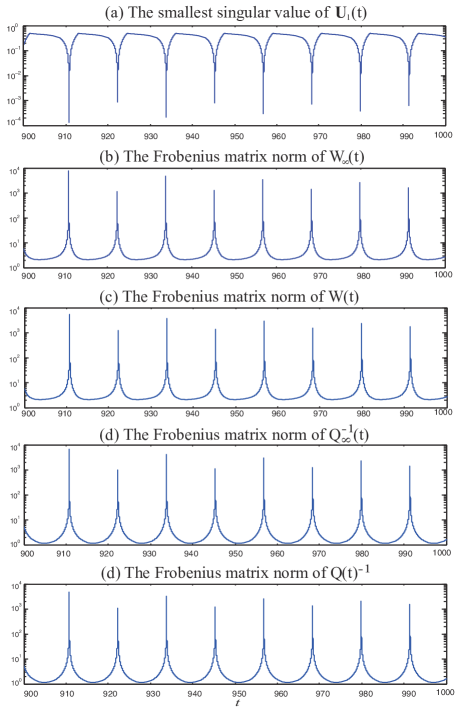
  Figure 1: The smallest singular value of $\mathbf{U}_{1}(t)$, $\|W_{\infty}(t)\|_{F}$, $\|W(t)\|_{F}$, $\|Q_{\infty}^{-1}(t)\|_{F}$ and $\|Q^{-1}(t)\|_{F}$ plotted by the log scale.

  

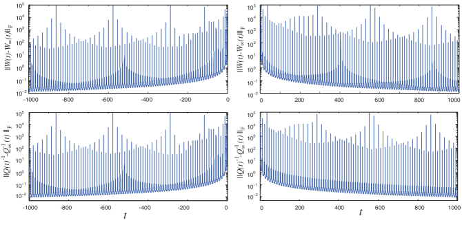
  Figure 2: $\|W(t)-W_{\infty}(t)\|_{F}$ and $\|Q(t)^{-1}-Q_{\infty}^{-1}(t)\|_{F}$ plotted by the log scale for $-1000\leqslant t\leqslant 0$ and for $0\leqslant t\leqslant 1000$.

• Let $\eta:=\gamma=\delta=7.8340$, i.e., we consider the case $x=c$. In this case we have shown in Theorem 4.15 that

  • $W(t)$ converges at the rate $O(t^{-1})$ to a constant matrix $\mathbf{U}_{2,0}\mathbf{U}_{1,0}^{-1}$;

  • $Q(t)^{-1}$ converges at the rate $O(t^{-1})$ to a periodic orbit, $e^{-i\eta t}W_{2}^{-1}e_{n}e_{n}^{H}\mathbf{U}_{1,0}^{-1}$, with period $2\pi/|\eta|$.

  In Figure 3, we show the difference between $W(t)$ and the constant matrix $\mathbf{U}_{2,0}\mathbf{U}_{1,0}^{-1}$ for $-1000\leqslant t\leqslant 0$ and for $0\leqslant t\leqslant 1000$. In Figure 4, we show the Frobenius norm of $Q(t)^{-1}$ and the difference between $Q(t)^{-1}$ and $Q_{\infty}^{-1}(t)=e^{-i\eta t}W_{2}^{-1}e_{n}e_{n}^{H}\mathbf{U}_{1,0}^{-1}$ for $-1000\leqslant t\leqslant 0$ and for $0\leqslant t\leqslant 1000$. We can also see in Figures 3 and 4 that $W(t)$ and $Q(t)^{-1}$ have a blow-up at $t\approx-10$, even though we have shown in Theorem 4.15 that $W(t)$ and $Q(t)^{-1}$ have convergence with the rate $O(t^{-1})$.

  

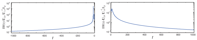
  Figure 3: $\|W(t)-\mathbf{U}_{2,0}\mathbf{U}_{1,0}^{-1}\|_{F}$ for $-1000\leqslant t\leqslant 0$ and for $0\leqslant t\leqslant 1000$.

  

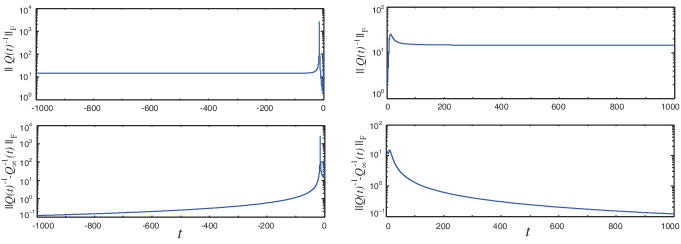
  Figure 4: $\|Q(t)^{-1}\|_{F}$ and $\|Q(t)^{-1}-Q_{\infty}^{-1}(t)\|_{F}$ for $-1000\leqslant t\leqslant 0$ and for $0\leqslant t\leqslant 1000$.

Note that the matrix $\mathfrak{J}$ in Example 4.1 is given, and hence, the solution $W(t)$ can be computed with a good accuracy. For the general $\mathscr{H}$, a number of algorithms have been proposed for solving RDEs (4.3) numerically. These include conventional Runge-Kutta methods and linear multi-step methods [13, 22] if blow-ups are not in the solution. If the solutions have blow-ups, an efficient numerical method developed by [57] can be used for solving the RDEs.

4.3 Asymptotic Analysis of RDE

In this subsection, we will investigate the asymptotic behaviors of $W(t)=P(t)Q(t)^{-1}$ and $Q(t)^{-1}$ as $t\rightarrow\pm\infty$, where $Y(t)=[Q(t)^{\top},P(t)^{\top}]^{\top}$ is the solution of IVP (4.3). Suppose that $\mathcal{S}$ is symplectic such that $\mathcal{S}^{-1}\mathscr{H}\mathcal{S}=\mathfrak{J}$ is of the form in (4.30), where $\mathscr{H}\in\mathbb{C}^{2n\times 2n}$ is the Hamiltonian matrix in (4.3). Since $\mathfrak{J}$ is the combination of the four elementary cases in Subsection 4.2, detailed calculations for the asymptotic analysis are much tedious. However, the procedure is similar to what we have done in Subsection 4.2. Therefore, we only state the asymptotic analysis for the general cases and leave the proofs in Appendix.

Denote $n_{r}$, $n_{e}$, $n_{c}$ and $n_{d}$ be the sizes of $R_{r}$, $R_{e}$, $R_{c}$ and $R_{d}$ in (4.30), respectively. It holds that $n_{r}+n_{e}+n_{c}+n_{d}=n$. Let $n_{cd}=n_{c}+n_{d}$ and $n_{ecd}=n_{e}+n_{c}+n_{d}$. Partitioning $W_{j}$ for $j=1,2$ in (4.35) as

$$\begin{array}[]{cc}W_{j}=\left[\begin{array}[]{cc}W^{j}_{1,1}&W^{j}_{1,2}\\ W^{j}_{2,1}&W^{j}_{2,2}\end{array}\right]&\!\!\!\!\!\!\!\!\begin{array}[]{l}\}n_{r}\\ \}n_{ecd}\end{array}\vspace{-0.3cm}\\ \begin{array}[]{cc}\ \ \ \ \ \ \ \ \underbrace{}_{n_{r}}&\underbrace{}_{n_{ecd}}\end{array}&\end{array}.$$

We first make two assumptions:

Assumption $\mathscr{A}_{+}$.

Assume that $\mathbf{Z}_{1,+}^{-1}=\left[\begin{array}[]{cc}W^{1}_{1,1}&W^{1}_{1,2}\\ W^{2}_{2,1}&W^{2}_{2,2}\end{array}\right]$ is invertible.

Assumption $\mathscr{A}_{-}$.

Assume that $\mathbf{Z}_{1,-}^{-1}=W_{2}$ is invertible.

Remark 4.3.

When we consider four elementary cases mentioned in Subsection 4.2, it follows from Theorem 4.9 that Assumptions $\mathscr{A}_{+}$ and $\mathscr{A}_{-}$ are one of the necessary conditions for the asymptotic analysis as $t\rightarrow\infty$ and $t\rightarrow-\infty$, respectively.

Under the Assumptions $\mathscr{A}_{+}$ and $\mathscr{A}_{-}$, the matrices $\mathbf{Z}_{1,+}$ and $\mathbf{Z}_{1,-}$ exist. We partition $\mathbf{Z}_{1,+}$ and $\mathbf{Z}_{1,-}$ as the block forms

$$\begin{array}[]{c}\mathbf{Z}_{1,+}=\left[\begin{array}[]{cc}\mathbf{Z}^{1}_{r,+}&\mathbf{Z}^{1}_{ecd,+}\end{array}\right]\}n,\vspace{-0.3cm}\\ \begin{array}[]{cc}\ \ \ \ \underbrace{}_{n_{r}}&\ \underbrace{}_{n_{ecd}}\end{array}\end{array}\ \ \begin{array}[]{c}\mathbf{Z}_{1,-}=\left[\begin{array}[]{cc}\mathbf{Z}^{1}_{r,-}&\mathbf{Z}^{1}_{ecd,-}\end{array}\right]\}n.\vspace{-0.3cm}\\ \begin{array}[]{cc}\ \ \ \ \underbrace{}_{n_{r}}&\ \underbrace{}_{n_{ecd}}\end{array}\end{array}$$ (4.256)

From (4.35), we have

$$Y(t)\mathbf{Z}_{1,+}=\mathcal{S}e^{\mathfrak{J}t}\left[\begin{array}[]{c}\mathbf{W}_{1}^{+}\\ \mathbf{W}_{2}^{+}\\ \end{array}\right],\ \ \ \ \ Y(t)\mathbf{Z}_{1,-}=\mathcal{S}e^{\mathfrak{J}t}\left[\begin{array}[]{c}\mathbf{W}_{1}^{-}\\ \mathbf{W}_{2}^{-}\\ \end{array}\right],$$ (4.261)

where $\mathbf{W}_{j}^{+}=W_{j}\mathbf{Z}_{1,+}$ and $\mathbf{W}_{j}^{-}=W_{j}\mathbf{Z}_{1,-}$, for $j=1,2$, are of the forms

$$\mathbf{W}_{1}^{+} =\left[\begin{array}[]{cc}I_{n_{r}}&0\\ \mathbf{W}^{+}_{2,1}&\mathbf{W}^{+}_{ecd}\end{array}\right],\ \ \ \ \mathbf{W}_{2}^{+}=\left[\begin{array}[]{cc}\mathbf{W}^{+}_{1,1}&\mathbf{W}^{+}_{1,2}\\ 0&I_{n_{ecd}}\end{array}\right],$$ (4.262e)

$$\mathbf{W}_{1}^{-} =\left[\begin{array}[]{cc}\mathbf{W}^{-}_{1,1}&\mathbf{W}^{-}_{1,2}\\ \mathbf{W}^{-}_{2,1}&\mathbf{W}^{-}_{ecd}\end{array}\right],\ \ \ \ \mathbf{W}_{2}^{-}=\left[\begin{array}[]{cc}I_{n_{r}}&0\\ 0&I_{n_{ecd}}\end{array}\right].$$ (4.262j)

In order to investigate the asymptotic behavior of $Y(t)$, we partition the symplectic matrix $\mathcal{S}$ in (4.30) and $e^{\mathfrak{J}t}$ in (4.110), respectively, as

$$\mathcal{S}=\left[\begin{array}[]{cc|cc}U_{r}&U_{ecd}&V_{r}&V_{ecd}\end{array}\right]=\left[\begin{array}[]{cc|cc}U^{r}_{1}&U^{ecd}_{1}&V^{r}_{1}&V^{ecd}_{1}\\ \hline\cr U^{r}_{2}&U^{ecd}_{2}&V^{r}_{2}&V^{ecd}_{2}\end{array}\right]$$ (4.266)

and

$$e^{\mathfrak{J}t}=\left[\begin{array}[]{cc|cc}\mathcal{R}_{r}&0&0&0\\ 0&\mathcal{R}_{ecd}&0&\mathcal{D}_{ecd}\\ \hline\cr 0&0&\mathcal{R}_{r}^{-H}&0\\ 0&\mathcal{G}_{ecd}&0&\mathcal{E}_{ecd}\end{array}\right]\equiv\left[\begin{array}[]{cc|cc}\mathcal{R}_{r}(t)&0&0&0\\ 0&\mathcal{R}_{ecd}(t)&0&\mathcal{D}_{ecd}(t)\\ \hline\cr 0&0&\mathcal{R}_{r}(t)^{-H}&0\\ 0&\mathcal{G}_{ecd}(t)&0&\mathcal{E}_{ecd}(t)\end{array}\right],$$ (4.275)

where $\mathcal{R}_{r}=e^{R_{r}t}$ and $R_{r}$ is defined in (4.30).

Let $\mathfrak{r}=\min\{\Re({\rm diag}(R_{r}))\}>0$, where $\Re(z)$ is the real part of $z\in\mathbb{C}$. Then

$$\begin{array}[]{l}\mathcal{R}_{r}^{-1}=o(e^{-\mathfrak{r}t}t^{n_{r}}),\ \ \ \ \text{ as }t\rightarrow\infty,\\ \mathcal{R}_{r}^{H}=o(e^{-\mathfrak{r}|t|}|t|^{n_{r}}),\ \ \text{ as }t\rightarrow-\infty,\end{array}$$ (4.278)

i.e., $\lim_{t\rightarrow\infty}t^{-n_{r}}e^{\mathfrak{r}t}\mathcal{R}_{r}^{-1}=\lim_{t\rightarrow-\infty}|t|^{-n_{r}}e^{\mathfrak{r}|t|}\mathcal{R}_{r}^{H}=0$.

Theorem 4.16.

Assume that $\mathscr{H}$ in (4.3) has Hamiltonian Jordan canonical form $\mathfrak{J}$ in (4.30) and the symplectic matrix $\mathcal{S}$ in (4.30) is of the form in (4.266). Then

• if Assumption $\mathscr{A}_{+}$ holds, then there is a nonsingular matrix

  $$\mathbf{Z}_{2,+}(t)=\mathbf{Z}_{1,+}(\mathcal{R}_{r}^{-1}\oplus I_{n_{ecd}}),$$ (4.279a)

  such that

  $$Y(t)\mathbf{Z}_{2,+}(t)=\left[U_{r},[U_{ecd}|V_{ecd}]\left[\begin{array}[]{c|c}\mathcal{R}_{ecd}&\mathcal{D}_{ecd}\\ \hline\cr\mathcal{G}_{ecd}&\mathcal{E}_{ecd}\end{array}\right]\left[\begin{array}[]{c}\mathbf{W}^{+}_{ecd}\\ \hline\cr I_{n_{ecd}}\end{array}\right]\right]+o(e^{-\mathfrak{r}t}t^{n}),$$ (4.279f)

  as $t\rightarrow\infty$. In particular, if $\mathfrak{J}=\left[\begin{array}[]{c|c}R_{r}&0\\ \hline\cr 0&-R_{r}^{H}\end{array}\right]$, then

  $$\mathbf{Z}_{2,+}(t)=o(e^{-\mathfrak{r}t}t^{n}),\ \ Y(t)\mathbf{Z}_{2,+}(t)=U_{r}+o(e^{-2\mathfrak{r}t}t^{2n}),\ \text{ as }t\rightarrow\infty.$$ (4.280)

• if Assumption $\mathscr{A}_{-}$ holds, then there exists an invertible matrix

  $$\mathbf{Z}_{2,-}(t)=\mathbf{Z}_{1,-}(\mathcal{R}_{r}^{H}\oplus I_{n_{ecd}}),$$ (4.281a)

  such that

  $$Y(t)\mathbf{Z}_{2,-}(t)=\left[V_{r},[U_{ecd}|V_{ecd}]\left[\begin{array}[]{c|c}\mathcal{R}_{ecd}&\mathcal{D}_{ecd}\\ \hline\cr\mathcal{G}_{ecd}&\mathcal{E}_{ecd}\end{array}\right]\left[\begin{array}[]{c}\mathbf{W}^{-}_{ecd}\\ \hline\cr I_{n_{ecd}}\end{array}\right]\right]+o(e^{-\mathfrak{r}|t|}|t|^{n}),$$ (4.281f)

  as $t\rightarrow-\infty$. In particular, if $\mathfrak{J}=\left[\begin{array}[]{c|c}R_{r}&0\\ \hline\cr 0&-R_{r}^{H}\end{array}\right]$, then

  $$\mathbf{Z}_{2,-}(t)=o(e^{-\mathfrak{r}|t|}|t|^{n}),\ \ Y(t)\mathbf{Z}_{2,-}(t)=V_{r}+o(e^{-2\mathfrak{r}|t|}|t|^{2n}),\ \text{ as }t\rightarrow-\infty.$$ (4.282)

Proof.

Suppose that Assumption $\mathscr{A}_{+}$ holds. Since $\mathcal{R}_{r}=e^{R_{r}t}$ is invertible, the matrix $\mathbf{Z}_{2,+}(t)$ defined in (4.279a) is invertible. Plugging (4.262e), (4.266), (4.275) and (4.279a) into (4.261), it follows from (4.278) that

$$Y(t)\mathbf{Z}_{2,+}(t) =\mathcal{S}\left[\begin{array}[]{cc|cc}\mathcal{R}_{r}&0&0&0\\ 0&\mathcal{R}_{ecd}&0&\mathcal{D}_{ecd}\\ \hline\cr 0&0&\mathcal{R}_{r}^{-H}&0\\ 0&\mathcal{G}_{ecd}&0&\mathcal{E}_{ecd}\end{array}\right]\left[\begin{array}[]{cc}\mathcal{R}_{r}^{-1}&0\\ \mathbf{W}^{+}_{2,1}\mathcal{R}_{r}^{-1}&\mathbf{W}^{+}_{ecd}\\ \hline\cr\mathbf{W}^{+}_{1,1}\mathcal{R}_{r}^{-1}&\mathbf{W}^{+}_{1,2}\\ 0&I_{n_{ecd}}\end{array}\right]$$ (4.291)

$$=\mathcal{S}\left[\begin{array}[]{cc}I&0\\ o(e^{-\mathfrak{r}t}t^{n})&\mathcal{R}_{ecd}\mathbf{W}^{+}_{ecd}+\mathcal{D}_{ecd}\\ \hline\cr o(e^{-2\mathfrak{r}t}t^{2n_{r}})&o(e^{-\mathfrak{r}t}t^{n_{r}})\\ o(e^{-\mathfrak{r}t}t^{n_{r}})&\mathcal{G}_{ecd}\mathbf{W}^{+}_{ecd}+\mathcal{E}_{ecd}\end{array}\right]$$ (4.296)

$$=\left[U_{r},[U_{ecd}|V_{ecd}]\left[\begin{array}[]{c|c}\mathcal{R}_{ecd}&\mathcal{D}_{ecd}\\ \hline\cr\mathcal{G}_{ecd}&\mathcal{E}_{ecd}\end{array}\right]\left[\begin{array}[]{c}\mathbf{W}^{+}_{ecd}\\ \hline\cr I_{n_{ecd}}\end{array}\right]\right]+o(e^{-\mathfrak{r}t}t^{n}),$$ (4.301)

as $t\rightarrow\infty$. Hence we obtain (4.279f). In particular, if $\mathfrak{J}=R_{r}\oplus(-R_{r}^{H})$, then (4.280) can be obtained from (4.291) directly.

Suppose that Assumption $\mathscr{A}_{-}$ holds. Since $\mathcal{R}_{r}$ is invertible, the matrix $\mathbf{Z}_{2,-}(t)$ defined in (4.281a) is invertible. Plugging (4.262j), (4.266), (4.275) and (4.281a) into (4.261), it follows from (4.278) that

$$Y(t)\mathbf{Z}_{2,-}(t) =\mathcal{S}\left[\begin{array}[]{cc|cc}\mathcal{R}_{r}&0&0&0\\ 0&\mathcal{R}_{ecd}&0&\mathcal{D}_{ecd}\\ \hline\cr 0&0&\mathcal{R}_{r}^{-H}&0\\ 0&\mathcal{G}_{ecd}&0&\mathcal{E}_{ecd}\end{array}\right]\left[\begin{array}[]{cc}\mathbf{W}^{-}_{1,1}\mathcal{R}_{r}^{H}&\mathbf{W}^{-}_{1,2}\\ \mathbf{W}^{-}_{2,1}\mathcal{R}_{r}^{H}&\mathbf{W}^{-}_{ecd}\\ \hline\cr\mathcal{R}_{r}^{H}&0\\ 0&I_{n_{ecd}}\end{array}\right]$$ (4.310)

$$=\mathcal{S}\left[\begin{array}[]{cc}o(e^{-2\mathfrak{r}|t|}|t|^{2n_{r}})&o(e^{-\mathfrak{r}|t|}|t|^{n_{r}})\\ o(e^{-\mathfrak{r}|t|}|t|^{n})&\mathcal{R}_{ecd}\mathbf{W}^{-}_{ecd}+\mathcal{D}_{ecd}\\ \hline\cr I&0\\ o(e^{-\mathfrak{r}|t|}|t|^{n_{r}})&\mathcal{G}_{ecd}\mathbf{W}^{-}_{ecd}+\mathcal{E}_{ecd}\end{array}\right]$$ (4.315)

$$=\left[V_{r},[U_{ecd}|V_{ecd}]\left[\begin{array}[]{c|c}\mathcal{R}_{ecd}&\mathcal{D}_{ecd}\\ \hline\cr\mathcal{G}_{ecd}&\mathcal{E}_{ecd}\end{array}\right]\left[\begin{array}[]{c}\mathbf{W}^{-}_{ecd}\\ \hline\cr I_{n_{ecd}}\end{array}\right]\right]+o(e^{-\mathfrak{r}|t|}|t|^{n}),$$ (4.320)

as $t\rightarrow-\infty$. Hence we obtain (4.281f). In particular, if $\mathfrak{J}=R_{r}\oplus(-R_{r}^{H})$, then (4.282) can be obtained from (4.310) directly. ∎

By (4.280) and (4.282), we have the following consequence.

Corollary 4.17.

With the same notations of Theorem 4.16, suppose that Assumptions $\mathscr{A}_{+}$ and $\mathscr{A}_{-}$ hold and $\mathfrak{J}=\left[\begin{array}[]{c|c}R_{r}&0\\ \hline\cr 0&-R_{r}^{H}\end{array}\right]$. Let $\mathbf{U}_{j}=U_{j}^{r}$, $\mathbf{V}_{j}=V_{j}^{r}$ for $j=1,2$ and $W(t)=P(t)Q(t)^{-1}$, where $Y(t)=[Q(t)^{\top},P(t)^{\top}]^{\top}$ is the solution of IVP (4.3). If $\mathbf{U}_{1}$ and $\mathbf{V}_{1}$ are invertible, then

$$\begin{array}[]{lll}W(t)=\mathbf{U}_{2}\mathbf{U}_{1}^{-1}+O(e^{-2\mathfrak{r}t}t^{2n}),&Q(t)^{-1}=O(e^{-\mathfrak{r}t}t^{n}),&\text{ as }t\rightarrow\infty,\\ W(t)=\mathbf{V}_{2}\mathbf{V}_{1}^{-1}+O(e^{-2\mathfrak{r}|t|}|t|^{2n}),&Q(t)^{-1}=O(e^{-\mathfrak{r}|t|}|t|^{n}),&\text{ as }t\rightarrow-\infty,\end{array}$$

where $\mathfrak{r}=\min\{\Re({\rm diag}(R_{r}))\}>0$. Here, $\mathbf{U}_{2}\mathbf{U}_{1}^{-1}$ and $\mathbf{V}_{2}\mathbf{V}_{1}^{-1}$ are Hermitian.

Let

$$Y_{ecd,\pm}(t)=[U_{ecd}|V_{ecd}]\left[\begin{array}[]{c|c}\mathcal{R}_{ecd}&\mathcal{D}_{ecd}\\ \hline\cr\mathcal{G}_{ecd}&\mathcal{E}_{ecd}\end{array}\right]\left[\begin{array}[]{c}\mathbf{W}^{\pm}_{ecd}\\ \hline\cr I_{n_{ecd}}\end{array}\right].$$ (4.325)

From (4.279f) and (4.281f), we need to simplify $Y_{ecd,\pm}(t)$ for checking the linear independence of its column space, as $t\rightarrow\pm\infty$. Plugging (4.256) into (4.279a) and (4.281a), it follows from (4.278) that

$$\begin{array}[]{ll}\mathbf{Z}_{2,+}(t)=\left[o(e^{-\mathfrak{r}t}t^{n_{r}}),\mathbf{Z}_{ecd,+}^{1}\right],&\text{ as }t\rightarrow\infty,\\ \mathbf{Z}_{2,-}(t)=\left[o(e^{-\mathfrak{r}|t|}|t|^{n_{r}}),\mathbf{Z}_{ecd,-}^{1}\right],&\text{ as }t\rightarrow-\infty.\end{array}$$ (4.328)

Partition $\mathbf{Z}^{1}_{ecd,\pm}$ in (4.256), $\mathbf{W}_{ecd}^{\pm}$ in (4.262) and $U_{ecd}$, $V_{ecd}$ in (4.266), respectively, as

$$\begin{array}[]{l}\mathbf{Z}^{1}_{ecd,\pm}=\left[\begin{array}[]{cc}\mathbf{Z}^{1}_{e,\pm}&\mathbf{Z}^{1}_{cd,\pm}\end{array}\right]\}n,\vspace{-0.3cm}\\ \begin{array}[]{cc}\hskip 51.21504pt\underbrace{}_{n_{e}}&\ \underbrace{}_{n_{cd}}\end{array}\\ \mathbf{W}_{ecd}^{\pm}=\left[\begin{array}[]{cc}\mathbf{W}_{2,2}^{\pm}&\mathbf{W}_{2,3}^{\pm}\\ \mathbf{W}_{3,2}^{\pm}&\mathbf{W}_{cd}^{\pm}\end{array}\right]\begin{array}[]{l}\}n_{e}\\ \}n_{cd}\end{array}\vspace{-0.3cm}\\ \begin{array}[]{cc}\hskip 51.21504pt\underbrace{}_{n_{e}}&\ \underbrace{}_{n_{cd}}\end{array}\end{array}$$ (4.340)

and

$$U_{ecd}=\left[U_{e},U_{cd}\right]=\left[\begin{array}[]{cc}U^{e}_{1}&U^{cd}_{1}\\ \hline\cr U^{e}_{2}&U^{cd}_{2}\end{array}\right],\ \ V_{ecd}=\left[V_{e},V_{cd}\right]=\left[\begin{array}[]{cc}V^{e}_{1}&V^{cd}_{1}\\ \hline\cr V^{e}_{2}&V^{cd}_{2}\end{array}\right].$$ (4.345)

Let

$$\left[\begin{array}[]{c|c}\mathcal{R}_{cd}&\mathcal{D}_{cd}\\ \hline\cr\mathcal{G}_{cd}&\mathcal{E}_{cd}\end{array}\right]\equiv\left[\begin{array}[]{c|c}\mathcal{R}_{cd}(t)&\mathcal{D}_{cd}(t)\\ \hline\cr\mathcal{G}_{cd}(t)&\mathcal{E}_{cd}(t)\end{array}\right]=\left[\begin{array}[]{c|c}\mathcal{R}_{c}\oplus\mathcal{R}_{d}&\mathcal{D}_{c}\oplus\mathcal{D}_{d}\\ \hline\cr 0\oplus\mathcal{G}_{d}&\mathcal{R}_{c}^{-H}\oplus\mathcal{E}_{d}\end{array}\right],$$ (4.352)

where $\mathcal{R}_{c}$, $\mathcal{R}_{d}$, $\mathcal{D}_{c}$, $\mathcal{D}_{d}$, $\mathcal{G}_{d}$ and $\mathcal{E}_{d}$ are shown in Theorem 4.8. Then

$$\left[\begin{array}[]{c|c}\mathcal{R}_{ecd}&\mathcal{D}_{ecd}\\ \hline\cr\mathcal{G}_{ecd}&\mathcal{E}_{ecd}\end{array}\right]=\left[\begin{array}[]{c|c}\mathcal{R}_{e}\oplus\mathcal{R}_{cd}&\mathcal{D}_{e}\oplus\mathcal{D}_{cd}\\ \hline\cr 0\oplus\mathcal{G}_{cd}&\mathcal{R}_{e}^{-H}\oplus\mathcal{E}_{cd}\end{array}\right],$$

where $\mathcal{R}_{e}\equiv\mathcal{R}_{e}(t)$ and $\mathcal{D}_{e}\equiv\mathcal{D}_{e}(t)$ are shown in (4.110). Denote

$$\mathcal{T}_{e,\pm}\equiv\mathcal{T}_{e,\pm}(t)=\mathcal{R}_{e}\mathbf{W}^{\pm}_{2,2}+\mathcal{D}_{e},$$ (4.353)

where $\mathbf{W}^{\pm}_{2,2}$ is given in (4.340). The proof of the following lemma is left in Appendix.

Lemma 4.18.

Let $\mathcal{R}_{cd}$, $\mathcal{D}_{cd}$, $\mathcal{G}_{cd}$, $\mathcal{E}_{cd}$ and $\mathcal{T}_{e,\pm}$ be of the forms in (4.352) and (4.353), respectively. Let

$$\mathcal{I}_{\pm}=\{t\in\mathbb{R}|\mathcal{T}_{e,\pm}\text{ and }\mathcal{R}_{cd}(\mathbf{W}^{\pm}_{cd}-\mathbf{W}^{\pm}_{3,2}\mathcal{T}_{e,\pm}^{-1}\mathcal{R}_{e}\mathbf{W}^{\pm}_{2,3})+\mathcal{D}_{cd}\text{ are invertible}\},$$ (4.354)

where $\mathbf{W}^{\pm}_{cd}$, $\mathbf{W}^{\pm}_{3,2}$ and $\mathbf{W}^{\pm}_{2,3}$ are given in (4.340). Then there are nonsingular matrices, $Z_{ecd,+}(t)$ for $t\in\mathcal{I}_{+}$ and $Z_{ecd,-}(t)$ for $t\in\mathcal{I}_{-}$, of the forms

$$\begin{array}[]{l}Z_{ecd,\pm}(t)=\left[\begin{array}[]{cc}O(t^{-1})&O(t^{-1})\\ O(t^{-1})&I_{n_{cd}}\end{array}\right],\ \ \ \text{ as }t\rightarrow\pm\infty,\vspace{-0.3cm}\\ \begin{array}[]{cc}\hskip 68.28644pt\underbrace{}_{n_{e}}&\ \ \ \ \underbrace{}_{n_{cd}}\end{array}\end{array}$$ (4.355f)

such that

$$Y_{ecd,\pm}(t)Z_{ecd,\pm}(t)=\left[U_{e},[U_{cd}|V_{cd}]\left[\begin{array}[]{c|c}\mathcal{R}_{cd}&\mathcal{D}_{cd}\\ \hline\cr\mathcal{G}_{cd}&\mathcal{E}_{cd}\end{array}\right]\left[\begin{array}[]{c}\mathbf{W}^{\pm}_{cd}+O(t^{-1})\\ \hline\cr I\end{array}\right]\right]+O(t^{-1}),$$ (4.355k)

as $t\rightarrow\pm\infty$, respectively, where $U_{e}$, $U_{cd}$ and $V_{cd}$ are given in (4.345) and $Y_{ecd,\pm}(t)$ and $\mathbf{W}^{\pm}_{cd}$ are given in (4.325) and (4.340), respectively.

Denote

$$\mathbf{Z}_{3,\pm}(t)=\mathbf{Z}_{2,\pm}(t)(I_{n_{r}}\oplus Z_{ecd,\pm}(t)),\text{ for }t\in\mathcal{I}_{\pm}.$$

From Theorem 4.16, Lemma 4.18 and (4.328), we then have the theorem.

Theorem 4.19.

With the same notations of Theorem 4.16, where $U_{ecd}$ and $V_{ecd}$ are of the forms in (4.345). Let $\mathfrak{r}=\min\{\Re({\rm diag}(R_{r}))\}>0$. Then

• if Assumption $\mathscr{A}_{+}$ holds, then there is a nonsingular matrix $\mathbf{Z}_{3,+}(t)$ with

  $$\begin{array}[]{l}\mathbf{Z}_{3,+}(t)=\left[\begin{array}[]{ccc}o(e^{-\mathfrak{r}t}t^{n_{r}})&O(t^{-1})&\mathbf{Z}^{1}_{cd,+}+O(t^{-1})\end{array}\right]\vspace{-0.3cm}\\ \begin{array}[]{ccc}\hskip 56.9055pt\underbrace{\ \ \ \ \ \ \ \ \ }_{n_{r}}&\ \ \ \ \underbrace{}_{n_{e}}&\ \ \underbrace{\ \ \ \ \ \ \ \ \ \ \ \ \ \ \ }_{n_{cd}}\end{array}\end{array}$$ (4.356e)

  for $$t\in\mathcal{I}_{+}$$ such that

  $$Y(t)\mathbf{Z}_{3,+}(t)=\left[U_{r}+o(e^{-\mathfrak{r}t}t^{n}),\left[U_{e},[U_{cd}|V_{cd}]\left[\begin{array}[]{c|c}\mathcal{R}_{cd}&\mathcal{D}_{cd}\\ \hline\cr\mathcal{G}_{cd}&\mathcal{E}_{cd}\end{array}\right]\left[\begin{array}[]{c}\mathbf{W}^{+}_{cd}+O(t^{-1})\\ \hline\cr I\end{array}\right]\right]+O(t^{-1})\right],$$ (4.356j)

  as $t\rightarrow\infty$, where $\mathbf{Z}^{1}_{cd,+}$ and $\mathbf{W}^{+}_{cd}$ are given in (4.340);

• if Assumption $\mathscr{A}_{-}$ holds, then there is a nonsingular matrix $\mathbf{Z}_{3,-}(t)$ with

  $$\begin{array}[]{l}\mathbf{Z}_{3,-}(t)=\left[\begin{array}[]{ccc}o(e^{-\mathfrak{r}|t|}|t|^{n_{r}})&O(t^{-1})&\mathbf{Z}^{1}_{cd,-}+O(t^{-1})\end{array}\right]\vspace{-0.3cm}\\ \begin{array}[]{ccc}\hskip 56.9055pt\underbrace{\ \ \ \ \ \ \ \ \ \ \ }_{n_{r}}&\ \ \ \ \underbrace{}_{n_{e}}&\ \ \ \underbrace{\ \ \ \ \ \ \ \ \ \ \ \ \ \ \ }_{n_{cd}}\end{array}\end{array}$$ (4.357e)

  for $$t\in\mathcal{I}_{-}$$ such that

  $$Y(t)\mathbf{Z}_{3,-}(t)=\left[V_{r}+o(e^{-\mathfrak{r}|t|}|t|^{n}),\left[U_{e},[U_{cd}|V_{cd}]\left[\begin{array}[]{c|c}\mathcal{R}_{cd}&\mathcal{D}_{cd}\\ \hline\cr\mathcal{G}_{cd}&\mathcal{E}_{cd}\end{array}\right]\left[\begin{array}[]{c}\mathbf{W}^{-}_{cd}+O(t^{-1})\\ \hline\cr I\end{array}\right]\right]+O(t^{-1})\right],$$ (4.357j)

  as $t\rightarrow-\infty$, where $\mathbf{Z}^{1}_{cd,-}$ and $\mathbf{W}^{-}_{cd}$ are given in (4.340).

In the case that $\mathcal{R}_{cd}$, $\mathcal{D}_{cd}$, $\mathcal{G}_{cd}$ and $\mathcal{E}_{cd}$ are absent, we have an immediate consequence.

Corollary 4.20.

With the same notations of Theorem 4.19, suppose that Assumptions $\mathscr{A}_{+}$ and $\mathscr{A}_{-}$ hold and

$$\mathfrak{J}=\mathfrak{J}_{re}\equiv\left[\begin{array}[]{cc|cc}R_{r}&0&0&0\\ 0&R_{e}&0&D_{e}\\ \hline\cr 0&0&-R_{r}^{H}&0\\ 0&0&0&-R_{e}^{H}\end{array}\right].$$ (4.362)

Let $\mathbf{U}_{j,+}=[U_{j}^{r},U_{j}^{e}]$, $\mathbf{U}_{j,-}=[V_{j}^{r},U_{j}^{e}]$ for $j=1,2$ and $W(t)=P(t)Q(t)^{-1}$, where $Y(t)=[Q(t)^{\top},P(t)^{\top}]^{\top}$ is the solution of IVP (4.3). If $\mathbf{U}_{1,+}$ and $\mathbf{U}_{1,-}$ are invertible, then

$$\begin{array}[]{lll}W(t)=\mathbf{U}_{2,+}\mathbf{U}^{-1}_{1,+}+O(t^{-1}),&Q(t)^{-1}=O(t^{-1}),&\text{ as }t\rightarrow\infty,\\ W(t)=\mathbf{U}_{2,-}\mathbf{U}^{-1}_{1,-}+O(t^{-1}),&Q(t)^{-1}=O(t^{-1}),&\text{ as }t\rightarrow-\infty.\end{array}$$

Here, $\mathbf{U}_{2,\pm}\mathbf{U}^{-1}_{1,\pm}$ is Hermitian.

Suppose that those submatrices $R_{d}$, $D_{d}$ and $G_{d}$ of $\mathfrak{J}$ in (4.30) are absent and that $\mathfrak{J}_{c}=\left[\begin{array}[]{cc}R_{c}&D_{c}\\ 0&-R_{c}^{H}\end{array}\right]$ is of the elementary case with the form in (4.113), where $R_{c}$ and $D_{c}$ are submatrices of $\mathfrak{J}$. Then $U_{cd}=U_{c}$ and $V_{cd}=V_{c}$. Partition

$$U_{c}\equiv\left[\begin{array}[]{c}U^{c}_{1}\\ \hline\cr U^{c}_{2}\end{array}\right]=\left[\begin{array}[]{cc}U^{c}_{1,1}&u^{c}_{1,2}\\ \hline\cr U^{c}_{2,1}&u^{c}_{2,2}\end{array}\right],\ \ V_{c}\equiv\left[\begin{array}[]{c}V^{c}_{1}\\ \hline\cr V^{c}_{2}\end{array}\right]=\left[\begin{array}[]{cc}V^{c}_{1,1}&v^{c}_{1,2}\\ \hline\cr V^{c}_{2,1}&v^{c}_{2,2}\end{array}\right].$$ (4.371)

We state the corollary but omit its proof, as it is an easy combination of Theorems 4.15 and 4.19.

Corollary 4.21.

With the same notations of Theorem 4.19, suppose that Assumptions $\mathscr{A}_{+}$ and $\mathscr{A}_{-}$ hold, and

$$\mathfrak{J}=\left[\begin{array}[]{ccc|ccc}R_{r}&0&0&0&0&0\\ 0&R_{e}&0&0&D_{e}&0\\ 0&0&R_{c}&0&0&D_{c}\\ \hline\cr 0&0&0&-R_{r}^{H}&0&0\\ 0&0&0&0&-R_{e}^{H}&0\\ 0&0&0&0&0&-R_{c}^{H}\end{array}\right],$$ (4.372g)

where

$$\left[\begin{array}[]{cc}R_{c}&D_{c}\\ 0&-R_{c}^{H}\end{array}\right]\text{ is of the elementary case with }\sigma(R_{c})=\{i\eta\}.$$ (4.372j)

Let $f_{u}^{\pm}$, $g_{u}^{\pm}$, $f_{v}^{\pm}$ and $g_{v}^{\pm}$ be the constants defined in (4.149e) with $\mathbf{W}$ being replaced by $\mathbf{W}_{cd}^{\pm}$, where $\mathbf{W}_{cd}^{\pm}$ is given in (4.340). Denote

$$\begin{array}[]{l}\mathbf{U}_{1,0}^{c,\pm}=[U_{1,1}^{c},(f_{u}^{\pm}+g_{u}^{\pm})u_{1,2}^{c}+(f_{v}^{\pm}+g_{v}^{\pm})v_{1,2}^{c}],\\ \mathbf{U}_{2,0}^{c,\pm}=[U_{2,1}^{c},(f_{u}^{\pm}+g_{u}^{\pm})u_{2,2}^{c}+(f_{v}^{\pm}+g_{v}^{\pm})v_{2,2}^{c}],\end{array}$$

where $U_{1,1}^{c}$, $U_{2,1}^{c}$, $u_{1,2}^{c}$, $u_{2,2}^{c}$, $v_{1,2}^{c}$ and $v_{2,2}^{c}$ are defined in (4.371). Let

$$\mathbf{U}_{j,+}=[U_{j}^{r},U_{j}^{e},\mathbf{U}_{j,0}^{c,+}],\ \ \mathbf{U}_{j,-}=[V_{j}^{r},U_{j}^{e},\mathbf{U}_{j,0}^{c,-}],$$ (4.373)

for $j=1,2$. If $\mathbf{U}_{1,+}$ and $\mathbf{U}_{1,-}$ are invertible, then

$$\begin{array}[]{lll}W(t)=\mathbf{U}_{2,+}\mathbf{U}^{-1}_{1,+}+O(t^{-1}),&Q(t)^{-1}=e^{-i\eta t}\mathbf{Z}_{cd,+}^{1}e_{n_{cd}}e_{n}^{H}\mathbf{U}^{-1}_{1,+}+O(t^{-1}),&\text{ as }t\rightarrow\infty,\\ W(t)=\mathbf{U}_{2,-}\mathbf{U}^{-1}_{1,-}+O(t^{-1}),&Q(t)^{-1}=e^{-i\eta t}\mathbf{Z}_{cd,-}^{1}e_{n_{cd}}e_{n}^{H}\mathbf{U}^{-1}_{1,-}+O(t^{-1}),&\text{ as }t\rightarrow-\infty,\end{array}$$

where $\mathbf{Z}_{cd,\pm}^{1}$ is defined in (4.340). Here $\mathbf{U}_{2,\pm}\mathbf{U}^{-1}_{1,\pm}$ is Hermitian.

From (4.356j) and (4.357j), we need to simplify the linear independence of the column space of

$$Y_{cd,\pm}(t)=\left[U_{cd}|V_{cd}\right]\left[\begin{array}[]{c|c}\mathcal{R}_{cd}&\mathcal{D}_{cd}\\ \hline\cr\mathcal{G}_{cd}&\mathcal{E}_{cd}\end{array}\right]\left[\begin{array}[]{c}\mathbf{W}^{\pm}_{cd}+O(t^{-1})\\ \hline\cr I\end{array}\right],$$ (4.378)

as $t\rightarrow\pm\infty$, respectively. Let

$$\begin{array}[]{ll}\mathcal{R}_{cd}\equiv\mathcal{R}_{cd}(t)={\rm diag}(\mathbf{B}_{1},\ldots,\mathbf{B}_{\mu}),&\mathcal{D}_{cd}\equiv\mathcal{D}_{cd}(t)={\rm diag}(\mathbf{D}_{1},\ldots,\mathbf{D}_{\mu}),\\ \mathcal{G}_{cd}\equiv\mathcal{G}_{cd}(t)={\rm diag}(\mathbf{G}_{1},\ldots,\mathbf{G}_{\mu}),&\mathcal{E}_{cd}\equiv\mathcal{E}_{cd}(t)={\rm diag}(\mathbf{E}_{1},\ldots,\mathbf{E}_{\mu}),\end{array}$$ (4.381)

where $\mu=\mu_{c}+\mu_{d}$,

$$\begin{array}[]{ll}\mathbf{B}_{\ell}\equiv\mathbf{B}_{\ell}(t)=\left[\begin{array}[]{cc}\Phi_{m_{\ell},n_{\ell}}&\phi_{m_{\ell},n_{\ell}}^{1}\\ 0&\omega_{11}^{\ell}\end{array}\right],&\mathbf{D}_{\ell}\equiv\mathbf{D}_{\ell}(t)=\left[\begin{array}[]{cc}\widehat{\Gamma}_{m_{\ell}+1,n_{\ell}+1}^{2m_{\ell},2n_{\ell}}&\phi_{m_{\ell},n_{\ell}}^{2}\\ \widehat{\psi}_{m_{\ell},n_{\ell}}^{1^{H}}&\omega_{12}^{\ell}\end{array}\right],\\ \mathbf{G}_{\ell}\equiv\mathbf{G}_{\ell}(t)=\left[\begin{array}[]{cc}0&0\\ 0&\omega_{21}^{\ell}\end{array}\right],&\mathbf{E}_{\ell}\equiv\mathbf{E}_{\ell}(t)=\left[\begin{array}[]{cc}\widehat{\Phi}_{m_{\ell},n_{\ell}}&0\\ \widehat{\psi}_{m_{\ell},n_{\ell}}^{2^{H}}&\omega_{22}^{\ell}\end{array}\right],\end{array}$$ (4.392)

and $\Phi_{m_{\ell},n_{\ell}}$, $\widehat{\Gamma}_{m_{\ell}+1,n_{\ell}+1}^{2m_{\ell},2n_{\ell}}$, $\phi_{m_{\ell},n_{\ell}}^{1}$, $\phi_{m_{\ell},n_{\ell}}^{2}$, $\widehat{\psi}_{m_{\ell},n_{\ell}}^{1^{H}}$, $\widehat{\psi}_{m_{\ell},n_{\ell}}^{2^{H}}$, $\omega^{\ell}_{11}$, $\omega_{12}^{\ell}$, $\omega_{21}^{\ell}$ and $\omega_{22}^{\ell}$ are defined in (4.101) in which $\gamma$ and $\eta$ are replaced by $\gamma_{\ell}$ and $\delta_{\ell}$, respectively, and $\beta$ is replaced by $\beta^{cd}_{\ell}\in\{-1,1\}$ for $\ell=1,\ldots,\mu$. Note that $\gamma_{\ell}=\delta_{\ell}$, $\beta^{cd}_{\ell}=\beta^{c}_{\ell}$ when $\ell\leqslant\mu_{c}$ and $\gamma_{\ell}\neq\delta_{\ell}$, $\beta^{cd}_{\ell}=\beta^{d}_{\ell}$ when $\mu_{c}<\ell\leqslant\mu$ . Let $\varkappa_{\ell}=m_{\ell}+n_{\ell}+1$. Denote

$$\begin{array}[]{l}\hat{\omega}^{\ell}_{11}\equiv\hat{\omega}^{\ell}_{11}(t)=\frac{1}{2}[(-1)^{m_{\ell}}e^{i\gamma_{\ell}t}+(-1)^{n_{\ell}}e^{i\delta_{\ell}t}],\\ \hat{\omega}^{\ell}_{12}\equiv\hat{\omega}^{\ell}_{12}(t)=\frac{1}{2}[-i\beta^{cd}_{\ell}((-1)^{m_{\ell}}e^{i\gamma_{\ell}t}-(-1)^{n_{\ell}}e^{i\delta_{\ell}t})],\\ \hat{\omega}^{\ell}_{21}\equiv\hat{\omega}^{\ell}_{21}(t)=\frac{1}{2}[i\beta^{cd}_{\ell}((-1)^{m_{\ell}}e^{i\gamma_{\ell}t}-(-1)^{n_{\ell}}e^{i\delta_{\ell}t})],\\ \hat{\omega}^{\ell}_{22}\equiv\hat{\omega}^{\ell}_{22}(t)=\frac{1}{2}[(-1)^{m_{\ell}}e^{i\gamma_{\ell}t}+(-1)^{n_{\ell}}e^{i\delta_{\ell}t}],\\ \end{array}$$ (4.397)

where $\ell\in\{1,2,\ldots,\mu\}$.

In the following lemma, we consider the special case with $\mu=2$, i.e., $\mathcal{R}_{cd}$, $\mathcal{D}_{cd}$, $\mathcal{G}_{cd}$ and $\mathcal{E}_{cd}$ in (4.381) have 2 diagonal blocks. The proof is left in Appendix. For the general case, a similar result can be obtained by using the same procedure of proof.

Lemma 4.22.

Suppose that

$$\mathcal{R}_{cd}=\mathbf{B}_{1}\oplus\mathbf{B}_{2},\ \ \mathcal{D}_{cd}=\mathbf{D}_{1}\oplus\mathbf{D}_{2},\ \ \mathcal{G}_{cd}=\mathbf{G}_{1}\oplus\mathbf{G}_{2},\ \ \mathcal{E}_{cd}=\mathbf{E}_{1}\oplus\mathbf{E}_{2},$$ (4.398)

where $\mathbf{B}_{j},\mathbf{D}_{j},\mathbf{G}_{j},\mathbf{E}_{j}\in\mathbb{C}^{\varkappa_{j}\times\varkappa_{j}}$ are defined in (4.392). Let

$$\begin{array}[]{cr}\mathbf{W}=\left[\begin{array}[]{c|c}\mathbf{W}_{11}&\mathbf{W}_{12}\\ \hline\cr\mathbf{W}_{21}&\mathbf{W}_{22}\end{array}\right]&\!\!\!\!\!\!\!\!\begin{array}[]{c}\}\varkappa_{1}\\ \}\varkappa_{2}\end{array}\vspace{-0.3cm}\\ \ \ \ \ \ \ \ \underbrace{}_{\varkappa_{1}}\ \ \underbrace{}_{\varkappa_{2}}&\end{array}$$ (4.405)

be a constant matrix. Then there is a nonsingular matrix $\Omega(t)$ with

$$\Omega(t)=\left[\begin{array}[]{c|c}e_{\varkappa_{1}}e_{\varkappa_{1}}^{H}&0\\ \hline\cr 0&e_{\varkappa_{2}}e_{\varkappa_{2}}^{H}\end{array}\right]+O(t^{-1})$$

such that

$$\left[\begin{array}[]{c|c}\mathcal{R}_{cd}&\mathcal{D}_{cd}\\ \hline\cr\mathcal{G}_{cd}&\mathcal{E}_{cd}\end{array}\right]\left[\begin{array}[]{c}\mathbf{W}\\ \hline\cr I\end{array}\right]\Omega(t)=\left[\begin{array}[]{cc|cc}I&0&0&0\\ 0&\hat{\omega}^{1}_{11}\mathbf{w}_{11}+\hat{\omega}^{1}_{12}&0&\hat{\omega}^{1}_{11}\mathbf{w}_{12}\\ 0&0&I&0\\ 0&\hat{\omega}^{2}_{11}\mathbf{w}_{21}&0&\hat{\omega}^{2}_{11}\mathbf{w}_{22}+\hat{\omega}^{2}_{12}\\ \hline\cr 0&0&0&0\\ 0&\hat{\omega}^{1}_{21}\mathbf{w}_{11}+\hat{\omega}^{1}_{22}&0&\hat{\omega}^{1}_{21}\mathbf{w}_{12}\\ 0&0&0&0\\ 0&\hat{\omega}^{2}_{21}\mathbf{w}_{21}&0&\hat{\omega}^{2}_{21}\mathbf{w}_{22}+\hat{\omega}^{2}_{22}\end{array}\right]+O(t^{-1}),$$ (4.418)

as $t\rightarrow\pm\infty$, where $\mathbf{w}_{jk}=\mathbf{W}_{jk}(\varkappa_{j},\varkappa_{k})\in\mathbb{C}$ and $\hat{\omega}^{\ell}_{jk}$ are given in (4.397) for $\ell,j,k=1,2$.

Partition $\mathbf{W}_{cd}^{\pm}$, $\mathbf{Z}_{cd,\pm}^{1}$ in (4.340), $U_{cd}$, $V_{cd}$ in (4.345) and identity matrix $I_{n_{cd}}$, respectively, as

$$\begin{array}[]{cr}\mathbf{W}_{cd}^{\pm}=\left[\begin{array}[]{cccc}\mathbf{W}_{cd,11}^{\pm}&\mathbf{W}_{cd,12}^{\pm}&\cdots&\mathbf{W}_{cd,1\mu}^{\pm}\\ \mathbf{W}_{cd,21}^{\pm}&\mathbf{W}_{cd,22}^{\pm}&\cdots&\mathbf{W}_{cd,2\mu}^{\pm}\\ \vdots&\vdots&&\vdots\\ \mathbf{W}_{cd,\mu 1}^{\pm}&\mathbf{W}_{cd,\mu 2}^{\pm}&\cdots&\mathbf{W}_{cd,\mu\mu}^{\pm}\end{array}\right]&\!\!\!\!\!\!\!\!\begin{array}[]{c}\}\varkappa_{1}\\ \}\varkappa_{2}\\ \vdots\\ \}\varkappa_{\mu}\end{array}\vspace{-0.3cm}\\ \ \ \ \ \ \ \ \ \ \ \underbrace{\ \ \ \ \ \ \ }_{\varkappa_{1}}\ \ \ \ \underbrace{\ \ \ \ \ \ \ }_{\varkappa_{2}}\ \hskip 36.98866pt\underbrace{\ \ \ \ \ \ \ }_{\varkappa_{\mu}}&\end{array}$$

$$\begin{array}[]{l}\mathbf{Z}_{cd,\pm}^{1}=\left[\begin{array}[]{cc|cc|c|cc}\mathbf{Z}_{cd,1}^{\pm}&\mathbf{z}_{cd,1}^{\pm}&\mathbf{Z}_{cd,2}^{\pm}&\mathbf{z}_{cd,2}^{\pm}&\cdots&\mathbf{Z}_{cd,\mu}^{\pm}&\mathbf{z}_{cd,\mu}^{\pm}\end{array}\right]\}n,\vspace{-0.2cm}\\ \hskip 51.21504pt\underbrace{}_{\varkappa_{1}-1}\ \ \underbrace{}_{1}\ \ \ \underbrace{}_{\varkappa_{2}-1}\ \ \underbrace{}_{1}\ \hskip 31.2982pt\underbrace{}_{\varkappa_{\mu}-1}\ \ \underbrace{}_{1}\\ U_{cd}\equiv\left[\begin{array}[]{c}U^{cd}_{1}\\ \hline\cr U^{cd}_{2}\end{array}\right]=\left[\begin{array}[]{cc|cc|c|cc}U^{cd}_{1,1}&u^{cd}_{1,1}&U^{cd}_{2,1}&u^{cd}_{2,1}&\cdots&U^{cd}_{\mu,1}&u^{cd}_{\mu,1}\\ \hline\cr U^{cd}_{1,2}&u^{cd}_{1,2}&U^{cd}_{2,2}&u^{cd}_{2,2}&\cdots&U^{cd}_{\mu,2}&u^{cd}_{\mu,2}\end{array}\right],\vspace{-0.2cm}\\ \hskip 99.58464pt\underbrace{}_{\varkappa_{1}-1}\ \underbrace{}_{1}\ \ \underbrace{}_{\varkappa_{2}-1}\ \underbrace{}_{1}\ \hskip 31.2982pt\underbrace{}_{\varkappa_{\mu}-1}\ \underbrace{}_{1}\\ V_{cd}\equiv\left[\begin{array}[]{c}V^{cd}_{1}\\ \hline\cr V^{cd}_{2}\end{array}\right]=\left[\begin{array}[]{cc|cc|c|cc}V^{cd}_{1,1}&v^{cd}_{1,1}&V^{cd}_{2,1}&v^{cd}_{2,1}&\cdots&V^{cd}_{\mu,1}&v^{cd}_{\mu,1}\\ \hline\cr V^{cd}_{1,2}&v^{cd}_{1,2}&V^{cd}_{2,2}&v^{cd}_{2,2}&\cdots&V^{cd}_{\mu,2}&v^{cd}_{\mu,2}\end{array}\right],\vspace{-0.2cm}\\ \hskip 99.58464pt\underbrace{}_{\varkappa_{1}-1}\ \underbrace{}_{1}\ \underbrace{}_{\varkappa_{2}-1}\ \underbrace{}_{1}\ \hskip 25.6073pt\underbrace{}_{\varkappa_{\mu}-1}\ \underbrace{}_{1}\\ I_{n_{cd}}=\left[\begin{array}[]{cc|cc|c|cc}\mathbf{I}^{cd}_{1}&e_{\varkappa_{1}}&\mathbf{I}^{cd}_{2}&e_{\varkappa_{1}+\varkappa_{2}}&\cdots&\mathbf{I}^{cd}_{\mu}&e_{n_{cd}}\end{array}\right]\}n_{cd}.\vspace{-0.2cm}\\ \hskip 36.98866pt\underbrace{}_{\varkappa_{1}-1}\ \underbrace{}_{1}\ \underbrace{}_{\varkappa_{2}-1}\ \ \underbrace{}_{1}\ \hskip 31.2982pt\underbrace{}_{\varkappa_{\mu}-1}\ \underbrace{}_{1}\end{array}$$

Then we denote some constant matrices

$$\begin{array}[]{l}\widehat{U}_{cd}\equiv\left[\begin{array}[]{c}\widehat{U}^{cd}_{1}\\ \hline\cr\widehat{U}^{cd}_{2}\end{array}\right]=\left[\begin{array}[]{c|c|c|c}U^{cd}_{1,1}&U^{cd}_{2,1}&\cdots&U^{cd}_{\mu,1}\\ \hline\cr U^{cd}_{1,2}&U^{cd}_{2,2}&\cdots&U^{cd}_{\mu,2}\end{array}\right],\\ \mathfrak{U}_{cd}\equiv\left[\begin{array}[]{c|c}\mathfrak{U}^{cd}_{u,1}&\mathfrak{U}^{cd}_{v,1}\\ \hline\cr\mathfrak{U}^{cd}_{u,2}&\mathfrak{U}^{cd}_{v,2}\end{array}\right]=\left[\begin{array}[]{cccc|cccc}u^{cd}_{1,1}&u^{cd}_{2,1}&\cdots&u^{cd}_{\mu,1}&v^{cd}_{1,1}&v^{cd}_{2,1}&\cdots&v^{cd}_{\mu,1}\\ \hline\cr u^{cd}_{1,2}&u^{cd}_{2,2}&\cdots&u^{cd}_{\mu,2}&v^{cd}_{1,2}&v^{cd}_{2,2}&\cdots&v^{cd}_{\mu,2}\end{array}\right],\\ \mathfrak{U}^{cd}_{u}=\left[\begin{array}[]{c}\mathfrak{U}^{cd}_{u,1}\\ \mathfrak{U}^{cd}_{u,2}\end{array}\right],\ \ \ \ \mathfrak{U}^{cd}_{v}=\left[\begin{array}[]{c}\mathfrak{U}^{cd}_{v,1}\\ \mathfrak{U}^{cd}_{v,2}\end{array}\right],\\ \mathsf{E}_{\mu}\equiv\left[\begin{array}[]{c}0\\ I_{\mu}\end{array}\right]\in\mathbb{C}^{n\times\mu},\\ \mathfrak{Z}_{cd}^{\pm}\equiv\left[\begin{array}[]{cccc}\mathbf{z}_{cd,1}^{\pm}&\mathbf{z}_{cd,2}^{\pm}&\cdots&\mathbf{z}_{cd,\mu}^{\pm}\end{array}\right]\in\mathbb{C}^{n\times\mu},\\ \mathfrak{W}_{cd}^{\pm}\equiv\left[\begin{array}[]{cccc}\mathbf{w}_{cd,11}^{\pm}&\mathbf{w}_{cd,12}^{\pm}&\cdots&\mathbf{w}_{cd,1\mu}^{\pm}\\ \mathbf{w}_{cd,21}^{\pm}&\mathbf{w}_{cd,22}^{\pm}&\cdots&\mathbf{w}_{cd,2\mu}^{\pm}\\ \vdots&&\ddots&\vdots\\ \mathbf{w}_{cd,\mu 1}^{\pm}&\mathbf{w}_{cd,\mu 2}^{\pm}&\cdots&\mathbf{w}_{cd,\mu\mu}^{\pm}\end{array}\right],\\ P_{cd}\equiv\left[\begin{array}[]{c|c|c|c|cccc}\mathbf{I}^{cd}_{1}&\mathbf{I}^{cd}_{2}&\cdots&\mathbf{I}^{cd}_{\mu}&e_{\varkappa_{1}}&e_{\varkappa_{1}+\varkappa_{2}}&\cdots&e_{n_{cd}}\end{array}\right]\in\mathbb{C}^{n_{cd}\times n_{cd}},\end{array}$$ (4.446)

where $\mathbf{w}_{cd,j\ell}^{\pm}=\mathbf{W}_{cd,j\ell}^{\pm}(\varkappa_{j},\varkappa_{\ell})$ for $j,\ell\in\{1,2,\ldots,\mu\}$.

Note that equations (4.356j) and (4.357j) have the over-estimate form

$$Y(t)\mathbf{Z}_{3,\pm}(t)=\left[\mathbf{U}_{re,\pm},Y_{cd,\pm}(t)\right]+O(t^{-1}),$$

as $t\rightarrow\pm\infty$, where $Y_{cd,\pm}(t)$ is defined in (4.378) and

$$\mathbf{U}_{re,+}\equiv\left[\begin{array}[]{c}\mathbf{U}^{re,+}_{1}\\ \hline\cr\mathbf{U}^{re,+}_{2}\end{array}\right]=\left[\begin{array}[]{cc}U^{r}_{1}&U^{e}_{1}\\ \hline\cr U^{r}_{2}&U^{e}_{2}\end{array}\right],\ \ \ \mathbf{U}_{re,-}\equiv\left[\begin{array}[]{c}\mathbf{U}^{re,-}_{1}\\ \hline\cr\mathbf{U}^{re,-}_{2}\end{array}\right]=\left[\begin{array}[]{cc}V^{r}_{1}&U^{e}_{1}\\ \hline\cr V^{r}_{2}&U^{e}_{2}\end{array}\right].$$ (4.455)

By applying the same procedure of proof of Lemma 4.22 to $Y_{cd,\pm}(t)$, there is a nonsingular matrix $\Omega_{\pm}(t)=I_{n_{r}+n_{e}}\oplus\left({\rm diag}(e_{\varkappa_{1}}e_{\varkappa_{1}}^{H},\cdots,e_{\varkappa_{\mu}}e_{\varkappa_{\mu}}^{H})+O(t^{-1})\right)$ as $t\rightarrow\pm\infty$ and a permutation matrix $\mathbf{P}_{cd}=I_{n_{r}+n_{e}}\oplus P_{cd}$, where $P_{cd}$ is given in (4.446) such that

$$Y(t)\mathbf{Z}_{3,\pm}(t)\Omega_{\pm}(t)\mathbf{P}_{cd}=\left[\mathbf{U}_{re,\pm},\widehat{U}_{cd},\mathfrak{U}_{cd}\Delta_{\pm}(t)\right]+O(t^{-1}),$$

where $\mathbf{U}_{re,\pm}$ is defined in (4.455), $\widehat{U}_{cd}$, $\mathfrak{U}_{cd}$ and $\mathfrak{W}_{cd}^{\pm}$ are given in (4.446),

$$\Delta_{\pm}(t)\equiv\left[\begin{array}[]{c}\Delta_{u}^{\pm}(t)\\ \Delta_{v}^{\pm}(t)\end{array}\right]=\left[\begin{array}[]{l}{\rm diag}(\hat{\omega}_{11}^{1},\hat{\omega}_{11}^{2},\cdots,\hat{\omega}_{11}^{\mu})\mathfrak{W}_{cd}^{\pm}+{\rm diag}(\hat{\omega}_{12}^{1},\hat{\omega}_{12}^{2},\cdots,\hat{\omega}_{12}^{\mu})\\ {\rm diag}(\hat{\omega}_{21}^{1},\hat{\omega}_{21}^{2},\cdots,\hat{\omega}_{21}^{\mu})\mathfrak{W}_{cd}^{\pm}+{\rm diag}(\hat{\omega}_{22}^{1},\hat{\omega}_{22}^{2},\cdots,\hat{\omega}_{22}^{\mu})\end{array}\right]$$ (4.460)

and $\hat{\omega}_{jk}^{\ell}$, for $j,k\in\{1,2\}$, $\ell\in\{1,2\ldots,\mu\}$, are defined in (4.397). Let $\mathbf{Z}_{\pm}(t)=\mathbf{Z}_{3,\pm}(t)\Omega_{\pm}(t)\mathbf{P}_{cd}$. By using the asymptotic behaviors of $\mathbf{Z}_{3,+}(t)$ in (4.356e) and $\mathbf{Z}_{3,-}(t)$ in (4.357e), we have

$$\begin{array}[]{ll}\mathbf{Z}_{+}(t)=\mathfrak{Z}_{cd}^{+}\mathsf{E}_{\mu}^{H}+O(t^{-1}),&\text{as }t\rightarrow\infty,\\ \mathbf{Z}_{-}(t)=\mathfrak{Z}_{cd}^{-}\mathsf{E}_{\mu}^{H}+O(t^{-1}),&\text{as }t\rightarrow-\infty,\end{array}$$ (4.463)

where $\mathfrak{Z}^{\pm}_{cd},\ \mathsf{E}_{\mu}\in\mathbb{C}^{n\times\mu}$ are defined in (4.446). Hence we have the following theorem.

Theorem 4.23.

With the same notations of Theorem 4.19. Then

• if Assumption $\mathscr{A}_{+}$ holds, then there is a nonsingular matrix $\mathbf{Z}_{+}(t)$ of the form in (4.463) such that

  $$Y(t)\mathbf{Z}_{+}(t)=\left[\mathbf{U}_{re,+},\widehat{U}_{cd},\mathfrak{U}_{cd}\Delta_{+}(t)\right]+O(t^{-1}),$$ (4.464)

  as $t\rightarrow\infty$, where $\Delta_{+}(t)$ and $\mathbf{U}_{re,+}$ are defined in (4.460) and (4.455), respectively, and $\widehat{U}_{cd}$, $\mathfrak{U}_{cd}$ are defined in (4.446);

• if Assumption $\mathscr{A}_{-}$ holds, then there is a nonsingular matrix $\mathbf{Z}_{-}(t)$ of the form in (4.463) such that

  $$Y(t)\mathbf{Z}_{-}(t)=\left[\mathbf{U}_{re,-},\widehat{U}_{cd},\mathfrak{U}_{cd}\Delta_{-}(t)\right]+O(t^{-1}),$$ (4.465)

  as $t\rightarrow\infty$, where $\Delta_{-}(t)$ and $\mathbf{U}_{re,-}$ are defined in (4.460) and (4.455), respectively, and $\widehat{U}_{cd}$, $\mathfrak{U}_{cd}$ are defined in (4.446).

Now, we are ready to analyze asymptotic behaviors of $W(t)$ and $Q(t)^{-1}$. Let

$$\begin{array}[]{l}\Sigma_{\hat{\omega}_{11}}\equiv\Sigma_{\hat{\omega}_{11}}(t)={\rm diag}(\hat{\omega}_{11}^{1},\hat{\omega}_{11}^{2},\cdots,\hat{\omega}_{11}^{\mu}),\\ \Sigma_{\hat{\omega}_{12}}\equiv\Sigma_{\hat{\omega}_{12}}(t)={\rm diag}(\hat{\omega}_{12}^{1},\hat{\omega}_{12}^{2},\cdots,\hat{\omega}_{12}^{\mu}),\\ \Sigma_{\hat{\omega}_{21}}\equiv\Sigma_{\hat{\omega}_{21}}(t)={\rm diag}(\hat{\omega}_{21}^{1},\hat{\omega}_{21}^{2},\cdots,\hat{\omega}_{21}^{\mu}),\\ \Sigma_{\hat{\omega}_{22}}\equiv\Sigma_{\hat{\omega}_{22}}(t)={\rm diag}(\hat{\omega}_{22}^{1},\hat{\omega}_{22}^{2},\cdots,\hat{\omega}_{22}^{\mu}),\\ \Sigma_{\gamma}\equiv\Sigma_{\gamma}(t)={\rm diag}((-1)^{m_{1}}e^{i\gamma_{1}t},\cdots,(-1)^{m_{\mu}}e^{i\gamma_{\mu}t}),\\ \Sigma_{\delta}\equiv\Sigma_{\delta}(t)={\rm diag}((-1)^{n_{1}}e^{i\delta_{1}t},\cdots,(-1)^{n_{\mu}}e^{i\delta_{\mu}t}),\\ \Sigma_{\beta^{cd}}={\rm diag}(\beta^{cd}_{1},\beta^{cd}_{2},\ldots,\beta^{cd}_{\mu}),\end{array}$$ (4.473)

where $\beta^{cd}_{j}=\beta^{c}_{j}\in\{-1,1\}$ if $j\leqslant\mu_{c}$ and $\beta^{cd}_{j}=\beta^{d}_{j}\in\{-1,1\}$ if $\mu_{c}<j\leqslant\mu$ and $\hat{\omega}_{jk}^{\ell}$, for $j,k\in\{1,2\}$, $\ell\in\{1,2\ldots,\mu\}$, are defined in (4.397). Then we have the theorem and leave the proof in Appendix.

Theorem 4.24.

With the same notations of Theorem 4.19, suppose that Assumptions $\mathscr{A}_{+}$ and $\mathscr{A}_{-}$ hold. Let

$$\begin{array}[]{l}\mathbf{U}_{1,\pm}=\left[\mathbf{U}^{re,\pm}_{1},\widehat{U}^{cd}_{1},\frac{1}{2}\left(\mathfrak{U}^{cd}_{v,1}-i\mathfrak{U}^{cd}_{u,1}\Sigma_{\beta^{cd}}\right)\right],\\ \mathbf{U}_{2,\pm}=\left[\mathbf{U}^{re,\pm}_{2},\widehat{U}^{cd}_{2},\frac{1}{2}\left(\mathfrak{U}^{cd}_{v,2}-i\mathfrak{U}^{cd}_{u,2}\Sigma_{\beta^{cd}}\right)\right],\\ \Delta\mathbf{U}^{cd}_{1,\pm}(t)=[\mathfrak{U}^{cd}_{u,1}\Sigma_{\hat{\omega}_{11}}+\mathfrak{U}^{cd}_{v,1}\Sigma_{\hat{\omega}_{21}}]\mathfrak{W}_{cd}^{\pm}\Sigma_{\gamma}^{-1}+\frac{1}{2}[\mathfrak{U}^{cd}_{v,1}+i\mathfrak{U}^{cd}_{u,1}\Sigma_{\beta^{cd}}]\Sigma_{\delta}\Sigma_{\gamma}^{-1},\\ \Delta\mathbf{U}^{cd}_{2,\pm}(t)=[\mathfrak{U}^{cd}_{u,2}\Sigma_{\hat{\omega}_{11}}+\mathfrak{U}^{cd}_{v,2}\Sigma_{\hat{\omega}_{21}}]\mathfrak{W}_{cd}^{\pm}\Sigma_{\gamma}^{-1}+\frac{1}{2}[\mathfrak{U}^{cd}_{v,2}+i\mathfrak{U}^{cd}_{u,2}\Sigma_{\beta^{cd}}]\Sigma_{\delta}\Sigma_{\gamma}^{-1},\end{array}$$ (4.478)

where for each $j,k\in\{1,2\}$, $\mathbf{U}^{re,\pm}_{j}$ is defined in (4.455), $\widehat{U}^{cd}_{j}$, $\mathfrak{U}^{cd}_{u,j}$, $\mathfrak{U}^{cd}_{v,j}$, $\mathfrak{W}_{cd}^{\pm}$ are defined in (4.446) and $\Sigma_{\hat{\omega}_{jk}}$, $\Sigma_{\gamma}$, $\Sigma_{\delta}$ are defined in (4.473). Let $W(t)=P(t)Q(t)^{-1}$, where $Y(t)=[Q(t)^{\top},P(t)^{\top}]^{\top}$ is the solution of IVP (4.3). If $\mathbf{U}_{1,+}$ and $\mathbf{U}_{1,-}$ are invertible, then

$$W(t) =\mathbf{U}_{2,\pm}\mathbf{U}_{1,\pm}^{-1}+[\Delta\mathbf{U}^{cd}_{2,\pm}(t)-\mathbf{U}_{2,\pm}\mathbf{U}_{1,\pm}^{-1}\Delta\mathbf{U}^{cd}_{1,\pm}(t)+O(t^{-1})]$$

$$\ \ \ \ \ [I_{\mu}+\mathsf{E}_{\mu}^{H}\mathbf{U}_{1,\pm}^{-1}\Delta\mathbf{U}^{cd}_{1,\pm}(t)+O(t^{-1})]^{-1}\mathsf{E}_{\mu}^{H}[\mathbf{U}_{1,\pm}^{-1}+O(t^{-1})]+O(t^{-1}),$$

$$Q(t)^{-1} =[\mathfrak{Z}_{cd}^{\pm}\Sigma_{\gamma}^{-1}+O(t^{-1})]\left[I_{\mu}+\mathsf{E}_{\mu}^{H}\mathbf{U}_{1,\pm}^{-1}\Delta\mathbf{U}^{cd}_{1,\pm}(t)+O(t^{-1})\right]^{-1}$$

$$\ \ \ \ \ \mathsf{E}_{\mu}^{H}[\mathbf{U}_{1,\pm}^{-1}+O(t^{-1})]+O(t^{-1}),$$

as $t\rightarrow\pm\infty$, where $\mathfrak{Z}_{cd}^{\pm},\ \mathsf{E}_{\mu}\in\mathbb{C}^{n\times\mu}$ are defined in (4.446).

Note that the quasi-periodicity of $W(t)$ is driven by the terms $\Delta\mathbf{U}^{cd}_{1,\pm}(t)$ and $\Delta\mathbf{U}^{cd}_{2,\pm}(t)$ defined in (4.478), in which $e^{i\gamma_{j}t}$ and $e^{i\delta_{j}t}$, $j=1,\ldots,\mu$, are involved; and the matrices $\mathbf{U}_{1,\pm}$ and $\mathbf{U}_{2,\pm}$ in (4.478) are constant. Let

$$\begin{array}[]{rr}\mathbf{U}_{1,\pm}(t)=\mathbf{U}_{1,\pm}+\Delta\mathbf{U}_{1,\pm}(t),&\mathbf{U}_{2}(t)=\mathbf{U}_{2,\pm}+\Delta\mathbf{U}_{2,\pm}(t),\end{array}$$ (4.479b)

where

$$\begin{array}[]{rr}\Delta\mathbf{U}_{1,\pm}(t)=\left[\ 0,\ \Delta\mathbf{U}^{cd}_{1\pm}(t)\right]\}n,&\Delta\mathbf{U}_{2,\pm}(t)=\left[\ 0,\ \Delta\mathbf{U}^{cd}_{2,\pm}(t)\right]\}n,\vspace{-0.3cm}\\ \underbrace{}_{n-\mu}\underbrace{\ \ \ \ \ \ \ \ \ \ }_{\mu}&\underbrace{}_{n-\mu}\underbrace{\ \ \ \ \ \ \ \ \ \ }_{\mu}\end{array}$$ (4.479e)

Denote

$$W_{\infty,\pm}(t)= \mathbf{U}_{2,\pm}(t)\mathbf{U}_{1,\pm}(t)^{-1}$$

$$= \mathbf{U}_{2,\pm}\mathbf{U}_{1,\pm}^{-1}+[\Delta\mathbf{U}^{cd}_{2,\pm}(t)-\mathbf{U}_{2,\pm}\mathbf{U}_{1,\pm}^{-1}\Delta\mathbf{U}^{cd}_{1,\pm}(t)]$$ (4.480)

$$\ \ \ [I_{\mu}+\mathsf{E}_{\mu}^{H}\mathbf{U}_{1,\pm}^{-1}\Delta\mathbf{U}^{cd}_{1,\pm}(t)]^{-1}\mathsf{E}_{\mu}^{H}\mathbf{U}_{1,\pm}^{-1},$$

$$Q^{-1}_{\infty,\pm}(t)= \mathfrak{Z}_{cd}^{\pm}\Sigma_{\gamma}^{-1}\left[I_{\mu}+\mathsf{E}_{\mu}^{H}\mathbf{U}_{1,\pm}^{-1}\Delta\mathbf{U}^{cd}_{1,\pm}(t)\right]^{-1}\mathsf{E}_{\mu}^{H}\mathbf{U}_{1,\pm}^{-1},$$

for $t\in\{t\in\mathbb{R}\ |\ \mathbf{U}_{1,\pm}(t)\text{ is invertible}\}$, where $\mathfrak{Z}_{cd}^{\pm}$, $\mathsf{E}_{\mu}$ and $\Sigma_{\gamma}$ are defined in (4.446) and (4.473), respectively. Roughly speaking, Theorem 4.24 shows that $W(t)$ and $Q(t)^{-1}$ converge, respectively, to $W_{\infty,\pm}(t)$ and $Q_{\infty,\pm}^{-1}(t)$ with the rate $O(t^{-1})$ as $t\rightarrow\pm\infty$. More precisely, for each $0<\rho\ll 1$, this convergence with the rate $O(t^{-1})$ is taking $t\to\pm\infty$ along the unbounded set $\{t\in{\mathbb{R}}|~{}\sigma_{\min}(\mathbf{U}_{1,\pm}(t))>\rho\}$, where $\sigma_{\min}(\mathbf{U}_{1,\pm}(t))$ means the smallest singular value of $\mathbf{U}_{1,\pm}(t)$. For the elementary case $\mathfrak{J}=\mathfrak{J}_{d}$ as mentioned in Theorem 4.13 and comparing (4.3) to (4.2), $\mathbf{U}_{2,\pm}\mathbf{U}_{1,\pm}^{-1}$, $[\Delta\mathbf{U}^{cd}_{2,\pm}(t)-\mathbf{U}_{2,\pm}\mathbf{U}_{1,\pm}^{-1}\Delta\mathbf{U}^{cd}_{1,\pm}(t)]$, $[I_{\mu}+\mathsf{E}_{\mu}^{H}\mathbf{U}_{1,\pm}^{-1}\Delta\mathbf{U}^{cd}_{1,\pm}(t)]^{-1}$ and $\mathsf{E}_{\mu}^{H}\mathbf{U}_{1,\pm}^{-1}$ play the roles of $\mathbf{U}_{2}\mathbf{U}_{1}^{-1}$, $e^{i\theta t}\left(\zeta_{2}-\mathbf{U}_{2}\mathbf{U}_{1}^{-1}\zeta_{1}\right)$, $(1+e^{i\theta t}e_{n}^{H}\mathbf{U}_{1}^{-1}\zeta_{1})^{-1}$ and $e_{n}^{H}\mathbf{U}_{1}^{-1}$, respectively.

Remark 4.4.

Suppose that $\mathscr{H}$ in (4.3) has Hamiltonian Jordan canonical form $\mathfrak{J}$ in (4.30) and all eigenvalues of $\mathscr{H}$ are pure imaginary, that is, the submatrix $R_{r}$ of $\mathfrak{J}$ is absent. Then Assumptions $\mathscr{A}_{+}$ is equivalent to Assumptions $\mathscr{A}_{-}$, and hence $\mathbf{U}_{j,+}=\mathbf{U}_{j,-}$, $\mathfrak{Z}_{cd}^{+}=\mathfrak{Z}_{cd}^{-}$, $\mathfrak{W}_{cd}^{+}=\mathfrak{W}_{cd}^{-}$ and $\Delta\mathbf{U}^{cd}_{j,+}(t)=\Delta\mathbf{U}^{cd}_{j,-}(t)$ for $j=1,2$. It follows from (4.479) and (4.3) that $W_{\infty,+}(t)=W_{\infty,-}(t)$ and $Q^{-1}_{\infty,+}(t)=Q^{-1}_{\infty,-}(t)$.

Example 4.2.

In this example, we show some numerical experiments to demonstrate above theorems. Consider the Hamiltonian matrix $\mathscr{H}$ has a Jordan canonical form $\mathfrak{J}_{cd}=\left[\begin{array}[]{c|c}R_{cd}&D_{cd}\\ \hline\cr G_{cd}&-R_{cd}^{-H}\end{array}\right]$. Assume $\mathscr{H}=\mathcal{S}\mathfrak{J}_{cd}\mathcal{S}^{-1}$, where the symplectic matrix $\mathcal{S}$ is randomly generated and

$$R_{cd} =\left[\begin{array}[]{cccc}i\gamma_{1}&1&0&0\\ 0&i\gamma_{1}&0&-\frac{\sqrt{2}}{2}\\ 0&0&i\delta_{1}&-\frac{\sqrt{2}}{2}\\ 0&0&0&\frac{i}{2}(\gamma_{1}+\delta_{1})\\ \end{array}\right]\oplus\left[\begin{array}[]{ccc}i\gamma_{2}&0&-\frac{\sqrt{2}}{2}\\ 0&i\delta_{2}&-\frac{\sqrt{2}}{2}\\ 0&0&\frac{i}{2}(\gamma_{2}+\delta_{2})\\ \end{array}\right]\oplus\left[\begin{array}[]{cc}i\gamma_{3}&-\frac{\sqrt{2}}{2}\\ 0&\frac{i}{2}(\gamma_{3}+\delta_{3})\\ \end{array}\right],$$

$$D_{cd} =\frac{\sqrt{2}i}{2}\left(\left[\begin{array}[]{cccc}0&0&0&0\\ 0&0&0&1\\ 0&0&0&-1\\ 0&-1&1&-\frac{\sqrt{2}i(\gamma_{1}-\delta_{1})}{2}\\ \end{array}\right]\oplus\left[\begin{array}[]{ccc}0&0&1\\ 0&0&-1\\ -1&1&-\frac{\sqrt{2}i(\gamma_{2}-\delta_{2})}{2}\\ \end{array}\right]\oplus\left[\begin{array}[]{cc}0&1\\ -1&-\frac{\sqrt{2}i(\gamma_{3}-\delta_{3})}{2}\\ \end{array}\right]\right),$$

$$G_{x} =-\frac{1}{2}\left((\gamma_{1}-\delta_{1})e_{4}e_{4}^{\top}\oplus(\gamma_{2}-\delta_{2})e_{3}e_{3}^{\top}\oplus(\gamma_{3}-\delta_{3})e_{2}e_{2}^{\top}\right).$$

We also randomly generate a complex Hermitian matrix $W_{0}\in\mathbb{C}^{9\times 9}$ as the initial matrix of RDE (4.13). Then the solution $Y(t)=[Q(t)^{\top},P(t)^{\top}]^{\top}$ of IVP (4.3) can be computed by the formula $Y(t)=\mathcal{S}e^{\mathfrak{J}_{cd}t}\mathcal{S}^{-1}[I,W_{0}]^{\top}$. The extended solution of RDE can be obtained by the formula $W(t)=P(t)Q(t)^{-1}$ for $t\in\mathcal{T}_{W}$, where $\mathcal{T}_{W}$ is defined in (3.126).

Let $\gamma_{1}=5.8868$, $\gamma_{2}=4.8968$, $\gamma_{3}=2.2337$, $\delta_{1}=9.2031$, $\delta_{2}=0.7449$ and $\delta_{3}=9.7818$. Since all eigenvalues of $\mathscr{H}$ are pure imaginary, from Remark 4.4, we have $\mathbf{U}_{1}(t)\equiv\mathbf{U}_{1,+}(t)=\mathbf{U}_{1,-}(t)$, $W_{\infty}(t)\equiv W_{\infty,+}(t)=W_{\infty,-}(t)$ and $Q_{\infty}^{-1}(t)\equiv Q_{\infty,+}^{-1}(t)=Q_{\infty,-}^{-1}(t)$, where $\mathbf{U}_{1,\pm}(t)$ is defined in (4.479). We note from (4.3) that the pole of $W_{\infty}(t)$ and $Q_{\infty}^{-1}(t)$ is the number $t$ such that $\mathbf{U}_{1}(t)$ is singular. In Figure 5, we show the smallest singular value of $\mathbf{U}_{1}(t)$ and $\|W_{\infty}(t)\|_{F}$, $\|W(t)\|_{F}$, $\|Q_{\infty}^{-1}(t)\|_{F}$ and $\|Q(t)^{-1}\|_{F}$ plotted by the log scale for $990\leqslant t\leqslant 1000$. This figure shows that $\|W_{\infty}(t)\|_{F}$ and $\|Q_{\infty}^{-1}(t)\|_{F}$ blow-up at each $t$, where $\mathbf{U}_{1}(t)$ is singular and that the behaviors of $\|W(t)\|_{F}$ and $\|Q(t)^{-1}\|_{F}$ are similar to the behaviors of $\|W_{\infty}(t)\|_{F}$ and $\|Q_{\infty}^{-1}(t)\|_{F}$, respectively. The differences, $\|W(t)-W_{\infty}(t)\|_{F}$ and $\|Q(t)^{-1}-Q_{\infty}^{-1}(t)\|_{F}$, for $-1000\leqslant t\leqslant 0$ and for $0\leqslant t\leqslant 1000$ are shown in Figure 6. We see that for each $0<\rho\ll 1$, as $t\to\pm\infty$ along the set $\{t\in{\mathbb{R}}|~{}\sigma_{\min}(\mathbf{U}_{1}(t))>\rho\}$, $W(t)$ and $Q(t)^{-1}$ converges to $W_{\infty}(t)$ and $Q_{\infty}^{-1}(t)$, respectively, with the rate $O(t^{-1})$. It turns out that the curves $\|W(t)-W_{\infty}(t)\|_{F}$ and $\|Q(t)^{-1}-Q_{\infty}^{-1}(t)\|_{F}$ match the curve $y=C/t$ on this set. However, as $t\to\pm\infty$ along the set $\{t\in{\mathbb{R}}|~{}\mathbf{U}_{1}(t)\text{ is singular}\}$, i.e., the poles of $W_{\infty}(t)$ and $Q_{\infty}^{-1}(t)$, $W(t)$ and $Q(t)^{-1}$ tend to infinity. This leads to the peaks appearing in Figure 6. Therefore, the curves $\|W(t)-W_{\infty}(t)\|_{F}$ and $\|Q(t)^{-1}-Q_{\infty}^{-1}(t)\|_{F}$ blow up on this set.

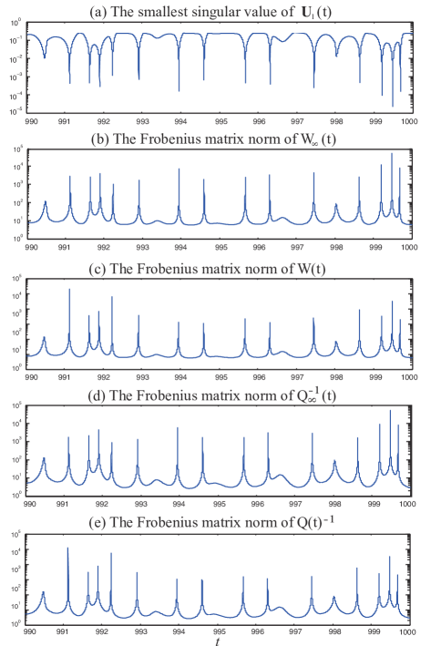
Figure 5: The smallest singular value of $\mathbf{U}_{1}(t)$, $\|W_{\infty}(t)\|_{F}$, $\|W(t)\|_{F}$, $\|Q_{\infty}^{-1}(t)\|_{F}$ and $\|Q(t)^{-1}\|_{F}$ plotted by the log scale.

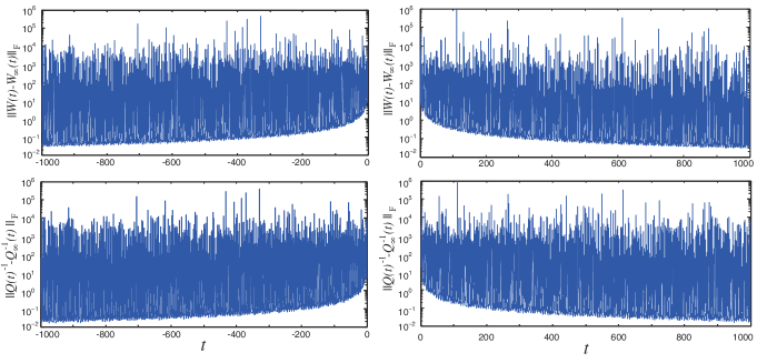
Figure 6: $\|W(t)-W_{\infty}(t)\|_{F}$ and $\|Q(t)^{-1}-Q_{\infty}^{-1}(t)\|_{F}$ plotted by the log scale for $-1000\leqslant t\leqslant 0$ and for $0\leqslant t\leqslant 1000$.

4.4 Application to the Convergence Analysis of SDA

In this subsection, we shall apply the asymptotic analysis of RDE (4.13) studied in previous subsections to the asymptotic behavior of SDA. Throughout this subsection, we fix $(\mathcal{S}_{1},\mathcal{S}_{2})=(I,I)$ (the $\mathbb{S}_{1}$ class) or $(-I,\mathcal{J})$ (the $\mathbb{S}_{2}$ class) and let $X_{1}=[X_{ij}^{1}]_{1\leqslant i,j\leqslant 2}\in{\mathbb{H}}(2n)$ be given such that the pair $(\mathcal{M}_{1},\mathcal{L}_{1})=T_{\mathcal{S}_{1},\mathcal{S}_{2}}(X_{1})\in\mathbb{S}_{1}$ or $\mathbb{S}_{2}$ is regular with ${\rm ind}_{\infty}(\mathcal{M}_{1},\mathcal{L}_{1})\leqslant 1$. Let the idempotent matrices $\Pi_{0}=\Pi_{0}(\mathcal{M}_{1},\mathcal{L}_{1})$, $\Pi_{\infty}=\Pi_{\infty}(\mathcal{M}_{1},\mathcal{L}_{1})$ and the Hamiltonian matrix $\mathcal{H}=\mathcal{H}(\mathcal{M}_{1},\mathcal{L}_{1})$ be defined in Definition 2.2. From Lemma 2.6 it follows that

$$\mathcal{M}_{1}\Pi_{0}=\mathcal{L}_{1}\Pi_{\infty}e^{\mathcal{H}}.$$

Suppose $(\mathcal{M}_{k},\mathcal{L}_{k})$, $k=1,2,\ldots$, is the sequence generated by the SDA and denote $X_{k}=[X^{k}_{ij}]_{1\leq i,j\leq 2}\equiv T_{\mathcal{S}_{1},\mathcal{S}_{2}}^{-1}(\mathcal{M}_{k},\mathcal{L}_{k})$. It is shown in Theorem 3.12 that $X_{k}=X(2^{k-1})$, where $X(t)$ is the extended solution of the IVP (3.26). Therefore, the asymptotic behaviors of the sequence $X_{k}$, as well as the sequence $(\mathcal{M}_{k},\mathcal{L}_{k})$, can be analyzed by using Lemma 4.1 as a connection to what we have studied on the RDE in previous subsections.

Suppose that $\mathcal{S}$ is a symplectic matrix such that $\mathfrak{J}=\mathcal{S}^{-1}\mathcal{H}\mathcal{S}$ has the form in (4.30). Partition $\mathcal{S}$ compatibly with $\mathfrak{J}$ being of the form

$$\mathcal{S}=\left[\begin{array}[]{ccc|ccc}U_{r}&U_{e}&U_{cd}&V_{r}&V_{e}&V_{cd}\end{array}\right]=\left[\begin{array}[]{ccc|ccc}U^{r}_{1}&U^{e}_{1}&U^{cd}_{1}&V^{r}_{1}&V^{e}_{1}&V^{cd}_{1}\\ \hline\cr U^{r}_{2}&U^{e}_{2}&U^{cd}_{2}&V^{r}_{2}&V^{e}_{2}&V^{cd}_{2}\end{array}\right].$$ (4.484)

Let

$$\begin{array}[]{ll}\mathcal{S}_{-}=\mathcal{S}_{2}\mathcal{S},&\mathcal{S}_{+}=\mathcal{J}^{-1}\mathcal{S}_{1}\mathcal{S}\end{array}$$ (4.486)

and

$$\begin{array}[]{rr}\left[\begin{array}[]{c}W_{1}^{-}\\ W_{2}^{-}\\ \end{array}\right]=\mathcal{S}^{-1}\mathcal{S}_{2}^{-1}\left[\begin{array}[]{c}I\\ -X_{22}^{1}\\ \end{array}\right],&\left[\begin{array}[]{c}W_{1}^{+}\\ W_{2}^{+}\\ \end{array}\right]=\mathcal{S}^{-1}\mathcal{S}_{1}^{-1}\mathcal{J}\left[\begin{array}[]{c}I\\ X_{11}^{1}\\ \end{array}\right]\end{array}\in{\mathbb{C}}^{2n\times n}.$$

Partition $W_{j}^{\pm}$ for $j=1,2$ as

$$\begin{array}[]{cc}W_{j}^{\pm}=\left[\begin{array}[]{cc}W^{j,\pm}_{1,1}&W^{j,\pm}_{1,2}\\ W^{j,\pm}_{2,1}&W^{j,\pm}_{2,2}\end{array}\right]&\!\!\!\!\!\!\!\!\begin{array}[]{l}\}n_{r}\\ \}n_{ecd}\end{array}\vspace{-0.3cm}\\ \begin{array}[]{cc}\ \ \ \ \ \ \ \ \ \underbrace{}_{n_{r}}&\ \ \underbrace{}_{n_{ecd}}\end{array}&\end{array}.$$

Here $n_{r}$, $n_{e}$, $n_{c}$ and $n_{d}$ the sizes of $R_{r}$, $R_{e}$, $R_{c}$ and $R_{d}$ in (4.30), respectively. We assume that

Assumption

SDA: $\left[\begin{array}[]{cc}W^{1,+}_{1,1}&W^{1,+}_{1,2}\\ W^{2,+}_{2,1}&W^{2,+}_{2,2}\end{array}\right]$ and $W_{2}^{-}$ are invertible.

From Lemma 4.1, we see that the flows in (4.16) govern the sequence generated by SDA. Under the Assumption SDA, there exist invertible matrices $\mathbf{Z}_{1,\pm}$ in (4.256) such that

$$\left[\begin{array}[]{c}Q(t;\mathcal{S}_{2}\mathcal{H}\mathcal{S}_{2}^{-1},-X_{22}^{1})\\ P(t;\mathcal{S}_{2}\mathcal{H}\mathcal{S}_{2}^{-1},-X_{22}^{1})\\ \end{array}\right]\mathbf{Z}_{1,-}=\mathcal{S}_{-}e^{\mathfrak{J}t}\left[\begin{array}[]{c}\mathbf{W}_{1}^{-}\\ \mathbf{W}_{2}^{-}\\ \end{array}\right],$$ (4.487e)

$$\left[\begin{array}[]{c}Q(t;\widetilde{\mathcal{H}}_{\star},X_{11}^{1})\\ P(t;\widetilde{\mathcal{H}}_{\star},X_{11}^{1})\\ \end{array}\right]\mathbf{Z}_{1,+}=\mathcal{S}_{+}e^{\mathfrak{J}t}\left[\begin{array}[]{c}\mathbf{W}_{1}^{+}\\ \mathbf{W}_{2}^{+}\\ \end{array}\right],$$ (4.487j)

where $\widetilde{\mathcal{H}}_{\star}=\mathcal{J}^{-1}\mathcal{S}_{1}\mathcal{H}\mathcal{S}_{1}^{-1}\mathcal{J}$ and $\mathbf{W}_{1}^{\pm}$, $\mathbf{W}_{2}^{\pm}$ have the form as in (4.262) and $\mathcal{S}_{-}$, $\mathcal{S}_{+}$ are defined in (4.486). The asymptotic behaviors of

$$\begin{array}[]{lll}W(t;\mathcal{S}_{2}\mathcal{H}\mathcal{S}_{2}^{-1},-X_{22}^{1}),&Q(t;\mathcal{S}_{2}\mathcal{H}\mathcal{S}_{2}^{-1},-X_{22}^{1})^{-1},&\text{ as }t\rightarrow-\infty\\ W(t;\widetilde{\mathcal{H}}_{\star},X_{11}^{1}),&Q(t;\widetilde{\mathcal{H}}_{\star},X_{11}^{1})^{-1},&\text{ as }t\rightarrow\infty\end{array}$$

have been studied in Subsection 4.3, and hence, can be used as a fundamental tool for the convergence analysis of SDA.

As a consequence of Lemma 4.1 and Corollary 4.17, we see that the SDA exhibits a quadratic convergence whenever none of nonzero eigenvalues of $\mathcal{H}$ are pure imaginary. A similar convergence analysis has been carried out in [12, 41].

Theorem 4.25.

Suppose that $\mathcal{H}$ has no nonzero pure imaginary eigenvalue, that is, $U_{ecd}$ and $V_{ecd}$ are absent in (4.484) and $\mathfrak{J}=\left[\begin{array}[]{c|c}R_{r}&0\\ \hline\cr 0&-R_{r}^{H}\end{array}\right]$. Let $\mathfrak{r}=\min\{\Re({\rm diag}(R_{r}))\}>0$ and

$$\left[\begin{array}[]{c}\mathscr{U}_{1,-}\\ \mathscr{U}_{2,-}\\ \end{array}\right]=\mathcal{S}_{2}\left[\begin{array}[]{c}V^{r}_{1}\\ V^{r}_{2}\\ \end{array}\right],\ \ \ \ \left[\begin{array}[]{c}\mathscr{U}_{1,+}\\ \mathscr{U}_{2,+}\\ \end{array}\right]=\mathcal{J}^{-1}\mathcal{S}_{1}\left[\begin{array}[]{c}U^{r}_{1}\\ U^{r}_{2}\\ \end{array}\right].$$

If $\mathscr{U}_{1,-}$, $\mathscr{U}_{1,+}$ are invertible and Assumption SDA holds, then

$$\begin{array}[]{ll}X^{k}_{22}=-\mathscr{U}_{2,-}\mathscr{U}_{1,-}^{-1}+O(e^{-\mathfrak{r}2^{k}}2^{2nk}),&X^{k}_{12}=O(e^{-\mathfrak{r}2^{k-1}}2^{nk}),\\ X^{k}_{11}=\mathscr{U}_{2,+}\mathscr{U}_{1,+}^{-1}+O(e^{-\mathfrak{r}2^{k}}2^{2nk}),&X^{k}_{21}=O(e^{-\mathfrak{r}2^{k-1}}2^{nk}),\end{array}$$

as $k\rightarrow\infty$. Here, $\mathscr{U}_{2,-}\mathscr{U}_{1,-}^{-1}$ and $\mathscr{U}_{2,+}\mathscr{U}_{1,+}^{-1}$ are Hermitian.

Proof.

We first prove assertions for $X_{22}^{k}$ and $X_{12}^{k}$. Note that (4.487e) holds due to Assumption SDA. Replacing the matrix $\mathcal{S}$ by $\mathcal{S}_{-}$ in Corollary 4.17, it follows

$$\begin{array}[]{l}W(t;\mathcal{S}_{2}\mathcal{H}\mathcal{S}_{2}^{-1},-X_{22}^{1})=\mathscr{U}_{2,-}\mathscr{U}_{1,-}^{-1}+O(e^{-2\mathfrak{r}|t|}|t|^{2n}),\\ Q(t;\mathcal{S}_{2}\mathcal{H}\mathcal{S}_{2}^{-1},-X_{22}^{1})^{-1}=O(e^{-\mathfrak{r}|t|}|t|^{n}),\end{array}$$

as $t\rightarrow-\infty$. Therefore we conclude from Lemma 4.1 that

$$X^{k}_{22}=-\mathscr{U}_{2,-}\mathscr{U}_{1,-}^{-1}+O(e^{-\mathfrak{r}2^{k}}2^{2nk})\text{ and }X^{k}_{12}=O(e^{-\mathfrak{r}2^{k-1}}2^{nk}),$$

as $k\rightarrow\infty$. Assertions for $X_{11}^{k}$ and $X_{21}^{k}$ can be accordingly obtained by using the matrix $\mathcal{S}_{+}$, (4.487j), Corollary 4.17 and Lemma 4.1. The matrices $\mathscr{U}_{2,-}\mathscr{U}_{1,-}^{-1}$ and $\mathscr{U}_{2,+}\mathscr{U}_{1,+}^{-1}$ are Hermitian because $\mathcal{S}_{-}$ and $\mathcal{S}_{+}$ are symplectic, respectively. ∎

In a similar manner as the proof of Theorem 4.25, the following theorem can be obtained by applying Lemma 4.1 and Corollary 4.20. We see that the SDA exhibits a linear convergence whenever the sizes of Jordan blocks corresponding to nonzero pure imaginary eigenvalues of $\mathcal{H}$ are even. A similar convergence analysis has been proven in [46].

Theorem 4.26.

Suppose that the sizes of Jordan blocks corresponding to nonzero pure imaginary eigenvalues of $\mathcal{H}$ are even, that is, $U_{cd}$ and $V_{cd}$ are absent in (4.484) and $\mathfrak{J}$ has the form in (4.362). Let

$$\left[\begin{array}[]{c}\mathscr{U}_{1,-}\\ \mathscr{U}_{2,-}\\ \end{array}\right]=\mathcal{S}_{2}\left[\begin{array}[]{cc}V^{r}_{1}&U_{1}^{e}\\ V^{r}_{2}&U_{2}^{e}\\ \end{array}\right],\ \ \ \ \left[\begin{array}[]{c}\mathscr{U}_{1,+}\\ \mathscr{U}_{2,+}\\ \end{array}\right]=\mathcal{J}^{-1}\mathcal{S}_{1}\left[\begin{array}[]{cc}U^{r}_{1}&U_{1}^{e}\\ U^{r}_{2}&U_{2}^{e}\\ \end{array}\right].$$

If $\mathscr{U}_{1,-}$, $\mathscr{U}_{1,+}$ are invertible and Assumption SDA holds, then

$$\begin{array}[]{ll}X^{k}_{22}=-\mathscr{U}_{2,-}\mathscr{U}_{1,-}^{-1}+O(2^{-k}),&X^{k}_{12}=O(2^{-k}),\\ X^{k}_{11}=\mathscr{U}_{2,+}\mathscr{U}_{1,+}^{-1}+O(2^{-k}),&X^{k}_{21}=O(2^{-k}),\end{array}$$

as $k\rightarrow\infty$. Here, $\mathscr{U}_{2,-}\mathscr{U}_{1,-}^{-1}$ and $\mathscr{U}_{2,+}\mathscr{U}_{1,+}^{-1}$ are Hermitian.

For the case that the Hamiltonian Jordan canonical form $\mathfrak{J}$ of $\mathcal{H}$ has the form in (4.372), the following theorem can be obtained by applying Lemma 4.1 and Corollary 4.21. We see that the sequences, $X_{22}^{k}$ and $X_{11}^{k}$, converge linearly to constant Hermitian matrices and that the sequences, $X_{12}^{k}$ and $X_{21}^{k}$, tend linearly to closed obits that consist of rank-one matrices.

Theorem 4.27.

Suppose that Assumption SDA holds and the Hamiltonian Jordan canonical form $\mathfrak{J}$ of $\mathcal{H}$ has the form in (4.372), that is, $U_{cd}=U_{c}$ and $V_{cd}=V_{c}$ in (4.484). Let

$$\left[\begin{array}[]{c}\mathscr{U}_{1,-}\\ \mathscr{U}_{2,-}\\ \end{array}\right]=\mathcal{S}_{2}\left[\begin{array}[]{c}\mathbf{U}_{1,-}\\ \mathbf{U}_{2,-}\\ \end{array}\right],\ \ \ \ \left[\begin{array}[]{c}\mathscr{U}_{1,+}\\ \mathscr{U}_{2,+}\\ \end{array}\right]=\mathcal{J}^{-1}\mathcal{S}_{1}\left[\begin{array}[]{c}\mathbf{U}_{1,+}\\ \mathbf{U}_{2,+}\\ \end{array}\right],$$

where $\mathbf{U}_{j,-}$ and $\mathbf{U}_{j,+}$ for $j=1,2$ are defined in (4.373). If $\mathscr{U}_{1,-}$, $\mathscr{U}_{1,+}$ are invertible, then as $k\rightarrow\infty$

$$\begin{array}[]{ll}X^{k}_{22}=-\mathscr{U}_{2,-}\mathscr{U}_{1,-}^{-1}+O(2^{-k}),&X^{k}_{12}=e^{i\eta(2^{k-1}-1)}X^{1}_{12}\mathbf{Z}_{cd,-}^{1}e_{n_{cd}}e_{n}^{H}\mathscr{U}_{1,-}^{-1}+O(2^{-k}),\\ X^{k}_{11}=\mathscr{U}_{2,+}\mathscr{U}_{1,+}^{-1}+O(2^{-k}),&X^{k}_{21}=e^{-i\eta(2^{k-1}-1)}X^{1}_{21}\mathbf{Z}_{cd,+}^{1}e_{n_{cd}}e_{n}^{H}\mathscr{U}_{1,+}^{-1}+O(2^{-k}),\end{array}$$

where $\mathbf{Z}_{cd,\pm}^{1}$ is defined in (4.340). Here, $\mathscr{U}_{2,-}\mathscr{U}_{1,-}^{-1}$ and $\mathscr{U}_{2,+}\mathscr{U}_{1,+}^{-1}$ are Hermitian.

The following theorem can be obtained by applying Lemma 4.1 and Theorem 4.24.

Theorem 4.28.

Suppose that Assumption SDA holds and the Hamiltonian Jordan canonical form $\mathfrak{J}$ of $\mathcal{H}$ is of the form in (4.30). Let

$$\begin{array}[]{ll}\left[\begin{array}[]{c}\mathscr{U}_{1,-}\\ \mathscr{U}_{2,-}\\ \end{array}\right]=\mathcal{S}_{2}\left[\begin{array}[]{c}\mathbf{U}_{1,-}\\ \mathbf{U}_{2,-}\\ \end{array}\right],&\left[\begin{array}[]{c}\Delta\mathscr{U}_{1,-}^{cd}(t)\\ \Delta\mathscr{U}_{2,-}^{cd}(t)\\ \end{array}\right]=\mathcal{S}_{2}\left[\begin{array}[]{c}\Delta\mathbf{U}_{1,-}^{cd}(t)\\ \Delta\mathbf{U}_{2,-}^{cd}(t)\\ \end{array}\right],\\ \left[\begin{array}[]{c}\mathscr{U}_{1,+}\\ \mathscr{U}_{2,+}\\ \end{array}\right]=\mathcal{J}^{-1}\mathcal{S}_{1}\left[\begin{array}[]{c}\mathbf{U}_{1,+}\\ \mathbf{U}_{2,+}\\ \end{array}\right],&\left[\begin{array}[]{c}\Delta\mathscr{U}_{1,+}^{cd}(t)\\ \Delta\mathscr{U}_{2,+}^{cd}(t)\\ \end{array}\right]=\mathcal{J}^{-1}\mathcal{S}_{1}\left[\begin{array}[]{c}\Delta\mathbf{U}_{1,+}^{cd}(t)\\ \Delta\mathbf{U}_{2,+}^{cd}(t)\\ \end{array}\right],\end{array}$$

where $\mathbf{U}_{1,\pm}$, $\mathbf{U}_{2,\pm}$, $\Delta\mathbf{U}_{1,\pm}^{cd}(t)$ and $\Delta\mathbf{U}_{2,\pm}^{cd}(t)$ are defined in (4.478). If $\mathscr{U}_{1,-}$, $\mathscr{U}_{1,+}$ are invertible, then there exist four matrices

$$\mathscr{K}_{W_{\pm}}(k)= \left[\Delta\mathscr{U}^{cd}_{2,\pm}(\pm 2^{k-1}\mp 1)-\mathscr{U}_{2,\pm}\mathscr{U}_{1,\pm}^{-1}\Delta\mathscr{U}^{cd}_{1,\pm}(\pm 2^{k-1}\mp 1)+O(2^{-k})\right]$$

$$[I_{\mu}+\mathsf{E}_{\mu}^{H}\mathscr{U}_{1,\pm}^{-1}\Delta\mathscr{U}^{cd}_{1,\pm}(\pm 2^{k-1}\mp 1)+O(2^{-k})]^{-1}\mathsf{E}_{\mu}^{H}[\mathscr{U}_{1,\pm}^{-1}+O(2^{-k})],$$

$$\mathscr{K}_{Q_{\pm}}(k)= [\mathfrak{Z}_{cd}^{\pm}\Sigma_{\gamma}(\pm 2^{k-1}\mp 1)^{-1}+O(2^{-k})]$$

$$\left[I_{\mu}+\mathsf{E}_{\mu}^{H}\mathscr{U}_{1,\pm}^{-1}\Delta\mathscr{U}^{cd}_{1,\pm}(\pm 2^{k-1}\mp 1)+O(2^{-k})\right]^{-1}\mathsf{E}_{\mu}^{H}[\mathscr{U}_{1,\pm}^{-1}+O(2^{-k})],$$

such that as $k\rightarrow\infty$

$$\begin{array}[]{l}X^{k}_{22}=-\mathscr{U}_{2,-}\mathscr{U}_{1,-}^{-1}-\mathscr{K}_{W_{-}}(k)+O(2^{-k}),\\ X^{k}_{12}=X^{1}_{12}\mathscr{K}_{Q_{-}}(k)+O(2^{-k}),\\ X^{k}_{11}=\mathscr{U}_{2,+}\mathscr{U}_{1,+}^{-1}+\mathscr{K}_{W_{+}}(k)+O(2^{-k}),\\ X^{k}_{21}=X^{1}_{21}\mathscr{K}_{Q_{+}}(k)+O(2^{-k}),\end{array}$$

where $\mathfrak{Z}_{cd}^{\pm},\ \mathsf{E}_{\mu}\in\mathbb{C}^{n\times\mu}$ are defined in (4.446). Here, the ranks of $\mathscr{K}_{W_{\pm}}(k)$ and of $\mathscr{K}_{Q_{\pm}}(k)$ are at most $\mu$, where $\mu$ is the number of Jordan blocks in $R_{cd}$.

A Appendix

A.1 Complementary of Section 2

Let $R>1$, $\theta\in[0,2\pi)$ and

$$D_{R,\theta}=\{z\in\mathbb{C}|1/R\leqslant|z|\leqslant R\}/\{z=re^{i\theta}|\ 1/R\leqslant r\leqslant R\}.$$

Let $\Gamma$ denote the boundary of $D_{R,\theta}$. Suppose that $A\in\mathbb{C}^{n\times n}$ is an invertible matrix and $\sigma(A)\subseteq D_{R,\theta}$. We define Log$(A)$ by

$${\rm Log}(A)=\frac{1}{2\pi i}\oint_{\Gamma}(zI-A)^{-1}(\log z)dz.$$ (A.1)

It has been shown that $e^{{\rm Log}(A)}=A$ for each invertible matrix $A\in\mathbb{C}^{n\times n}$ in [45]. Now, we show that if $\mathcal{S}\in Sp(n)$ then ${\rm Log}(\mathcal{S})$ is Hamiltonian and vice versa.

Theorem A.1.

Suppose that $\mathcal{S}\in Sp(n)$ is symplectic. Then ${\rm Log}(\mathcal{S})$ is Hamiltonian. Conversely, if $\mathcal{H}$ is Hamiltonian, then $e^{\mathcal{H}}$ is symplectic.

Proof.

Since $\mathcal{S}$ is symplectic, then so is $\mathcal{S}^{H}$. Let $\mathcal{S}$ have distinct eigenvalues $\lambda_{1},\ldots,\lambda_{k}$, i.e., $\sigma(\mathcal{S})=\{\lambda_{1},\ldots,\lambda_{k}\}$. Let $R>0$ and $\theta\in[0,2\pi)$ such that $\sigma(\mathcal{S})\cup\sigma(\mathcal{S}^{H})\subseteq D_{R,\theta}$. Since $\mathcal{S}$ is symplectic, we know that for each $\lambda_{j}\in\sigma(\mathcal{S})$, $1/\bar{\lambda}_{j}\in\sigma(\mathcal{S})$. Let $\Gamma_{1},\ldots,\Gamma_{k}\subseteq D_{R,\theta}$ be small nonintersecting circles with positive orientation in the complex plane centered at $\lambda_{1},\ldots,\lambda_{k}$, respectively, which are symmetric with respect to the unit circle. Thus the transformation, $z\rightarrow 1/\bar{z}$, maps the set of circles $\Gamma_{1},\ldots,\Gamma_{k}$ into the set of circles $-\Gamma_{1},\ldots,-\Gamma_{k}$.

From (A.1), we have

$${\rm Log}(\mathcal{S})=\frac{1}{2\pi i}\sum_{j=1}^{k}\oint_{\Gamma_{j}}(zI-\mathcal{S})^{-1}(\log z)dz.$$ (A.2)

Make the change of variable $z=1/\bar{\xi}$ in the integrals in (A.2) and suppose that $\Gamma_{s}\rightarrow-\Gamma_{j}$. Recall that $\mathcal{S}^{-1}=-\mathcal{J}\mathcal{S}^{H}\mathcal{J}$. Then we have

$$\frac{1}{2\pi i}\oint_{\Gamma_{s}}(zI-\mathcal{S})^{-1}(\log z)dz =\frac{1}{2\pi i}\oint_{-\Gamma_{j}}[(1/\bar{\xi})I-\mathcal{S}]^{-1}(-\log\bar{\xi})(-d\bar{\xi}/\bar{\xi}^{2})$$

$$=\frac{-1}{2\pi i}\oint_{\Gamma_{j}}(I-\bar{\xi}\mathcal{S})^{-1}\bar{\xi}^{-1}\log\bar{\xi}d\bar{\xi}$$

$$=\overline{\frac{1}{2\pi i}\oint_{{\Gamma}_{j}}(I-{\xi}\bar{\mathcal{S}})^{-1}{\xi}^{-1}\log{\xi}d{\xi}}$$

$$=\overline{\frac{1}{2\pi i}\oint_{{\Gamma}_{j}}[\bar{\mathcal{S}}(I-{\xi}\bar{\mathcal{S}})^{-1}+{\xi}^{-1}I]\log{\xi}d{\xi}}$$

$$=\overline{\frac{1}{2\pi i}\oint_{{\Gamma}_{j}}[(\bar{\mathcal{S}}^{-1}-{\xi}I)^{-1}+{\xi}^{-1}I]\log{\xi}d{\xi}}$$

$$=\overline{\frac{1}{2\pi i}\oint_{{\Gamma}_{j}}[(-\mathcal{J}\mathcal{S}^{\top}\mathcal{J}+{\xi}\mathcal{J}\mathcal{J})^{-1}+{\xi}^{-1}I]\log{\xi}d{\xi}}$$

$$=\mathcal{J}\overline{\left(\frac{1}{2\pi i}\oint_{{\Gamma}_{j}}({\xi}I-\mathcal{S}^{\top})^{-1}\log{\xi}d{\xi}\right)}\mathcal{J}+\overline{\frac{1}{2\pi i}\oint_{{\Gamma}_{j}}{\xi}^{-1}\log{\xi}d{\xi}}$$

The circle $\Gamma_{j}$ does not enclose the origin, thus $\oint_{\Gamma_{j}}{\xi}^{-1}\log{\xi}d{\xi}=0$. From (A.2) and using the fact that ${\rm Log}(\mathcal{S}^{\top})={\rm Log}(\mathcal{S})^{\top}$, we have ${\rm Log}(\mathcal{S})=\mathcal{J}\overline{{\rm Log}(\mathcal{S})^{\top}}\mathcal{J}=\mathcal{J}{\rm Log}(\mathcal{S})^{H}\mathcal{J}$, and then $\mathcal{J}{\rm Log}(\mathcal{S})=-{\rm Log}(\mathcal{S})^{H}\mathcal{J}$. Therefore, ${\rm Log}(\mathcal{S})$ is Hamiltonian.

For the converse statement, suppose that $\mathcal{H}$ is Hamiltonian, then $-\mathcal{H}^{H}=\mathcal{J}^{-1}\mathcal{H}\mathcal{J}$. By taking the matrix exponential at each sides of the resulting equation, it leads to $e^{\mathcal{H}}\mathcal{J}e^{\mathcal{H}^{H}}=\mathcal{J}$, and hence, $e^{\mathcal{H}}$ is symplectic. ∎

A.2 Complementary of Subsection 4.2

In the following theorem, we show that $\digamma_{k_{1}}^{k_{2}}$ in (4.142) is invertible, where $k_{1}$, $k_{2}$ are positive integers with $0<k_{1}<k_{2}\leqslant 2k_{1}$. In order to prove this, we need a useful formula (Pascal’s law):

$$P^{n}_{r}-P^{n-1}_{r}=rP^{n-1}_{r-1}\ \ \text{ for }n,r\in\mathbb{N}\text{ and }n\geqslant r,$$

where $P^{n}_{r}=n(n-1)\cdots(n-r-1)=\frac{n!}{(n-r)!}$.

Theorem A.2.

Let $k_{1}$, $k_{2}$ be given positive integers satisfying $0<k_{1}<k_{2}\leqslant 2k_{1}$ and $\delta=k_{2}-k_{1}$. Then

$${\rm det}(\digamma_{k_{1}}^{k_{2}})=\frac{\delta!(\delta-1)!\cdots 1!}{k_{2}!(k_{2}-1)!\cdots(k_{1})!},$$

where $\digamma_{k_{1}}^{k_{2}}$ is defined in (4.142). Hence, $\digamma_{k_{1}}^{k_{2}}$ is invertible.

Proof.

Let $D={\rm diag}(k_{2}!,(k_{2}-1)!,\ldots,(k_{1})!)$. Denote

$$\widetilde{\digamma}_{k_{1}}^{k_{2}}\equiv D\digamma_{k_{1}}^{k_{2}}=\left[\begin{array}[]{cccc}P^{k_{2}}_{\delta}&P^{k_{2}}_{\delta-1}&\cdots&P^{k_{2}}_{0}\\ P^{k_{2}-1}_{\delta}&P^{k_{2}-1}_{\delta-1}&\cdots&P^{k_{2}-1}_{0}\\ \vdots&\vdots&&\vdots\\ P^{k_{1}}_{\delta}&P^{k_{1}}_{\delta-1}&\cdots&P^{k_{1}}_{0}\end{array}\right]\in\mathbb{R}^{(\delta+1)\times(\delta+1)}.$$

Let $e_{j}$ be the $j$th column vector of the identity matrix $I_{\delta+1}$ and $E_{i,j}=I_{\delta+1}-e_{i}e_{j}^{H}$. Using Pascal’s law, we have

$$E_{\delta,\delta+1}\cdots E_{2,3}E_{1,2}\widetilde{\digamma}_{k_{1}}^{k_{2}} =\left[\begin{array}[]{ccc|c}\delta P^{k_{2}-1}_{\delta-1}&\cdots&1P^{k_{2}-1}_{0}&0\\ \vdots&\vdots&&\vdots\\ \delta P^{k_{1}}_{\delta-1}&\cdots&1P^{k_{1}}_{0}&0\\ \hline\cr P^{k_{1}}_{\delta}&\cdots&P^{k_{1}}_{1}&1\end{array}\right]$$

$$=\left[\begin{array}[]{c|c}\widetilde{\digamma}_{k_{1}}^{k_{2}-1}&0\\ \hline\cr*&1\end{array}\right]{\rm diag}(\delta,(\delta-1),\cdots,1,1).$$

It is easily seen that ${\rm det}(\widetilde{\digamma}_{k_{1}}^{k_{2}})=\delta!\cdot{\rm det}(\widetilde{\digamma}_{k_{1}}^{k_{2}-1})$. We then have

$${\rm det}(\widetilde{\digamma}_{k_{1}}^{k_{2}}) =\delta!(\delta-1)!\cdots 1!\cdot{\rm det}(\widetilde{\digamma}_{k_{1}}^{k_{1}})$$

$$=\delta!(\delta-1)!\cdots 1!.$$

Hence, we obtain

$${\rm det}(\digamma_{k_{1}}^{k_{2}})=\frac{{\rm det}(\widetilde{\digamma}_{k_{1}}^{k_{2}})}{{\rm det}(D)}=\frac{\delta!(\delta-1)!\cdots 1!}{k_{2}!(k_{2}-1)!\cdots(k_{1})!}.$$

∎

Theorem A.3.

Given $n\in\mathbb{N}$. Let $\kappa_{n}=\widehat{\psi}_{n}^{H}(\widehat{\Gamma}_{n+1}^{2n})^{-1}\phi_{n}$, where $\widehat{\psi}_{n}^{H}=\psi_{n}^{H}P_{n}$, $\phi_{n}$ and $\widehat{\Gamma}_{n+1}^{2n}$ are defined in (4.62). Then

$$\kappa_{n}=\left\{\begin{array}[]{ll}0&\text{ if $n$ is even,}\\ 2&\text{ if $n$ is odd.}\end{array}\right.$$ (A.5)

Proof.

Using the definitions of $\widehat{\psi}_{n}^{H}=\psi_{n}^{H}P_{n}$, $\phi_{n}$ and $\widehat{\Gamma}_{n+1}^{2n}$ in (4.62), it follows from (4.145) that $\kappa_{n}=\mathbf{x}^{H}_{n}(\digamma_{n+1}^{2n})^{-1}\mathbf{y}_{n}$, where $\mathbf{x}_{n}=[1,\frac{1}{2!},\ldots,\frac{1}{n!}]^{H}$, $\mathbf{y}_{n}=[\frac{1}{n!},\frac{1}{(n-1)!},\ldots,1]^{H}$ and $\digamma_{n+1}^{2n}$ is defined in (4.142). It is easily seen that

$$\digamma_{n}^{2n}=\left[\begin{array}[]{cc}\mathbf{y}_{n}&\digamma_{n+1}^{2n}\\ 1&\mathbf{x}_{n}^{H}\end{array}\right].$$

It follows from Theorem A.2 that $\digamma_{n+1}^{2n}$ is invertible. Denote

$$E=\left[\begin{array}[]{c|c}1&0\\ \hline\cr-(\digamma_{n+1}^{2n})^{-1}\mathbf{y}_{n}&I\end{array}\right].$$

Then we have

$$\digamma_{n}^{2n}E=\left[\begin{array}[]{c|c}0&\digamma_{n+1}^{2n}\\ \hline\cr 1-\mathbf{x}_{n}^{H}(\digamma_{n+1}^{2n})^{-1}\mathbf{y}_{n}&\mathbf{x}_{n}^{H}\end{array}\right].$$

From Theorem A.2, we obtain that

$$\frac{n!(n-1)!\cdots 1!}{(2n)!(2n-1)!\cdots n!} ={\rm det}(\digamma_{n}^{2n})={\rm det}(\digamma_{n}^{2n}E)$$

$$=(-1)^{n+2}(1-\kappa_{n}){\rm det}(\digamma_{n+1}^{2n})$$

$$=(-1)^{n}(1-\kappa_{n})\frac{(n-1)!(n-2)!\cdots 1!}{(2n)!(2n-1)!\cdots(n+1)!}.$$

Hence, $(-1)^{n}(1-\kappa_{n})=1$, that is, $\kappa_{n}$ satisfies (A.5). ∎

Lemma A.4.

Let $n\in\mathbb{N}$. Then

• $(\widehat{\Gamma}_{n}^{2n-1})^{-1}\Phi_{n}=O(t^{-1})$, $\widehat{\Phi}_{n}(\widehat{\Gamma}_{n}^{2n-1})^{-1}=O(t^{-1})$ and $\widehat{\Phi}_{n}(\widehat{\Gamma}_{n}^{2n-1})^{-1}\Phi_{n}=O(t^{-1})$ ;

• $\widehat{\Phi}_{n}(\Phi_{n}W\pm\widehat{\Gamma}_{n}^{2n-1})^{-1}=O(t^{-1})$;

as $t\rightarrow\pm\infty$, where $W\in\mathbb{C}^{n\times n}$ is a constant matrix and $\Phi_{n}$, $\widehat{\Gamma}_{n}^{2n-1}$ and $\widehat{\Phi}_{n}$ are given in (4.62).

Proof.

It follows from (4.62) and (4.142) that $(\Xi_{n-1,0})^{-1}=O(1)$, $(\Xi_{0,n-1})^{-1}=O(1)$ and $(\Xi_{n-1,0})^{-1}\Phi_{n}=O(1)$, $\Phi_{n}(\Xi_{0,n-1})^{-1}=O(1)$ as $t\rightarrow\pm\infty$. By using (4.145), we have

$$(\widehat{\Gamma}_{n}^{2n-1})^{-1}\Phi_{n}=t^{-1}P_{n}^{-1}(\Xi_{0,n-1})^{-1}(\digamma_{n}^{2n-1})^{-1}\left[(\Xi_{n-1,0})^{-1}\Phi_{n}\right]=O(t^{-1}),$$

$$\widehat{\Phi}_{n}(\widehat{\Gamma}_{n}^{2n-1})^{-1}=t^{-1}\left[P_{n}^{-1}\Phi_{n}(\Xi_{0,n-1})^{-1}\right](\digamma_{n}^{2n-1})^{-1}(\Xi_{n-1,0})^{-1}=O(t^{-1}),$$

$$\widehat{\Phi}_{n}(\widehat{\Gamma}_{n}^{2n-1})^{-1}\Phi_{n}=t^{-1}\left[P_{n}^{-1}\Phi_{n}(\Xi_{0,n-1})^{-1}\right](\digamma_{n}^{2n-1})^{-1}\left[(\Xi_{n-1,0})^{-1}\Phi_{n}\right]=O(t^{-1}),$$

as $t\rightarrow\pm\infty$. This proves assertion (i). Now, we prove assertion (ii). Note that

$$\widehat{\Phi}_{n}(\Phi_{n}W-\widehat{\Gamma}_{n}^{2n-1})^{-1} =\widehat{\Phi}_{n}\left[(\widehat{\Gamma}_{n}^{2n-1})^{-1}\Phi_{n}W-I\right]^{-1}(\widehat{\Gamma}_{n}^{2n-1})^{-1}.$$

Using the facts in assertion (i), we have

$$\widehat{\Phi}_{n}(\Phi_{n}W-\widehat{\Gamma}_{n}^{2n-1})^{-1} =-\widehat{\Phi}_{n}(\widehat{\Gamma}_{n}^{2n-1})^{-1}-\sum_{k=1}^{\infty}\widehat{\Phi}_{n}\left[(\widehat{\Gamma}_{n}^{2n-1})^{-1}\Phi_{n}W\right]^{k}(\widehat{\Gamma}_{n}^{2n-1})^{-1}$$

$$=O(t^{-1}),$$

as $t\rightarrow\pm\infty$. Similarly, the rest case $\widehat{\Phi}_{n}(\Phi_{n}W+\widehat{\Gamma}_{n}^{2n-1})^{-1}=O(t^{-1})$ can be proven. ∎

Lemma A.5.

Let $n_{1},n_{2}\in\mathbb{N}$. Then, we have

$$\begin{array}[]{ll}(\Upsilon+\widehat{\Gamma}_{n_{1}+1,n_{2}+1}^{2n_{1},2n_{2}})^{-1}=O(t^{-2}),&(\Upsilon+\widehat{\Gamma}_{n_{1}+1,n_{2}+1}^{2n_{1},2n_{2}})^{-1}\phi_{n_{1},n_{2}}^{j}=O(t^{-1}),\\ (\Upsilon+\widehat{\Gamma}_{n_{1}+1,n_{2}+1}^{2n_{1},2n_{2}})^{-1}\Phi_{n_{1},n_{2}}=O(t^{-2}),&\widehat{\psi}_{n_{1},n_{2}}^{j^{H}}(\Upsilon+\widehat{\Gamma}_{n_{1}+1,n_{2}+1}^{2n_{1},2n_{2}})^{-1}=O(t^{-1}),\\ \widehat{\Phi}_{n_{1},n_{2}}(\Upsilon+\widehat{\Gamma}_{n_{1}+1,n_{2}+1}^{2n_{1},2n_{2}})^{-1}=O(t^{-2}),&\widehat{\psi}_{n_{1},n_{2}}^{j^{H}}(\Upsilon+\widehat{\Gamma}_{n_{1}+1,n_{2}+1}^{2n_{1},2n_{2}})^{-1}\Phi_{n_{1},n_{2}}=O(t^{-1}),\\ \widehat{\Phi}_{n_{1},n_{2}}(\Upsilon+\widehat{\Gamma}_{n_{1}+1,n_{2}+1}^{2n_{1},2n_{2}})^{-1}\Phi_{n_{1},n_{2}}=O(t^{-2}),&\widehat{\Phi}_{n_{1},n_{2}}(\Upsilon+\widehat{\Gamma}_{n_{1}+1,n_{2}+1}^{2n_{1},2n_{2}})^{-1}\phi_{n_{1},n_{2}}^{j}=O(t^{-1}),\end{array}$$

as $t\rightarrow\pm\infty$, where $j=1,2$, $\widehat{\Gamma}_{n_{1}+1,n_{2}+1}^{2n_{1},2n_{2}}$, $\Phi_{n_{1},n_{2}}$, $\widehat{\Phi}_{n_{1},n_{2}}$, $\phi_{n_{1},n_{2}}^{j}$ and $\widehat{\psi}_{n_{1},n_{2}}^{j^{H}}$ are defined in (4.101) and $\Upsilon=\Phi_{n_{1},n_{2}}W+\phi^{1}_{n_{1},n_{2}}w^{H}$, $W\in\mathbb{C}^{(n_{1}+n_{2})\times(n_{1}+n_{2})}$ and $w\in\mathbb{C}^{n_{1}+n_{2}}$. Moreover, we also have

$$\widehat{\psi}_{n_{1},n_{2}}^{j^{H}}(\Upsilon+\widehat{\Gamma}_{n_{1}+1,n_{2}+1}^{2n_{1},2n_{2}})^{-1}\phi_{n_{1},n_{2}}^{k}=\widehat{\psi}_{n_{1},n_{2}}^{j^{H}}(\widehat{\Gamma}_{n_{1}+1,n_{2}+1}^{2n_{1},2n_{2}})^{-1}\phi_{n_{1},n_{2}}^{k}+O(t^{-1}),$$

as $t\rightarrow\pm\infty$, where $j,k\in\{1,2\}$.

Proof.

Using the definition of $\widehat{\Gamma}_{n_{1}+1,n_{2}+1}^{2n_{1},2n_{2}}$ in (4.101), it follows from (4.145) that

$$(\widehat{\Gamma}_{n_{1}+1,n_{2}+1}^{2n_{1},2n_{2}})^{-1} =-i\beta\left[-e^{-i\gamma t}P_{n_{1}}^{-1}\left(\Gamma_{n_{1}+1}^{2n_{1}}\right)^{-1}\oplus e^{-i\delta t}P_{n_{2}}^{-1}\left(\Gamma_{n_{2}+1}^{2n_{2}}\right)^{-1}\right]$$

$$=-i\beta t^{-2}\left[-e^{-i\gamma t}P_{n_{1}}^{-1}\left(\Xi_{0,n_{1}-1}\right)^{-1}\left(\digamma_{n_{1}+1}^{2n_{1}}\right)^{-1}\left(\Xi_{n_{1}-1,0}\right)^{-1}\right.$$

$$\ \ \ \ \ \ \ \ \ \ \ \ \ \ \ \left.\oplus e^{-i\delta t}P_{n_{2}}^{-1}\left(\Xi_{0,n_{2}-1}\right)^{-1}\left(\digamma_{n_{2}+1}^{2n_{2}}\right)^{-1}\left(\Xi_{n_{2}-1,0}\right)^{-1}\right].$$

From (4.62), (4.101) and (4.142), we have

$$\begin{array}[]{ll}(\widehat{\Gamma}_{n_{1}+1,n_{2}+1}^{2n_{1},2n_{2}})^{-1}=O(t^{-2}),&(\widehat{\Gamma}_{n_{1}+1,n_{2}+1}^{2n_{1},2n_{2}})^{-1}\phi_{n_{1},n_{2}}^{j}=O(t^{-1}),\\ (\widehat{\Gamma}_{n_{1}+1,n_{2}+1}^{2n_{1},2n_{2}})^{-1}\Phi_{n_{1},n_{2}}=O(t^{-2}),&\widehat{\psi}_{n_{1},n_{2}}^{j^{H}}(\widehat{\Gamma}_{n_{1}+1,n_{2}+1}^{2n_{1},2n_{2}})^{-1}=O(t^{-1}),\\ \widehat{\Phi}_{n_{1},n_{2}}(\widehat{\Gamma}_{n_{1}+1,n_{2}+1}^{2n_{1},2n_{2}})^{-1}=O(t^{-2}),&\widehat{\psi}_{n_{1},n_{2}}^{j^{H}}(\widehat{\Gamma}_{n_{1}+1,n_{2}+1}^{2n_{1},2n_{2}})^{-1}\Phi_{n_{1},n_{2}}=O(t^{-1}),\\ \widehat{\Phi}_{n_{1},n_{2}}(\widehat{\Gamma}_{n_{1}+1,n_{2}+1}^{2n_{1},2n_{2}})^{-1}\Phi_{n_{1},n_{2}}=O(t^{-2}),&\widehat{\Phi}_{n_{1},n_{2}}(\widehat{\Gamma}_{n_{1}+1,n_{2}+1}^{2n_{1},2n_{2}})^{-1}\phi_{n_{1},n_{2}}^{j}=O(t^{-1}),\end{array}$$ (A.10)

as $t\rightarrow\pm\infty$. From (A.10), we have $(\widehat{\Gamma}_{n_{1}+1,n_{2}+1}^{2n_{1},2n_{2}})^{-1}\Upsilon=O(t^{-1})$ as $t\rightarrow\pm\infty$ and then

$$\left(\Upsilon+\widehat{\Gamma}_{n_{1}+1,n_{2}+1}^{2n_{1},2n_{2}}\right)^{-1}=\left(\widehat{\Gamma}_{n_{1}+1,n_{2}+1}^{2n_{1},2n_{2}}\right)^{-1}+\sum_{l=1}^{\infty}(-1)^{l}\left[\left(\widehat{\Gamma}_{n_{1}+1,n_{2}+1}^{2n_{1},2n_{2}}\right)^{-1}\Upsilon\right]^{l}\left(\widehat{\Gamma}_{n_{1}+1,n_{2}+1}^{2n_{1},2n_{2}}\right)^{-1}.$$

Hence, the results of this lemma can be obtained accordingly from (A.10). ∎

A.3 Complementary of Subsection 4.3

Lemma A.6.

When $|t|$ is sufficiently large, the matrix $\mathcal{T}_{e,\pm}$ in (4.353) is invertible and

$$\mathcal{T}_{e,\pm}^{-1}\mathcal{R}_{e}=O(t^{-1}),\ \ \ \mathcal{R}_{e}^{-H}\mathcal{T}_{e,\pm}^{-1}=O(t^{-1}),\ \ \ \mathcal{R}_{e}^{-H}\mathcal{T}_{e,\pm}^{-1}\mathcal{R}_{e}=O(t^{-1}),$$ (A.11)

as $t\rightarrow\pm\infty$.

Proof.

From Theorem 4.8, we have $\mathcal{R}_{e}=\oplus_{j=1}^{k}e^{i\alpha_{j}t}\Phi_{l_{j}}$ and $\mathcal{D}_{e}=-\oplus_{j=1}^{k}e^{i\alpha_{j}t}\beta_{j}^{e}\widehat{\Gamma}_{l_{j}}^{2l_{j}-1}$, where $\Phi_{l_{j}}$ and $\widehat{\Gamma}_{l_{j}}^{2l_{j}-1}$ are defined in (4.62), $\alpha_{j}\in\mathbb{R}$ and $\beta_{j}^{e}\in\{-1,1\}$ for $j=1,\ldots,k$. Since each $\widehat{\Gamma}_{l_{j}}^{2l_{j}-1}$ is invertible, we obtain that $\mathcal{D}_{e}$ is invertible. From Table 1, we have $\mathcal{D}_{e}^{-1}\mathcal{R}_{e}=O(t^{-1})$ as $t\rightarrow\pm\infty$. Therefore, $\mathcal{T}_{e,\pm}=\mathcal{R}_{e}\mathbf{W}^{\pm}_{2,2}+\mathcal{D}_{e}$ is invertible for all sufficiently large values of $|t|$.

It follows from Lemma 4.3 that $\mathcal{R}_{e}^{-H}=\oplus_{j=1}^{k}e^{i\alpha_{j}t}\widehat{\Phi}_{l_{j}}$, where $\widehat{\Phi}_{l_{j}}$ is defined in (4.62). Then using the fact that $\mathcal{T}_{e,\pm}^{-1}=\mathcal{D}_{e}^{-1}+\sum_{k=1}^{\infty}(-1)^{k}[\mathcal{D}_{e}^{-1}\mathcal{R}_{e}\mathbf{W}_{2,2}^{\pm}]^{k}\mathcal{D}_{e}^{-1}$, we obtain (A.11) directly by Table 1. ∎

Lemma A.7.

Let $\mathcal{T}_{e,\pm}$ be the matrix defined in (4.353). Then

$$\begin{array}[]{l}(\mathcal{R}_{cd}\mathbf{W}^{\pm}_{cd}+\mathcal{D}_{cd})^{-1}\mathcal{R}_{cd}\mathbf{W}^{\pm}_{3,2}\mathcal{T}_{e,\pm}^{-1}=O(t^{-1}),\\ (\mathcal{G}_{cd}\mathbf{W}^{\pm}_{cd}+\mathcal{E}_{cd})(\mathcal{R}_{cd}\mathbf{W}^{\pm}_{cd}+\mathcal{D}_{cd})^{-1}\mathcal{R}_{cd}\mathbf{W}^{\pm}_{3,2}\mathcal{T}_{e,\pm}^{-1}=O(t^{-1}),\end{array}$$ (A.14)

as $t\rightarrow\pm\infty$ and $\mathcal{R}_{cd}\mathbf{W}^{\pm}_{cd}+\mathcal{D}_{cd}$ is invertible.

Proof.

From Theorem 4.8 and (4.352), we assume

$$\mathcal{R}_{cd}=\oplus_{\ell=1}^{\mu}\mathbf{B}_{\ell},\ \ \mathcal{D}_{cd}=\oplus_{\ell=1}^{\mu}\mathbf{D}_{\ell},\ \ \mathcal{G}_{cd}=\oplus_{\ell=1}^{\mu}\mathbf{G}_{\ell}\text{ and }\mathcal{E}_{cd}=\oplus_{\ell=1}^{\mu}\mathbf{E}_{\ell},$$ (A.15)

where $\mathbf{B}_{\ell}$, $\mathbf{D}_{\ell}$, $\mathbf{G}_{\ell}$ and $\mathbf{E}_{\ell}$ have the forms in (4.392). It follows from (4.101), (4.142) and (4.145) that

$$\mathbf{D}^{d}_{\ell} =\left[\begin{array}[]{cc}\Xi_{m_{\ell},1}\oplus\Xi_{n_{\ell},1}&0\\ 0&1\end{array}\right]\mathfrak{D}_{\ell}\left[\begin{array}[]{cc}\Xi_{1,m_{\ell}}P_{m_{\ell}}\oplus\Xi_{1,n_{\ell}}P_{n_{\ell}}&0\\ 0&1\end{array}\right],$$

$$=:(\Xi_{m_{\ell},1}^{n_{\ell},1}\oplus 1)\mathfrak{D}_{\ell}(\widehat{\Xi}_{1,m_{\ell}}^{1,n_{\ell}}\oplus 1)$$

where $\mathfrak{D}_{\ell}\equiv\mathfrak{D}_{\ell}(t)=O(1)$ and $\Xi_{j,1}$, $\Xi_{1,j}$ for $j=m_{\ell},n_{\ell}$ are defined in (4.142). Using the definitions of $\mathbf{B}_{\ell}$, $\mathbf{E}_{\ell}$ in (4.392) and equations (4.62), (4.101), yields that

$$(\Xi_{m_{\ell},1}^{n_{\ell},1}\oplus 1)^{-1}\mathbf{B}_{\ell}=O(1),\ \ \ \mathbf{E}_{\ell}(\widehat{\Xi}_{1,m_{\ell}}^{1,n_{\ell}}\oplus 1)^{-1}=O(1).$$ (A.16)

Let $\mathcal{X}_{cd}=\oplus_{\ell=1}^{\mu}(\Xi_{m_{\ell},1}^{n_{\ell},1}\oplus 1)$ and $\widehat{\mathcal{X}}_{cd}=\oplus_{\ell=1}^{\mu}(\widehat{\Xi}_{1,m_{\ell}}^{1,n_{\ell}}\oplus 1)$. Then $\mathcal{X}_{cd}^{-1}\mathcal{R}_{cd}=O(1)$, $\mathcal{E}_{cd}\widehat{\mathcal{X}}_{cd}^{-1}=O(1)$ and $\widehat{\mathcal{X}}_{cd}^{-1}=O(1)$. Since $\mathcal{G}_{cd}=O(1)$, it follows from (A.15) and (A.16) that

$$(\mathcal{G}_{cd}\mathbf{W}^{\pm}_{cd}+\mathcal{E}_{cd})(\mathcal{R}_{cd}\mathbf{W}^{\pm}_{cd}+\mathcal{D}_{cd})^{-1}\mathcal{R}_{cd}\mathbf{W}^{\pm}_{3,2}$$

$$=[\mathcal{G}_{cd}\mathbf{W}^{\pm}_{cd}\widehat{\mathcal{X}}_{cd}^{-1}+\mathcal{E}_{cd}\widehat{\mathcal{X}}_{cd}^{-1}][(\mathcal{X}_{cd}^{-1}\mathcal{R}_{cd})\mathbf{W}^{\pm}_{cd}\widehat{\mathcal{X}}_{cd}^{-1}+\oplus_{\ell=1}^{\mu}\mathfrak{D}_{\ell}]^{-1}(\mathcal{X}_{cd}^{-1}\mathcal{R}_{cd})\mathbf{W}^{\pm}_{3,2}=O(1).$$

From Lemma A.6, we have $\mathcal{T}_{e,\pm}^{-1}=O(t^{-1})$ as $t\rightarrow\pm\infty$. Hence, (A.14) holds. ∎

Proof of Lemma 4.18.

Let $Z_{1,\pm}(t)=\left[\begin{array}[]{cc}\mathcal{T}_{e,\pm}^{-1}&-\mathcal{T}_{e,\pm}^{-1}\mathcal{R}_{e}\mathbf{W}^{\pm}_{2,3}\\ 0&I_{n_{cd}}\end{array}\right]$ for $t\in\mathcal{I}_{\pm}$, where $\mathcal{T}_{e,\pm}$ and $\mathcal{I}_{\pm}$ are defined in (4.353) and (4.354), respectively. Using the fact that $\mathcal{G}_{cd}=O(1)$, it follows form Lemma A.6 that $Z_{1,\pm}(t)=\left[\begin{array}[]{cc}O(t^{-1})&O(t^{-1})\\ 0&I_{n_{cd}}\end{array}\right]$ and

$$\left[\begin{array}[]{cc}\mathcal{R}_{e}\mathbf{W}^{\pm}_{2,2}+\mathcal{D}_{e}&\mathcal{R}_{e}\mathbf{W}^{\pm}_{2,3}\\ \mathcal{R}_{cd}\mathbf{W}^{\pm}_{3,2}&\mathcal{R}_{cd}\mathbf{W}^{\pm}_{cd}+\mathcal{D}_{cd}\\ \hline\cr\mathcal{R}_{e}^{-H}&0\\ \mathcal{G}_{cd}\mathbf{W}^{\pm}_{3,2}&\mathcal{G}_{cd}\mathbf{W}^{\pm}_{cd}+\mathcal{E}_{cd}\end{array}\right]Z_{1,\pm}(t)=\left[\begin{array}[]{cc}I_{n_{e}}&0\\ \mathcal{R}_{cd}\mathbf{W}^{\pm}_{3,2}\mathcal{T}_{e,\pm}^{-1}&\mathcal{R}_{cd}(\mathbf{W}^{\pm}_{cd}+O(t^{-1}))+\mathcal{D}_{cd}\\ \hline\cr O(t^{-1})&O(t^{-1})\\ O(t^{-1})&\mathcal{G}_{cd}(\mathbf{W}^{\pm}_{cd}+O(t^{-1}))+\mathcal{E}_{cd}\end{array}\right],$$ (A.25)

as $t\rightarrow\pm\infty$. We know that $\mathcal{R}_{cd}(\mathbf{W}^{\pm}_{cd}+O(t^{-1}))+\mathcal{D}_{cd}$ is invertible for $t\in\mathcal{I}_{\pm}$. Let

$$Z_{2,\pm}(t)=\left[\begin{array}[]{cc}I_{n_{e}}&0\\ -(\mathcal{R}_{cd}(\mathbf{W}^{\pm}_{cd}+O(t^{-1}))+\mathcal{D}_{cd})^{-1}\mathcal{R}_{cd}\mathbf{W}^{\pm}_{3,2}\mathcal{T}_{e,\pm}^{-1}&I_{n_{cd}}\end{array}\right],$$

for $t\in\mathcal{I}_{\pm}$. Since $\mathbf{W}^{\pm}_{cd}+O(t^{-1})=O(1)$, the consequences of Lemma A.7 also hold true whenever the matrix $\mathbf{W}_{cd}^{\pm}$ in the statement is replaced by any $O(1)$ matrix. Hence, from Lemma A.7, we have $Z_{2,\pm}(t)=\left[\begin{array}[]{cc}I_{n_{e}}&0\\ O(t^{-1})&I_{n_{cd}}\end{array}\right]$, as $t\rightarrow\pm\infty$. Denote $Z_{ecd,\pm}(t)=Z_{1,\pm}(t)Z_{2,\pm}(t)$ for $t\in\mathcal{I}_{\pm}$. It is easily seen that the asymptotic behavior of $Z_{ecd,\pm}(t)$ has the form (4.355f). Substituting (4.345) into (4.325), it follows from (A.25) that we obtain (4.355k) as $t\rightarrow\pm\infty$. ∎

Proof of Lemma 4.22.

Let $Y(t)\equiv\left[\begin{array}[]{c}Q(t)\\ \hline\cr P(t)\end{array}\right]=\left[\begin{array}[]{c|c}\mathcal{R}_{cd}&\mathcal{D}_{cd}\\ \hline\cr\mathcal{G}_{cd}&\mathcal{E}_{cd}\end{array}\right]\left[\begin{array}[]{c}\mathbf{W}\\ \hline\cr I\end{array}\right]$. From (4.398) and (4.405), we have

$$\left[\begin{array}[]{c}Q(t)\\ \hline\cr P(t)\end{array}\right]=\left[\begin{array}[]{cc}\mathbf{B}_{1}\mathbf{W}_{11}+\mathbf{D}_{1}&\mathbf{B}_{1}\mathbf{W}_{12}\\ \mathbf{B}_{2}\mathbf{W}_{21}&\mathbf{B}_{2}\mathbf{W}_{22}+\mathbf{D}_{2}\\ \hline\cr\mathbf{G}_{1}\mathbf{W}_{11}+\mathbf{E}_{1}&\mathbf{G}_{1}\mathbf{W}_{12}\\ \mathbf{G}_{2}\mathbf{W}_{21}&\mathbf{G}_{2}\mathbf{W}_{22}+\mathbf{E}_{2}\end{array}\right].$$ (A.32)

Partition $\mathbf{W}_{jk}$ as $\mathbf{W}_{jk}=\left[\begin{array}[]{cc}\mathbf{W}^{jk}_{11}&\mathbf{w}^{jk}_{12}\\ \mathbf{w}^{jk}_{21}&\mathbf{w}^{jk}_{22}\end{array}\right]$, where $\mathbf{w}^{jk}_{22}=\mathbf{w}_{jk}:=\mathbf{W}_{jk}(\varkappa_{j},\varkappa_{k})\in\mathbb{C}$, for $j,k\in\{1,2\}$ and denote $\mathbf{B}_{j}\equiv\left[\begin{array}[]{c}\mathbf{B}^{j}_{1}\\ \hline\cr\mathbf{b}^{j}_{2}\end{array}\right]:=\left[\begin{array}[]{cc}\Phi_{m_{j},n_{j}}&\phi_{m_{j},n_{j}}^{1}\\ \hline\cr 0&\omega_{11}^{j}\end{array}\right]$, for $j=1,2$. Let

$$\begin{array}[]{l}\Upsilon_{1}=\Phi_{m_{1},n_{1}}\mathbf{W}^{11}_{11}+\phi_{m_{1},n_{1}}^{1}\mathbf{w}^{11}_{21},\\ p_{1}=\Phi_{m_{1},n_{1}}\mathbf{w}^{11}_{12}+\phi_{m_{1},n_{1}}^{1}\mathbf{w}^{11}_{22}+\phi_{m_{1},n_{1}}^{2},\\ \Omega_{11}(t)=\left[\begin{array}[]{c|c}\left(\Upsilon_{1}+\widehat{\Gamma}_{m_{1}+1,n_{1}+1}^{2m_{1},2n_{1}}\right)^{-1}&-\left(\Upsilon_{1}+\widehat{\Gamma}_{m_{1}+1,n_{1}+1}^{2m_{1},2n_{1}}\right)^{-1}p_{1}\\ \hline\cr 0&1\end{array}\right],\\ \Omega_{1}(t)=\left[\begin{array}[]{c|c}\Omega_{11}(t)&\left[\begin{array}[]{c}-\left(\Upsilon_{1}+\widehat{\Gamma}_{m_{1}+1,n_{1}+1}^{2m_{1},2n_{1}}\right)^{-1}\mathbf{B}^{1}_{1}\mathbf{W}_{12}\\ 0\end{array}\right]\\ \hline\cr 0&I_{\varkappa_{2}}\end{array}\right],\\ \zeta^{1}_{jk}=\widehat{\psi}_{m_{1},n_{1}}^{j^{H}}\left(\widehat{\Gamma}_{m_{1}+1,n_{1}+1}^{2m_{1},2n_{1}}\right)^{-1}\phi_{m_{1},n_{1}}^{k},\ \ \text{for }j,k\in\{1,2\}.\end{array}$$ (A.44)

From Table 2, we have

$$\begin{array}[]{l}\Omega_{11}(t)=\left[\begin{array}[]{c|c}O(t^{-2})&O(t^{-1})\\ \hline\cr 0&1\end{array}\right],\ \ \Omega_{1}(t)=\left[\begin{array}[]{c|c}O(1)&O(t^{-1})\\ \hline\cr 0&I_{\varkappa_{2}}\end{array}\right],\\ \widehat{\Phi}_{m_{1},n_{1}}\left(\Upsilon_{1}+\widehat{\Gamma}_{m_{1}+1,n_{1}+1}^{2m_{1},2n_{1}}\right)^{-1}\mathbf{B}^{1}_{1}\mathbf{W}_{12}=O(t^{-1}),\\ \widehat{\psi}_{m_{1},n_{1}}^{1^{H}}\left(\Upsilon_{1}+\widehat{\Gamma}_{m_{1}+1,n_{1}+1}^{2m_{1},2n_{1}}\right)^{-1}\mathbf{B}^{1}_{1}\mathbf{W}_{12}=\zeta^{1}_{11}[\mathbf{w}^{12}_{21},\mathbf{w}^{12}_{22}]+O(t^{-1}),\\ \widehat{\psi}_{m_{1},n_{1}}^{2^{H}}\left(\Upsilon_{1}+\widehat{\Gamma}_{m_{1}+1,n_{1}+1}^{2m_{1},2n_{1}}\right)^{-1}\mathbf{B}^{1}_{1}\mathbf{W}_{12}=\zeta^{1}_{21}[\mathbf{w}^{12}_{21},\mathbf{w}^{12}_{22}]+O(t^{-1}),\end{array}$$ (A.53)

as $t\rightarrow\pm\infty$, where $\zeta^{1}_{11}$ and $\zeta^{1}_{21}$ are defined in (A.44). Post multiplying $\Omega_{1}(t)$ to (A.32), it follows from (A.44) and (A.53) that, as $t\rightarrow\pm\infty$,

$$Q(t)\Omega_{1}(t) =\left[\begin{array}[]{c|c}\mathbf{B}_{1}\mathbf{W}_{11}+\mathbf{D}_{1}&\mathbf{B}_{1}\mathbf{W}_{12}\\ \hline\cr\mathbf{B}_{2}\mathbf{W}_{21}&\mathbf{B}_{2}\mathbf{W}_{22}+\mathbf{D}_{2}\end{array}\right]\Omega_{1}(t)$$ (A.54c)

$$=\left[\begin{array}[]{c|c}\begin{array}[]{cc}I&0\\ O(t^{-1})&\varpi^{u}_{11}\end{array}&\begin{array}[]{c}0\\ (\omega_{11}^{1}-\zeta^{1}_{11})[\mathbf{w}^{12}_{21},\mathbf{w}^{12}_{22}]+O(t^{-1})\end{array}\\ \hline\cr\mathbf{B}_{2}\mathbf{W}_{21}\Omega_{11}(t)&\mathbf{B}_{2}(\mathbf{W}_{22}+\Delta)+\mathbf{D}_{2}\end{array}\right],$$ (A.54j)

$$P(t)\Omega_{1}(t) =\left[\begin{array}[]{c|c}\mathbf{G}_{1}\mathbf{W}_{11}+\mathbf{E}_{1}&\mathbf{G}_{1}\mathbf{W}_{12}\\ \hline\cr\mathbf{G}_{2}\mathbf{W}_{21}&\mathbf{G}_{2}\mathbf{W}_{22}+\mathbf{E}_{2}\end{array}\right]\Omega_{1}(t)$$ (A.54m)

$$=\left[\begin{array}[]{c|c}\begin{array}[]{cc}0&0\\ 0&\varpi^{d}_{11}\end{array}&\begin{array}[]{c}0\\ (\omega_{21}^{1}-\zeta^{1}_{21})[\mathbf{w}^{12}_{21},\mathbf{w}^{12}_{22}]\end{array}\\ \hline\cr\mathbf{G}_{2}\mathbf{W}_{21}\Omega_{11}(t)&\mathbf{G}_{2}(\mathbf{W}_{22}+\Delta)+\mathbf{E}_{2}\end{array}\right]+\left[\begin{array}[]{c}O(t^{-1})\\ \hline\cr 0\end{array}\right],$$ (A.54v)

where $\omega_{11}^{1}-\zeta^{1}_{11}=O(1)$, $\omega_{21}^{1}-\zeta^{1}_{21}=O(1)$, $\Delta=\mathbf{W}_{21}\left[\begin{array}[]{c}-\left(\Upsilon_{1}+\widehat{\Gamma}_{m_{1}+1,n_{1}+1}^{2m_{1},2n_{1}}\right)^{-1}\mathbf{B}^{1}_{1}\mathbf{W}_{12}\\ 0\end{array}\right]$ and

$$\left[\begin{array}[]{c}\varpi^{u}_{11}\\ \hline\cr\varpi^{d}_{11}\end{array}\right] =\left[\begin{array}[]{cc}\omega^{1}_{11}&\omega^{1}_{12}\\ \hline\cr\omega^{1}_{21}&\omega^{1}_{22}\end{array}\right]\left[\begin{array}[]{c}\mathbf{w}^{11}_{22}\\ 1\end{array}\right]-\left[\begin{array}[]{c}\zeta^{1}_{11}\mathbf{w}^{11}_{22}+\zeta^{1}_{12}\\ \hline\cr\zeta^{1}_{21}\mathbf{w}^{11}_{22}+\zeta^{1}_{22}\end{array}\right]$$

$$=\left[\begin{array}[]{cc}\omega^{1}_{11}-\zeta^{1}_{11}&\omega^{1}_{12}-\zeta^{1}_{12}\\ \hline\cr\omega^{1}_{21}-\zeta^{1}_{21}&\omega^{1}_{22}-\zeta^{1}_{22}\end{array}\right]\left[\begin{array}[]{c}\mathbf{w}^{11}_{22}\\ 1\end{array}\right].$$

From (A.53), we have $\Delta=O(t^{-1})$ as $t\rightarrow\pm\infty$. Let $\widetilde{\mathbf{W}}_{22}=\mathbf{W}_{22}+\Delta$. Then

$$\widetilde{\mathbf{W}}_{22}=\left[\begin{array}[]{cc}\widetilde{\mathbf{W}}^{22}_{11}&\widetilde{\mathbf{w}}^{22}_{12}\\ \widetilde{\mathbf{w}}^{22}_{21}&\widetilde{\mathbf{w}}^{22}_{22}\end{array}\right]=\left[\begin{array}[]{cc}\mathbf{W}^{22}_{11}&\mathbf{w}^{22}_{12}\\ \mathbf{w}^{22}_{21}&\mathbf{w}^{22}_{22}\end{array}\right]+O(t^{-1}).$$

Similarly, let $\Upsilon_{2}=\Phi_{m_{2},n_{2}}\widetilde{\mathbf{W}}^{22}_{11}+\phi_{m_{2},n_{2}}^{1}\widetilde{\mathbf{w}}^{22}_{21}$, $p_{2}=\Phi_{m_{2},n_{2}}\widetilde{\mathbf{w}}^{22}_{12}+\phi_{m_{2},n_{2}}^{1}\widetilde{\mathbf{w}}^{22}_{22}+\phi_{m_{2},n_{2}}^{2},$

$$\begin{array}[]{l}\Omega_{22}(t)=\left[\begin{array}[]{c|c}\left(\Upsilon_{2}+\widehat{\Gamma}_{m_{2}+1,n_{2}+1}^{2m_{2},2n_{2}}\right)^{-1}&-\left(\Upsilon_{2}+\widehat{\Gamma}_{m_{2}+1,n_{2}+1}^{2m_{2},2n_{2}}\right)^{-1}p_{2}\\ \hline\cr 0&1\end{array}\right],\\ \Omega_{2}(t)=\left[\begin{array}[]{c|c}I_{\varkappa_{1}}&0\\ \hline\cr\left[\begin{array}[]{c}-\left(\Upsilon_{2}+\widehat{\Gamma}_{m_{2}+1,n_{2}+1}^{2m_{2},2n_{2}}\right)^{-1}\mathbf{B}^{2}_{1}\mathbf{W}_{21}\Omega_{11}(t)\\ 0\end{array}\right]&\Omega_{22}(t)\end{array}\right],\\ \zeta^{2}_{jk}=\widehat{\psi}_{m_{2},n_{2}}^{j^{H}}\left(\widehat{\Gamma}_{m_{2}+1,n_{2}+1}^{2m_{2},2n_{2}}\right)^{-1}\phi_{m_{2},n_{2}}^{k},\ \ \text{for }j,k\in\{1,2\}.\end{array}$$ (A.64)

Then $\Omega_{22}(t)=\left[\begin{array}[]{c|c}O(t^{-2})&O(t^{-1})\\ \hline\cr 0&1\end{array}\right]$ and $\Omega_{2}(t)=\left[\begin{array}[]{c|c}I_{\varkappa_{1}}&0\\ \hline\cr O(t^{-1})&O(1)\end{array}\right]$, as $t\rightarrow\pm\infty$. Denote $\Omega(t)=\Omega_{1}(t)\Omega_{2}(t)$. From (A.53) and (A.64), we have

$$\Omega(t)=\left[\begin{array}[]{c|c}e_{\varkappa_{1}}e_{\varkappa_{1}}^{H}&0\\ \hline\cr 0&e_{\varkappa_{2}}e_{\varkappa_{2}}^{H}\end{array}\right]+O(t^{-1}),\text{ as }t\rightarrow\pm\infty.$$

Using the fact that $\omega_{11}^{1}-\zeta^{1}_{11}=O(1)$, $\omega_{21}^{1}-\zeta^{1}_{21}=O(1)$ and from (A.54) and Table 2, we have

$$\begin{array}[]{l}Q(t)\Omega(t)=\left[\begin{array}[]{cc|cc}I&0&0&0\\ 0&\varpi^{u}_{11}&0&(\omega_{11}^{1}-\zeta^{1}_{11})\mathbf{w}^{12}_{22}\\ \hline\cr 0&0&I&0\\ 0&(\omega_{11}^{2}-\zeta^{2}_{11})\mathbf{w}^{21}_{22}&0&\varpi^{u}_{22}\end{array}\right]+O(t^{-1}),\\ P(t)\Omega(t)=\left[\begin{array}[]{cc|cc}0&0&0&0\\ 0&\varpi^{d}_{11}&0&(\omega_{21}^{1}-\zeta^{1}_{21})\mathbf{w}^{12}_{22}\\ \hline\cr 0&0&0&0\\ 0&(\omega_{21}^{2}-\zeta^{2}_{21})\mathbf{w}^{21}_{22}&0&\varpi^{d}_{22}\end{array}\right]+O(t^{-1}),\\ \left[\begin{array}[]{c}\varpi^{u}_{22}\\ \hline\cr\varpi^{d}_{22}\end{array}\right]=\left[\begin{array}[]{cc}\omega^{2}_{11}-\zeta^{2}_{11}&\omega^{2}_{12}-\zeta^{2}_{12}\\ \hline\cr\omega^{2}_{21}-\zeta^{2}_{21}&\omega^{2}_{22}-\zeta^{2}_{22}\end{array}\right]\left[\begin{array}[]{c}\mathbf{w}^{22}_{22}\\ 1\end{array}\right]+O(t^{-1}),\end{array}$$ (A.82)

as $t\rightarrow\pm\infty$. Note that $\mathbf{w}^{jk}_{22}=\mathbf{w}_{jk}:=\mathbf{W}_{jk}(\varkappa_{j},\varkappa_{k})$ for each $j,k\in\{1,2\}$.

From the definitions of $\zeta^{\ell}_{jk}$, for $\ell,j,k\in\{1,2\}$, in (A.44) and (A.64), we have

$$\left[\begin{array}[]{cc}\zeta^{\ell}_{11}&\zeta^{\ell}_{12}\\ \zeta^{\ell}_{21}&\zeta^{\ell}_{22}\end{array}\right]=\Theta^{H}\left[\begin{array}[]{c|c}\widehat{\psi}_{m_{\ell}}^{H}&0\\ \hline\cr 0&\widehat{\psi}_{n_{\ell}}^{H}\end{array}\right]\left[\begin{array}[]{c|c}\widehat{\Gamma}_{m_{\ell}+1}^{2m_{\ell}}&0\\ \hline\cr 0&\widehat{\Gamma}_{n_{\ell}+1}^{2n_{\ell}}\end{array}\right]^{-1}\left[\begin{array}[]{c|c}e^{i\gamma_{\ell}t}\phi_{m_{\ell}}&0\\ \hline\cr 0&e^{i\delta_{\ell}t}\phi_{n_{\ell}}\end{array}\right]\Theta,$$

where $\Theta$ in (4.184) is unitary. From Theorem A.3, we obtain that

$$\left[\begin{array}[]{cc}\zeta^{\ell}_{11}&\zeta^{\ell}_{12}\\ \zeta^{\ell}_{21}&\zeta^{\ell}_{22}\end{array}\right] =\Theta^{H}\left[\begin{array}[]{cc}\kappa_{m_{\ell}}&0\\ 0&\kappa_{n_{\ell}}\end{array}\right]\left[\begin{array}[]{cc}e^{i\gamma_{\ell}t}&0\\ 0&e^{i\delta_{\ell}t}\end{array}\right]\Theta$$

$$=\frac{1}{2}\left[\begin{array}[]{cc}\kappa_{m_{\ell}}e^{i\gamma_{\ell}t}+\kappa_{n_{\ell}}e^{i\delta_{\ell}t}&-i\beta^{d}_{\ell}(\kappa_{m_{\ell}}e^{i\gamma_{\ell}t}-\kappa_{n_{\ell}}e^{i\delta_{\ell}t})\\ i\beta^{d}_{\ell}(\kappa_{m_{\ell}}e^{i\gamma_{\ell}t}-\kappa_{n_{\ell}}e^{i\delta_{\ell}t})&\kappa_{m_{\ell}}e^{i\gamma_{\ell}t}+\kappa_{n_{\ell}}e^{i\delta_{\ell}t}\end{array}\right],$$

where $\kappa_{m_{\ell}}$ and $\kappa_{n_{\ell}}$ satisfy (A.5). Using the definitions $\omega^{\ell}_{jk}$, for $\ell,j,k\in\{1,2\}$, in (4.101) yields that

$$\left[\begin{array}[]{cc}\hat{\omega}^{\ell}_{11}&\hat{\omega}^{\ell}_{12}\\ \hat{\omega}^{\ell}_{21}&\hat{\omega}^{\ell}_{22}\end{array}\right] \equiv\left[\begin{array}[]{cc}\omega^{\ell}_{11}-\zeta^{\ell}_{11}&\omega^{\ell}_{12}-\zeta^{\ell}_{12}\\ \omega^{\ell}_{21}-\zeta^{\ell}_{21}&\omega^{\ell}_{22}-\zeta^{\ell}_{22}\end{array}\right]$$

$$= \frac{1}{2}\left[\begin{array}[]{cc}(-1)^{m_{\ell}}e^{i\gamma_{\ell}t}+(-1)^{n_{\ell}}e^{i\delta_{\ell}t}&-i\beta^{d}_{\ell}((-1)^{m_{\ell}}e^{i\gamma_{\ell}t}-(-1)^{n_{\ell}}e^{i\delta_{\ell}t})\\ i\beta^{d}_{\ell}((-1)^{m_{\ell}}e^{i\gamma_{\ell}t}-(-1)^{n_{\ell}}e^{i\delta_{\ell}t})&(-1)^{m_{\ell}}e^{i\gamma_{\ell}t}+(-1)^{n_{\ell}}e^{i\delta_{\ell}t}\end{array}\right].$$

From (A.32) and (A.82), there exists an invertible matrix $\Omega(t)$ such that (4.418) holds. ∎

Proof of Theorem 4.24.

Form (4.460) and (4.473), we have $\Delta_{u}^{\pm}(t)=\Sigma_{\hat{\omega}_{11}}\mathfrak{W}_{cd}^{\pm}+\Sigma_{\hat{\omega}_{12}}$, $\Delta_{v}^{\pm}(t)=\Sigma_{\hat{\omega}_{21}}\mathfrak{W}_{cd}^{\pm}+\Sigma_{\hat{\omega}_{22}}$ and $\Sigma_{\beta^{cd}}\Sigma_{\beta^{cd}}=I$. From (4.397), (4.446) and (4.460), we have

$$\mathfrak{U}_{cd}\Delta_{\pm}(t) =\mathfrak{U}^{cd}_{u}(\Sigma_{\hat{\omega}_{11}}\mathfrak{W}_{cd}^{\pm}+\Sigma_{\hat{\omega}_{12}})+\mathfrak{U}^{cd}_{v}(\Sigma_{\hat{\omega}_{21}}\mathfrak{W}_{cd}^{\pm}+\Sigma_{\hat{\omega}_{22}})$$

$$=\mathfrak{U}^{cd}_{u}\Sigma_{\hat{\omega}_{11}}\mathfrak{W}_{cd}^{\pm}+\mathfrak{U}^{cd}_{u}(i\Sigma_{\beta^{cd}})(-i\Sigma_{\beta^{cd}})\Sigma_{\hat{\omega}_{12}}+\mathfrak{U}^{cd}_{v}(\Sigma_{\hat{\omega}_{21}}\mathfrak{W}_{cd}^{\pm}+\Sigma_{\hat{\omega}_{22}})$$

$$=[\mathfrak{U}^{cd}_{u}\Sigma_{\hat{\omega}_{11}}+\mathfrak{U}^{cd}_{v}\Sigma_{\hat{\omega}_{21}}]\mathfrak{W}_{cd}^{\pm}+\frac{i}{2}\mathfrak{U}^{cd}_{u}\Sigma_{\beta^{cd}}(-\Sigma_{\gamma}+\Sigma_{\delta})+\frac{1}{2}\mathfrak{U}^{cd}_{v}(\Sigma_{\gamma}+\Sigma_{\delta})$$

$$=[\mathfrak{U}^{cd}_{u}\Sigma_{\hat{\omega}_{11}}+\mathfrak{U}^{cd}_{v}\Sigma_{\hat{\omega}_{21}}]\mathfrak{W}_{cd}^{\pm}+\frac{1}{2}[\mathfrak{U}^{cd}_{v}-i\mathfrak{U}^{cd}_{u}\Sigma_{\beta^{cd}}]\Sigma_{\gamma}+\frac{1}{2}[\mathfrak{U}^{cd}_{v}+i\mathfrak{U}^{cd}_{u}\Sigma_{\beta^{cd}}]\Sigma_{\delta}.$$

Since $\Sigma_{\gamma}$ is invertible, we obtain

$$\mathfrak{U}_{cd}\Delta_{\pm}(t)\Sigma_{\gamma}^{-1}= \frac{1}{2}[\mathfrak{U}^{cd}_{v}-i\mathfrak{U}^{cd}_{u}\Sigma_{\beta^{cd}}]+[\mathfrak{U}^{cd}_{u}\Sigma_{\hat{\omega}_{11}}+\mathfrak{U}^{cd}_{v}\Sigma_{\hat{\omega}_{21}}]\mathfrak{W}_{cd}^{\pm}\Sigma_{\gamma}^{-1}$$

$$+\frac{1}{2}[\mathfrak{U}^{cd}_{v}+i\mathfrak{U}^{cd}_{u}\Sigma_{\beta^{cd}}]\Sigma_{\delta}\Sigma_{\gamma}^{-1}.$$

From (4.464) and (4.465), there exists an invertible matrix $\mathbf{Z}_{\pm}(t)$ such that

$$Y(t)\mathbf{Z}_{\pm}(t)(I_{n-\mu}\oplus\Sigma_{\gamma}^{-1})=\left[\begin{array}[]{c}\mathbf{U}_{1,\pm}+\Delta\mathbf{U}_{1,\pm}(t)\\ \mathbf{U}_{2,\pm}+\Delta\mathbf{U}_{2,\pm}(t)\end{array}\right]+O(t^{-1}),$$ (A.85)

as $t\rightarrow\pm\infty$, where for $j=1,2$, $\Delta\mathbf{U}_{j,\pm}(t)\equiv\left[0,\Delta\mathbf{U}^{cd}_{j,\pm}(t)\right]=\Delta\mathbf{U}^{cd}_{j,\pm}(t)\mathsf{E}_{\mu}^{H}$ and $\mathsf{E}_{\mu}$ and $\Delta\mathbf{U}^{cd}_{j,\pm}(t)$ are defined in (4.446) and (4.478), respectively. It follows from the definition of $W(t)$ and (A.85) that there are matrix functions, $M^{\varepsilon}_{1}(t)=O(t^{-1})$ and $M^{\varepsilon}_{2}(t)=O(t^{-1})$ as $t\rightarrow\pm\infty$, such that

$$W(t) =P(t)Q(t)^{-1}=(\mathbf{U}_{2,\pm}+\Delta\mathbf{U}_{2,\pm}(t)+M^{\varepsilon}_{2}(t))(\mathbf{U}_{1,\pm}+\Delta\mathbf{U}_{1,\pm}(t)+M^{\varepsilon}_{1}(t))^{-1}$$

$$=\left(\mathbf{U}_{2,\pm}+\Delta\mathbf{U}^{cd}_{2,\pm}(t)\mathsf{E}_{\mu}^{H}\right)\left[(\mathbf{U}_{1,\pm}+M^{\varepsilon}_{1}(t))+\Delta\mathbf{U}^{cd}_{1,\pm}(t)\mathsf{E}_{\mu}^{H}\right]^{-1}$$

$$\ \ \ \ +M^{\varepsilon}_{2}(t)\left[(\mathbf{U}_{1,\pm}+M^{\varepsilon}_{1}(t))+\Delta\mathbf{U}^{cd}_{1,\pm}(t)\mathsf{E}_{\mu}^{H}\right]^{-1}.$$ (A.86)

We assume that $\mathbf{U}^{\varepsilon}_{1,\pm}(t)\equiv\mathbf{U}_{1,\pm}+M^{\varepsilon}_{1}(t)$ is invertible. Applying the Sherman-Morrison-Woodbury formula, we have

$$( \mathbf{U}^{\varepsilon}_{1,\pm}(t)+\Delta\mathbf{U}^{cd}_{1,\pm}(t)\mathsf{E}_{\mu}^{H})^{-1}=\mathbf{U}^{\varepsilon}_{1,\pm}(t)^{-1}$$

$$\hskip 28.45274pt-\mathbf{U}^{\varepsilon}_{1,\pm}(t)^{-1}\Delta\mathbf{U}^{cd}_{1,\pm}(t)(I_{\mu}+\mathsf{E}_{\mu}^{H}\mathbf{U}^{\varepsilon}_{1,\pm}(t)^{-1}\Delta\mathbf{U}^{cd}_{1,\pm}(t))^{-1}\mathsf{E}_{\mu}^{H}\mathbf{U}^{\varepsilon}_{1,\pm}(t)^{-1}.$$ (A.87)

Since $\mathbf{U}_{1,\pm}$ is invertible and $M^{\varepsilon}_{1}(t)=O(t^{-1})$ as $t\rightarrow\pm\infty$, we see that

$$\mathbf{U}^{\varepsilon}_{1,\pm}(t)^{-1}=(\mathbf{U}_{1,\pm}+M^{\varepsilon}_{1}(t))^{-1}=\mathbf{U}_{1,\pm}^{-1}+O(t^{-1}),$$ (A.88)

as $t\rightarrow\pm\infty$. Substituting (A.3) and (A.88) into (A.86), it turns out

$$W(t) =\mathbf{U}_{2,\pm}\mathbf{U}^{\varepsilon}_{1,\pm}(t)^{-1}+\Delta\mathbf{U}^{cd}_{2,\pm}(t)\mathsf{E}_{\mu}^{H}\mathbf{U}^{\varepsilon}_{1,\pm}(t)^{-1}$$

$$-\Delta\mathbf{U}^{cd}_{2,\pm}(t)\mathsf{E}_{\mu}^{H}\mathbf{U}^{\varepsilon}_{1,\pm}(t)^{-1}\Delta\mathbf{U}^{cd}_{1,\pm}(t)(I_{\mu}+\mathsf{E}_{\mu}^{H}\mathbf{U}^{\varepsilon}_{1,\pm}(t)^{-1}\Delta\mathbf{U}^{cd}_{1,\pm}(t))^{-1}\mathsf{E}_{\mu}^{H}\mathbf{U}^{\varepsilon}_{1,\pm}(t)^{-1}$$

$$-\mathbf{U}_{2,\pm}\mathbf{U}^{\varepsilon}_{1,\pm}(t)^{-1}\Delta\mathbf{U}^{cd}_{1,\pm}(t)(I_{\mu}+\mathsf{E}_{\mu}^{H}\mathbf{U}^{\varepsilon}_{1,\pm}(t)^{-1}\Delta\mathbf{U}^{cd}_{1,\pm}(t))^{-1}\mathsf{E}_{\mu}^{H}\mathbf{U}^{\varepsilon}_{1,\pm}(t)^{-1}$$

$$+M^{\varepsilon}_{2}(t)\left[\mathbf{U}^{\varepsilon}_{1,\pm}(t)+\Delta\mathbf{U}^{cd}_{1,\pm}(t)\mathsf{E}_{\mu}^{H}\right]^{-1}$$

$$= \mathbf{U}_{2,\pm}\mathbf{U}_{1,\pm}^{-1}+\Delta\mathbf{U}^{cd}_{2,\pm}(t)(I_{\mu}+\mathsf{E}_{\mu}^{H}\mathbf{U}^{\varepsilon}_{1,\pm}(t)^{-1}\Delta\mathbf{U}^{cd}_{1,\pm}(t))^{-1}\mathsf{E}_{\mu}^{H}\mathbf{U}^{\varepsilon}_{1,\pm}(t)^{-1}$$

$$-\mathbf{U}_{2,\pm}\mathbf{U}^{\varepsilon}_{1,\pm}(t)^{-1}\Delta\mathbf{U}^{cd}_{1,\pm}(t)(I_{\mu}+\mathsf{E}_{\mu}^{H}\mathbf{U}^{\varepsilon}_{1,\pm}(t)^{-1}\Delta\mathbf{U}^{cd}_{1,\pm}(t))^{-1}\mathsf{E}_{\mu}^{H}\mathbf{U}^{\varepsilon}_{1,\pm}(t)^{-1}$$

$$-M^{\varepsilon}_{2}(t)\mathbf{U}^{\varepsilon}_{1,\pm}(t)^{-1}\Delta\mathbf{U}^{cd}_{1,\pm}(t)(I_{\mu}+\mathsf{E}_{\mu}^{H}\mathbf{U}^{\varepsilon}_{1,\pm}(t)^{-1}\Delta\mathbf{U}^{cd}_{1,\pm}(t))^{-1}\mathsf{E}_{\mu}^{H}\mathbf{U}^{\varepsilon}_{1,\pm}(t)^{-1}+O(t^{-1})$$

$$= \mathbf{U}_{2,\pm}\mathbf{U}_{1,\pm}^{-1}+[\Delta\mathbf{U}^{cd}_{2,\pm}(t)-\mathbf{U}_{2,\pm}\mathbf{U}_{1,\pm}^{-1}\Delta\mathbf{U}^{cd}_{1,\pm}(t)+O(t^{-1})]$$

$$[I_{\mu}+\mathsf{E}_{\mu}^{H}\mathbf{U}_{1,\pm}^{-1}\Delta\mathbf{U}^{cd}_{1,\pm}(t)+O(t^{-1})]^{-1}[\mathsf{E}_{\mu}^{H}\mathbf{U}_{1,\pm}^{-1}+O(t^{-1})]+O(t^{-1}),$$

as $t\rightarrow\pm\infty$.

From (A.85) we have $Q(t)^{-1}=\mathbf{Z}_{\pm}(t)(I_{n-\mu}\oplus\Sigma_{\gamma}^{-1})(\mathbf{U}^{\varepsilon}_{1,\pm}(t)+\Delta\mathbf{U}_{1,\pm}(t))^{-1}$ as $t\rightarrow\pm\infty$. Using (4.463), there exists matrix function, $M_{3}^{\varepsilon}(t)=O(t^{-1})$ as $t\rightarrow\pm\infty$, such that $\mathbf{Z}_{\pm}(t)=\mathfrak{Z}_{cd}^{\pm}\mathsf{E}_{\mu}^{H}+M_{3}^{\varepsilon}(t)$. It follows from (A.3) and (A.88) that

$$Q(t)^{-1} =(\mathfrak{Z}_{cd}^{\pm}\mathsf{E}_{\mu}^{H}+M_{3}^{\varepsilon}(t))(I_{n-\mu}\oplus\Sigma_{\gamma}^{-1})(\mathbf{U}^{\varepsilon}_{1,\pm}(t)+\Delta\mathbf{U}_{1,\pm}(t))^{-1}$$

$$= \mathfrak{Z}_{cd}^{\pm}\left([0,\Sigma_{\gamma}^{-1}]\mathbf{U}_{1,\pm}^{{\varepsilon}}(t)^{-1}\right)-\mathfrak{Z}_{cd}^{\pm}\left([0,\Sigma_{\gamma}^{-1}]\mathbf{U}_{1,\pm}^{{\varepsilon}}(t)^{-1}\Delta\mathbf{U}^{cd}_{1,\pm}(t)\right)$$

$$\left[I_{\mu}+\mathsf{E}_{\mu}^{H}\mathbf{U}_{1,\pm}^{{\varepsilon}}(t)^{-1}\Delta\mathbf{U}^{cd}_{1,\pm}(t)\right]^{-1}\left(\mathsf{E}_{\mu}^{H}\mathbf{U}_{1,\pm}^{{\varepsilon}}(t)^{-1}\right)+M_{3}^{\varepsilon}(t)(\mathbf{U}^{\varepsilon}_{1,\pm}(t)+\Delta\mathbf{U}_{1,\pm}(t))^{-1}$$

$$= \mathfrak{Z}_{cd}^{\pm}\Sigma_{\gamma}^{-1}\left[I_{\mu}-\mathsf{E}_{\mu}^{H}\mathbf{U}_{1,\pm}^{{\varepsilon}}(t)^{-1}\Delta\mathbf{U}^{cd}_{1,\pm}(t)\left(I_{\mu}+\mathsf{E}_{\mu}^{H}\mathbf{U}_{1,\pm}^{{\varepsilon}}(t)^{-1}\Delta\mathbf{U}^{cd}_{1,\pm}(t)\right)^{-1}\right]$$

$$\left(\mathsf{E}_{\mu}^{H}\mathbf{U}_{1,\pm}^{{\varepsilon}}(t)^{-1}\right)+M_{3}^{\varepsilon}(t)(\mathbf{U}^{\varepsilon}_{1,\pm}(t)+\Delta\mathbf{U}_{1,\pm}(t))^{-1}$$

$$= [\mathfrak{Z}_{cd}^{\pm}\Sigma_{\gamma}^{-1}+O(t^{-1})]\left[I_{\mu}+\mathsf{E}_{\mu}^{H}\mathbf{U}_{1,\pm}^{\varepsilon}(t)^{-1}\Delta\mathbf{U}^{cd}_{1,\pm}(t)\right]^{-1}\left(\mathsf{E}_{\mu}^{H}\mathbf{U}_{1,\pm}^{{\varepsilon}}(t)^{-1}\right)+O(t^{-1})$$

$$= [\mathfrak{Z}_{cd}^{\pm}\Sigma_{\gamma}^{-1}+O(t^{-1})]\left[I_{\mu}+\mathsf{E}_{\mu}^{H}\mathbf{U}_{1,\pm}^{-1}\Delta\mathbf{U}^{cd}_{1,\pm}(t)+O(t^{-1})\right]^{-1}\mathsf{E}_{\mu}^{H}\left[\mathbf{U}_{1,\pm}^{-1}+O(t^{-1})\right]$$

$$+O(t^{-1}),$$

as $t\rightarrow\pm\infty$, where $\mathfrak{Z}_{cd}^{\pm}\in\mathbb{C}^{n\times\mu}$ is defined in (4.446). This completes the proof. ∎

References

[1]
H. Abou-Kandil, G. Freiling, V. Ionescu, and G. Jank.
Matrix Riccati equations: in control and systems theory.
Birkhauser, 2003.
[2]
G. Ammar and V. Mehrmann.
On Hamiltonian and symplectic Hessenberg forms.
Linear Algebra Appl., 149:55 – 72, 1991.
[3]
W. N. Anderson, T. D. Morley, , and G. E. Trapp.
Positive solutions to .
Linear Algebra Appl., 134:53–62, 1990.
[4]
U. M. Ascher, R. M. Mattheij, and R. D. Russell.
Numerical solution of boundary value problems for ordinary
differential equations.
Prentice-Hall, 1988.
[5]
I. Babuška and V. Majer.
The factorization method for the numerical solution of two point
boundary value problems for linear ODE’s.
SIAM J. Num. Anal., 24(6):1301–1334, 1987.
[6]
Z. Bai, J. Demmel, and M. Gu.
An inverse free parallel spectral divide and conquer algorithm for
nonsymmetric eigenproblems.
Numerische Mathematik, 76(3):279–308, 1997.
[7]
P. Benner.
Contributions to the numerical solution of algebraic Riccati
equations and related eigenvalue problems.
Verlag Berlin, 1997.
[8]
P. Benner and R. Byers.
Evaluating products of matrix pencils and collapsing matrix products.
Numer. Linear Algebra, 8(6-7):357–380, 2001.
[9]
F. Callier and J. Willems.
Criterion for the convergence of the solution of the Riccati
differential equation.
IEEE Trans. Automat. Control, 26(6):1232–1242, 1981.
[10]
F.M. Callier and J. Winkin.
Convergence of the time-invariant Riccati differential equation
towards its strong solution for stabilizable systems.
J. Math. Anal. Appl., 192(1):230 – 257, 1995.
[11]
F.M Callier, J. Winkin, and J.L. Willems.
Convergence of the time-invariant Riccati differential equation and
LQ-problem: mechanisms of attraction.
Int. J. Control, 59(4):983–1000, 1994.
[12]
C.Y. Chiang, E. K.-W. Chu, C.H. Guo, T.M. Huang, W.W. Lin, and S.F. Xu.
Convergence analysis of the doubling algorithm for several nonlinear
matrix equations in the critical case.
SIAM J. Matrix Anal. Appl., 31:227–247, 2009.
[13]
C.H. Choi and AJ. Laub.
Efficient matrix-valued algorithms for solving stiff Riccati
differential equations.
IEEE Trans. Automat. Control, 35(7):770–776, 1990.
[14]
E. K.-W. Chu, H.-Y. Fan, W.-W. Lin, and C.-S. Wang.
Structure-preserving algorithms for periodic discrete-time algebraic
Riccati equations.
Int. J. Control., 77(8):767–788, 2004.
[15]
M.T. Chu.
The generalized Toda flow, the QR algorithm and the center
manifold theory.
SIAM J. Alg. Discrete Meth., 5(2):187–201, 1984.
[16]
M.T. Chu.
On the global convergence of the Toda lattice for real normal
matrices and its applications to the eigenvalue problem.
SIAM J. Matrix Anal. Appl., 15(1):98–104, 1984.
[17]
M.T. Chu.
Asymptotic analysis of Toda lattice on diagonalizable matrices.
Nonlinear Anal-Theor, 9(2):193 – 201, 1985.
[19]
M.T. Chu.
Linear algebra algorithms as dynamical systems.
Acta Numerica, 17:1–86, 5 2008.
[20]
E.J. Davison and M. Maki.
The numerical solution of the matrix Riccati differential equation.
IEEE Trans. Automat. Control, 18(1):71–73, 1973.
[21]
G. de Nicolao.
On the convergence to the strong solution of periodic Riccati
equations.
Int. J. Control, 56(1):87–97, 1992.
[22]
L. Dieci.
Numerical integration of the differential Riccati equation and some
related issues.
SIAM J. Num. Anal., 29(3):781–815, 1992.
[23]
L. Dieci.
Real Hamiltonian logarithm of a symplectic matrix.
Linear Algebra Appl., 281:227–246, 1998.
[24]
L. Dieci, M. Osborne, and R. Russell.
A Riccati transformation method for solving linear BVPs. I:
Theoretical aspects.
SIAM J. Num. Anal., 25(5):1055–1073, 1988.
[25]
L. Dieci, M. Osborne, and R. Russell.
A Riccati transformation method for solving linear BVPs. II:
Computational aspects.
SIAM J. Num. Anal., 25(5):1074–1092, 1988.
[26]
J. C. Engwerda.
On the existence of a positive definite solution of the matrix
equation .
Linear Algebra Appl., 194:91–108, 1993.
[27]
J. C. Engwerda, A. C. M. Ran, and A. L. Rijkeboer.
Necessary and sufficient conditions for the existence of a positive
definite solution of the matrix equation .
Linear Algebra Appl., 186:255–275, 1993.
[28]
A. Ferrante and B. C. Levy.
Hermitian solutions of the equation .
Linear Algebra Appl., 247(0):359 – 373, 1996.
[29]
B.A. Francis.
A course in control theory, Lecture Notes in
Control and Information Science, volume 88.
Springer, Heidelberg, 1987.
[30]
G. Freiling.
A survey of nonsymmetric Riccati equations.
Linear Algebra Appl., 351–352(0):243 – 270, 2002.
Fourth Special Issue on Linear Systems and Control.
[31]
G. Freiling and A. Hochhaus.
Convergence and existence results for continuous- and discrete-time
Riccati equations.
Results Math., 42(3-4):252–276, 2002.
[32]
G. Freiling and G. Jank.
Matrix Riccati equations.
Schriftenreihe FB Math. der Universität-GH-Duisburg, 198,
1991.
[33]
G. Freiling and G. Jank.
Non-symmetric Riccati equations.
Z. Anal. Anwendungen, 14:259–284, 1995.
[34]
F. R. Gantmacher.
The Theory of Matrices.
Chelsea, New York, 1959.
[35]
T. Geerts.
Solvability conditions, consistency, and weak consistency for linear
differential algebraic equations and time-invariant linear systems: The
general case.
Linear Algebra Appl., 181:111–130, 1993.
[36]
T. Gudmundsson, C. Kenney, and A. J. Laub.
Scaling of the discrete-time algebraic Riccati equation to enhance
stability of the Schur solution method.
IEEE Trans. Automat. Control, 37(4):513–518, 1992.
[37]
C. H. Guo.
Newton’s method for discrete algebraic Riccati equations when the
closed-loop matrix has eigenvalues on the unit circle.
SIAM. J. Matrix Anal. Appl., 20(2):279–294, 1998.
[38]
C. H. Guo.
Convergence rate of an iterative method for a nonlinear matrix
equation.
SIAM. J. Matrix Anal. Appl., 23(1):295–302, 2001.
[39]
C. H. Guo and P. Lancaster.
Iterative solution of two matrix equations.
Math. Comput., 68:1589–1603, 1999.
[40]
C. H. Guo and W. W. Lin.
The matrix equation and its application in
nano research.
SIAM J. Sci. Comput., 32:3020–3038, 2010.
[41]
C. H. Guo and W. W. Lin.
Solving a structured quadratic eigenvalue problem by a
structure-preserving doubling algorithm.
SIAM J. Matrix Anal. Appl., 31:2784–2801, 2010.
[42]
J.J. Hench and A.J. Laub.
Numerical solution of the discrete-time periodic Riccati equation.
IEEE Trans. Automat. Control, 39(6):1197–1210, 1994.
[43]
N. J. Higham.
Functions of matrices: Theory and Computation.
SIAM, 2008.
[44]
M. Hirsch and S. Smale.
Differential Equations, Dynamical Systems, and Linear Algebra.
Academic Press, 1974.
[45]
R. A. Horn and C. R. Johnson.
Topics in Matrix Analysis.
Cambridge University Press, 1991.
[46]
T. M. Huang and W. W. Lin.
Structured doubling algorithms for weakly stabilizing Hermitian
solutions of algebraic Riccati equations.
Linear Algebra Appl., 430:1452 – 1478, 2009.
[47]
C.S. Kenney and R. Leipnik.
Numerical integration of the differential matrix Riccati equation.
IEEE Trans. Automat. Control, 30(10):962–970, 1985.
[48]
M. Kimura.
Convergence of the doubling algorithm for the discrete-time algebraic
Riccati equation.
Int. J. Syst. Sci., 19(5):701–711, 1988.
[49]
Y.C. Kuo and S.F. Shieh.
A structure-preserving curve for symplectic pairs and its
applications.
SIAM. J. Matrix Anal. Appl., 33:597–616, 2012.
[50]
H. Kwakernaak and R. Sivan.
Linear Optimal Control Systems.
Wiley-Interscience, 1972.
[53]
D.G. Lainiotis, N.D. Assimakis, and S.K. Katsikas.
New doubling algorithm for the discrete periodic Riccati equation.
Applied Mathematics and Computation, 60(2–3):265 – 283, 1994.
[54]
P. Lancaster and L. Rodman.
Algebraic Riccati Equations.
Oxford University Press, Oxford, 1995.
[55]
AJ. Laub.
A schur method for solving algebraic Riccati equations.
IEEE Trans. Automat. Control, 24(6):913–921, 1979.
[56]
A.J. Laub.
Schur techniques for riccati differential equations.
In D. Hinrichsen and A. Isidori, editors, Feedback Control of
Linear and Nonlinear Systems, volume 39 of Lecture Notes in Control and
Information Sciences, pages 165–174. Springer Berlin Heidelberg, 1982.
[57]
R.C. Li and W. Kahan.
A family of anadromic numerical methods for matrix Riccati
differential equations.
Math. Comput., 81(277):233–265, 2012.
[58]
W.W. Lin, V. Mehrmann, and H. Xu.
Canonical forms for hamiltonian and symplectic matrices and pencils.
Linear Algebra Appl., 302–303(0):469 – 533, 1999.
[59]
W.W. Lin and S.F. Xu.
Convergence analysis of structure-preserving doubling algorithms for
Riccati-type matrix equations.
SIAM J. Matrix Anal. Appl., 28:26–39, 2006.
[60]
L.-Z. Lu, W.-W. Lin, and C. E. M. Pearce.
An efficient algorithm for the discrete-time algebraic Riccati
equation.
IEEE Trans. Automat. Control, 44(6):1216–1220, 1999.
[61]
L. Z. Lu and W.W. Lin.
An iterative algorithm for the solution of the discrete-time
algebraic Riccati equation.
Linear Algebra Appl., 188-189(0):465 – 488, 1993.
[62]
V.L. Mehrmann.
The Autonomous Linear Quadratic Control Problem: Theory and
Numerical Solution, volume 163 of Lecture Notes in Control and Inform.
Sci.Springer-Verlag, Berlin, 1991.
[63]
V.L. Mehrmann and F. Poloni.
Doubling algorithms with permuted Lagrangian graph bases.
SIAM. J. Matrix Anal. Appl., 33:780–805, 2012.
[64]
Volker Mehrmann.
A step toward a unified treatment of continuous and discrete time
control problems.
Linear Algebra Appl., 241-243(0):749 – 779, 1996.
Proceedings of the Fourth Conference of the International Linear
Algebra Society.
[65]
C. Paige and C. Van Loan.
A Schur decomposition for Hamiltonian matrices.
Linear Algebra Appl., 41(0):11 – 32, 1981.
[66]
P.G. Park and T. Kailath.
Convergence of the DRE solution to the ARE strong solution.
IEEE Trans. Automat. Control, 42(4):573–578, 1997.
[67]
J. Radon.
Über die oszillationstheoreme der kunjugierten punkte beim
probleme von Lagrange.
Münchener Sitzungsberichte, 57:243– 257, 1927.
[68]
W. Reid.
Monotoneity properties of solutions of hermitian Riccati matrix
differential equations.
SIAM J. Math. Anal., 1(2):195–213, 1970.
[69]
W. W. Symes.
The QR algorithm and scattering for the finite nonperiodic Toda
lattice.
Physica D: Nonlinear Phenomena, 4(2):275–280, 1982.
[70]
P. Van Dooren.
A generalized eigenvalue approach for solving Riccati equations.
SIAM J. Sci. Comput., 2(2):121–135, 1981.