Shortest Path in a Polygon using Sublinear Space

Abstract

We resolve an open problem due to Tetsuo Asano, showing how to compute the shortest path in a polygon, given in a read only memory, using sublinear space and subquadratic time. Specifically, given a simple polygon ${{P}}$ with $n$ vertices in a read only memory, and additional working memory of size ${{m}}$, the new algorithm computes the shortest path (in ${{P}}$) in $O(n^{2}/\,{{m}})$ expected time, assuming ${{m}}=O(n/\log^{2}n)$. This requires several new tools, which we believe to be of independent interest.

Specifically, we show that violator space problems, an abstraction of low dimensional linear-programming (and LP-type problems), can be solved using constant space and expected linear time, by modifying Seidel’s linear programming algorithm and using pseudo-random sequences.

1 Introduction

Space might not be the final frontier in the design of algorithms but it is an important constraint. Of special interest are algorithms that use sublinear space. Such algorithms arise naturally in streaming settings, or when the data set is massive, and only a few passes on the data are desirable. Another such setting is when one has a relatively weak embedded processor with limited high quality memory. For example, in 2014, flash memory could withstand around 100,000 rewrites before starting to deteriorate. Specifically, imagine a hybrid system having a relatively large flash memory, with significantly smaller RAM. That is to a limited extent the setting in a typical smart-phone.

The model.

The input is provided in a read only memory, and it is of size $n$. We have $O({{m}})$ available space which is a read/write space (i.e., the work space). We assume, as usual, that every memory cell is a word, and such a word is large enough to store a number or a pointer. We also assume that the input is given in a reasonable representation.

Since a memory cell has $\Omega(\log n)$ bits, for $m=O(1)$, this is roughly the $\log$-space model in complexity. An example of such algorithms are the standard NPComplete reductions, which can all be done in this model. Algorithms developed in this model of limited work memory include: (i) median selection [MR96], (ii) deleting a connected component in a binary image [Asa12], (iii) triangulating a set of points in the plane, computing their Voronoi diagram, and Euclidean minimum spanning tree [Asa+11], to name a few. For more details, see the introduction of Asano et al. [Asa+13, Asa+14].

The problem.

We are given a simple polygon ${{P}}$ with $n$ vertices in the plane, and two points ${{s}},{{t}}\in{{P}}$ – all provided in a read-only memory. We also have $O({{m}})$ additional read-write memory (i.e., work space). The task is to compute the shortest path from ${{s}}$ to ${{t}}$ inside ${{P}}$.

Asano et al. [Asa+13] showed how to solve this problem, in $O(n^{2}/{{m}})$ time, using $O({{m}})$ space. The catch is that their solution requires quadratic time preprocessing. In a talk by Tetsuo Asano, given in a workshop in honor of his 65th birthday (during SoCG 2014), he posed the open problem of whether this quadratic preprocessing penalty can be avoided. This work provides a positive answer to this question.

If linear space is available. The standard algorithm [LP84] for computing the shortest path in a polygon, triangulates the polygon, (conceptually) computes the dual graph of the triangulation, which yields a tree, with a unique path between the triangles that contains the source ${{s}}$, and the target ${{t}}$. This path specifies the sequence of diagonals crossed by the shortest path, and it is now relatively easy to walk through this sequence of triangles and maintain the shortest paths from the source to the two endpoints of each diagonal. These paths share a prefix path, and then diverge into two concave chains (known together as a funnel). Once arriving to the destination, one computes the unique tangent from the destination ${{t}}$ to one of these chains, and the (unique) path, formed by the prefix together with the tangent, defines the shortest path, which can be now extracted in linear time. See figure on the right.

Sketch of the new algorithm.

The basic idea is to decompose the polygon into bigger pieces than triangles. Specifically, we break the polygon into canonical pieces each of size $O({{m}})$. To this end, we break the given polygon ${{P}}$ into $\left\lceil{n/{{m}}}\right\rceil$ polygonal chains, each with at most ${{m}}$ edges. We refer to such a chain as a curve. We next use the notion of corridor decomposition, introduced by the author [Har14], to (conceptually) decompose the polygon into canonical pieces (i.e., corridors). Oversimplifying somewhat, each edge of the medial axis [Blu67] corresponds to a corridor, which is a polygon having portions of two of the input curves as floor and ceiling, and additional two diagonals of ${{P}}$ as gates. It is relatively easy, using constant space and linear time, to figure out for such a diagonal if it separates the source from the destination. Now, start from the corridor containing the source, and figure out which of its two gates the shortest path goes through. We follow this door to the next corridor and continue in this fashion till we reach the destination. Assuming that computing the next corridor can be done in roughly linear time, this algorithm solves the shortest path problem in $O(n^{2}/{{m}})$ time, as walking through a corridor takes (roughly) linear time, and there are $O(n/{{m}})$ pieces the shortest path might go through. (One also needs to keep track of the funnel being constructed during this walk, and prune parts of it away because of space considerations.)

point location queries in a canonical decomposition.

To implement the above, we need a way to perform a point location query in the corridor decomposition, without computing it explicitly. Specifically, we have an implicit decomposition of the polygon into subpolygons, and we walk through this decomposition by performing a sequence of point location queries on the shared borders between these pieces.

More generally, we are interested in any canonical decomposition that partition the underlying space into cells. Such a partition is induced by a set of objects, and every cell is defined by a constant number of objects. Standard examples of such partitions are (i) vertical decomposition of segments in the plane, or (ii) bottom vertex triangulation of the Voronoi diagram of points in $\mathbb{R}^{3}$. Roughly speaking, any partition that complies with the Clarkson-Shor framework [Cla88, CS89] is such a canonical decomposition, see Section 2.1.2 for details.

If space and time were not a constraint, we could build the decomposition explicitly, Then a standard point location query in the history DAG would yield the desired cell. Alternatively, one can perform this point location query in the history DAG implicitly, without building the DAG beforehand, but it is not obvious how to do so with limited space. Surprisingly, at least for the author, this task can be solved using techniques related to low-dimensional linear programming.

Violator spaces.

Low dimensional linear programming can be solved in linear time [Meg84]. Sharir and Welzl [SW92] introduced LP-type problems, which are an extension of linear programming. Intuitively, but somewhat incorrectly, one can think about LP-Type algorithms as solving low-dimensional convex programming, although Sharir and Welzl [SW92] used it to decide in linear time if a set of axis-parallel rectangles can be stabbed by three points (this is quite surprising as this problem has no convex programming flavor). LP-type problems have the same notions as linear programming of bases, and an objective function. The function scores such bases, and the purpose is to find the basis that does not violate any constraint and minimizes (or maximizes) this objective. A natural question is how to solve such problems if there is no scoring function of the bases.

This is captured by the notion of violator spaces [Rüs07, Ško07, Gär+06, Gär+08, BG11]. The basic idea is that every subset of constraints is mapped to a unique basis, every basis has size at most ${{\delta}}$ (${{\delta}}$ is the dimension of the problem, and is conceptually a constant), and certain conditions on consistency and monotonicity hold. Computing the basis of a violator space is not as easy as solving LP-type problems, because without a clear notion of progress, one can cycle through bases (which is not possible for LP-type problems). See Šavroň [Ško07] for an example of such cycling. Nevertheless, Clarkson’s algorithm [Cla95] works for violator spaces [BG11].

We revisit the violator space framework, and show the following:

1. Because of the cycling mentioned above, the standard version of Seidel’s linear programming algorithm [Sei91] does not work for violator spaces. However, it turns out that a variant of Seidel’s algorithm does work for violator spaces.

2. We demonstrate that violator spaces can be used to solve the problem of point location in canonical decomposition. While in some cases this point location problem can be stated as an LP-type problem, stating it as a violator space problem seems to be more natural and elegant.

3. The advantages of Seidel’s algorithm is that except for constant work space, the only additional space it needs is to store the random permutations it uses. We show that one can use pseudo-random generators (PRGs) to generate the random permutation, so that there is no need to store it explicitly. This is of course well known – but the previous analysis [Mul94] for linear programming implied only that the expected running time is $O(n\log^{{{\delta}}-1}n)$, where ${{\delta}}$ is the combinatorial dimension. Building on Mulmuley’s work [Mul94], we do a somewhat more careful analysis, showing that in this case one can use backward analysis on the random ordering of constraints generated, and as such the expected running time remains linear.

   This implies that one can solve violator space problems (and thus, LP and LP-type problems) in constant dimension, using constant space, in expected linear time.

   This compares favorably with previous work: (A) The algorithm for LP by Mulmuley [Mul94], mentioned above, that uses constant space, and takes $O(n\log^{{{\delta}}-1}n)$ expected time. (B) Chan and Chen’s [CC07, Theorem 3.12] algorithm for LP and LP-type problems that uses $O(\log n)$ space and takes expected linear time.

Paper organization.

We present the new algorithm for computing the basis of violator spaces in Section 2. The adaptation of the algorithm to work with constant space is described in Section 2.3. We describe corridor decomposition and its adaptation to our setting in Section 3. We present the shortest path algorithm in Section 4.

2 Violator spaces and constant space algorithms

First, we review the formal definition of violator spaces [Rüs07, Ško07, Gär+06, Gär+08, BG11]. We then show that a variant of Seidel’s algorithm for linear programming works for this abstract setting, and show how to adapt it to work with constant space and in expected linear time.

2.1 Formal definition of violator space

Before delving into the abstract framework, let us consider the following concrete example – hopefully it would help the reader in keeping track of the abstraction.

Example 2.1.

We have a set ${{H}}$ of $n$ segments in the plane, and we would like to compute the vertical trapezoid of ${{{{\mathop{\mathrm{\mathcal{A}}}}}^{|}}}\left({{{H}}}\right)$ that contains, say, the origin, where ${{{{\mathop{\mathrm{\mathcal{A}}}}}^{|}}}\left({{{H}}}\right)$ denote the vertical decomposition of the arrangement formed by the segments of ${{H}}$. For a subset ${{X}}\subseteq{{H}}$, let ${{\tau}}\left({{{X}}}\right)$ be the vertical trapezoid in ${{{{\mathop{\mathrm{\mathcal{A}}}}}^{|}}}\left({{{X}}}\right)$ that contains the origin. The vertical trapezoid ${{\tau}}\left({{{X}}}\right)$ is defined by at most four segments, which are the basis of ${{X}}$. A segment ${{f}}\in{{H}}$ violates ${{\tau}}={{\tau}}\left({{{X}}}\right)$, if it intersects the interior of ${{\tau}}\left({{{X}}}\right)$. The set of segments of ${{H}}$ that intersect the interior of ${{\tau}}$, denoted by ${{\mathrm{cl}}}\left({{{\tau}}}\right)$ or ${{\mathrm{cl}}}\left({{{X}}}\right)$, is the conflict list of ${{\tau}}$.

Somewhat informally, a violator space identifies a vertical trapezoid ${{\tau}}={{\tau}}\left({{{X}}}\right)$, by its conflict list ${{\mathrm{cl}}}\left({{{X}}}\right)$, and not by its geometric realization (i.e., ${{\tau}}$).

Definition 2.2.

A violator space is a pair $\mathcal{V}=({{H}},{{\mathrm{cl}}})$, where ${{H}}$ is a finite set of constraints, and ${{\mathrm{cl}}}:2^{{H}}\rightarrow 2^{{H}}$ is a function, such that:

• Consistency: For all ${{X}}\subseteq{{H}}$, we have that ${{\mathrm{cl}}}\left({{{X}}}\right)\cap{{X}}=\emptyset$.

• Locality: For all ${{X}}\subseteq{{Y}}\subseteq{{H}}$, if ${{\mathrm{cl}}}\left({{{X}}}\right)\cap{{Y}}=\emptyset$ then ${{\mathrm{cl}}}\left({{{X}}}\right)={{\mathrm{cl}}}\left({{{Y}}}\right)$.

• Monotonicity: For all ${{X}}\subseteq{{Y}}\subseteq{{Z}}\subseteq{{H}}$, if ${{\mathrm{cl}}}\left({{{X}}}\right)={{\mathrm{cl}}}\left({{{Z}}}\right)$ then ${{\mathrm{cl}}}\left({{{X}}}\right)={{\mathrm{cl}}}\left({{{Y}}}\right)={{\mathrm{cl}}}\left({{{Z}}}\right)$.

A set ${{B}}\subseteq{{X}}\subseteq{{H}}$ is a basis of ${{X}}$, if ${{\mathrm{cl}}}\left({{{B}}}\right)={{\mathrm{cl}}}\left({{{X}}}\right)$, and for any proper subset ${{{B}^{\prime}}}\subset{{B}}$, we have that ${{\mathrm{cl}}}\left({{{{B}^{\prime}}}}\right)\neq{{\mathrm{cl}}}\left({{{B}}}\right)$. The combinatorial dimension, denoted by ${{\delta}}$, is the maximum size of a basis.

Note that consistency and locality implies monotonicity. For the sake of concreteness, it is also convenient to assume the following (this is strictly speaking not necessary for the algorithm).

Definition 2.3.

For any ${{X}}\subseteq{{H}}$ there is a unique cell ${{\tau}}\left({{{X}}}\right)$ associated with it, where for any ${{X}},{{Y}}\subseteq{{H}}$, we have that if ${{\mathrm{cl}}}\left({{{X}}}\right)\neq{{\mathrm{cl}}}\left({{{Y}}}\right)$ then ${{\tau}}\left({{{X}}}\right)\neq{{\tau}}\left({{{Y}}}\right)$. Consider any ${{X}}\subseteq{{H}}$, and any ${{f}}\in{{H}}$. For ${{\tau}}={{\tau}}\left({{{X}}}\right)$, the constraint ${{f}}$ violates ${{\tau}}$ if ${{f}}\in{{\mathrm{cl}}}\left({{{X}}}\right)$ (or alternatively, ${{f}}$ violates ${{X}}$).

Finally, we assume that the following two basic operations are available:

• violate(${{f}},{{B}}$): Given a basis ${{B}}$ (or its cell ${{\tau}}={{\tau}}\left({{{B}}}\right)$) and a constraint ${{f}}$, it returns true $\iff$ ${{f}}$ violates ${{\tau}}$.

• compBasis(${{X}}$): Given a set ${{X}}$ with at most $({{\delta}}+1)^{2}$ constraints, this procedure computes ${{\mathrm{basis}}}\left({{{X}}}\right)$, where ${{\delta}}$ is the combinatorial dimension of the violator space. For ${{\delta}}$ a constant, we assume that this takes constant time.

2.1.1 Linear programming via violator spaces

Consider an instance ${{I}}$ of linear programming in $\mathbb{R}^{d}$ – here the LP is defined by a collection of linear inequalities with $d$ variables. The instance ${{I}}$ induces a polytope ${{P}}$ in $\mathbb{R}^{d}$, which is the feasible domain – specifically, every inequality induces a halfspace, and their intersection is the polytope.

The following interpretation of the feasible polytope is somewhat convoluted, but serves as a preparation for the next example. The vertices ${{V}}$ of the polytope ${{P}}$ induce a triangulation (assuming general position) of the sphere of directions, where a direction ${v}$ belongs to a vertex ${{p}}$, if and only if ${{p}}$ is an extreme vertex of ${{P}}$ in the direction of $v$. Now, the objective function of ${{I}}$ specifies a direction ${{v_{{{I}}}}}$, and in solving the LP, we are looking for the extreme vertex of ${{P}}$ in this direction.

Put differently, every subset ${{H}}$ of the constraints of ${{I}}$, defines a triangulation $\mathcal{T}\left({{{H}}}\right)$ of the sphere of directions. So, let the cell of ${{H}}$, denoted by ${{\tau}}={{\tau}}\left({{{H}}}\right)$, be the spherical triangle in this decomposition that contains ${{v_{{{I}}}}}$. The basis of ${{H}}$ is the subset of constraints that define ${{\tau}}\left({{{H}}}\right)$. A constraint ${{f}}$ of the LP violates ${{\tau}}$ if the vertex induced by the basis ${{\mathrm{basis}}}\left({{{H}}}\right)$ (in the original space), is on the wrong side of ${{f}}$.

Thus solving the LP instance ${{I}}=({{H}},{{v_{{{I}}}}})$ is no more than performing a point location query in the spherical triangulation $\mathcal{T}\left({{{H}}}\right)$, for the spherical triangle that contains ${{v_{{{I}}}}}$.

Remark.

An alternative, and somewhat more standard, way to see this connection is via geometric duality [Har11, Chapter 25] (which is not LP duality). The duality maps the upper envelope of hyperplanes to a convex-hull in the dual space (i.e., we assume here that in the given LP all the halfspaces (i.e., each constraint corresponds to a halfspace) contain the positive ray of the $x_{d}$-axis – otherwise, we need to break the constraints of the LP into two separate families, and apply this reduction separately to each family). Then, extremal query on the feasible region of the LP, in the dual, becomes a vertical ray shooting query on the upper portion of the convex-hull of the dual points – that is, a point location query in the projection of the triangulation of the upper portion of the convex-hull of the dual points.

2.1.2 Point location via violator spaces

Example 2.1 hints to a more general setup. So consider a space decomposition into canonical cells induced by a set of objects. For example, segments in the plane, with the canonical cells being the vertical trapezoids. More generally, consider any decomposition of a domain into simple canonical cells induced by objects, which falls under the Clarkson-Shor framework [Cla88, CS89] (defined formally below). Examples of this include point location in a (i) Delaunay triangulation, (ii) bottom vertex triangulation in an arrangement of hyperplanes, (iii) and vertical decomposition of arrangements of curves and surfaces in two or three dimensions, to name a few.

Definition 2.4 (Clarkson-Shor framework [Cla88, CS89]).

Let ${{\mathcal{D}}}$ be an underlying domain, and let ${{H}}$ be a set of objects, such that any subset ${{R}}\subseteq{{H}}$ decomposes ${{\mathcal{D}}}$ into canonical cells ${{\mathcal{F}}}\left({{{R}}}\right)$. This decomposition complies with the Clarkson-Shor framework, if we have that for every cell ${{\tau}}$ that arises from such a decomposition has a defining set ${{D}}\left({{{\tau}}}\right)\subseteq{{H}}$. The size of such a defining set is assumed to be bounded by a constant ${{\delta}}$. The stopping set (or conflict list) ${{K}}\left({{{\tau}}}\right)$ of ${{\tau}}$ is the set of objects of ${{H}}$ such that including any object of ${{K}}\left({{{\tau}}}\right)$ in ${{R}}$ prevents ${{\tau}}$ from appearing in ${{\mathcal{F}}}\left({{{R}}}\right)$. We require that for any ${{R}}\subseteq{{H}}$, the following conditions hold:

1. For any ${{\tau}}\in{{\mathcal{F}}}\left({{{R}}}\right)$, we have ${{D}}\left({{{\tau}}}\right)\subseteq{{R}}$ and ${{R}}\cap{{K}}\left({{{\tau}}}\right)=\emptyset$.

2. If ${{D}}\left({{{\tau}}}\right)\subseteq{{R}}$ and ${{K}}\left({{{\tau}}}\right)\cap{{R}}=\emptyset$, then ${{\tau}}\in{{\mathcal{F}}}\left({{{R}}}\right)$.

For a detailed discussion of the Clarkson-Shor framework, see Har-Peled [Har11, Chapter 8]. We next provide a quick example for the reader unfamiliar with this framework.

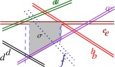
Figure 2.1: Vertical decomposition and the Clarkson-Shor framework. The defining set of ${{\sigma}}$ is ${{D}}\left({{{\sigma}}}\right)=\left\{{a,b,c,d}\right\}$, and its stopping set is ${{K}}\left({{{\sigma}}}\right)=\left\{{f}\right\}$.

Example 2.5.

Consider a set of segments ${{H}}$ in the plane. For a subset ${{R}}\subseteq{{H}}$, let ${{{{\mathop{\mathrm{\mathcal{A}}}}}^{|}}}\left({{{R}}}\right)$ denote the vertical decomposition of the plane formed by the arrangement ${{\mathop{\mathrm{\mathcal{A}}}}}({{R}})$ of the segments of ${{R}}$. This is the partition of the plane into interior disjoint vertical trapezoids formed by erecting vertical walls through each vertex of ${{\mathop{\mathrm{\mathcal{A}}}}}({{R}})$. Here, each object is a segment, a region is a vertical trapezoid, and ${{\mathcal{F}}}\left({{{R}}}\right)$ is the set of vertical trapezoids in ${{{{\mathop{\mathrm{\mathcal{A}}}}}^{|}}}\left({{{R}}}\right)$. Each trapezoid ${{\sigma}}\in{{\mathcal{F}}}\left({{{R}}}\right)$ is defined by at most four segments (or lines) of ${{R}}$ that define the region covered by the trapezoid ${{\sigma}}$, and this set of segments is ${{D}}\left({{{\sigma}}}\right)$. Here, ${{K}}\left({{{\sigma}}}\right)$ is the set of segments of ${{H}}$ intersecting the interior of the trapezoid ${{\sigma}}$ (see Figure 2.1).

Lemma 2.6.

Consider a canonical decomposition of a domain into simple cells, induced by a set of objects, that complies with the Clarkson-Shor framework [Cla88, CS89]. Then, performing a point location query in such a domain is equivalent to computing a basis of a violator space.

Proof:

This follows readily from definition, but we include the details for the sake of completeness. We use the notations of Definition 2.4 above.

So consider a fixed point ${{p}}\in{{\mathcal{D}}}$, and the task at hand is to compute the cell ${{\tau}}\in{{\mathcal{F}}}\left({{{H}}}\right)$ that contains ${{p}}$ (here, assuming general position implies that there is a unique such cell). In particular, for ${{R}}\subseteq{{H}}$, we define ${{B}}={{\mathrm{basis}}}\left({{{R}}}\right)$ to be the defining set of the cell ${{\tau}}$ of ${{\mathcal{F}}}\left({{{R}}}\right)$ that contains ${{p}}$, and the conflict list to be ${{\mathrm{cl}}}\left({{{R}}}\right)={{K}}\left({{{\tau}}}\right)$.

We claim that computing ${{\mathrm{basis}}}\left({{{H}}}\right)$ is a violator space problem. We need to verify the conditions of Definition 2.2, which is satisfyingly easy. Indeed, consistency is condition (i), and locality is condition (ii) in Definition 2.4. (We remind the reader that consistency and locality implies monotonicity, and thus we do not have to verify that it holds.) 

It seems that for all of these point location problems, one can solve them directly using the LP-type technique. However, stating these problems as violator space instances is more natural as it avoids the need to explicitly define an artificial ordering over the bases, which can be quite tedious and not immediate (see Appendix B for an example).

solveVS$\left({W,{{X}}\bigr{.}}\right)\Bigr{.}$: $\left\langle{{{f}}_{1},\ldots,{{f}}_{m}}\right\rangle$: A random permutation of the constraints of ${{X}}$. ${{B}}_{0}\leftarrow{{\color[rgb]{0.59,0,0.66}\texttt{\bf{comp{}Basis}}}}\left({W}\right)$ for $i=1$ to $m$ do if violate(${{f}}_{i},{{B}}_{i-1}$) then ${{B}}_{i}\leftarrow{{\color[rgb]{0.59,0,0.66}\texttt{\bf{solve{VS}}}}}\left({W\cup{{B}}_{i-1}\cup\left\{{{{f}}_{i}}\right\},\,\left\{{{{f}}_{1},\ldots,{{f}}_{i}}\right\}\bigr{.}}\right)$ else ${{B}}_{i}\leftarrow{{B}}_{i-1}$ return ${{B}}_{m}$

Figure 2.2: The algorithm for solving violator space problems. The parameter $W$ is a set of $O({{\delta}}^{2})$ witness constraints, and ${{X}}$ is a set of $m$ constraints. The function return ${{\mathrm{basis}}}\left({W\cup{{X}}}\right)$. To solve a given violator space, defined implicitly by the set of constraints ${{H}}$, and the functions violate and compBasis, one calls solveVS$\left({\left\{{}\right\},{{H}}}\right)$.

2.2 The algorithm for computing the basis of a violator space

The input is a violator space $\mathcal{V}=({{H}},{{\mathrm{cl}}})$ with $n=\left\lvert{{{H}}}\right\rvert$ constraints, having combinatorial dimension ${{\delta}}$.

2.2.1 Description of the algorithm

The algorithm is a variant of Seidel’s algorithm [Sei91] – it picks a random permutation of the constraints, and computes recursively in a randomized incremental fashion the basis of the solution for the first $i$ constraints. Specifically, if the $i$th constraint violates the basis ${{B}}_{i-1}$ computed for the first $i-1$ constraints, it calls recursively, adding the constraints of ${{B}}_{i-1}$ and the $i$th constraint to the set of constraints that must be included whenever computing a basis (in the recursive calls). The resulting code is depicted in Figure 2.2.

The only difference with the original algorithm of Seidel, is that the recursive call gets the set $W\cup{{B}}_{i-1}\cup\left\{{{{f}}_{i}}\right\}$ instead of ${{\mathrm{basis}}}\left({{{B}}_{i-1}\cup\left\{{{{f}}_{i}}\right\}}\right)$ (which is a smaller set). This modification is required because of the potential cycling between bases in a violator space.

2.2.2 Analysis

The key observation is that the depth of the recursion of solveVS is bounded by ${{\delta}}$, where ${{\delta}}$ is the combinatorial dimension of the violator space. Indeed, if ${{f}}_{i}$ violates a basis, the constraints added to the witness set $W$ guarantee that any subsequent basis computed in the recursive call contains ${{f}}_{i}$, as testified by the following lemma.

Lemma 2.7.

Consider any set ${{X}}\subseteq{{H}}$. Let ${{B}}={{\mathrm{basis}}}\left({{{X}}}\right)$, and let ${{f}}$ be a constraint in ${{H}}\setminus{{X}}$ that violates ${{B}}$. Then, for any subset ${{Y}}$ such that ${{B}}\cup\left\{{{{f}}}\right\}\subseteq{{Y}}\subseteq{{X}}\cup\left\{{{{f}}}\right\},$ we have that ${{f}}\in{{\mathrm{basis}}}\left({{{Y}}}\right)$.

Proof:

Assume that this is false, and let ${{Y}}$ be the bad set with ${{{B}^{\prime}}}={{\mathrm{basis}}}\left({{{Y}}}\right)$, such that ${{f}}\notin{{{B}^{\prime}}}$. Since ${{f}}\in{{Y}}$, by consistency, ${{f}}\notin{{\mathrm{cl}}}\left({{{Y}}}\right)$, see Definition 2.2. By definition ${{\mathrm{cl}}}\left({{{Y}}}\right)={{\mathrm{cl}}}\left({{{{B}^{\prime}}}}\right)$, which implies that ${{f}}\notin{{\mathrm{cl}}}\left({{{{B}^{\prime}}}}\right)$; that is, ${{f}}$ does not violate ${{{B}^{\prime}}}$.

Now, by monotonicity, we have ${{\mathrm{cl}}}\left({{{Y}}}\right)={{\mathrm{cl}}}\left({{{Y}}\setminus\left\{{{{f}}}\right\}}\right)={{\mathrm{cl}}}\left({{{{B}^{\prime}}}}\right).$

By assumption, ${{B}}\subseteq{{Y}}\setminus\left\{{{{f}}}\right\}$, which implies, again by monotonicity, as ${{B}}\subseteq{{Y}}\setminus\left\{{{{f}}}\right\}\subseteq{{X}}$, that ${{\mathrm{cl}}}\left({{{X}}}\right)={{\mathrm{cl}}}\left({{{Y}}\setminus\left\{{{{f}}}\right\}}\right)={{\mathrm{cl}}}\left({{{B}}}\right),$ as ${{B}}={{\mathrm{basis}}}\left({{{X}}}\right)$. But that implies that ${{\mathrm{cl}}}\left({{{B}}}\right)={{\mathrm{cl}}}\left({{{Y}}\setminus\left\{{{{f}}}\right\}}\right)={{\mathrm{cl}}}\left({{{{B}^{\prime}}}}\right).$ As ${{f}}\notin{{\mathrm{cl}}}\left({{{Y}}}\right)$, this implies that ${{f}}$ does not violate ${{B}}$, which is a contradiction.  

Lemma 2.8.

The depth of the recursion of solveVS, see Figure 2.2${}_{\text{p\ref{fig:V:S:algorithm}}}$, is at most ${{\delta}}$, where ${{\delta}}$ is the combinatorial dimension of the given instance.

Proof:

Consider a sequence of $k$ recursive calls, with $W_{0}\subseteq W_{1}\subseteq W_{2}\subseteq\cdots\subseteq W_{k}$ as the different values of the parameter $W$ of solveVS, where $W_{0}=\emptyset$ is the value in the top-level call. Let ${{g}}_{j}$, for $j=1,\ldots,k$, be the constraint whose violation triggered the $j$th level call. Observe that ${{g}}_{j}\in W_{j}$, and as such all these constraints must be distinct (by consistency). Furthermore, we also included the basis ${{B}}_{j}^{\prime}$, that ${{g}}_{j}$ violates, in the witness set $W_{j}$. As such, we have that $W_{j}=\left\{{{{g}}_{1},\ldots,{{g}}_{j}}\right\}\cup{{B}}_{1}^{\prime}\cup\cdots\cup{{B}}_{j}^{\prime}.$ By Lemma 2.7, in any basis computation done inside the recursive call ${{\color[rgb]{0.59,0,0.66}\texttt{\bf{solve{VS}}}}}\left({W_{j},\ldots}\right)$, it must be that ${{g}}_{j}\in{{\mathrm{basis}}}\left({W_{t}}\right)$, for any $t\geq j$. As such, we have ${{g}}_{1},\ldots,{{g}}_{k}\in{{\mathrm{basis}}}\left({W_{k}}\right)$. Since a basis can have at most ${{\delta}}$ elements, this is possible only if $k\leq{{\delta}}$, as claimed.  

Theorem 2.9.

Given an instance of violator space $\mathcal{V}=({{H}},{{\mathrm{cl}}})$ with $n$ constraints, and combinatorial dimension ${{\delta}}$, the algorithm solveVS$\left({\emptyset,{{H}}}\right)$, see Figure 2.2, computes ${{\mathrm{basis}}}\left({{{H}}}\right)$. The expected number of violation tests performed is bounded by $O({{\delta}}^{{{\delta}}+1}n)$. Furthermore, the algorithm performs in expectation $O\left({\left({{{\delta}}\ln n}\right)^{{\delta}}}\right)$ basis computations (on sets of constraints that contain at most ${{\delta}}({{\delta}}+1)$ constraints).

In particular, for constant combinatorial dimension ${{\delta}}$, with violation test and basis computation that takes constant time, this algorithm runs in $O(n)$ expected time.

Proof:

Lemma 2.8 implies that the recursion tree has bounded depth, and as such this algorithm must terminate. The correctness of the result follows by induction on the depth of the recursion. By Lemma 2.8, any call of depth ${{\delta}}$, cannot find any violated constraint in its subproblem, which means that the returned basis is indeed the basis of the constraints specified in its subproblem. Now, consider a recursive call at depth $j<{{\delta}}$, which returns a basis ${{B}}_{m}$ when called on the constraints $\left\langle{{{f}}_{1},\ldots,{{f}}_{m}}\right\rangle$. The basis ${{B}}_{m}$ was computed by a recursive call on some prefix $\left\langle{{{f}}_{1},\ldots,{{f}}_{i}}\right\rangle$, which was correct by (reverse) induction on the depth, and none of the constraints ${{f}}_{i+1},\ldots,{{f}}_{m}$ violates ${{B}}_{m}$, which implies that the returned basis is a basis for the given subproblem. Thus, the result returned by the algorithm is correct.

Let $C_{k}(m)$ be the expected number of basis computations performed by the algorithm when run at recursion depth $k$, with $m$ constraints. We have that $C_{{{\delta}}}(m)=1$, and $C_{k}(m)=1+\mathop{\mathbf{E}}\left[{\Bigl{.}\sum_{i=1}^{m}X_{i}C_{k+1}(i)}\right],$ where $X_{i}$ is an indicator variable that is one, if and only if the insertion of the $i$th constraint caused a recursive call. We have, by backward analysis, that $\mathop{\mathbf{E}}\left[{X_{i}}\right]=\mathop{\mathbf{Pr}}\left[{X_{i}=1}\right]\leq\min\left({{{{\delta}}}/{i},1}\right).$ As such, by linearity of expectations, we have $C_{k}(m)\leq 1+\sum_{i=1}^{m}\min\left({\frac{{{\delta}}}{i},1}\right)C_{k+1}(i).$ As such, we have

$$C_{{{\delta}}-1}(m)\leq 1+\sum_{i=1}^{m}\min\left({\frac{{{\delta}}}{i},1}\right)C_{{{\delta}}}(i)={{\delta}}+\sum_{i={{\delta}}}^{m}\frac{{{\delta}}}{i}\leq{{\delta}}+{{\delta}}\ln(m/{{\delta}})\leq{{\delta}}\ln(m),$$

assuming ${{\delta}}\geq e$. We conclude that $C_{{{\delta}}-1}(m)\leq{{\delta}}\ln(m)$ and $C_{0}(m)=O\left({\left({{{\delta}}\ln m}\right)^{{\delta}}}\right)$.

As for the expected number of violation tests, a similar analysis shows that $V_{{\delta}}(m)=m$ and $V_{{{\delta}}-j}(m)=m+\sum_{i=1}^{m}\min\left({\frac{{{\delta}}}{i},1}\right)V_{{{\delta}}-(j-1)}(i).$ As such, assuming inductively that $V_{{{\delta}}-(j-1)}(m)\leq j{{\delta}}^{j-1}m$, we have that

$$V_{{{\delta}}-j}(m) \leq m+\sum_{i=1}^{m}\frac{{{\delta}}}{i}j{{\delta}}^{j-1}i\leq m+j{{\delta}}^{j}m\leq(j+1){{\delta}}^{j}m,$$

implying that $V_{0}(m)=O({{\delta}}^{{{\delta}}+1}m)$, which also bounds the running time.  

Remark 2.10.

While the constants in Theorem 2.9 are not pretty, we emphasize that the $O$ notation in the bounds do not hide constants that depends on ${{\delta}}$.

2.3 Solving the violator space problem with constant space and linear time

The idea for turning solveVS into an algorithm that uses little space, is observing that the only thing we need to store (implicitly) is the random permutation used by solveVS.

2.3.1 Generating a random permutation using pseudo-random generators

To avoid storing the permutation, one can use pseudo-random techniques to compute the permutation on the fly. For our algorithm, we do not need a permutation - any random sequence that has uniform distribution over the constraints and is sufficiently long, would work.

Lemma 2.11.

Fix an integer ${{\phi}}>0$, a prime integer $n$, and an integer constant $c^{\prime}\geq 12$. One can compute a random sequence of numbers $X_{1},\ldots,X_{c^{\prime}n}\in\left\llbracket n\right\rrbracket=\left\{{1,\ldots,n}\right\}$, such that:

1. The probability of $X_{i}=j$ is $1/n$, for any $i\in\left\llbracket n\right\rrbracket$ and $j\in\left\llbracket c^{\prime}n\right\rrbracket$.

2. The sequence is ${{\phi}}$-wise independent.

3. Using $O(c^{\prime}{{\phi}})$ space, given an index $i$, one can compute $X_{i}$ in $O({{\phi}})$ time.

Proof:

This is a standard pseudo-random generator (PRG) technique, described in detail by Mulmuley [Mul94, p. 399]. We outline the idea. Randomly pick ${{\phi}}+1$ coefficients $\alpha_{0},\ldots,\alpha_{{{\phi}}}\in\left\{{0,\ldots,n-1}\right\}$ (uniformly and independently), and consider the random polynomial $f(x)=\sum_{i=0}^{{{\phi}}}\alpha_{i}x^{i}$, and set $p(x)=(f(x)\mod n)$. Now, set $X_{i}=1+p(i)$, for $i=1,\ldots,n$. It is easy to verify that the desired properties hold. To extent this sequence to be of the desired length, pick randomly $c^{\prime}$ such polynomials, and append their sequences together to get the desired longer sequence. It is easy to verify that the longer sequence is still ${{\phi}}$-wise independent.  

We need the following concentration result on $2k$-wise independent sequences – for the sake completeness, we provide a proof at Appendix A.1.

Lemma 2.12 (Theorem A.2.1, [Mul94]).

Let $X_{1},\ldots,X_{n}$ be $n$ random indicator variables that are $2{{\psi}}$-wise independent, where $p=\mathop{\mathbf{Pr}}\left[{X_{i}=1}\right]\geq 1/n$, for all $i$. Let $\Bigl{.}Y=\sum_{i}X_{i}$, and let $\mu=\mathop{\mathbf{E}}\left[{Y}\right]=pn$. Then, we have that $\mathop{\mathbf{Pr}}\left[{\bigl{.}Y=0}\right]\leq\mathop{\mathbf{Pr}}\left[{\bigl{.}\left\lvert{Y-\mu}\right\rvert\geq\mu}\right]\leq\left({4{{\psi}}^{2}/\mu\bigr{.}}\right)^{{\psi}}/\sqrt{2{{\psi}}}.$

The following lemma testifies that this PRG sequence, with good probability, contains the desired basis (as such, conceptually, we can think about it as being a permutation of $\left\llbracket n\right\rrbracket$).

Lemma 2.13.

Let ${{B}}\subseteq\left\llbracket n\right\rrbracket$ be a specific set of ${{\delta}}$ numbers. Fix an integer ${{\phi}}\geq 8+2{{\delta}}$, and let ${{\mathcal{X}}}=\left\langle{X_{1},\ldots,X_{c^{\prime}n}}\right\rangle$ be a ${{\phi}}$-wise independent random sequence of numbers, each uniformly distributed in $\left\llbracket n\right\rrbracket$, where $c^{\prime}$ is any constant $\geq{{8\left({5+\left\lceil{\ln\delta}\right\rceil}\right)^{2}}}$. Then, the probability that the elements of ${{B}}$ do not appear in ${{\mathcal{X}}}$ is bounded by, say, $1/20$.

Proof:

Fix an element $b$ of ${{B}}$. Let $Y_{i}$ be an indicator variable that is one $\iff$ $X_{i}=b$. Observe that $p=\mathop{\mathbf{Pr}}\left[{Y_{i}=1}\right]=1/n$. As such, we have that $\mu=\mathop{\mathbf{E}}\left[{\sum_{i=1}^{c^{\prime}n}Y_{i}}\right]=c^{\prime}=8k^{2},$ for $k=5+\left\lceil{\ln{{\delta}}}\right\rceil$.

As $k\leq{{\phi}}/2$, we can interpret ${{\mathcal{X}}}$ as a $2k$-wise independent sequence. By Lemma 2.12, we have that the probability that $b$ does not appear in ${{\mathcal{X}}}$ is bounded by $\mathop{\mathbf{Pr}}\left[{\sum_{i}Y_{i}=0}\right]\leq\left({4k^{2}/\mu}\right)^{k}/\sqrt{2k}.$ We want this probability to be smaller than $1/(20{{\delta}})$, Since $\mu=8k^{2}$, this is equivalent to $\left({4k^{2}/\mu}\right)^{k}{{\delta}}\leq{\sqrt{2k}}/{20}\iff{{\delta}}\leq 2^{k}{\sqrt{2k}}/{20}$ which holds as $2^{k}\geq 32{{\delta}}$.

Now, by the union bound, the probability that any element of ${{B}}$ does not appear in ${{\mathcal{X}}}$ is bounded by ${{{\delta}}}/(20{{{\delta}}})={1}/{20}$.  

Remark 2.14.

There are several low level technicalities that one needs to address in using such a PRG sequence instead of a truly random permutation:

1. Repeated numbers are not a problem: the algorithm solveVS (see Figure 2.2${}_{\text{p\ref{fig:V:S:algorithm}}}$) ignores a constraint that is being inserted for the second time, since it cannot violate the current basis.

2. Verifying the solution: The sequence (of the indices) of the constraints used by the algorithm would be $X_{1},\ldots,X_{c^{\prime}n}$. This sequence might miss some constraints that violate the computed solution.

   As such, in a second stage, the algorithm checks if any of the constraints $1,2,\ldots,n$ violates the basis computed. If a violation was found, then the sequence generated failed, and the algorithm restarts from scratch – resetting the PRG used in this level, regenerating the random keys used to initialize it, and rerun it to generate a new sequence. Lemma 2.13 testifies that the probability for such a failure is at most $1/20$ – thus restarting is going to be rare.

3. Independence between levels: We will use a different PRG for each level of the recursion of solveVS. Specifically, we generate the keys used in the PRG in the beginning of each recursive call. Since the depth of the recursion is ${{\delta}}$, that increases the space requirement by a factor of ${{\delta}}$.

4. If the subproblem size is not a prime: In a recursive call, the number of constraints given (i.e., $m$) might not be a prime. To this end, the algorithm can store (non-uniformly), a list of primes, such that for any $m$, there is a prime $m^{\prime}\geq m$ that is at most twice bigger than $m$. Then the algorithm generates the sequence modulo $m^{\prime}$, and ignores numbers that are larger than $m$. This implies that the sequence might contain invalid numbers, but such numbers are only a constant fraction of the sequence, so ignoring them does not change the running time analysis of our algorithm. (More precisely, this might cause the running time of the algorithm to deteriorate by a factor of $\exp(O({{\delta}}))$, but as we consider ${{\delta}}$ to be a constant, this does not effect our analysis.)

One needs now to prove that backward analysis still works for our algorithm for violator spaces. The proof of the following lemma is implied by a careful tweaking of Mulmuley’s analysis – we provide the details in Appendix A.

Lemma 2.15 (See Appendix A).

Consider a violator space $\mathcal{V}=({{H}},{{\mathrm{cl}}})$ with $n=\left\lvert{{{H}}}\right\rvert$, and combinatorial dimension ${{\delta}}$. Let ${{\mathcal{X}}}=X_{1},X_{2},\ldots,$ be a random sequence of constraints of ${{H}}$ generated by a ${{\phi}}$-wise independent distribution (with each $X_{i}$ having a uniform distribution), where ${{\phi}}>6{{\delta}}+9$ is a constant. Then, for $i>2{{\delta}}$, the probability that $X_{i}$ violates ${{B}}={{\mathrm{basis}}}\left({X_{1},\ldots,X_{i-1}}\right)$ is $O(1/i)$.

Remark.

Lemma 2.15 states that backwards analysis works on pseudo-random sequences when applied to the Clarkson-Shor [Cla88, CS89] settings, where the defining set of the event (or basis) of interest has constant size. However, there are cases when one would like to apply backwards analysis when the defining set might have an unbounded size, and the above does not hold in this case.

For an example where a defining set might have unbounded size, consider a random permutation of points, and the event being a point being a vertex of the convex-hull of the points inserted so far. This is used in a recent proof showing that the complexity of the convex-hull of $n$ points, picked uniformly and randomly, in the hypercube in $d$ dimensions has $O(\log^{d-1}n)$ vertices, with high probability [CHR15],

2.3.2 The result

Theorem 2.16.

Given an instance of a violator space $\mathcal{V}=({{H}},{{\mathrm{cl}}})$ with $n$ constraints, and combinatorial dimension ${{\delta}}$, one can compute ${{\mathrm{basis}}}\left({{{H}}}\right)$ using $O\left({{{\delta}}^{2}\log^{2}{{\delta}}}\right)$ space. For some constant ${{\zeta}}=O\left({{{\delta}}\log^{2}{{\delta}}}\right)$, we have that:

1. The expected number of basis computations is $O\left({\bigl{.}\smash{\left({{{\zeta}}\ln n}\right)^{{\delta}}}}\right)$, each done over $O({{\delta}}^{2})$ constraints.

2. The expected number of violation tests performed is $O\bigl{(}{{\zeta}}^{{\delta}}n\bigr{)}$.

3. The expected running time (ignoring the time to do the above operations) is $O\bigl{(}{{\zeta}}^{{\delta}}n\bigr{)}$.

Proof:

The algorithm is described above. As for the analysis, it follows by plugging the bound of Lemma 2.15 into the proof of Theorem 2.9.

The only non-trivial technicality is to handle the case that the PRG sequence fails to contain the basis. Formally, abusing notations somewhat, consider a recursive call on the constraints indexed by $\left\llbracket n\right\rrbracket$, and let ${{B}}$ be the desired basis of the given subproblem. By Lemma 2.13, the probability that ${{B}}$ is not contained in the generated PRG is bounded by $1/20$ – and in such a case the sequence has to be regenerated till success. As such, in expectation, this has a penalty factor of (say) $2$ on the running time in each level. Overall, the analysis holds with the constants deteriorating by a factor of (at most) $2^{{\delta}}$.  

Remark 2.17.

Note, that the above pseudo-random generator technique is well known, but using it for linear programming by itself does not make too much sense. Indeed, pseudo-random generators are sometimes used as a way to reduce the randomness consumed by an algorithm. That in turn is used to derandomize the algorithm. However, for linear programming Megiddo’s original algorithm was already linear time deterministic. Furthermore, Chazelle and Matoušek [CM96], using different techniques showed that one can even derandomize Clarkson’s algorithm and get a linear running time with a better constant.

Similarly, using PRGs to reduce space of algorithms is by now a standard technique in streaming, see for example the work by Indyk [Ind06], and references therein.

3 Corridor decomposition

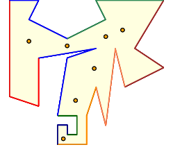
(i)	(ii)	(iii)

Figure 3.1: An example of a corridor decomposition for a polygon: (i) Input curves, medial axis and active vertices, (ii) their critical circles, and their spokes, and (iii) the resulting corridor decomposition.

3.1 Construction

The decomposition here is similar to the decomposition described by the author in a recent work [Har14].

Definition 3.1 (Breaking a polygon into curves).

Let the given polygon ${{P}}$ have the vertices $v_{1},\ldots v_{n}$ in counterclockwise order along its boundary. Let $\sigma_{i}$ be the polygonal curve having the vertices $v_{(i-1){{m}}+1},v_{(i-1){{m}}+2},\linebreak[1]v_{(i-1){{m}}+3},\ldots,v_{i{{m}}+1},$ for $i=1,\ldots,{{\overline{{n}}}}-1$, where

$${{\overline{{n}}}}=\left\lfloor{(n-1)/{{m}}}\right\rfloor+1.$$

The last polygonal curve is $\sigma_{{{\overline{{n}}}}}=v_{({{\overline{{n}}}}-1){{m}}+1},v_{({{\overline{{n}}}}-1){{m}}+2},\ldots v_{n},v_{1}$. Note, that given ${{P}}$ in a read only memory, one can encode any curve $\sigma_{i}$ using $O(1)$ space. Let $\Gamma=\left\{{\sigma_{1},\ldots,\sigma_{{{\overline{{n}}}}}}\right\}$ be the resulting set of polygonal curves. From this point on, a curve refers to a polygonal curve generated by this process.

3.1.1 Corridor decomposition for the whole polygon

Next, consider the medial axis of ${{P}}$ restricted to the interior of ${{P}}$ (see Chin et al. [CSW99] for the definition and an algorithm for computing the medial axis of a polygon). A vertex $v$ of the medial axis corresponds to a disk $D$, that touches the boundary of ${{P}}$ in two or three points (by the general position assumption, that the medial axis of the polygon does not have degenerate vertices, not in any larger number of points). The medial axis has the topological structure of a tree.

To make things somewhat cleaner, we pretend that there is a little hole centered at every vertex of the polygon if it is the common endpoint of two curves. This results in a medial axis edge that comes out of the vertex as an angle bisector, both for an acute angle (where a medial axis edge already exists), and for obtuse angles, see Figure 3.1 and Figure 3.3.

A vertex of the medial axis is active if its disk touches three different curves of $\Gamma$. It is easy to verify that there are $O({{\overline{{n}}}})$ active vertices. The segments connecting an active vertex to the three (or two) points of tangency of its empty disk with the boundary of ${{P}}$ are its spokes or doors. Introducing these spokes breaks the polygon into the desired corridors.

Such a corridor is depicted on the right. It has a floor and a ceiling – each is a subcurve of some input curve. In addition, each corridor might have four additional doors grouped into “double” doors. Such a double door is defined by an active vertex and two segments emanating from it to the floor and ceiling curves, respectively. We refer to such a double door as an gate. As such, specifying a single corridor requires encoding the vertices of the two gates and the floor and ceiling curves, which can be done in $O(1)$ space, given the two original curves. In particular, a corridor is defined by four curves – a ceiling curve, floor curve, and two additional curves inducing the two gates.

Here is an informal argument why corridors indeed have the above described structure. If there is any other curve, except the floor and the ceiling, that interacts with the interior of the corridor, then this curve would break the corridor into smaller sub-corridors, as there would be a medial axis vertex corresponding to three curves in the interior of the corridor, which is impossible.

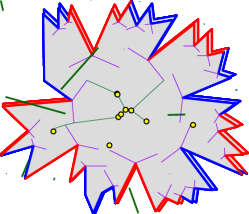
(i)	(ii)	(iii)

Figure 3.3: Another example of a corridor decomposition for a polygon: (i) Input polygon and its curves and its medial axis (the thick lines are the angle bisectors for the obtuse angles where two curves meet), (ii) active vertices and their spokes (with a reduced medial axis), and (iii) the resulting corridor decomposition.

(i)	(ii)	(iii)

Figure 3.4: Corridor decomposition for disjoint curves: (i) Input curves, the medial axis, and active vertices, (ii) the critical circles, and their spokes, and (iii) the resulting corridor decomposition.

3.1.2 Corridor decomposition for a subset of the curves

For a subset $\Psi\subseteq\Gamma$, of total complexity ${\mathsf{t}}$, one can apply a similar construction. Again, compute the medial axis of the curves of $\Psi$, by computing, in $O({\mathsf{t}}\log{\mathsf{t}})$ time, the Voronoi diagram of the segments used by the curves [For87], and extracting the medial axis (it is now a planar graph instead of a tree). Now, introducing the spokes of the active vertices, results in a decomposition into corridors. For technical reasons, it is convenient to add a large bounding box, and restrict the construction to this domain, treating this frame as yet another input curve. Figure 3.4 depicts one such corridor decomposition.

Let $\mathcal{C}\left({\Psi}\right)$ denote this resulting decomposition into corridors.

3.1.3 Properties of the resulting decomposition

Every corridor in the resulting decomposition $\mathcal{C}\left({\Psi}\right)$ is defined by a constant number of input curves. Specifically, consider the set of all possible corridors; that is $\mathcal{F}=\bigcup_{\Upsilon\subseteq\Gamma}\mathcal{C}\left({\Upsilon}\right).$ Next, consider any corridor ${{C}}\in\mathcal{F}$, then there is a unique defining set ${{D}}\left({{{C}}}\right)\subseteq\Psi$ (of at most $4$ curves). Similarly, such a corridor has stopping set (or conflict list) of ${{C}}$, denoted by ${{K}}\left({{{C}}}\right)$. Here, the defining set of a corridor, as depicted by Figure 3.2, is formed by the floor and the ceiling curves of the corridor, and the two external curves defining the two gates. The stopping set contains all the curves that intersect the interior of the corridor, or the interior of the two disks that define the two gates.

Consider any subset $\mathcal{S}\subseteq\Gamma$. It is easy to verify that the following two conditions hold:

1. For any $C\in\mathcal{C}\left({\mathcal{S}}\right)$, we have ${{D}}\left({C}\right)\subseteq\mathcal{S}$ and $\mathcal{S}\cap{{K}}\left({C}\right)=\emptyset$.

2. If ${{D}}\left({C}\right)\subseteq\mathcal{S}$ and ${{K}}\left({C}\right)\cap\mathcal{S}=\emptyset$, then $C\in\mathcal{C}\left({\mathcal{S}}\right)$.

Namely, the corridor decomposition complies with the technique of Clarkson-Shor (see Section 2.1.2 and Definition 2.4).

3.2 Computing a specific corridor

Let ${{p}}$ be a point in the plane, and let $\Gamma$ be a set of ${{\overline{{n}}}}$ interior disjoint curves (stored in a read only memory), where each curve is of complexity ${{m}}$. Let $n$ be the total complexity of these curves (we assume that $n=\Theta({{m}}\,{{\overline{{n}}}})$). Our purpose here is to compute the corridor ${{C}}\in\mathcal{C}\left({\Gamma}\right)$ that contains ${{p}}$. Formally, for a subset $\Psi\subseteq\Gamma$, we define the function $w(\Psi)$, to be the defining set of the corridor ${{C}}\in\mathcal{C}\left({\Psi}\right)$ that contains ${{p}}$. Note, that such a defining set has cardinality at most ${{\delta}}=4$.

3.2.1 Basic operations

We need to specify how to implement the two basic operations:

1. (Basis computation) Given a set of $O(1)$ curves, we compute their medial axis, and extract the corridor containing ${{p}}$. This takes $O({{m}}\log{{m}})$ time, and uses $O({{m}})$ work space.

2. (Violation test) Given a corridor ${{C}}$, and a curve $\sigma$, both of complexity $O({{m}})$, we can check if $\sigma$ violates the corridor by checking if an arbitrary vertex of $\sigma$ is contained in ${{C}}$ (this takes $O({{m}})$ time to check), and then check in $O({{m}})$ time, if any segment of $\sigma$ intersects the two gates of ${{C}}$. More precisely, each gate has an associated empty disk with it. The corridor is violated if the curve $\sigma$ intersect these two empty disks associated with the two gates of the corridor, see Figure 3.2. Overall, this takes $O({{m}})$ time.

We thus got the following result.

Lemma 3.2.

Given a polygon ${{P}}$ with $n$ vertices, stored in read only memory, and let ${{m}}$ be a parameter. Let $\Gamma$ be the set of ${{\overline{{n}}}}$ curves resulting from breaking ${{P}}$ into polygonal curves each with ${{m}}$ vertices, as described in Definition 3.1. Then, given a query point ${{p}}$ inside ${{P}}$, one can compute, in $O(n+{{m}}\log{{m}}\log^{4}(n/{{m}}))$ expected time, the corridor of $\mathcal{C}\left({\Gamma}\right)$ that contains ${{p}}$. This algorithm uses $O({{m}})$ work space.

Proof:

As described above, this problem is a point location problem in a canonical decomposition; that is, a violator space problem. Plugging it into Theorem 2.16, makes in expectation $O({{\overline{{n}}}})$ violation tests, each one takes $O({{m}})$ time, where ${{\overline{{n}}}}=\left\lfloor{(n-1)/{{m}}}\right\rfloor+1=O(n/{{m}})$. The algorithm performs in expectation $O(\log^{4}{{\overline{{n}}}})$ basis computations, each one takes $O({{m}}\log{{m}})$ time. Thus, expected running time is $O({{\overline{{n}}}}\cdot{{m}}+{{m}}\log{{m}}\log^{4}{{\overline{{n}}}})$ time. As for the space required, observe that a corridor can be described using $O(1)$ space.

The algorithm needs $O({{m}})$ work space to implement the basis computation operation, as all other portions of the algorithm require only constant additional work space.  

We comment that the problem of Lemma 3.2 can also be solved as an LP-type problem. We refer the interested reader to Appendix B.

4 Shortest path in a polygon in sublinear space

Let ${{P}}$ be a simple polygon with $n$ edges in the plane, and let ${{s}}$ and ${{t}}$ be two points in ${{P}}$, where $s$ is the source, and $t$ is the target. Our purpose here is to compute the shortest path between $s$ and $t$ inside ${{P}}$. The vertices of ${{P}}$ are stored in (say) counterclockwise order in an array stored in a read only memory. Let ${{m}}$ be a prespecified parameter that is (roughly) the amount of additional space available for the algorithm.

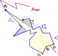
(i) (ii) (iii)

Figure 4.1: (i) The state in the beginning of the $i$th iteration. (ii) The clipped polygon ${{C}}_{i}^{\prime}$. (iii) The funnel created by the shortest paths from ${{s}}_{i}$ to the two spoke endpoints.

4.1 Updating the shortest path through a corridor

We remind the reader that a corridor has two double doors, see Figure 3.2${}_{\text{p\ref{fig:doors}}}$. The rest of the boundary of the corridor is made out two chains from the original polygon.

Given two rays $\sigma$ and $\sigma^{\prime}$, that share their source vertex $v$ (which lies inside ${{P}}$), consider the polygon ${{Q}}$ that starts at $v$, follows the ray $\sigma$ till it hits the boundary of ${{P}}$, then trace the boundary of ${{P}}$ in a counterclockwise direction till the first intersection of $\sigma^{\prime}$ with $\partial{{P}}$, and then back to $v$. The polygon ${{Q}}={{P}}\!\left\langle{\sigma,\sigma^{\prime}}\right\rangle$ is the clipped polygon. See Figure 4.1 (ii).

A geodesic is the shortest path between two points (restricted to lie inside ${{P}}$). Two geodesics might have a common intersection, but they can cross at most once. Locally, inside a polygon, a geodesic is a straight segment. For our algorithm, we need the following two basic operations (both can be implemented using $O(1)$ work space):

1. isPntIn(${{p}}$): Given a query point ${{p}}$, it decides if ${{p}}$ is inside ${{P}}$. This is done by scanning the edges of ${{P}}$ one by one, and counting how many edges cross the vertical ray shooting from ${{p}}$ downward. This operation takes linear time (in the number of vertices of ${{P}}$). If the count is odd then ${{p}}$ is inside ${{P}}$, and it is outside otherwise.

2. isInSubPoly(${{p}},\sigma,\sigma^{\prime}$): returns true if ${{p}}$ is in the clipped polygon ${{P}}\!\left\langle{\sigma,\sigma^{\prime}}\right\rangle$. This can be implemented to work in linear time and constant space, by straightforward modification of isPntIn.

Using vertical and horizontal rays shot from ${{s}}$, one can decide, in $O(n)$ time, which quadrant around ${{s}}$ is locally used by the shortest path from ${{s}}$ to ${{t}}$. Assume that this path is in the positive quadrant. It would be useful to think about geodesics starting at ${{s}}$ as being sorted angularly. Specifically, if $\tau$ and $\tau^{\prime}$ are two geodesic starting at ${{s}}$, then $\tau$ is to the left of $\tau^{\prime}$, if the first edge of $\tau$ is counterclockwise to the first edge of $\tau^{\prime}$. If the prefix of $\tau$ and $\tau^{\prime}$ is non-empty, we apply the same test to the last common point of the two paths. Let $\tau\prec\tau^{\prime}$ denote that $\tau$ is to the left of $\tau^{\prime}$.

In particular, if the endpoint of the rays $\sigma,\sigma^{\prime}$ is the source vertex ${{s}}$, and the geodesic between ${{s}}$ and ${{t}}$ lies in ${{P}}\!\left\langle{\sigma,\sigma^{\prime}}\right\rangle$, then given a third ray $\pi$ lying between $\sigma$ and $\sigma^{\prime}$, the shortest path between ${{s}}$ and ${{t}}$ in ${{P}}$ must lie completely either in ${{P}}\!\left\langle{\sigma,\pi}\right\rangle$ or ${{P}}\!\left\langle{\pi,\sigma^{\prime}}\right\rangle$, and this can be tested by a single call to isInSubPoly for checking if ${{t}}$ is in ${{P}}\!\left\langle{\pi,\sigma^{\prime}}\right\rangle$.

4.1.1 Limiting the search space

Lemma 4.1.

Let ${{P}}$, ${{s}}$ and ${{t}}$ be as above, and $\mu$ be the shortest path from ${{s}}$ to ${{t}}$ in ${{P}}$. Let ${{p}}{{q}}$ be a given edge, which is the last edge in the shortest path $\tau$ from ${{s}}$ to ${{q}}$, where ${{q}}$ is in ${{P}}$. Then, one can decide in $O(n)$ time, and using $O(1)$ space, if $\mu\prec\tau$, where $n$ is the number of vertices of ${{{P}}}$.

Proof:

If ${{p}}={{s}}$, then this can be determined by shooting two rays, one in the direction of ${{s}}\rightarrow{{q}}$ and the other in the opposite direction, where ${{s}}\rightarrow{{q}}$ denotes the vector ${{q}}-{{s}}$. Then a single call to isInSubPoly resolves the issue.

Otherwise, ${{p}}$ must be a vertex of ${{P}}$. Consider the ray $\sigma$ starting at ${{p}}$ (or ${{q}}$ – that does not matter) in the direction of ${{p}}\rightarrow{{q}}$. Compute, in linear time, the first intersection of this ray with the boundary of ${{P}}$, and let ${{u}}$ be this point. Clearly, ${{p}}{{u}}$ connects two points on the boundary of ${{P}}$, and it splits ${{P}}$ into two polygons. One can now determine, in linear time, which of these two polygons contains ${{t}}$, thus resolving the issue.  

4.1.2 Walking through a corridor

In the beginning of the $i$th iteration of the algorithm it would maintains the following quantities (depicted in Figure 4.1 (i)):

1. ${{s}}_{i}$: the current source (it lies on the shortest path $\mu_{\mathrm{opt}}$ between ${{s}}$ and ${{t}}$).

2. ${{C}}_{i}$: The current corridor.

3. $\triangle_{i}$: A triangle having ${{s}}_{i}$ as one of its vertices, and its two other vertices lie on a spoke of ${{C}}_{i}$. The shortest path $\mu_{\mathrm{opt}}$ passes through ${{s}}_{i}$, and enters ${{C}}_{i}$ through the base of $\triangle_{i}$, and then exits the corridor through one of its “exit” spokes.

The task at hand is to trace the shortest path through ${{C}}_{i}$, in order to compute where the shortest path leaves the corridor.

Lemma 4.2.

Tracing the shortest path $\mu_{\mathrm{opt}}$ through a single corridor takes $O\bigl{(}n\log{{m}}+{{m}}\log{{m}}\log^{4}{{\overline{{n}}}}\bigr{)}$ expected time, using $O({{m}})$ space.

Proof:

We use the above notation. The algorithm glues together $\triangle_{i}$ to ${{C}}_{i}$ to get a new polygon. Next, it clips the new polygon by extending the two edges of $\triangle_{i}$ from ${{s}}_{i}$. Let ${{C}}_{i}^{\prime}$ denote the resulting polygon, depicted in Figure 4.1 (ii). Let the three vertices of ${{C}}_{i}^{\prime}$ forming the two “exit” spokes be ${{p}}_{i},{{q}}_{i},{{u}}_{i}$. Next, the algorithm computes the shortest path from ${{s}}_{i}$ to the three vertices ${{p}}_{i},{{q}}_{i},{{u}}_{i}$ inside ${{C}}_{i}^{\prime}$, and let $\pi_{i},\pi_{i}^{\prime},\pi_{i}^{\prime\prime}$ be these paths, respectively (this takes $O(\left\lvert{{{C}}_{i}^{\prime}}\right\rvert)=O({{m}})$ time [GH89] after linear time triangulation of the polygon [Cha91, AGR01]). Using Lemma 4.1 the algorithm decides if $\pi_{i}\prec\mu_{\mathrm{opt}}\prec\pi_{i}^{\prime}$ or $\pi_{i}^{\prime}\prec\mu_{\mathrm{opt}}\prec\pi_{i}^{\prime\prime}$. We refer to a prefix path (that is part of the desired shortest path) followed by the two concave chains as a funnel – see Figure 4.1 (iii) and Figure 4.2 for an example.

Assume that $\pi_{i}\prec\mu_{\mathrm{opt}}\prec\pi_{i}^{\prime}$, and let $F_{i}$ be the funnel created by these two shortest paths, where ${{p}}_{i}{{q}}_{i}$ is the base of the funnel. If the space bounded by the funnel is a triangle, then the algorithm sets its top vertex as ${{s}}_{i+1}$, the funnel triangle is $\triangle_{i+1}$, and the algorithm computes the corridor on the other side of ${{p}}_{i}{{q}}_{i}$ using the algorithm of Lemma 3.2 (by picking any point on ${{p}}_{i}{{q}}_{i}$ as the query for the point location operation), set it as ${{C}}_{i+1}$, and continues the execution of the algorithm to the next iteration.

The challenge is handling funnel chains that are “complicated” concave polygons (with at most $O({{m}})$ vertices), see Figure 4.2. As long as the funnel $F_{i}$ is not a triangle, pick a middle edge $e$ on one side of the funnel, and extend it till it hits the edge ${{p}}_{i}{{p}}_{i+1}$, at a point ${{x}}$. This breaks $F_{i}$ into two funnels, and using the algorithm of Lemma 4.1 on the edge $e$, decide which of these two funnels contains the shortest path $\mu_{\mathrm{opt}}$, and replace $F_{i}$ by this funnel. Repeat this process till $F_{i}$ becomes a triangle. Once this happens, the algorithm continues to the next iteration as described above. Clearly, this funnel “reduction” requires $O(\log{{m}})$ calls to the algorithm of Lemma 4.1.

Note, that the algorithm “forgets” the portion of the funnel that is common to both paths as it moves from ${{C}}_{i}$ to ${{C}}_{i+1}$. This polygonal path is a part of the shortest path $\mu_{\mathrm{opt}}$ computed by the algorithm, and it can be output at this stage, before moving to the next corridor ${{C}}_{i+1}$.

Figure 4.2:
Funnel reduction.

In the end of the iteration, this algorithm computes the next corridor ${{C}}_{i+1}$ by calling the algorithm of Lemma 3.2.  

4.2 The algorithm

The overall algorithm works by first computing the corridor ${{C}}_{1}$ containing the source ${{s}}_{1}={{s}}$ using Lemma 3.2. The algorithm now iteratively applies Lemma 4.2 till arriving to the corridor containing ${{t}}$, where the remaining shortest path can be readily computed. Since every corridor gets visited only once by this walk, we get the following result.

Theorem 4.3.

Given a simple polygon ${{P}}$ with $n$ vertices (stored in a read only memory), a start vertex ${{s}}$, a target vertex ${{t}}$, and a space parameter ${{m}}$, one can compute the length of the shortest path from ${{s}}$ to ${{t}}$ (and output it), using $O({{m}})$ additional space, in $O\left({{n^{2}}/{{{m}}}}\right)$ expected time, if ${{m}}=O(n/\log^{2}n)$. Otherwise, the expected running time is $O\left({{n^{2}}/{{{m}}}+n\log{{m}}\log^{4}(n/{{m}})}\right)$.

Proof:

The algorithm is described above, and let ${{\overline{{n}}}}=\left\lfloor{(n-1)/{{m}}}\right\rfloor+1$. There are $O({{\overline{{n}}}})$ corridors, and this bounds the number of iterations of the algorithm. As such, the overall expected running time is $O\left({{{\overline{{n}}}}\left({n\log{{m}}+{{m}}\log{{m}}\log^{4}{{\overline{{n}}}}}\right)}\right)=O\left({({n^{2}}/{{{m}}})\log{{m}}+n\log{{m}}\log^{4}{{\overline{{n}}}}}\right).$

To get a better running time, observe that the extra log factor (on the first term), is rising out of the funnel reduction $O(\log{{m}})$ queries inside each corridor, done in the algorithm of Lemma 4.2. If instead of reducing a funnel all the way to constant size, we reduce it to have say, at most $\left\lceil{{{m}}/4}\right\rceil$ edges (triggered by the event that the funnel has at least ${{m}}/2$ edges), then at each invocation of Lemma 4.2, only a constant number of such queries would be performed. One has to adapt the algorithm such that instead of a triangle entering a new corridor, it is a funnel. The adaptation is straightforward, and we omit the easy details. The improved running time is $O\left({{n^{2}}/{{{m}}}+n\log{{m}}\log^{4}{{\overline{{n}}}}}\right).$  

5 Epilogue

In this paper, we showed the following:

1. Violator spaces are the natural way to phrase the problem of one-shot point location query in a canonical decomposition.

2. A variant of Seidel’s algorithm solves Violator spaces in expected linear time.

3. This algorithm can be modified to use only $O(1)$ work space, by using pseudo-random sequences.

4. Backward analysis works if one uses pseudo-random sequences instead of true random permutations (Lemma 2.15).

5. Last, but not least, shortest path in a polygon can be computed in $O(n^{2}/{{m}})$ expected time, using $O({{m}})$ work space. This is done by breaking a polygon into $O(n/{{m}})$ subpolygons of size $O({{m}})$, and walking through these corridors, spending $O(n)$ time in each corridor.

While deriving some of the above results required quite a bit of technical mess (specifically (C) and (D) above), conceptually the basic ideas themselves are simple and natural.

The most interesting open problem remaining from our work, is whether one can improve the running time for computing the shortest path in a polygon with $O({{m}})$ space to be faster than $O(n^{2}/{{m}})$.

Acknowledgments

The author became aware of the low-space shortest path problem during Tetsuo Asano talk in the Workshop in honor of his 65th birthday during SoCG 2014. The author thanks him for the talk, and the subsequent discussions. The author also thanks Pankaj Agarwal, Chandra Chekuri, Jeff Erickson and Bernd Gärtner for useful discussions. The author also thanks the anonymous referees, for both the conference and journal versions, for their detailed comments.

Appendix A Backward analysis for pseudo-random sequences

We prove the probabilistic bounds we need from scratch. We emphasize that this is done so that the presentation is self contained. Our estimates and arguments are inspired by Mulmuley’s [Mul94, Chapter 10], although we are dealing with somewhat different events. In particular, there is nothing new in Appendix A.1, and relatively little new in Appendix A.2. Finally, Appendix A.3 proves the new bounds we need.

Interestingly, Indyk [Ind01] used arguments in a similar spirit to bound a different event, related to the probability of the $i$th element in a pseudo-random “permutation” to be a minimum of all the elements seen so far. This does not seem to have a direct connection to the analysis here.

A.1 Some probability stuff

We need the following lemma [Mul94, Theorem A.2.1] and provide a somewhat more precise bounds on the constants involved, than the reference mentioned.

Restatement of Lemma 2.12. Let $X_{1},\ldots,X_{n}$ be $n$ random indicator variables that are $2{{\psi}}$-wise independent, where $p=\mathop{\mathbf{Pr}}\left[{X_{i}=1}\right]\geq 1/n$, for all $i$. Let $\Bigl{.}Y=\sum_{i}X_{i}$, and let $\mu=\mathop{\mathbf{E}}\left[{Y}\right]=pn$. Then, we have that $\mathop{\mathbf{Pr}}\left[{\bigl{.}Y=0}\right]\leq\mathop{\mathbf{Pr}}\left[{\bigl{.}\left\lvert{Y-\mu}\right\rvert\geq\mu}\right]\leq\left({4{{\psi}}^{2}/\mu\bigr{.}}\right)^{{\psi}}/\sqrt{2{{\psi}}}.$

Proof:

For $i>1$, and any $j$, let

$$\alpha_{i} =\mathop{\mathbf{E}}\left[{\Bigl{.}(X_{j}-p)^{i}}\right]=p(1-p)^{i}+(1-p)(-p)^{i}\leq p(1-p)\left({\Bigl{.}(1-p)^{i-1}+p^{i-1}}\right)\leq p(1-p)\leq p.$$

Similarly, we have that $\alpha_{1}=\mathop{\mathbf{E}}\left[{X_{j}-p}\right]=\mathop{\mathbf{E}}\left[{X_{j}}\right]-p=p-p=0$.

Consider the variable $Z=\left({\bigl{.}\sum_{j=1}^{n}(X_{j}-p)}\right)^{2{{\psi}}}$, and its expectation. Let $\mathcal{I}$ be the set of all $2{{\psi}}$ tuples $\left({i_{1},\ldots,i_{2{{\psi}}}}\right)\in\left\llbracket n\right\rrbracket^{2{{\psi}}}$, such that $i_{1}\leq i_{2}\leq\ldots\leq i_{2{{\psi}}}$. We have by linearity of expectations that $\mathop{\mathbf{E}}\left[{\bigl{.}Z\hskip 0.6pt}\right]=\sum_{\left({i_{1},\ldots,i_{2{{\psi}}}}\right)\in\mathcal{I}}\mathop{\mathbf{E}}\left[{\prod_{j=1}^{2{{\psi}}}\left({X_{i_{j}}-p}\right)}\right].$ Now, any tuple with $(i_{1},\ldots,i_{2{{\psi}}})$ such that an index, say $i_{\ell}$, appears exactly once, contributes $0$ to this summation, since then

$$\mathop{\mathbf{E}}\left[{\prod\nolimits_{j=1}^{2{{\psi}}}\left({X_{i_{j}}-p}\right)}\right]=\mathop{\mathbf{E}}\left[{\Bigl{.}X_{i_{\ell}}-p}\right]\mathop{\mathbf{E}}\left[{\prod\nolimits_{j\in\left\llbracket 2{{\psi}}\right\rrbracket\setminus\left\{{\ell}\right\}}\left({X_{i_{j}}-p}\right)}\right]=0,$$

as $\alpha_{1}=0$, and as the variables are $2{{\psi}}$-wise independent. So, consider a tuple $I\in\mathcal{I}$, where every index appears at least twice, and there are $\nu\leq{{\psi}}$ distinct indices. In particular, if such a term involves variables $i_{1},\ldots,i_{\nu}$, with multiplicities $n_{1},\ldots,n_{\nu}$ (all at least $2$), then

$$\mathop{\mathbf{E}}\left[{\Bigl{.}{\prod\nolimits_{j=1}^{\nu}\left({X_{i_{j}}-p}\right)^{n_{j}}}}\right]=\prod\nolimits_{j=1}^{\nu}\mathop{\mathbf{E}}\left[{\Bigl{.}\left({X_{i_{j}}-p}\right)^{n_{j}}}\right]\leq\prod\nolimits_{j=1}^{\nu}\alpha_{n_{j}}\leq p^{\nu},$$

using the $2{{\psi}}$-wise independence.

We want to bound the total sum of the coefficients of all such monomials in the polynomial $Z$ that have at most $\nu$ distinct variables. To this end, to specify how we generated such a monomial, we need to specify $2{{\psi}}$ integers $i_{1},\ldots,i_{2{{\psi}}}$. We first scan such a sequence and write down the $\nu$ unique values encountered, in the order they are being encountered. There are $\leq n^{\nu}$ such “seen first” sequences. Now, for every index $i_{t}$, we need to specify if it is new or not. There are $\binom{2{{\psi}}}{\nu}$ such choices. Finally, for each number in this sequence which is a repetition, we need to specify which of the previously (at most $\nu$ numbers) seen before it is. There are $\nu^{2{{\psi}}-\nu}$ such possibilities. As such, the total sum of all such coefficients in $Z$ is bounded by $\binom{2{{\psi}}}{\nu}n^{\nu}\nu^{2{{\psi}}-\nu}$. Every such monomial contributes $p^{\nu}$ to $\mathop{\mathbf{E}}\left[{Z}\right]$. As such, we have

$$\mathop{\mathbf{E}}\left[{\Bigl{.}Z}\right] \leq 0+\sum_{\nu=1}^{{{\psi}}}\binom{2{{\psi}}}{\nu}n^{\nu}\nu^{2{{\psi}}-\nu}p^{\nu}\leq\left({pn}\right)^{{\psi}}\sum_{\nu=1}^{{{\psi}}}\binom{2{{\psi}}}{\nu}{{\psi}}^{2{{\psi}}-\nu}\leq\frac{2^{2{{\psi}}}}{\sqrt{2{{\psi}}}}{{\psi}}^{2{{\psi}}}\left({pn}\right)^{{\psi}}=\frac{\left({4{{\psi}}^{2}pn}\right)^{{\psi}}}{\sqrt{2{{\psi}}}},$$

since $pn\geq 1$, and $\binom{2{{\psi}}}{\nu}\leq\binom{2{{\psi}}}{{{\psi}}}\leq 2^{{\psi}}/\sqrt{2{{\psi}}}$ (see [MN98, Section 2.6]).

By Markov’s inequality, we have that

$$\displaystyle\mathop{\mathbf{Pr}}\left[{\Bigl{.}\left\lvert{Y-\mu}\right\rvert\geq\mu}\right]=\mathop{\mathbf{Pr}}\left[{\left({Y-\mu}\right)^{2{{\psi}}}\geq\mu^{2{{\psi}}}}\right]\leq\frac{\mathop{\mathbf{E}}\left[{\left({Y-\mu}\right)^{2{{\psi}}}}\right]}{\mu^{2{{\psi}}}}=\frac{\bigl{.}\mathop{\mathbf{E}}\left[{\bigl{.}Z}\right]}{\mu^{2{{\psi}}}}\leq\frac{\left({4{{\psi}}^{2}}\right)^{{\psi}}\mu^{{\psi}}}{\sqrt{2{{\psi}}}\mu^{2{{\psi}}}},$$

implying the claim.  

A.2 The probability of a specific basis to have a conflict at iteration $i$

The following lemma bounds the probability that a specific basis ${{B}}$ is defined in the prefix of the $i-1$ sampled elements, and the first element violating it is in position $i$. This probability is of course affected by the size of its conflict list $L$.

Lemma A.1.

Let $X_{1},\ldots X_{i}$ be a sequence of variables that are uniformly distributed over $\left\llbracket n\right\rrbracket$, that are ${{\phi}}$-wise independent, where ${{\phi}}>{{\delta}}$ is a sufficiently large constant. Let ${{B}},L\subseteq\left\llbracket n\right\rrbracket$ be two disjoint sets of size ${{\delta}}$ and $k=t(n/i)$, respectively, where ${{\delta}}$ is a constant, $i>2{{\delta}}$, and $t>0$ is arbitrary. Let $\mathcal{E}$ be the following event:

 (I) ${{B}}\subseteq\left\{{X_{1},\ldots,X_{i-1}}\right\}$.  (II) $L\cap\left\{{X_{1},\ldots,X_{i-1}}\right\}=\emptyset$.  (III) $X_{i}\in L$.

Then, for $t>1$, we have $\mathop{\mathbf{Pr}}\left[{\bigl{.}\mathcal{E}}\right]=O\left({\frac{1}{i}\left({\frac{i}{n}}\right)^{{\delta}}{\frac{1}{t^{{{\psi}}}}}}\right)$, where ${{\psi}}=({{\phi}}-{{\delta}}-1)/2-1$.

For $t\leq 1$, we have $O\left({\frac{1}{i}\left({\frac{i}{n}}\right)^{{\delta}}}\right)$, as long as ${{\phi}}\geq{{\delta}}$.

Proof:

Fix the numbering of the elements of ${{B}}$ as ${{B}}=\left\{{b_{1},\ldots,b_{{\delta}}}\right\}$, and let $\mathcal{I}$ be the set of tuples of ${{\delta}}$ distinct indices in $\left\llbracket i-1\right\rrbracket^{{{\delta}}}$. For such a tuple $I=(i_{1},\ldots,i_{{\delta}})$, let $\mathcal{E}(I)$ be the event that $X_{i_{1}}=b_{1},\ldots,X_{i_{{\delta}}}=b_{{\delta}},\text{ and }X_{i}\in L$. We have that

$$\mathop{\mathbf{Pr}}\left[{\Bigl{.}\mathcal{E}(I)}\right] =\mathop{\mathbf{Pr}}\left[{\Bigl{.}X_{i}\in L}\right]\prod_{j=1}^{{{\delta}}}\mathop{\mathbf{Pr}}\left[{\Bigl{.}X_{i_{j}}=b_{j}}\right]=\frac{1}{n^{{{\delta}}}}\cdot\frac{k}{n}=\frac{k}{n^{{{\delta}}+1}},$$

as the variables $X_{1},\ldots,X_{n}$ are ${{\phi}}$-wise independent, and ${{\phi}}>{{\delta}}+1$. Let $\mathcal{F}(I)$ be that event that none of the variables of ${{\mathcal{X}}}=\left\{{X_{1},\ldots,X_{i-1}}\right\}$ are in $L$. In particular, consider the $m=i-1-{{\delta}}$ variables in ${{\mathcal{X}}}$ that have an index in $\left\llbracket i-1\right\rrbracket\setminus I$, and let $X_{j}^{\prime}$ denote the $j$th such variable. Let $Y_{j}$ be an indicator variable that is one if $X_{j}^{\prime}\in L$. The variables $X_{1}^{\prime},\ldots,X_{m}^{\prime}$ are (at worst) $({{\phi}}-{{\delta}}-1)$-wise independent (since, conceptually, we fixed the value of the variables of $I$), and so are the indicator variables $Y_{1},\ldots,Y_{m}$. For any $j$, we have that $p=\mathop{\mathbf{E}}\left[{Y_{j}}\right]=\mathop{\mathbf{Pr}}\left[{X_{j}^{\prime}\in L}\right]=k/n$. As such, for ${{\psi}}=({{\phi}}-{{\delta}}-1)/2$, we have that

$$\mathop{\mathbf{Pr}}\left[{\Bigl{.}\mathcal{F}(I)\cap\mathcal{E}(I)}\right] =\mathop{\mathbf{Pr}}\left[{\mathcal{F}(I)\left|\,{\Bigl{.}\mathcal{E}(I)}\right.}\right]\mathop{\mathbf{Pr}}\left[{\Bigl{.}\mathcal{E}(I)}\right]=\mathop{\mathbf{Pr}}\left[{\sum\nolimits_{j}Y_{j}=0}\right]\frac{k}{n^{{{\delta}}+1}}$$

$$=O\left({\left({\frac{1}{pm}}\right)^{({{\phi}}-{{\delta}}-1)/2}\frac{k}{n^{{{\delta}}+1}}}\right)=O\left({\left({\frac{n}{k(i-1-{{\delta}})}}\right)^{{{\psi}}}\frac{k}{n^{{{\delta}}+1}}}\right)$$

$$=O\left({\left({\frac{n}{ki}}\right)^{{{\psi}}}\frac{(tn/i)}{n^{{{\delta}}+1}}}\right)=O\left({{\frac{1}{t^{{{\psi}}}}}\cdot\frac{t}{in^{{{\delta}}}}}\right)=O\left({{\frac{1}{it^{{{\psi}}-1}n^{{{\delta}}}}}}\right),$$

by Lemma 2.12, as $i>2{{\delta}}$, ${{\phi}}$ is constant, and $k=tn/i$. There are at most $i^{{\delta}}$ choices for the tuple $I$, and there are ${{\delta}}!$ different orderings of the elements of ${{B}}$. As such, the desired probability is bounded by $\displaystyle\Biggl{.}O\left({{i^{{\delta}}{{\delta}}!{\frac{1}{it^{{{\psi}}-1}n^{{{\delta}}}}}}}\right)=O\biggl{(}\frac{1}{i}\Bigl{(}\frac{i}{n}\Bigr{)}^{{\delta}}{\frac{1}{t^{{{\psi}}-1}}}\biggr{)},$ as ${{\delta}}$ is a constant.

The bound for $t\leq 1$, follows by using $\mathcal{E}(I)$ instead of $\mathcal{F}(I)\cap\mathcal{E}(I)$ in the above analysis.  

A.3 Back to backward analysis

Consider a fixed violator space $\mathcal{V}=({{H}},{{\mathrm{cl}}})$ with $n=\left\lvert{{{H}}}\right\rvert$ constraints, and combinatorial dimension ${{\delta}}$. Let $\mathcal{B}$ be the set of bases of $\mathcal{V}$. Let ${{\mathcal{X}}}=X_{1},\ldots,X_{n}$ be the sequence of constraints generated by the pseudo-random generator, that is ${{\phi}}$-wise independent (say, somewhat arbitrarily, ${{\phi}}=6{{\delta}}+10$). In the following, the $i$th prefix of ${{\mathcal{X}}}$ is ${{\mathcal{X}}}_{i}=\left\langle{X_{1},\ldots,X_{i}}\right\rangle$.

Lemma A.2.

Let ${\mathcal{B}}_{\leq k}$ be the set of all the bases of $\mathcal{V}$ that have a conflict list of size at most $k$. Then, we have that $\left\lvert{{\mathcal{B}}_{\leq k}}\right\rvert=O(k^{{\delta}})$.

Proof:

Follows readily from the Clarkson-Shor [Cla88, CS89] technique. Pick every constraint into ${{R}}$ with probability $1/k$ into a sample ${{R}}$. The probability of a basis with conflict list of size at most $k$ to survive this purge and be the basis of ${{R}}$ is $\Omega(1/k^{{\delta}})$. Since ${{\mathrm{basis}}}\left({{{R}}}\right)$ is a single basis, the result readily follows.  

Lemma A.3.

Assume that ${{\phi}}\geq{{\delta}}$. For $i>2{{\delta}}$, let $\rho_{\mathrm{0}}\left({i}\right)$ be the probability that $X_{i}$ violates ${{B}}={{\mathrm{basis}}}\left({X_{1},\ldots,X_{i-1}}\right)\in{\mathcal{B}}_{\leq k}$, where $k=n/i$. Then $\rho_{\mathrm{0}}\left({i}\right)=O(1/i)$.

Proof:

For a fixed basis ${{B}}\in{\mathcal{B}}_{\leq k}$ the desired probability, for ${{B}}$ being the basis, is $\rho_{\mathrm{0}}\left({i,{{B}}}\right)=O\left({\frac{1}{i}\left({\frac{i}{n}}\right)^{{\delta}}}\right),$ by Lemma A.1 (for $t\leq 1$). By Lemma A.2, we have $\left\lvert{{\mathcal{B}}_{\leq k}}\right\rvert=O((n/i)^{{\delta}})$. As such, the desired probability is bounded by $O\left({({1}/{i})\left({{i}/{n}}\right)^{{\delta}}(n/i)^{{\delta}}}\right)=O(1/i).$  

A basis ${{B}}$ is $t$-heavy for ${{\mathcal{X}}}_{i}$, if $\displaystyle\frac{\left\lvert{{{\mathrm{cl}}}\left({{{B}}}\right)}\right\rvert}{n/i}\in(t-1,t]$.

Lemma A.4.

Assume that ${{\phi}}$ is a constant and ${{\phi}}\geq 3({{\delta}}+3)$. For $i>2{{\delta}}$, let $\rho_{t}\left({i}\right)$ be the probability that $X_{i}$ violates ${{B}}={{\mathrm{basis}}}\left({X_{1},\ldots,X_{i-1}}\right)\in\mathcal{B},$ and ${{B}}$ is $t$-heavy, for $t>2$. Then $\rho_{t}\left({i}\right)=O\left({1/(it^{2})}\right)$.

Proof:

Arguing as in Lemma A.3, there are $O\bigl{(}\left({{tn}/{i}}\right)^{{\delta}}\bigr{)}$ $t$-heavy bases, and by Lemma A.1, the probability of the desired event for a specific basis ${{B}}^{\prime}$, with $\left\lvert{{{\mathrm{cl}}}\left({{{B}}^{\prime}}\right)}\right\rvert\geq(t-1)n/i$, is bounded by $O\left({\frac{1}{i}\left({\frac{i}{n}}\right)^{{\delta}}{\frac{1}{t^{{{\psi}}}}}}\right)$. As such, the desired probability is bounded by $\displaystyle O\left({\left({\frac{tn}{i}}\right)^{{\delta}}\frac{1}{i}\left({\frac{i}{n}}\right)^{{\delta}}\frac{1}{t^{{{\psi}}}}}\right)=O\left({\frac{1}{it^{2}}}\right),$ if ${{\psi}}\geq{{\delta}}+2$, which holds for ${{\phi}}\geq 3({{\delta}}+3)$.  

Restatement of Lemma 2.15. Consider a violator space $\mathcal{V}=({{H}},{{\mathrm{cl}}})$ with $n=\left\lvert{{{H}}}\right\rvert$, and combinatorial dimension ${{\delta}}$. Let ${{\mathcal{X}}}=X_{1},X_{2},\ldots,$ be a random sequence of constraints of ${{H}}$ generated by a ${{\phi}}$-wise independent distribution (with each $X_{i}$ having a uniform distribution), where ${{\phi}}>6{{\delta}}+9$ is a constant. Then, for $i>2{{\delta}}$, the probability that $X_{i}$ violates ${{B}}={{\mathrm{basis}}}\left({X_{1},\ldots,X_{i-1}}\right)$ is $O(1/i)$.

Proof:

Plugging in the bounds of Lemma A.3 and Lemma A.4, we have that the desired probability is bounded by $\rho_{\mathrm{0}}\left({i}\right)+\sum_{t=2}^{\infty}\rho_{t}\left({i}\right)=O\left({1/i+\sum_{t=2}^{\infty}\frac{1}{it^{2}}}\right)=O(1/i)$, as claimed.  

Appendix B point location in corridors using LP-type solver

For the amusement of the interested reader, we briefly describe how point location in corridor decomposition can be solved as an LP-type problem. This requires only defining a “crazy” ordering on the corridors that contain our query point, and the rest follows readily. Of course, it is more elegant and natural to do this using violator spaces.

We need to define an explicit ordering on the corridors so we can use the LP-type algorithm. This is somewhat tedious. The corridor ${{C}}$ corresponds to an edge $e$ of the medial axis connecting the two active vertices ${{u}}$ and ${{x}}$ of the medial axis. Let ${{D}}$ be the set of four inputs curves that define the corridor ${{C}}$ (i.e., ${{D}}$ is the defining set of ${{C}}$). The closest curve to the query point ${{p}}$ is the floor of ${{C}}$. The other curve of ${{D}}$ that lies on the other side of the medial axis edge $e$, is the ceiling of the corridor. Consider the closest point ${{p}}^{\prime}$ on the medial axis to ${{p}}$, and consider the two paths from ${{p}}^{\prime}$ to ${{u}}$ and ${{x}}$. These two paths diverge at a point ${{y}}$. The curve in ${{D}}$ corresponding to the active vertex for which the path diverges to the right (resp. left) at ${{y}}$, is the right (resp. left) curve of ${{C}}$.

We can now define an order on two corridors $w(F),w(F^{\prime})$ that contain ${{p}}$. Formally, we define

• If the floor of $w(F)$ is closer to ${{p}}$ than $w(F^{\prime})$, then we define $w(F)\succ w(F^{\prime})$.

• Otherwise, by our general position assumption, it must be that the floors of $w(F)$ and $w(F^{\prime})$ are the same. If the ceilings of $w(F)$ and $w(F^{\prime})$ are different, then consider the ceiling $c$ of $w(F\cup F^{\prime})$. If $c$ is also the ceiling of $w(F)$, then $w(F)\succ w(F^{\prime})$, otherwise, $c$ is the ceiling of $w(F^{\prime})$, and $w(F^{\prime})\prec w(F)$.

• Otherwise, $w(F)$ and $w(F^{\prime})$ have the same floor and the same ceiling. We apply the same kind of argument as above to the left side of the corridor to resolve the order, and if this does not work, we use the right side of the corridor to resolve the ordering.

Now, it is easy to verify that computing $w(\Gamma)$ is an LP-type problem, with the combinatorial dimension being ${{\delta}}=4$. Thus, the maximum corridor in this decomposition is the desired answer to the point location query, and this now can be solved using this ordering via an LP-type solver.

References

- [AGR01] N. M. Amato, M. T. Goodrich and E. A. Ramos “A Randomized Algorithm for Triangulating a Simple Polygon in Linear Time” In Discrete Comput. Geom. 26.2, 2001, pp. 245–265 DOI: 10.1007/s00454-001-0027-x
- [Asa+11] T. Asano, W. Mulzer, G. Rote and Y. Wang “Constant-Work-Space Algorithms for Geometric Problems” In J. Comput. Geom. 2.1, 2011, pp. 46–68 URL: http://jocg.org/index.php/jocg/article/view/30
- [Asa+13] T. Asano et al. “Memory-constrained algorithms for simple polygons” In Comput. Geom. Theory Appl. 46.8, 2013, pp. 959–969 DOI: 10.1016/j.comgeo.2013.04.005
- [Asa+14] T. Asano et al. “Reprint of: Memory-constrained algorithms for simple polygons” In Comput. Geom. Theory Appl. 47.3, 2014, pp. 469–479 DOI: 10.1016/j.comgeo.2013.11.004
- [Asa12] T. Asano “In-place Algorithm for Erasing a Connected Component in a Binary Image” In Theo. Comp. Sci. 50.1, 2012, pp. 111–123 DOI: 10.1007/s00224-011-9335-6
- [Ber+08] M. de Berg, O. Cheong, M. van Kreveld and M. H. Overmars “Computational Geometry: Algorithms and Applications” Santa Clara, CA, USA: Springer-Verlag, 2008 URL: http://www.cs.uu.nl/geobook/
- [BG11] Y. Brise and B. Gärtner “Clarkson’s algorithm for violator spaces” In Comput. Geom. Theory Appl. 44.2, 2011, pp. 70–81 DOI: 10.1016/j.comgeo.2010.09.003
- [Blu67] H. Blum “A transformation for extracting new descriptors of shape” In Models for the Perception of Speech and Visual Form MIT Press, 1967, pp. 362–380 URL: http://pageperso.lif.univ-mrs.fr/~edouard.thiel/rech/1967-blum.pdf
- [CC07] T. M. Chan and E. Y. Chen “Multi-Pass Geometric Algorithms” In Discrete Comput. Geom. 37.1, 2007, pp. 79–102 DOI: 10.1007/s00454-006-1275-6
- [Cha91] B. Chazelle “Triangulating a simple polygon in linear time” In Discrete Comput. Geom. 6, 1991, pp. 485–524 DOI: 10.1007/BF02574703
- [CHR15] H.-C. Chang, S. Har-Peled and B. Raichel “From Proximity to Utility: A Voronoi Partition of Pareto Optima” In Proc. 31st Int. Annu. Sympos. Comput. Geom. (SoCG) 34, LIPIcs, 2015, pp. 689–703 DOI: 10.4230/LIPIcs.SOCG.2015.689
- [Cla88] K. L. Clarkson “Applications of random sampling in computational geometry, II” In Proc. 4th Annu. Sympos. Comput. Geom. (SoCG) New York, NY, USA: ACM, 1988, pp. 1–11 DOI: 10.1145/73393.73394
- [Cla95] K. L. Clarkson “Las Vegas algorithms for linear and integer programming” In J. Assoc. Comput. Mach. 42, 1995, pp. 488–499 DOI: 10.1145/201019.201036
- [CLM05] B. Chazelle, D. Liu and A. Magen “Sublinear Geometric Algorithms” In SIAM J. Comput. 35.3, 2005, pp. 627–646 DOI: 10.1137/S009753970444572X
- [CM96] B. Chazelle and J. Matoušek “On Linear-Time Deterministic Algorithms for Optimization Problems in Fixed Dimension” In J. Algorithms 21, 1996, pp. 579–597 DOI: 10.1006/jagm.1996.0060
- [CS89] K. L. Clarkson and P. W. Shor “Applications of random sampling in computational geometry, II” In Discrete Comput. Geom. 4, 1989, pp. 387–421 DOI: 10.1007/BF02187740
- [CSW99] Francis Y. L. Chin, Jack Snoeyink and Cao An Wang “Finding the Medial Axis of a Simple Polygon in Linear Time” In Discrete Comput. Geom. 21.3, 1999, pp. 405–420 DOI: 10.1007/PL00009429
- [For87] S. J. Fortune “A sweepline algorithm for Voronoi diagrams” In Algorithmica 2, 1987, pp. 153–174 DOI: 10.1007/BF01840357
- [GH89] L. J. Guibas and J. Hershberger “Optimal shortest path queries in a simple polygon” In J. Comput. Sys. Sci. 39.2, 1989, pp. 126–152 DOI: 10.1016/0022-0000(89)90041-x
- [Gär+08] B. Gärtner, J. Matoušek, L. Rüst and P. Škovroň “Violator spaces: Structure and algorithms” In Discrete Appl. Math. 156.11, 2008, pp. 2124–2141 DOI: 10.1016/j.dam.2007.08.048
- [Gär+06] B. Gärtner, J. Matoušek, L. Rüst and P. Škovroň “Violator Spaces: Structure and Algorithms” In Proc. 14th Annu. Euro. Sympos. Alg. (ESA), 2006, pp. 387–398 DOI: 10.1007/11841036_36
- [Har15] S. Har-Peled “Shortest Path in a Polygon using Sublinear Space” In Proc. 31st Int. Annu. Sympos. Comput. Geom. (SoCG) 34, LIPIcs, 2015, pp. 111–125 DOI: 10.4230/LIPIcs.SOCG.2015.111
- [Ind01] P. Indyk “A Small Approximately Min-Wise Independent Family of Hash Functions” In J. Algorithms 38.1, 2001, pp. 84–90 DOI: 10.1006/jagm.2000.1131
- [Ind06] P. Indyk “Stable distributions, pseudorandom generators, embeddings, and data stream computation” In J. Assoc. Comput. Mach. 53.3, 2006, pp. 307–323 DOI: 10.1145/1147954.1147955
- [KM88] S. Kapoor and S. N. Maheshwari “Efficient algorithms for Euclidean shortest path and visibility problems with polygonal obstacles” In Proc. 4th Annu. Sympos. Comput. Geom. (SoCG), 1988, pp. 172–182 DOI: 10.1145/73393.73411
- [LP84] D. T. Lee and F. P. Preparata “Euclidean shortest paths in the presence of rectilinear barriers” In Networks 14, 1984, pp. 393–410 DOI: 10.1002/net.3230140304
- [Meg84] N. Megiddo “Linear programming in linear time when the dimension is fixed” In J. Assoc. Comput. Mach. 31, 1984, pp. 114–127 DOI: 10.1145/2422.322418
- [MN98] J. Matoušek and J. Nešetřil “Invitation to Discrete Mathematics” Oxford Univ Press, 1998 URL: https://global.oup.com/academic/product/an-invitation-to-discrete-mathematics-9780198570424?cc=us&lang=en&
- [MR96] I. J. Munro and V. Raman “Selection from Read-Only Memory and Sorting with Minimum Data Movement” In Theo. Comp. Sci. 165.2, 1996, pp. 311–323 DOI: 10.1016/0304-3975(95)00225-1
- [Mul94] K. Mulmuley “Computational Geometry: An Introduction Through Randomized Algorithms” Englewood Cliffs, NJ: Prentice Hall, 1994 URL: http://www.amazon.com/Computational-Geometry-Introduction-Randomized-Algorithms/dp/0133363635
- [Rüs07] L. Y. Rüst “The -Matrix Linear Complementarity Problem – Generalizations and Specializations” Diss. ETH No. 17387, 2007 DOI: 10.3929/ethz-a-005466758
- [Sei91] R. Seidel “Small-dimensional linear programming and convex hulls made easy” In Discrete Comput. Geom. 6, 1991, pp. 423–434 DOI: 10.1007/BF02574699
- [SW92] M. Sharir and E. Welzl “A combinatorial bound for linear programming and related problems” In Proc. 9th Annul. Sympos. Theoret. Asp. Comput. Sci. (STACS) 577, Lect. Notes in Comp. Sci. London, UK: Springer-Verlag, 1992, pp. 569–579 DOI: 10.1007/3-540-55210-3_213
- [Har11] S. Har-Peled “Geometric Approximation Algorithms” 173, Mathematical Surveys and Monographs Boston, MA, USA: Amer. Math. Soc., 2011 DOI: 10.1090/surv/173
- [Har14] S. Har-Peled “Quasi-Polynomial Time Approximation Scheme for Sparse Subsets of Polygons” In Proc. 30th Annu. Sympos. Comput. Geom. (SoCG), 2014, pp. 120–129 DOI: 10.1145/2582112.2582157
- [Ško07] P. Škovroň “Abstract models of optimization problems” http://kam.mff.cuni.cz/~xofon/thesis/diplomka.pdf, 2007