Universal relation between thermal entropy and entanglement entropy in CFT

Abstract

Inspired by the holographic computation of large interval entanglement entropy of two-dimensional conformal field theory at high temperature, it was proposed that the thermal entropy is related to the entanglement entropy as $S_{th}=\displaystyle{\lim_{l\to 0}(S_{EE}(R-l)-S_{EE}(l))}$. In this letter, we prove this relation for 2D CFT with a discrete spectrum in two different ways. Moreover we discuss this relation for a 2D noncompact free scalar, which is a gapless CFT with continuous spectrum. We show that it could be recovered, after appropriately regularizing the theory.

I Introduction

The entanglement is a uniquely quantum mechanical property and plays an important role in understanding the quantum many body systems. To measure the entanglement in a bipartite system, one may define the entanglement entropy as the von Neumann entropy of the reduced density matrix of subsystem $A$nielsen2010quantum ,

$$S_{A}=-{\textrm{Tr}}_{A}\rho_{A}\log\rho_{A}.$$ (1)

Here the reduced density matrix is obtained by smearing over the degrees of freedom of subsystem $B$ complementary to $A$. If the system is in a pure state, one has $S_{A}=S_{B}$. However, if the system is at finite temperature, due to the thermal effect we get $S_{A}\neq S_{B}$. One may define the quantity $\delta S=S_{A}-S_{B}$ to measure the deviation from purity, which is bounded by the Araki-Lieb inequalityAraki:1970ba

$$|\delta S|=|S_{A}-S_{B}|\leq S_{A\cup B}.$$ (2)

Obviously, if $A$ is the whole system, then the above inequality saturates and the entanglement entropy reproduces exactly the thermal entropy of the system. The study of entanglement at finite temperature sheds light on the interplay between the quantum nature of the system and its thermodynamics.

Among various studies on the entanglement entropy in many-body systems(see Amico:2007ag for a nice review), the one in quantum field theory is of particular interest. As the quantum field encodes an infinite number of degrees of freedom, its vacuum is highly entangled. In this case, the entanglement entropy is called geometric entropy as its leading contribution satisfies an area lawEisert:2008ur .

Quite recently the entanglement entropy opened a new window to study AdS/CFT correspondence. In Ryu:2006bv ; Ryu:2006ef , it was proposed that the entanglement entropy of submanifold $A$ in a conformal field theory(CFT) could be holographically given by the area of a minimal surface in the bulk, which is homogeneous to $A$. In the context of AdS₃/CFT₂ correspondence, the minimal surface in the bulk is just the geodesic connecting two endpoints of the spacial interval and the geodesic length gives the entanglement entropy of the interval in two dimensional(2D) CFT in the large central charge limit. This picture has been proved in Hartman:2013mia ; Faulkner:2013yia .

One interesting implication is from the holographic computation of the single interval entanglement entropy for a 2D CFT on a circle at high temperatureTakayanagi . When the interval is short, the entropy could be read from the geodesics in the Banados-Teitelboim-Zanelli(BTZ) black hole background. However, when the interval is large, there could be two possibilities. One is the usual geodesic length, while the other one could be the sum of the BTZ black hole horizon length and the geodesic length of a very short interval complementary to the original one. In the large interval limit, the latter one dominates the contribution. This inspired the authors in Takayanagi to propose a universal relation between the thermal entropy and the entanglement entropy

$$S_{th}=\lim_{l\rightarrow 0}(S_{EE}(R-l)-S_{EE}(l)).$$ (3)

Actually, from a holographic computation, it was pointed out in Hubeny:2013gta that if $l$ is just below a critical value, the Araki-Lieb inequality is saturated. However, this could only be true in the large central charge limit. The relation has been checked in the cases of a free fermionTakayanagi and a noncompact free bosonDatta . It would be interesting to check this relation for general CFT.

In this letter, we prove the relation (3) for the CFTs with a discrete spectrum. In applying the replica trick to compute the entanglement entropy, we have to calculate the partition function of CFT on a higher genus Riemann surface coming from pasting the tori along the intervals. Here we present two proofs of the relation (3), one using the complete basis of normal sector states from multi-replica field theory, the other relying on the complete basis from the twist sector states in orbifold CFT. In the latter case, the one-to-one correspondence between the twist sector states and normal sector states in an orbifold CFT allows us to prove (3). Moreover, we discuss the relation for a 2D noncompact free scalar. In this case, the theory is gapless and has a continuous spectrum. The straightforward computation on the partition function suggests that there is a log-logarithmic term in the large interval limit of the entanglement entropy. Such a term cannot be canceled and therefore leads to a mismatch. However, if we regularize the theory by taking it as the large volume limit of a compact scalar, and if we take the limits appropriately, we recover the relation.

II First Proof

To compute the entanglement entropy, it is convenient to use the so-called Rényi entropy, which is defined as

$$S_{A}^{(n)}=-\frac{1}{n-1}\log{\textrm{Tr}}_{A}\rho_{A}^{n}.$$ (4)

It gives the entanglement entropy $S_{A}=\displaystyle{\lim_{n\to 1}S_{A}^{(n)}}$, if the analytic continuation $n\to 1$ limit is well-defined. By the replica trickCallan:1994py , the Rényi entropy in two dimensional quantum field theory can be transformed into calculating the partition function on a higher genus Riemann surface, Calabrese:2009qy

$$S^{n}=-\frac{1}{n-1}\log\frac{Z_{n}}{Z_{1}^{n}},$$ (5)

where $Z_{n}$ is the partition function for $n$ tori connecting along the branch cut. To calculate the partition function, we can cut the torus along a cycle and insert a complete basis there.

We consider a large interval on a circle of radius $R$. The interval length is $L=R-l$ with $l$ being very small $l/R<<1$. Without losing generality, we set the branch points at $u_{1}=\frac{l}{2},u_{2}=-\frac{l}{2}$ such that the interval extends from $u_{1}$ to $u_{2}$ winding around the spacial cycle. In other words, the interval is the union $[-\frac{R}{2},-\frac{l}{2}]\bigcup[\frac{l}{2},\frac{R}{2}]$. The CFT is at a finite temperature, with thermal radius being $\beta=1/T$. We assume that the CFT has a discrete spectrum. As we are working with Euclideanized field theory, we are allowed to quantize the theory along the thermal direction or along the spacial direction. Let us first consider the quantization along the thermal direction. In this case, the thermal density matrix is of the form

$$\rho_{th}=e^{-\beta H}$$ (6)

with the Hamiltonian

$$H=\frac{2\pi}{R}(L_{0}+\widetilde{L_{0}}-\frac{c}{12})$$ (7)

Then we have the thermal partition function

$$Z_{1}={\textrm{Tr}}e^{-\beta H}=e^{\frac{2\pi\beta c}{12R}}\sum_{i}e^{-\frac{2\pi\beta}{R}\Delta_{i}},$$ (8)

where the summation is over all the excited states with conformal dimension $\Delta_{i}$. To compute the partition function $Z_{n}$ on the $n$-sheeted Riemann surface, we should cut the cylinder along the spacial cycle and insert a set of complete bases of $n$-replica CFTCardy2 ; small . In this way, we find that

$$Z_{n} = \sum_{j_{1},j_{2},\cdots j_{n}}\langle j_{1},j_{2},\cdots j_{n}\mid{\cal{T}}^{-}(u_{1}){\cal{T}}^{+}(u_{2})\mid j_{1},j_{2},\cdots j_{n}\rangle\mid_{A}$$

$$\cdot\exp\left(-\frac{2\pi\beta}{R}\sum_{j_{i}}\Delta_{j_{i}}+\frac{2\pi\beta}{R}\frac{nc}{12}\right),$$

where the summation is over all the excitations of CFT in every replica and $\Delta_{j_{i}}$ is the conformal dimension of the excitation in the $j_{i}$-th replica. Here ${\cal{T}}^{-}(u_{1})$ and ${\cal{T}}^{+}(u_{2})$ are two twist operators inserted at the branch points of the interval. And the subscript $A$ means that the branch cut is along interval $A$ in 1a. Note that as we are working on a torus with a compact spatial direction, it is necessary to identify the branch cut. The above correlation function is defined on an $n$-sheeted cylinder pasted along the branch cut shown in Fig. 1a. As the interval is very large, these two twist operators are very close to each other. Actually, we may deform the branch cut in such a way that it extends the whole spatial cycle (dashed line in Fig. 1b), being subtracted by the complementary small interval (green line), as shown in Fig. 1b. As a result, we can rewrite $Z_{n}$ as

$$Z_{n} = \sum_{j_{1},j_{2},\cdots j_{n}}\langle j_{1},j_{2},\cdots j_{n}\mid{\cal{T}}^{-}(u_{1}){\cal{T}}^{+}(u_{2})\mid j_{2},\cdots j_{n},j_{1}\rangle\mid_{B}$$

$$\cdot\exp\left(-\frac{2\pi\beta}{R}\sum_{j_{i}}\Delta_{j_{i}}+\frac{2\pi\beta}{R}\frac{nc}{12}\right),$$

with $B=A^{c}$. Here the dashed line connects consecutive sheets, and transforms the states into the next replica. By the monodromy condition, we know that the twist operator should not change. In the large interval limit, we may use the operator product expansion (OPE)

$${\cal{T}}^{-}(-\frac{l}{2}){\cal{T}}^{+}(\frac{l}{2})\sim c_{n}l^{-\frac{c}{6}(n-\frac{1}{n})}(1+O(l)),$$ (9)

where we only keep the first term such that the correlation function of the twist operator reduces to the inner product of the complete basis, which is nonvanishing only when the excitations on different replica are the same. Consequently

$$Z_{n}=e^{\frac{2\pi\beta}{R}\frac{nc}{12}}c_{n}l^{-\frac{c}{6}(n-\frac{1}{n})}(\sum_{i}e^{-\frac{2\pi n\beta}{R}\Delta_{i}}+O(l)),$$ (10)

from which we have

$$S_{n} = -\frac{1}{n-1}\left(\log~{}(c_{n}l^{-\frac{c}{6}(n-\frac{1}{n})})+\log\frac{\sum_{i}e^{-\frac{2\pi n\beta}{R}\Delta_{i}}}{(\sum_{i}e^{-\frac{2\pi\beta}{R}\Delta_{i}})^{n}}\right)$$

$$+O(l).$$

The quantity we are interested in is

$$\lim_{l\rightarrow 0}(S_{EE}(R-l)-S_{EE}(l))$$ (11)

$$= -\lim_{n\rightarrow 1}\frac{1}{n-1}(\log~{}Z[\frac{n\beta}{R}]-n\log~{}Z[\frac{\beta}{R}])$$

$$= \log Z[\frac{\beta}{R}]-\frac{R}{\beta}\frac{Z^{{}^{\prime}}[\frac{\beta}{R}]}{Z[\frac{\beta}{R}]},$$

with

$$Z[x]\equiv\sum_{i}e^{-2\pi x\Delta_{i}}.$$ (12)

Note that the terms proportional to $c_{n}$ have been canceled.

On the other hand, the thermal entropy could be obtained by

$$S_{th}=-\frac{\partial F}{\partial T}=\log Z[\frac{\beta}{R}]-\frac{R}{\beta}\frac{Z^{{}^{\prime}}[\frac{\beta}{R}]}{Z[\frac{\beta}{R}]},$$ (13)

which is the same as (11). Therefore we prove the relation (3).

We would like to emphasize that the above proof is valid for any temperature. From the holographic point of view, the absence of the term linear in $c$ in the entanglement entropy seems to indicate that this discussion is only true in the low temperature limit. However, this is just an illusion. Our proof above is obviously independent of the temperature. One may worry that at high temperature one should quantize the theory along the spatial direction rather than the thermal direction. This worry is not necessary as we know that the partition function is modular invariant. Actually it is possible to discuss the problem from the quantization along the spacial direction, as we show below.

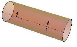
(a)

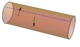
(b)

Figure 1: Riemann surface for finite temperature large interval entanglement entropy. (a): The dashed line is the branch cut, and the arrow indicates the field transforming from the $j$th to the $(j+1)$th replica. (b): The modified branch cut. Note that one should identify the two ends of the cylinder to get a torus.

III Second proof

If we quantize the theory along the spacial direction, the density matrix is of the form

$$\rho_{s}=e^{-RH_{s}}=e^{-\frac{2\pi R}{\beta}}(L_{0}+\widetilde{L_{0}}-\frac{c}{12}).$$ (14)

In this case, we need to cut the thermal cycle and insert a complete set of bases there. However if we cut the thermal cycle across the branch cut, due to the presence of the interval, the field satisfies nontrivial monodromy condition. This requires us to insert a complete basis of twist sector states.

Suppose that one of the branch points is at the origin, then the field satisfies the twist boundary condition

$$\phi^{(j)}(ze^{2\pi i},\bar{z}e^{-2\pi i})=\phi^{(j+1)}(z,\bar{z}),$$ (15)

with $j=1,\cdots,n$ labeling the sheets, and $\phi$ can be any field in a CFT. We can redefine other $n$ fields as

$$\phi^{(t,k)}(z,\bar{z})=\sum_{j=1}^{n}e^{\frac{2\pi i}{n}kj}\phi^{(j)}(z,\bar{z})$$ (16)

with the monodromy condition

$$\phi^{(t,k)}(ze^{2\pi i},\bar{z}e^{-2\pi i})=\phi^{(t,k)}(z,\bar{z})e^{-\frac{2\pi ik}{n}}.$$ (17)

The mode expansion of the field in the twist sector is

$$\phi^{(t,k)}=\frac{1}{n^{h+\bar{h}-1}}e^{\frac{2\pi i}{n}k}\sum_{\begin{subarray}{c}m=-h+s,\bar{m}=-\bar{h}+\bar{s}\\ m-\bar{m}=k+an\end{subarray}}\frac{\phi_{m}\bar{\phi}_{\bar{m}}}{z^{h+\frac{m}{n}}\bar{z}^{\bar{h}+\frac{\bar{m}}{n}}}$$

The lowest state in the twist sector is

$$\phi_{-h}\bar{\phi}_{-\bar{h}}\mid t\rangle,$$ (18)

with the conformal dimension $(\frac{h}{n}+\frac{c}{24}(1-\frac{1}{n^{2}}),\frac{\bar{h}}{n}+\frac{c}{24}(1-\frac{1}{n^{2}})$. Here $\mid t\rangle$ is the twist vacuum with conformal dimension $h=\frac{c}{24}n(1-\frac{1}{n^{2}})$, and the higher conformal dimension states can be built by acting creation operators on this state. There is a one-to-one correspondence between the twist sector states and normal sector states, with their energies being related byChenWu2

$$H = \frac{2\pi}{\beta}(L_{twist}+\tilde{L}_{twist}-\frac{nc}{12})=\frac{H_{normal}}{n}.$$ (19)

With this correspondence, let us discuss the relation (3) again. The partition function $Z_{1}$ is now

$$Z_{1}=e^{R\frac{2\pi}{\beta}\frac{c}{12}}\sum_{i}e^{-\frac{2\pi R}{\beta}\Delta_{i}}.$$ (20)

For the partition function on an $n$-sheeted Riemann surface, we have

$$Z_{n} = e^{\frac{\pi c}{6n}\frac{R}{\beta}}\sum_{i}\langle t,i\mid{\cal{T}}^{-}(-\frac{l}{2}){\cal{T}}^{+}(\frac{l}{2})\mid t,i\rangle e^{-\frac{2\pi R}{n\beta}\Delta_{i}},$$

where the label $t$ denotes the twist sector, and the summation is over all the states in the twisted sector. As the branch points are near each other, we can still use the OPE of the twist operators (9), from which we find

$$S_{n} = -\frac{1}{n-1}\left(\frac{\pi c}{6n}\frac{R}{\beta}+\log~{}(c_{n}l^{-\frac{c}{6}(n-\frac{1}{n})})+\log(\sum_{i}e^{-\frac{2\pi R}{n\beta}\Delta_{i}})\right.$$

$$\left.-n(\frac{\pi c}{6}\frac{R}{\beta}+\log(\sum_{i}e^{-\frac{2\pi R}{\beta}\Delta_{i}})+O(l))\right).$$

Consequently, we have

$$\lim_{l\rightarrow 0}(S_{EE}(R-l)-S_{EE}(l))$$ (21)

$$= \frac{\pi c}{3}\frac{R}{\beta}+\log Z[\frac{R}{\beta}]+\frac{R}{\beta}\frac{Z^{{}^{\prime}}[\frac{R}{\beta}]}{Z[\frac{R}{\beta}]}.$$

The thermal entropy is now

$$S_{th}=\frac{1}{3}\pi c\frac{R}{\beta}+\log Z[\frac{R}{\beta}]+\frac{R}{\beta}\frac{Z^{{}^{\prime}}[\frac{R}{\beta}]}{Z[\frac{R}{\beta}]},$$ (22)

which is the same as (21). This completes our second proof of the relation (3).

In the large central charge limit, the first term in (21) gives the entropy of the BTZ black hole in the bulk, which is dual to the CFT at high temperature. The remaining terms correspond to the quantum corrections. However, we would like to emphasize again that the relation (21) is valid for all temperatures. It is equal to the relation (13), both of which give the thermal entropy of the CFT.

IV A counter-example?

In the above proof, we have assumed that the CFT has a discrete spectrum. It would be interesting to see if the relation (3) is still true for the CFT with a continuous spectrum. Here we discuss the relation for a non-compact free scalarcomment1 . The partition function of this case has been given in terms of $W$ functions in Datta . One may compute the large and short interval expansions of the partition function and check the relation directly, as discussed carefully in ChenWu2 . In the large interval expansion, there appears a term of the form $\log(|\log l|)$, which could not be canceled by the short interval terms. The reason for such a term can be found in the discussion above. One essential point in the above proofs is to use the OPE of the twist operators. However, in the case of a noncompact scalar, the OPE relation (9) breaks down. Actually, the relation changes to

$${\cal{T}}^{+}(-\frac{l}{2}){\cal{T}}^{-}(\frac{l}{2})$$

$$= c_{n}l^{-\frac{1}{6}n(1-\frac{1}{n^{2}})}\left\{V^{n-1}\int\prod_{j=1}^{n}dk_{j}\delta(\sum_{j=1}^{n}k_{j})\right.$$

$$\cdot\prod_{j=1}^{n}(\frac{l}{n})^{2k_{j}^{2}}e^{-ik_{j}\phi^{(j)}(u)}\mid_{u=0}$$

$$\left.\cdot\prod_{1\leq j_{1}<j_{2}\leq n}(2\sin\frac{\pi}{n}(j_{2}-j_{1}))^{2k_{j_{1}}k_{j_{2}}}+O(l)\right\}.$$

where V is the regularized volume in the target space. We regard the non-compact boson as a large volume limit of a compact boson; therefore, we have

$$\sum_{k}\rightarrow\frac{V}{2\pi}\int dk,~{}~{}~{}\delta_{k_{1},k_{2}}\rightarrow\frac{2\pi}{V}\delta(k_{1}-k_{2}),~{}~{}~{}\delta(0)=\frac{V}{2\pi}.$$ (23)

Different from the small interval case, the operators $\displaystyle{\prod_{j=1}^{n}e^{ik_{j}\phi^{(j)}}}$ contribute to the partition function in the large interval limit. In the end, we find that

$$\lim_{l\rightarrow 0}S_{EE}(R-l)-S_{EE}(l)=\log(|\log l|)+S_{th}+c_{1},$$

where $c_{1}=1+\log 4\pi-2\log V$. This result could be obtained by direct expansion of the $W$ functions in the partition function as wellChenWu2 . Actually in getting this result, we have always taken the $V\to\infty$ limit first and then $l\to 0$ such that the theory has a continuous spectrum. The log-logarithmic divergence stems from the continuous spectrum of the non-compact scalar.

In the above discussion, we treat the noncompact free scalar directly, which is gapless and has a continuous spectrum. However, if we start from a compact free scalar with radius $V$ and study the universal relation (3), and finally take $V\to\infty$ limit, then the perplexing term $\log(|\log l|)$ does not appear. Actually, as shown in Chen:2015cna , the universal relation (3) indeed holds for the compact free scalar. Therefore, once we take the noncompact free scalar as a limiting case of compact free scalar, the universal relation still holds.

V Conclusion and discussion

In this letter, we proved the universal relation (3) between the thermal entropy and entanglement entropy for the CFTs with a discrete spectrum. We also discussed this relation for noncompact free scalar with a continuous spectrum and found that there was a subtle order-of-limits issue. If we regularize the theory and take limits in the correct order, the relation still holds. One interesting issue is to check if the relation (3) could be true for a generic 2D quantum field theory without conformal symmetry.

In higher dimensions, the recent study on the holographic entanglement entropy suggests that the Araki-Lieb inequality could be saturated, which is called the entropy plateauHubeny:2013gta . This suggests that there exists some kind of generalization of the relation (3) in higher dimensions. It would be interesting to study such a relation directly in the field theory.

Acknowledgments The work was supported in part by NSFC Grant No. 11275010, No. 11335012, and No. 11325522.

References

- (1) M. A. Nielsen and I. L. Chuang, Quantum computation and quantum information. Cambridge university press, 2010.
- (2) H. Araki and E. H. Lieb, Commun. Math. Phys. 18, 160 (1970).
- (3) L. Amico, R. Fazio, A. Osterloh and V. Vedral, Rev. Mod. Phys. 80, 517 (2008).
- (4) J. Eisert, M. Cramer and M. B. Plenio, Rev. Mod. Phys. 82, 277 (2010).
- (5) S. Ryu and T. Takayanagi, Phys.Rev.Lett. 96 (2006) 181602.
- (6) S. Ryu and T. Takayanagi, JHEP 0608 (2006) 045.
- (7) T. Hartman, “Entanglement Entropy at Large Central Charge,” arXiv:1303.6955 [hep-th].
- (8) T. Faulkner, “The Entanglement Renyi Entropies of Disjoint Intervals in AdS/CFT,” arXiv:1303.7221 [hep-th].
- (9) J. Callan, Curtis G. and F. Wilczek, Phys.Lett. B333 (1994) 55–61.
- (10) P. Calabrese and J. Cardy, J.Phys. A42 (2009) 504005.
- (11) T. Azeyanagi, T. Nishioka and T. Takayanagi, Phys. Rev. D77 (2008) 064005.
- (12) V. E. Hubeny, H. Maxfield, M. Rangamani and E. Tonni, JHEP 1308, 092 (2013).
- (13) Shouvik Datta and Justin R. David, JHEP 1404 (2014) 081.
- (14) B. Chen and Jie-qiang Wu, “Large Interval Limit of Rényi Entropy At High Temperature”, arXiv:1412.0763 [hep-th].
- (15) John Cardy and Christopher P. Herzog, Phys. Rev. Lett. 112,(2014) 171603.
- (16) Bin Chen and Jie-qiang Wu, JHEP 1408, 032 (2014).
- (17) Our discussion is different from the one in Datta , which based on an incorrect relation between functions in the partition function.
- (18) B. Chen and J. q. Wu, “Rényi Entropy of Free Compact Boson on Torus,” arXiv:1501.00373 [hep-th].