Modular decomposition and analysis of biological networks

Abstract

This paper addresses the decomposition of biochemical networks into functional modules that preserve their dynamic properties upon interconnection with other modules, which permits the inference of network behavior from the properties of its constituent modules. The modular decomposition method developed here also has the property that any changes in the parameters of a chemical reaction only affect the dynamics of a single module. To illustrate our results, we define and analyze a few key biological modules that arise in gene regulation, enzymatic networks, and signaling pathways. We also provide a collection of examples that demonstrate how the behavior of a biological network can be deduced from the properties of its constituent modules, based on results from control systems theory.

Keywords:

Systems biology, Modularity, Modular decomposition, Retroactivity, Control Theory

1 Introduction

Network science and control systems theory have played a significant role in the advancement of systems and synthetic biology in recent years. Tools from graph theory and system identification have been used to understand the basic subunits or “motifs” in biological networks [1, 2], and to identify the existence (or non-existence) of pathways in large networks [3, 4, 5]. With a deeper understanding of mechanisms that exist in biology, synthetic biologists have used bottom-up construction techniques to engineer new biological networks, and modify or optimize the behavior of existing networks [6, 7], with impressive results [8, 9, 10].

Modularity

One of the key ideas that has revolutionized synthetic and systems biology is the conception of a biological network as a collection of functionally isolated interacting components. To the authors’ knowledge, Hartwell et al. were among the first to suggest that this idea could reduce the complexity of analyzing these networks [11]. For example, properties like stability and robustness can be predicted just from properties of each individual component in the network and knowledge of the interconnection structure. From a computational perspective, computing network parameters such as its equilibrium point(s) can be greatly simplified, since the computations can be done over a set of components as opposed to over the entire network. From an evolutionary standpoint, grouping a network into components is useful to analyze the evolvability of each component. Finally, for experimental identification purposes, delimiting a network into components reduces the complexity of the estimation problem and often requires less experimental data.

It is generally understood that to be useful, a biological component needs to exhibit a property broadly defined as modularity, but there is little consensus on its definition and on how it is perceived [12]. Synthetic biologists and mathematical biologists postulate that a biological component exhibits modularity if its dynamic characteristics remain the same before and after interconnection with other components [12]. However, synthetic biologists sometimes argue that modularity is not an inherent property of biological network components, because often components have dynamics that are susceptible to change upon interconnection with other components. This has been termed many things, including “hidden feedback” [13], “retroactivity” [14] and “loading effects” [15], and is akin to an electrical component whose output voltage changes upon the addition of a load. To obviate this lack of modularity and to effectively isolate two or more synthetic components from each other, insulation components have been designed [14, 16] and have proven to be useful [17].

Mathematical biologists on the other hand, believe that the fact that some synthetic components can be subject to loading effects upon interconnection with other components provides no reason to believe that biological networks cannot be analytically delimited into components that exhibit modularity. In this field, a biological network is generally represented by a system of ordinary differential equations (ODEs). Every one of these equations is then assigned to a component, with appropriate input-output relationships to ensure that the composition of all components will reconstruct the original system of ODEs. This method of decomposing a biological network has proven useful in deriving results pertaining to the existence of multiple equilibrium points in a network of interconnected components [18, 19, 20], and the stability of these points [21, 22]. A potentially undesirable feature of the approaches followed in the above-mentioned references is that, while the components considered were dynamically isolated from each other, the parameters of a particular chemical reaction in the network (such as the stoichiometric coefficients or the rate constants) could appear in more than one component. Consequently, a change in a single chemical reaction could result in several distinct components changing their internal dynamics.

Evolutionary biologists themselves have different perspectives on modularity. One is that modularity is an inherent property of biological network components that enables them to evolve independently from the rest of the network in response to shock or stress, hence enhancing future evolvability. [23, 24]. Another perspective is that natural selection occurs modularly, and that this selection preserves certain properties of a biological network by allowing individual aspects of a component to be adjusted without negative effects on other aspects of the phenotype. Whichever definition is used, evolutionary biologists rely heavily on biological network parameters being associated with a unique component. For example, parameters that are ”internal” to a functional biological component, but that do not affect significantly the input-output behavior of the component, are considered as neutral traits [25], meaning that their values can change because of genetic drift.

Two notions of modularity

In this paper, we attempt to unify the notion of modularity in the context of biological networks, using an analytical approach. We say that a biological component is a module if it admits both dynamic modularity and parametric modularity. The former implies that the properties of each module do not change upon interconnection with other modules, and the latter implies that the network parameters within a module appear in no other module. In this sense, a synthetic component that undergoes loading effects upon interconnection with other components does not exhibit dynamic modularity, and a component whose internal dynamics depend on parameters that also affect other components does not exhibit parametric modularity.

Dynamic modularity is essential to infer the behavior of a biological network from the behavior of its constituent parts, which can enable the analyses of large networks and also the design of novel networks. Parametric modularity, which has not been explicitly mentioned as often in the literature, is a useful property when identifying parameters in a biological network, like in [3, 4, 5], and also for evolutionary analysis of network modules.

Novel contributions

A key contribution of this paper is the development of a systematic method to decompose an arbitrary network of biochemical reactions into modules that exhibit both dynamic and parametric modularity. This method is explained in detail in Section 2 and is based on three rules that specify how to partition species and reactions into modules and also how to define the signals that connect the modules. An important novelty of our approach towards a modular decomposition is the use of reaction rates as the communicating signals between modules (as opposed to species concentrations). We show that aside from permitting parametric modularity, this allows the use of summation junctions to combine alternative pathways that are used to produce or degrade particular species.

To illustrate the use of our approach, in Section 3 we introduce some key biological modules that arise in gene regulatory networks, enzymatic networks, and signaling pathways. Several of these biological systems have been previously regarded in the literature as biological ”modules”, but the ”modules” proposed before did not simultaneously satisfy the dynamic and parametric modularity properties. We then analyze these modules from a systems theory perspective. Specifically, we introduce the Input-output static characteristic function (IOSCF) and the Linearized Transfer Function (LTF), and explain how these functions can help us characterize a module by properties such as monotonicity and stability.

Section 4 is devoted to demonstrating how one can predict the behavior of large networks from basic properties of its constituent modules. To this effect, we review three key basic mechanisms that can be used to combine simple modules to obtain arbitrarily complex networks: cascade, parallel, and feedback interconnections. We then illustrate how modular decomposition can be used to show that the Covalent Modification network [26] can only admit a single stable equilibrium point no matter how the parameters of the network are chosen, and to find parameter regions where the Repressilator network [9] converges to a stable steady-state.

2 Modularity and Decomposition

From this paper’s perspective, a biological network is viewed as a collection of elementary chemical reactions, whose dynamics are obtained using the law of mass action kinetics. Our goal is to decompose such a network into a collection of interacting modules, each a dynamical system with inputs and outputs, so that the dynamics of the overall network can be obtained by appropriate connections of the inputs and outputs of the different modules that comprise the network. It is our expectation that the decomposition of a biological network into modules will reduce the complexity of analyzing network dynamics, provide understanding on the role that each chemical species plays in the function of the network, and permit accurate predictions regarding the change of behavior that would arise from specific changes to components of the network.

For a network to be truly modular, we argue that the different modules obtained from such a decomposition should exhibit both dynamic modularity and parametric modularity. A module exhibits dynamic modularity if its dynamics remain unchanged upon interconnection with other modules in the network, and admits parametric modularity if the parameters associated with that module appear in no other module of the network. Consequently, changing the parameters of a single chemical reaction affects the dynamics of only a single module.

In the rest of this section, we develop rules that express conditions for a module to admit dynamic and parametric modularity. To express these rules, we introduce a graphical representation that facilitates working with large biological networks.

2.1 Representing a biological network

A biological network can be represented in multiple ways, including as a system of ordinary differential equations (ODEs) associated with the law of mass action kinetics, a directed bipartite species-reaction graph (DBSR), or a dynamic DBSR graph that we introduce below.

Mass Action Kinetics (MAK) Ordinary Differential Equations (ODEs)

A set of species involved in chemical reactions can be expressed as a system of ODEs using the law of mass action kinetics (MAK) when the species are well-mixed and their copy numbers are sufficiently large. For a network involving the species $\mathcal{S}_{j}$, $\forall j\in\{1,2,\dots,N_{\mathrm{species}}\}$ and the reactions $\mathcal{R}_{i}$, $\forall i\in\{1,2,\dots,N_{\mathrm{reactions}}\}$, the MAK results in a system of ODEs whose states are the concentrations $\left[\mathcal{S}_{j}\right]$, $\forall j$ of the different chemical species; the ODE representing the dynamics of a specific species $\mathcal{S}_{j}$ is given by

$$\dot{\left[\mathcal{S}_{j}\right]}=\sum\limits_{i=1}^{N_{\mathrm{reactions}}}\psi_{ji}(k_{1},k_{2},\dots,\left[\mathcal{S}_{1}\right],\left[\mathcal{S}_{2}\right],\dots)$$ (1)

where $\psi_{ji}(k_{1},k_{2},\dots,\left[\mathcal{S}_{1}\right],\left[\mathcal{S}_{2}\right],\dots)$ denotes the rate of production/destruction of $\mathcal{S}_{j}$ due to the reaction $\mathcal{R}_{i}$, which typically depends on the parameters $k_{1},k_{2},\dots$ that are intrinsic to $\mathcal{R}_{i}$ (reaction rate constants and stoichiometric coefficients) and also on the concentrations of the reactants $\left[\mathcal{S}_{1}\right],\left[\mathcal{S}_{2}\right]\cdots$ of $\mathcal{R}_{i}$. The value of $\psi_{ji}$ is either positive or negative depending on whether $\mathcal{S}_{j}$ is produced or consumed (respectively) by $\mathcal{R}_{i}$, or zero if $\mathcal{R}_{i}$ is not involved in the production or consumption of $\mathcal{S}_{j}$.

To facilitate the discussion, we use as a running example a simple biological network consisting of species $\mathcal{S}_{1}$, $\mathcal{S}_{2}$, and $\mathcal{S}_{3}$, represented by the following set of chemical reactions:

$$\centering\begin{aligned} \mathcal{R}_{1}:\mathcal{S}_{1}&\xrightarrow{k_{1}\left[\mathcal{S}_{1}\right]}\mathcal{S}_{2}\\ \mathcal{R}_{2}:\mathcal{S}_{1}&\xrightarrow{\gamma_{1}\left[\mathcal{S}_{1}\right]}\varnothing\end{aligned}\qquad\begin{aligned} \mathcal{R}_{3}:\mathcal{S}_{2}&\xrightarrow{k_{2}\left[\mathcal{S}_{2}\right]}\mathcal{S}_{1}\\ \mathcal{R}_{4}:\mathcal{S}_{2}&\xrightarrow{\gamma_{2}\left[\mathcal{S}_{2}\right]}\varnothing\end{aligned}\qquad\begin{aligned} \mathcal{R}_{5}:\mathcal{S}_{3}&\xrightarrow{k_{3}\left[\mathcal{S}_{3}\right]}\mathcal{S}_{2},\end{aligned}\@add@centering$$ (2)

which correspond to the following set of ODEs derived from MAK:

$$\dot{\left[\mathcal{S}_{1}\right]} =k_{2}\left[\mathcal{S}_{2}\right]-(\gamma_{1}+k_{1})\left[\mathcal{S}_{1}\right]$$ (3a)

$$\dot{\left[\mathcal{S}_{2}\right]} =k_{1}\left[\mathcal{S}_{1}\right]+k_{3}\left[\mathcal{S}_{3}\right]-(\gamma_{2}+k_{2})\left[\mathcal{S}_{2}\right]$$ (3b)

$$\dot{\left[\mathcal{S}_{3}\right]} =-k_{3}\left[\mathcal{S}_{3}\right].$$ (3c)

With respect to the general model (1), the $\psi_{ji}$ for $j\in\{1,2,3\}$ and $i\in\{1,2,3,4,5\}$ are given by

$$\begin{aligned} \psi_{11}\big{(}k_{1},\left[\mathcal{S}_{1}\right]\big{)}&=-k_{1}\left[\mathcal{S}_{1}\right]\\ \psi_{12}\big{(}\gamma_{1},\left[\mathcal{S}_{1}\right]\big{)}&=-\gamma_{1}\left[\mathcal{S}_{1}\right]\\ \psi_{13}\big{(}k_{2},\left[\mathcal{S}_{2}\right]\big{)}&=k_{2}\left[\mathcal{S}_{2}\right]\end{aligned}\qquad\begin{aligned} \psi_{21}\big{(}k_{1},\left[\mathcal{S}_{1}\right]\big{)}&=k_{1}\left[\mathcal{S}_{1}\right]\\ \psi_{23}\big{(}k_{2},\left[\mathcal{S}_{2}\right]\big{)}&=-k_{2}\left[\mathcal{S}_{2}\right]\\ \psi_{24}\big{(}\gamma_{2},\left[\mathcal{S}_{2}\right]\big{)}&=-\gamma_{2}\left[\mathcal{S}_{2}\right]\\ \psi_{25}\big{(}k_{3},\left[\mathcal{S}_{3}\right]\big{)}&=k_{3}\left[\mathcal{S}_{3}\right]\end{aligned}\qquad\begin{aligned} \psi_{35}\big{(}k_{3},\left[\mathcal{S}_{3}\right]\big{)}=-k_{3}\left[\mathcal{S}_{3}\right],\end{aligned}$$

and $0$ otherwise.

Directed Bipartite Species-Reactions (DBSR) graph

When a biological network is large, writing down the system of MAK ODEs is cumbersome and therefore much work has been done on understanding the behavior of chemical reaction networks from a graph-theoretic perspective [27]. The Directed Bipartite Species-Reaction (DBSR) graph representation of chemical reaction networks was developed in [28], and is closely related to the Species-Reaction (SR) graph introduced in [29]. In the construction of the DBSR graph, every species in the network is assigned to an elliptical node, and every chemical reaction is assigned to a rectangular node. For every reaction in the network $\mathcal{R}_{i}$, there exist directed edges from the nodes corresponding to the reactants of $\mathcal{R}_{i}$ to the node $\mathcal{R}_{i}$, and from the node $\mathcal{R}_{i}$ to the nodes corresponding to the products of $\mathcal{R}_{i}$. It is worth noting that this formulation is similar to that in [30], using storages and currents. The DBSR graph of the network (2) is shown in Figure 1(a). From this graph, we can infer, for example, that $\mathcal{S}_{2}$ is produced from $\mathcal{S}_{1}$ due to the reaction $\mathcal{R}_{1}$, and that $\mathcal{S}_{1}$ is a reactant in $\mathcal{R}_{1}$. Therefore, the concentration of $\mathcal{S}_{1}$ is required in the computation of the rate of the reaction $\mathcal{R}_{1}$.

(a)

(b)

Figure 1: 1(a) DBSR graph and 1(b) Dynamic DBSR graph of the network represented by (2)

Dynamic DBSR graph

While the DBSR graph is useful in understanding the overall structure of a network of chemical reactions, it does not provide information about the flow of information in the network. For instance, the graph does not directly show whether the reaction $\mathcal{R}_{1}$ affects the dynamics of $\mathcal{S}_{1}$. To obviate this problem, we define the dynamic DBSR graph, which is a DBSR graph overlaid with arrows expressing the flow of information due to the dynamics of the network. In this graph, a dashed arrow from a reaction node $\mathcal{R}_{i}$ to a product node $\mathcal{S}_{j}$ indicates that $\left[\mathcal{S}_{j}\right]$ is affected by $\mathcal{R}_{i}$, usually by $\mathcal{S}_{j}$ being consumed in the reaction. Just like in the DBSR graph, a solid arrow from node $\mathcal{R}_{i}$ to node $\mathcal{S}_{j}$ indicates that $\mathcal{S}_{j}$ is produced by the reaction, while a solid arrow from node $\mathcal{S}_{j}$ to node $\mathcal{R}_{i}$ indicates that $\mathcal{S}_{j}$ is a reactant of $\mathcal{R}_{i}$. The Dynamic DBSR graph of network (2) is shown in Figure 1(b).

2.2 Modular decomposition of a biological network

The modular decomposition of a biological network represented by the MAK ODE (1) entails the assignment of each chemical species and each chemical reaction in the network to modules. These modules then need to be interconnected appropriately such that the ODE (1) can be reconstructed from the module dynamics. In our framework, the assignment of a chemical species $\mathcal{S}_{j}$ to a module means that the species concentration $\left[\mathcal{S}_{j}\right]$ is part of the state of that module alone. The assignment of a chemical reaction to a module means that all the reaction parameters (such as stoichiometric coefficients and rate constants) appear only in that module. These observations lead to the formulation of two rules for a modular decomposition:

Rule 1 (Partition of species)

Each chemical species $\mathcal{S}_{j}$ must be associated with one and only one module $\mathcal{M}$, and the state of $\mathcal{M}$ is a vector containing the concentrations of all chemical species associated with $\mathcal{M}$. $\Box$

Rule 2 (Partition of reactions)

Each chemical reaction $\mathcal{R}$ must be associated with one and only one module $\mathcal{M}$, and the stoichiometric parameters and rate constants associated with $\mathcal{R}$ must only appear within the dynamics of module $\mathcal{M}$. $\Box$

In terms of the DBSR graphs, Rules 1 and 2 express that each node in the graph (corresponding to either a species or a reaction) must be associated with a single module. Therefore, our modular decomposition can be viewed as a partition of the nodes of the DBSR graphs. We recall that a partition of a graph is an assignment of the nodes of the graph to disjoint sets.

The choice of signals used to communicate between modules has a direct impact on whether or not Rules 1 and 2 are violated. To understand why this is so, consider again the biological network (2), corresponding to the MAK ODEs given by (3), and suppose that we want to associate each of the three species $\mathcal{S}_{1}$, $\mathcal{S}_{2}$ and $\mathcal{S}_{3}$ with a different component. Figure 2 shows two alternative partitions of the network that satisfy Rule 1 and exhibit the dynamic modularity property. That is, the concentration of each species appears in the state of one and only one component, and when the three components are combined, we obtain precisely the MAK ODEs in (3).

(a) Decomposition using species concentrations as inputs and outputs, which satisfies Rule 1, but not Rule 2.

(b) Decomposition using production rates as inputs and outputs, which satisfies Rules 1 and 2.

(c) DBSR graph partition corresponding to the decomposition in Figure 2(b).

Figure 2: Modular decomposition of the biochemical network (2) corresponding to the dynamic DBSR graph in Figure 1(b).

In the decomposition depicted in the block diagram in Figure 2(a), the communicating signals are the concentrations of the species. Specifically, the outputs $y_{1}$, $y_{2}$, and $y_{3}$ of components $\mathcal{M}_{1}$, $\mathcal{M}_{2}$, and $\mathcal{M}_{3}$, respectively, are the concentrations of the species $\mathcal{S}_{1}$, $\mathcal{S}_{2}$, and $\mathcal{S}_{3}$; which in turn are the inputs $u_{2}$, $u_{1}$, or $u_{3}$ of components $\mathcal{M}_{2}$, $\mathcal{M}_{1}$, and $\mathcal{M}_{3}$, respectively. This type of decomposition, where species concentrations are used as communicating signals between modules, has been commonly done in the literature [31, 15, 30, 32, 33]. However, this decomposition violates Rule 2, because the rate parameters of the reactions $\mathcal{R}_{1}$, $\mathcal{R}_{3}$, and $\mathcal{R}_{5}$ appear in multiple components. Consequently, this partition does not exhibit parametric modularity; for example, a change in the rate constant $k_{3}$ for reaction $\mathcal{R}_{5}$ would change the internal dynamics of modules $\mathcal{M}_{2}$ and $\mathcal{M}_{3}$. We thus do not refer to the components $\mathcal{M}_{1}$, $\mathcal{M}_{2}$, and $\mathcal{M}_{3}$ in Figure 2(a) as “modules.”

An alternative choice for the communicating signals would be the rates of production of the species, which leads to the decomposition depicted in the block diagram in Figure 2(b). With this decomposition, we can now partition both the species and the reaction nodes among the different components so that the parameters of each reaction are confined to a single module, as illustrated in Figure 2(c). We thus have a modular decomposition that simultaneously satisfies Rules 1 and 2 and refer to the components $\mathcal{M}_{1}$, $\mathcal{M}_{2}$, and $\mathcal{M}_{3}$ in Figure 2(b) as “modules.”

2.3 Rates as communicating signals

In the context of a simple example, we have seen that using rates as the communicating signals between modules (as opposed to protein concentrations) enables a modular decomposition that simultaneously satisfies Rules 1 and 2. We now generalize these ideas to arbitrary biological networks.

When partitioning a dynamic DBSR graph into modules, each arrow of the graph “severed” by the partition corresponds to an interconnecting signal flowing between the resulting modules, in the direction of the arrow. For example, one can see two arrows being severed in Figure 2(c) by the partition between modules $\mathcal{M}_{1}$ and $\mathcal{M}_{2}$ and then two signals ($y_{2}$ and $y_{1}$) connecting the corresponding modules in Figure 2(b). In the remainder of this section, we present two basic scenarios that can arise in partitioning a network into two modules and discuss the signals that must flow between these modules. These two cases can be applied iteratively to partition a general network into an arbitrary number of modules.

Partition at the output of a reaction node.

(a) Dynamic DBSR graph partition

(b) Block diagram decomposition.

Figure 3: Modular decomposition corresponding to the partition of a biochemical network at the output of a reaction node of the dynamic DBSR graph.

Suppose first that we partition a biological network into two modules $\mathcal{M}_{1}$ and $\mathcal{M}_{2}$ at the output of a reaction node of the dynamic DBSR graph, corresponding to a generic elementary reaction of the form

$$\mathcal{R}_{1}:\mathcal{S}_{1}+\mathcal{S}_{2}\xrightarrow{k\left[\mathcal{S}_{1}\right]\left[\mathcal{S}_{2}\right]}\mathcal{S}_{3},$$ (4)

as shown in Figure 3(a). This can be accomplished by connecting an output $y_{1}$ from module $\mathcal{M}_{1}$ to an input $u_{2}$ of module $\mathcal{M}_{2}$ that is equal to the rate of production of $\mathcal{S}_{3}$ due to $\mathcal{R}_{1}$, which is given by $k\left[\mathcal{S}_{1}\right]\left[\mathcal{S}_{2}\right]$. The block diagram representation of this partition is shown in Figure 3(b). In this configuration, the reaction rate parameter $k$ only appears inside the module $\mathcal{M}_{1}$ and we thus have parametric modularity. As far as $\mathcal{M}_{2}$ is concerned, the rate of production of $\mathcal{S}_{3}$ in molecules per unit time is given by the abstract chemical reaction

$$\varnothing\xrightarrow{u_{1}}\mathcal{S}_{3},$$

where the rate $u_{1}$ is an input to the module. In this decomposition, we also have dynamic modularity, since when we combine the dynamics of the two modules in Figure 3(b), we recover the MAK ODEs. This partition therefore ensures that both Rules 1 and 2 are satisfied. We emphasize that the single arrow from node $\mathcal{R}_{1}$ to node $\mathcal{S}_{3}$ that is “severed” by the partition in Figure 3(a), gives rise to one signal flowing from $\mathcal{M}_{1}$ to $\mathcal{M}_{2}$ in Figure 3(b).

(a) Dynamic DBSR graph partition

(b) Block diagram decomposition.

Figure 4: Modular decomposition corresponding to the partition of a biochemical network at the output of a species node of the dynamic DBSR graph.

Partition at the input of a reaction node.

Now consider the case where we partition the network at an input of a reaction node of the dynamic DBSR graph, corresponding to a generic elementary reaction of the form in (4), as shown in Figure 4(a). This can be accomplished by a bidirectional connection between the two modules: The output $y_{1}$ from $\mathcal{M}_{2}$ is connected to the input $u_{1}$ of $\mathcal{M}_{1}$ and is equal to $k\left[\mathcal{S}_{2}\right]$, which is the degradation rate of a single molecule of $\mathcal{S}_{1}$ due to the reaction $\mathcal{R}_{1}$, in molecules per molecule of $\mathcal{S}_{1}$ per unit time. The output $y_{2}$ from $\mathcal{M}_{1}$ is connected to the input $u_{2}$ of $\mathcal{M}_{2}$ and is equal to $u_{1}\left[\mathcal{S}_{1}\right]$, which is the rate of production of $\mathcal{S}_{3}$ and the net consumption rate of $\mathcal{S}_{2}$ due to $\mathcal{R}_{1}$, both in molecules per unit time. The block diagram representation of this modular decomposition is shown in Figure 4(b). In isolation, the block $\mathcal{M}_{1}$ corresponds to a chemical reaction of the form

$$\mathcal{S}_{1}\xrightarrow{u_{1}\left[\mathcal{S}_{1}\right]}\varnothing,$$

where the input $u_{1}$ determines the degradation rate of the species $\mathcal{S}_{1}$, and the block $\mathcal{M}_{2}$ corresponds to an abstract chemical reaction of the form

$$\mathcal{S}_{2}\xrightarrow{u_{2}}\mathcal{S}_{3},$$

where the input $u_{2}$ determines the production rate of the species $\mathcal{S}_{3}$, which is also the net consumption rate of $\mathcal{S}_{2}$. This decomposition is parametrically modular since the reaction rate parameter $k$ is only part of the module $\mathcal{S}_{2}$, which contains the reaction $\mathcal{R}_{1}$. We emphasize that the two arrows between $\mathcal{R}_{1}$ to $\mathcal{S}_{1}$ that are “severed” by the partition in the dynamic DBSR in Figure 4(a) give rise to the two signals flowing between $\mathcal{M}_{1}$ and $\mathcal{M}_{2}$ in Figure 4(b).

The discussion above gives rise to the following general rule that governs the communicating signals between modules.

Rule 3 (Communication signals between modules)

Each arrow of the dynamic DBSR graph that is “severed” by the partition that defines the modular decomposition gives rise to one signal that must flow between the corresponding modules. Specifically,

1. When the modular decomposition cuts the dynamic DBSR graph between a reaction node $\mathcal{R}_{i}$ and a product species node $\mathcal{S}_{j}$ at the output of node $\mathcal{R}_{i}$, one signal must flow between the modules: the module with the reaction must have an output equal to the rate [in molecules per unit time] at which the product $\mathcal{S}_{j}$ is produced by the reaction.

2. When the modular decomposition cuts the dynamic DBSR graph between a reaction node $\mathcal{R}_{i}$ and a reactant species node $\mathcal{S}_{j}$ at the output of node $\mathcal{S}_{j}$, two signals must flow between the corresponding modules: the module with the reaction must have an output equal to the rate at which each molecule of $\mathcal{S}_{j}$ is degraded [in molecules per molecule of $\mathcal{S}_{j}$ per unit time], and the module with $\mathcal{S}_{j}$ must have an output equal to the total rate at which the molecules of $\mathcal{S}_{j}$ are consumed [in molecules per unit time]. $\Box$

When Rules 1–3 are followed, the decomposition of the network into modules will exhibit both parametric and dynamic modularity. Furthermore, the network can be decomposed into any number of modules less than or equal to the total number of reacting species in the network.

Remark 1

In exploring the different possible cases, we restricted our discussion to elementary reactions (at most two reactants) and assumed that at least one of the reactants remains in the same module as the reaction. We made these assumptions mostly for simplicity, as otherwise one would have to consider a large number of cases. $\Box$

2.4 Summation Junctions

In biological networks, it is not uncommon for a particular species to be produced or degraded by two or more distinct pathways. In fact, we have already encountered this in the biochemical network (2) corresponding to the dynamic DBSR graph depicted in Figure 1(b), where the species $\mathcal{S}_{2}$ is produced both by reactions $\mathcal{R}_{1}$ and $\mathcal{R}_{5}$. The use of rates as communicating signals between modules allows for the use of summation junctions outside modules to combine different mechanisms to produce/degrade a chemical species.

Figure 5: Modular decomposition from Figure 2(b), simplified using summation junctions.

This is illustrated in Figure 5, where we provide a modular decomposition alternative to that shown in Figure 2(b). This decomposition still preserves the properties of dynamic and parametric modularity, but permits simpler blocks than those in Figure 2(b), since each module now only has a single input and a single output (SISO). As we shall see in Section 4, there are many tools that can be used to analyse interconnections of SISO modules that include external summation junctions.

It is worth noting that when species concentrations are used as the communicating signals between modules [as in Figure 2(a)], it is generally not possible to use summation junctions to combine two or more distinct mechanisms to produce or degrade a chemical species. Even if parametric modularity were not an issue, this limitation would typically lead to more complicated modules with a larger number of inputs and outputs.

3 Common Modules

In this section, we consider a few key biological modules that arise in gene regulatory networks, enzymatic networks, and signaling pathways. We characterize these modules in terms of system theoretic properties that can be used to establish properties of complex interconnections involving these modules. Before introducing the biological modules of interest, we briefly recall some of these system theoretic properties.

3.1 Module properties

Consider a generic input-output module, expressed by an ODE of the form

$$\dot{x} =A(x,u), y =B(x,u), x\in\mathbb{R}^{n},u\in\mathbb{R}^{k},y\in\mathbb{R}^{m},$$ (5)

where $x(t)$ denotes the $n$-vector state of the module, $u(t)$ the $k$-vector input to the module, and $y(t)$ the $m$-vector output from the module.

We say that the module described by (5) is positive if the entries of its state vector $x(t)$ and output vector $y(t)$ never take negative values, as long as all the entries of the initial condition $x(0)$ and of the input vector $u(t)$, $\forall t\geq 0$ never take negative values. All the modules described in this section are positive.

We say that the module described by (5) is cooperative (also known as monotone with respect to the positive orthant) if for all initial conditions $x_{0},\bar{x}_{0}\in\mathbb{R}^{n}$ and inputs $u(t),\bar{u}(t)\in\mathbb{R}^{k}$, $\forall t\geq 0$, we have that

$$x_{0}\gg\bar{x}_{0}\quad \&\quad u(t)\succeq\bar{u}(t),\;\forall t\geq 0\quad\Rightarrow\quad x(t;x_{0},u)\gg x(t;\bar{x}_{0},\bar{u}),\;\forall t>0$$

where $x(t;x_{0},u)$ denotes the solution to (5) at time $t$, starting from the initial condition $x(0)=x_{0}$ and with the input $u$. Given two vectors $v,\bar{v}$, we write $v\gg\bar{v}$ if every entry of $v$ is strictly larger than the corresponding entry of $\bar{v}$ and we write $v\succeq\bar{v}$ if every entry of $v$ is larger than or equal to the corresponding entry of $\bar{v}$. The reader is referred to [18, 19, 20] for a more comprehensive treatment of monotone dynamical systems, including simple conditions to test for monotonicity and results that allow one to infer monotonicity of a complex network from the monotonicity of its constituent parts. Several modules described in this section are cooperative.

The Input-to-State Static Characteristic Function (ISSCF) $g(u^{*})$ of (5) specifies how a constant input $u(t)=u^{*}$, $\forall t\geq 0$ to the module maps to the corresponding equilibrium value of the state $x(t)=x^{*}$, $\forall t\geq 0$. In terms of (5), the value of $g(u^{*})$ is the (unique) solution $x^{*}$ to the steady-state equation $A(x^{*},u^{*})$ = 0. When this equation has multiple solutions $x^{*}$, the ISSCF is not well defined.

For modules with a well-defined ISSCF, the Input-to-Output Static Characteristic Function (IOSCF) $f(u^{*})$ of (5) specifies how a constant input $u(t)=u^{*}$, $\forall t\geq 0$ to the module maps to the corresponding equilibrium value of the output $y(t)=y^{*}$, $\forall t\geq 0$. In terms of (5), the value of $f(u^{*})$ is given by $B(g(u^{*}),u^{*})$. We shall see in Section 4 that one can determine the equilibrium point of a network obtained from the interconnection of several input-output modules like (5), from the IOSCFs and the ISSCFs of the constituent modules.

For systems with a well-defined ISSCF, the Linearized Transfer Function (LTF) $H(s)$ of (5) around an equilibrium defined by the input $u^{*}$ determines how a small perturbation $\delta u(t)\coloneq u(t)-u^{*}$ of the input $u(t)$ around the constant input $u(t)=u^{*}$, $\forall t\geq 0$ leads to a perturbation $\delta y(t)\coloneq y(t)-y^{*}$ of the output $y(t)$ around the constant equilibrium output $y(t)=y^{*}\coloneq f(u^{*})$, $\forall t\geq 0$. In particular, $\delta y(t)=\mathcal{L}^{-1}[H(s)]\star\delta u(t)$, where $\mathcal{L}^{-1}[H(s)]$ denotes the inverse Laplace transform of $H(s)$ and $\star$ the convolution operator [34]. We shall also see in Section 4 that one can determine the LTF of a network obtained from the interconnection of several input-output modules like (5), from the LTFs of the constituent modules.

The LTF of a module like (5) is given by a rational function and generally, the (local) stability of the equilibrium defined by the input $u^{*}$ can be inferred from the roots of the denominator of the LTF. Specifically, if all the roots have strictly negative real parts, in which case we say that the LTF is bounded-input/bounded-output (BIBO) stable, then the equilibrium point is locally asymptotically stable, which means solutions starting close to the equilibrium will converge to it as $t\to\infty$; this assumes that the McMillan degree of the LTF equals the size $n$ of the state $x$ of (5) [34], which is generically true, but should be tested.

3.2 Transcriptional regulation (TR) module

A gene regulatory network consists of a collection of transcription factor proteins, each involved in the regulation of other proteins in the network. Such a network can be decomposed into transcriptional regulation (TR) modules, each containing a transcription factor $\mathcal{S}_{0}$, the promoter regions of a set of genes $\mathcal{G}_{1},\mathcal{G}_{2},\dots,\mathcal{G}_{F}$ that $\mathcal{S}_{0}$ up-regulates or down-regulates, and the corresponding mRNA molecules $mRNA_{1},mRNA_{2},\dots,mRNA_{F}$ transcribed. The case $F>1$ is referred to in the literature as fan-out [35].

The input $u$ to a TR module is the rate of production of $\mathcal{S}_{0}$ due to exogenous processes such as regulation from other TR modules, and can be associated with a generic reaction of the form

$$\varnothing\xrightarrow{u}\mathcal{S}_{0}.$$

A number $q_{j}\geq 1$ of molecules of the transcription factor $\mathcal{S}_{0}$ can bind to the promoter region $P_{j}$ of the gene $\mathcal{G}_{j}$, which is represented by the reaction

$$q_{j}\mathcal{S}_{0}+P_{j} \xrightleftharpoons[k^{\mathrm{off}}_{j}\left[\mathcal{S}_{0}\textup{:}P_{j}\right]]{k^{\mathrm{on}}_{j}\left[\mathcal{S}_{0}\right]^{q_{j}}\left[P_{j}\right]}\mathcal{S}_{0}\textup{:}P_{j},\qquad\forall j\in\{1,2,\dots,m\}.$$

The total concentration of promoter regions $P^{\mathrm{tot}}_{j}=[P_{j}]+[\mathcal{S}_{0}\textup{:}P_{j}]$ for the gene $\mathcal{G}_{j}$ (bound and unbound to the transcription factor) is assumed to remain constant. When $\mathcal{S}_{0}$ activates the gene $\mathcal{G}_{j}$, the bound complex $\mathcal{S}_{0}\textup{:}P_{j}$ gives rise to transcription, which is expressed by a reaction of the form

$$\mathcal{S}_{0}\textup{:}P_{j} \xrightarrow{\alpha_{j}\left[\mathcal{S}_{0}\textup{:}P_{j}\right]}\mathcal{S}_{0}\textup{:}P_{j}+mRNA_{j}.$$

Alternatively, when $\mathcal{S}_{0}$ represses the gene $\mathcal{G}_{j}$, it is the unbounded promoter $P_{j}$ that gives rise to transcription, which is expressed by a reaction of the form

$$P_{j} \xrightarrow{\alpha_{j}\left[P_{j}\right]}P_{j}+mRNA_{j}.$$

Additional reactions in the module include the translation of $mRNA_{j}$ to $\mathcal{S}_{j}$

$$mRNA_{j} \xrightarrow{\beta_{j}\left[mRNA_{j}\right]}mRNA_{j}+\mathcal{S}_{j},$$

and the protein and mRNA degradation reactions

$$\mathcal{S}_{0} \xrightarrow{\bar{\beta}\left[\mathcal{S}_{0}\right]}\varnothing,$$

$$mRNA_{j} \xrightarrow{\gamma_{j}\left[mRNA_{j}\right]}\varnothing$$

The TR module has $F$ outputs $y_{1},y_{2},\dots,y_{F}$ that are equal to the rates of translations of the proteins $\mathcal{S}_{1},\mathcal{S}_{2},\dots,\mathcal{S}_{F}$, respectively. In particular,

$$y_{j}=\beta_{j}\left[mRNA_{j}\right]$$

When $F=1$, we refer to each module simply as a TR activator or TR repressor module, and the subscript $j$’s can be omitted.

Table 1 shows the system of ODEs that correspond to the TR module, as well as its IOSCF and LTF, under the following assumptions:

Assumption 1 (Homogeneity in TR module)

For simplicity of presentation, it is assumed that the association and dissociation constants, the total promoter concentration, and the stoichiometric coefficients are the same for every gene, i.e., that $k^{\mathrm{off}}_{j}=k^{\mathrm{off}}$, $k^{\mathrm{on}}_{j}=k^{\mathrm{on}}$, $P^{\textup{tot}}_{j}=P^{\textup{tot}}$ and $q_{j}=q$, $\forall j\in\{1,2,\dots,F\}$.

Assumption 2 (Parameters in TR module)

The following assumptions on the parameter values are considered:

1. The binding-unbinding reactions are on timescales much faster than those of the transcription, translation, and decay reactions, i.e., $k^{\textup{off}},k^{\textup{on}}\gg\gamma$, $\beta_{j}$, $\bar{\beta}$ and $u(t)$ $\forall t\geq 0$ [14]. This assumption simplifies the LTF of the module, as shown in Table 1.

2. The dissociation constant $K=\frac{k^{\textup{off}}}{k^{\textup{on}}}$ is much higher than the total promoter concentration i.e $K\gg P^{\textup{tot}}$, implying that the affinity of each binding site is small.  $\Box$

An interesting consequence of Assumption 2 is that the LTFs from a perturbation in the input to a perturbation in each of the outputs do not depend on the fan-out, which is not true for the original dynamics without this assumption. For completeness, we include in Appendix A the LTF of the TR module computed without Assumption 2.

	$\mathcal{S}_{0}$ activates $\mathcal{G}_{j}$	$\mathcal{S}_{0}$ represses $\mathcal{G}_{j}$
Dynamics (under Assumption 1)	$\displaystyle\dot{\left[\mathcal{S}_{0}\right]}$ $\displaystyle=u-\bar{\beta}\left[\mathcal{S}_{0}\right]+\sum_{j=1}^{m}q\big{(}k^{\mathrm{off}}\left[\mathcal{S}_{0}\textup{:}P_{j}\right]-k^{\mathrm{on}}\left[\mathcal{S}_{0}\right]^{q}(P^{\mathrm{tot}}-\left[\mathcal{S}_{0}\textup{:}P_{j}\right])\big{)}$ $\displaystyle\dot{\left[\mathcal{S}_{0}\textup{:}P_{j}\right]}$ $\displaystyle=-k^{\mathrm{off}}\left[\mathcal{S}_{0}\textup{:}P_{j}\right]+k^{\mathrm{on}}\left[\mathcal{S}_{0}\right]^{q}(P^{\mathrm{tot}}-\left[\mathcal{S}_{0}\textup{:}P_{j}\right])$
	$\dot{\left[mRNA_{j}\right]}=\alpha_{j}\left[\mathcal{S}_{0}\textup{:}P_{j}\right]-\gamma_{j}\left[mRNA_{j}\right]$	$\dot{\left[mRNA_{j}\right]}=\alpha_{j}(P^{\textup{tot}}-\left[\mathcal{S}_{0}\textup{:}P_{j}\right])-\gamma_{j}\left[mRNA_{j}\right]$
Dynamics (under Assumptions 1–2)	$\displaystyle\dot{\left[\mathcal{S}_{0}\right]}=u-\bar{\beta}\left[\mathcal{S}_{0}\right]$
	$\dot{\left[mRNA_{j}\right]}=\frac{\alpha_{j}P^{\mathrm{tot}}_{j}}{1+\frac{K}{\left[\mathcal{S}_{0}\right]^{q}}}-\gamma_{j}\left[mRNA_{j}\right]$	$\dot{\left[mRNA_{j}\right]}=\frac{\alpha_{j}P^{\mathrm{tot}}_{j}}{1+\frac{\left[\mathcal{S}_{0}\right]^{q}}{K}}-\gamma_{j}\left[mRNA_{j}\right]$
Outputs (under Assumption 1)	$y_{j}=\beta_{j}\left[mRNA_{j}\right]$
IOSCFs (under Assumption 1)	$\displaystyle y_{j}^{*}=\frac{\alpha_{j}\beta_{j}P^{\mathrm{tot}}}{\gamma_{j}\Big{(}1+\frac{K}{(\theta u^{*})^{q}}\Big{)}}$	$\displaystyle y_{j}^{*}=\frac{\alpha_{j}\beta_{j}P^{\mathrm{tot}}}{\gamma_{j}\Big{(}1+\frac{(\theta u^{*})^{q}}{K}\Big{)}}$
LTFs (under Assumptions 1–2)	$\displaystyle H_{j}(s)=\frac{qKP^{\mathrm{tot}}\alpha_{j}\beta_{j}(\theta u^{*})^{q-1}}{(K+(\theta u^{*})^{q})^{2}(s+\gamma_{j})(s+\bar{\beta})}$	$\displaystyle H_{j}(s)=-\frac{qKP^{\mathrm{tot}}\alpha_{j}\beta_{j}(\theta u^{*})^{q-1}}{(K+(\theta u^{*})^{q})^{2}(s+\gamma_{j})(s+\bar{\beta})}$
	where $K\coloneq\frac{k^{\textup{off}}}{k^{\textup{on}}},\qquad\theta=\coloneq\frac{1}{\bar{\beta}}$

Table 1: Dynamics of a transcriptional regulation (TR) module and the corresponding IOSCF and LTF for each type of output. This module is positive and the equilibrium defined by any constant input $u^{*}$ is locally asymptotically stable, under Assumptions 1–2. The module is also cooperative under these assumptions when all outputs are activating.

Figure 6 shows a biological representation and the corresponding DBSR graph of a TR module. The reader may verify from Table 1 that the module satisfies Rules 1–3 in that (i) its state contains the concentrations of all the chemical species associated with the module, (ii) the parameters of all the chemical reactions associated with the module are not needed outside this module, and (iii) the inputs and outputs of the module are rates of protein production/degradation.

(a)

(b)

Figure 6: 6(a) Biological representation and 6(b) DBSR graph of a TR module. For simplicity, protein degradation reactions are shown neither in Figure 6(b) nor in all subsequent DBSR graphs presented in this paper.

3.3 Enzyme-substrate reaction (ESR) module

The enzyme-substrate reaction (ESR) module represents the process by which a substrate protein $\mathcal{S}_{0}$ is covalently modified by an enzyme $E$ into an alternative form $\mathcal{S}_{1}$. The chemical species associated with this module are the substrate protein $\mathcal{S}_{0}$, the enzyme $E$, and the complex $\mathcal{S}_{0}\textup{:}E$ formed by the enzyme-substrate binding. The input $u$ to the ESR module is the rate of production of the substrate $\mathcal{S}_{0}$ due to an exogenous process (e.g., a TR or another ESR module) and can be associated with the generic reaction

$$\varnothing\xrightarrow{u}\mathcal{S}_{0}.$$

The additional reactions associated with the ESR module include the $\mathcal{S}_{0}$ degradation reaction

$$\mathcal{S}_{0}\xrightarrow{\gamma\left[\mathcal{S}_{0}\right]}\varnothing,$$

and the reactions involved in the Michaeles-Menten model for the enzyme-substrate interaction:

$$\mathcal{S}_{0}+E\xrightleftharpoons[k^{\mathrm{r}}\left[\mathcal{S}_{0}\textup{:}E\right]]{k^{\mathrm{f}}\left[\mathcal{S}_{0}\right]\left[E\right]}\mathcal{S}_{0}\textup{:}E\xrightarrow{k^{\mathrm{cat}}\left[\mathcal{S}_{0}\textup{:}E\right]}\mathcal{S}_{1}+E,$$

where the total concentration of enzyme $E^{\mathrm{tot}}=[E]+[\mathcal{S}_{0}\textup{:}E]$ is assumed to remain constant. The output $y$ of the ESR module is the rate of production of the modified substrate $\mathcal{S}_{1}$, given by

$$y=k^{\mathrm{cat}}\left[\mathcal{S}_{0}\textup{:}E\right].$$

Table 2 shows the system of ODEs that correspond to the ESR module, as well as its IOSCF, and LTF. For simplicity, instead of presenting the exact dynamics of the module (which are straighforward to derive using MAK), we present two common approximations to the Michaeles-Menten model:

Assumption 3 (Equilibrium Approximation [36])

The reversible reaction is in thermodynamic equilibrium (i.e., $k^{\textup{f}}\left[\mathcal{S}_{0}\right]\left[E\right]=k^{\textup{r}}\left[\mathcal{S}_{0}\textup{:}E\right]$), which is valid when $k^{\textup{r}}\gg k^{\mathrm{cat}}$. $\Box$

Assumption 4 (Quasi Steady-State Approximation [37])

The concentration of the complex $\mathcal{S}_{0}\textup{:}E$ does not change on the timescale of product formation (i.e., $k^{\textup{f}}\left[\mathcal{S}_{0}\right]\left[E\right]=k^{\textup{r}}\left[\mathcal{S}_{0}\textup{:}E\right]+k^{\textup{cat}}\left[\mathcal{S}_{0}\textup{:}E\right]$), which is valid either when $k^{\mathrm{r}}+k^{\mathrm{cat}}\gg k^{\mathrm{f}}$ or when $\left[\mathcal{S}_{0}\right]\gg E^{\textup{tot}}$. $\Box$

Figure 7 shows a biological representation and the corresponding DBSR graph of an ESR module.

	Equilibrium Approximation (Assumption 3)	Quasi Steady-State Approximation (Assumption 4)
Dynamics	$\dot{\left[\mathcal{S}_{0}\right]}=\frac{u-\gamma\left[\mathcal{S}_{0}\right]-\frac{k^{\textup{cat}}E^{\textup{tot}}\left[\mathcal{S}_{0}\right]}{K^{\mathrm{d}}+\left[\mathcal{S}_{0}\right]}}{1+\frac{K^{\mathrm{d}}E^{\textup{tot}}}{(K^{\mathrm{d}}+\left[\mathcal{S}_{0}\right]^{2})}}$	$\displaystyle\dot{\left[\mathcal{S}_{0}\right]}=u-\gamma\left[\mathcal{S}_{0}\right]-\frac{k^{\mathrm{cat}}E^{\textup{tot}}\left[\mathcal{S}_{0}\right]}{K^{\mathrm{m}}+\left[\mathcal{S}_{0}\right]}$
Output equation	$\displaystyle y=\frac{k^{\mathrm{cat}}E^{\textup{tot}}\left[\mathcal{S}_{0}\right]}{K^{\mathrm{d}}+\left[\mathcal{S}_{0}\right]}$, $\displaystyle K^{\mathrm{d}}\coloneq\frac{k^{\mathrm{r}}}{k^{\mathrm{f}}}$	$\displaystyle y=\frac{k^{\mathrm{cat}}E^{\textup{tot}}\left[\mathcal{S}_{0}\right]}{K^{\mathrm{m}}+\left[\mathcal{S}_{0}\right]}$, $\displaystyle K^{\mathrm{m}}\coloneq\frac{k^{\mathrm{r}}+k^{\mathrm{cat}}}{k^{\mathrm{f}}}$
IOSCF	$\displaystyle y^{*}=\frac{1}{2}(2u^{*}+K^{\mathrm{e}}-\sqrt{(K^{\mathrm{e}})^{2}+4K^{\mathrm{d}}u^{*}\gamma})$, $K^{\mathrm{e}}\coloneq-u^{*}+k^{\mathrm{cat}}E^{\textup{tot}}+K^{\mathrm{d}}\gamma$	$\displaystyle y^{*}=\frac{1}{2}(2u^{*}+K^{\mathrm{f}}-\sqrt{(K^{\mathrm{f}})^{2}+4K^{\mathrm{m}}u^{*}\gamma})$, $K^{\mathrm{f}}\coloneq-u^{*}+k^{\mathrm{cat}}E^{\textup{tot}}+K^{\mathrm{m}}\gamma$
LTF	$\displaystyle H(s)=\frac{K^{\mathrm{p}}(u^{*})}{s+K^{\mathrm{q}}(u^{*})}$	$\displaystyle H(s)=\frac{K^{\mathrm{h}}}{s+K^{\mathrm{h}}+\gamma}$, $K^{\mathrm{h}}\coloneq\frac{k^{\mathrm{cat}}E^{\textup{tot}}K^{\mathrm{m}}}{(K^{\mathrm{m}}+\frac{1}{2\gamma}(K^{\mathrm{f}}+\sqrt{(K^{\mathrm{f}})^{2}+4K^{\mathrm{m}}u^{*}\gamma}))^{2}}$

Table 2: Approximate dynamics of the ESR module based on the Equilibrium approximation [36] and the Quasi steady-state approximation [37]. The constants $K^{\mathrm{p}}(u^{*})$ and $K^{\mathrm{q}}(u^{*})$ that appear in the module LTF under Assumption 3 are included only in Appendix A, due to lack of space. This module is positive, cooperative, and the equilibrium defined by any constant input $u^{*}$ is globally asymptotically stable under both assumptions.

(a)

(b)

Figure 7: 7(a) Biological representation and 7(b) DBSR graph of an ESR module.

3.4 PD-cycle module

Signaling pathways are common networks used by cells to transmit and receive information. A well-known signal transduction pathway, known as a signaling cascade, consists of the series of phosphorylation and dephosphorylation (PD) cycles shown in Figure 8.

Figure 8: Representation of an $n$-stage signaling cascade, adapted from [38].

Each of these cycles, typically referred to as a stage in the cascade, consists of a signaling protein that can exist in either an inactive ($\mathcal{S}_{i}$) or an active form ($\mathcal{S}_{i}^{\dagger}$). The protein is activated by the addition of a phosphoryl group and is inactivated by its removal [13]. The activated protein $\mathcal{S}_{i}^{\dagger}$ then goes on to act as a kinase for the phosphorylation or activation of the protein $\mathcal{S}_{i+1}$ at the next stage in the cascade. At each stage, there is also a phosphatase that removes the phosphoryl group to deactivate the activated protein.

The signaling cascade depicted in Figure 8 can be decomposed into $n$ PD-cycle modules, each including the active protein $\mathcal{S}_{i}^{\dagger}$, the inactive protein $\mathcal{S}_{i+1}$, the complex $\mathcal{S}_{i}^{\dagger}\textup{:}\mathcal{S}_{i+1}$ involved in the activation of the protein in the next module, and the associated chemical reactions:

$$\mathcal{S}_{i}^{\dagger}+\mathcal{S}_{i+1}\xrightleftharpoons[k^{\mathrm{r}}_{i}{[\mathcal{S}_{i}^{\dagger}\textup{:}\mathcal{S}_{i+1}]}]{k^{\mathrm{f}}_{i}[\mathcal{S}_{i}^{\dagger}]\left[\mathcal{S}_{i+1}\right]}\mathcal{S}_{i}^{\dagger}\textup{:}\mathcal{S}_{i+1}\xrightarrow{\alpha_{i}{[\mathcal{S}_{i}^{\dagger}\textup{:}\mathcal{S}_{i+1}]}}\mathcal{S}_{i}^{\dagger}+\mathcal{S}_{i+1}^{\dagger}.$$

In addition, the module also includes the phosphatase enzyme $E_{i}$, the complex $\mathcal{S}_{i}^{\dagger}\textup{:}E_{i}$ involved in the deactivation of $\mathcal{S}_{i}^{\dagger}$, and the associated chemical reactions:

$$\mathcal{S}_{i}^{\dagger}+E_{i}\xrightleftharpoons[\bar{k}^{\mathrm{r}}_{i}{[\mathcal{S}_{i}^{\dagger}\textup{:}E_{i}]}]{\bar{k}^{\mathrm{f}}_{i}[\mathcal{S}_{i}^{\dagger}]\left[E_{i}\right]}\mathcal{S}_{i}^{\dagger}\textup{:}E_{i}\xrightarrow{\bar{\alpha}_{i}{[\mathcal{S}_{i}^{\dagger}\textup{:}E_{i}]}}\mathcal{S}_{i}+E_{i},$$

where the total concentration of the enzyme $E^{\mathrm{tot}}_{i}=[\mathcal{S}_{i}^{\dagger}\textup{:}E_{i}]+\left[E_{i}\right]$ is assumed to remain constant. The two inputs to this PD-cycle module are the rate of production $u_{i}$ of the active protein $\mathcal{S}_{i}^{\dagger}$ due to the activation of $\mathcal{S}_{i}$ in the preceding module of the cascade, and the rate of production $v_{i}$ of the inactive protein $\mathcal{S}_{i+1}$ due to dephosphorylation of $\mathcal{S}_{i+1}^{\dagger}$ in the subsequent module of the cascade. Consistently, the two outputs of this PD-cycle are the rate $y_{i}$ of production of $\mathcal{S}_{i+1}^{\dagger}$ due to the activation of $\mathcal{S}_{i+1}$, to be used as an input to a subsequent module; and the rate $z_{i}$ of production of $\mathcal{S}_{i}$ due to the deactivation of $\mathcal{S}_{i}^{\dagger}$ to be used as an input to a preceding module.

Table 3 shows the system of ODEs that correspond to the PD-cycle module and the IOSCFs. The LTFs are straighforward to compute and can be found in Appendix A. While our decomposition of the signaling cascade network satisfies Rules 1–3 and hence enjoys both types of modularity, this is not the case for the decompositions of the same biochemical system found in [13, 39, 38]. Figure 9 shows a biological representation and the corresponding DBSR graph of a PD cycle module.

Dynamics	$\displaystyle\dot{\left[\mathcal{S}_{i+1}\right]}$ $\displaystyle=v_{i}-k^{\mathrm{f}}_{i}\left[\mathcal{S}_{i+1}\right][\mathcal{S}_{i}^{\dagger}]+k^{\mathrm{r}}_{i}[\mathcal{S}_{i}^{\dagger}\textup{:}\mathcal{S}_{i+1}]$ $\displaystyle\dot{[\mathcal{S}_{i}^{\dagger}\textup{:}\mathcal{S}_{i+1}]}$ $\displaystyle=k^{\mathrm{f}}_{i}\left[\mathcal{S}_{i+1}\right][\mathcal{S}_{i}^{\dagger}]-(k^{\mathrm{r}}_{i}+\alpha_{i})[\mathcal{S}_{i}^{\dagger}\textup{:}\mathcal{S}_{i+1}]$ $\displaystyle\dot{[\mathcal{S}_{i}^{\dagger}]}$ $\displaystyle=u_{i}-k^{\mathrm{f}}_{i}\left[\mathcal{S}_{i+1}\right][\mathcal{S}_{i}^{\dagger}]+(k^{\mathrm{r}}_{i}+\alpha_{i})[\mathcal{S}_{i}^{\dagger}\textup{:}\mathcal{S}_{i+1}]-\bar{k}^{\mathrm{f}}_{i}[\mathcal{S}_{i}^{\dagger}]\left[E_{i}\right]$ $\displaystyle\qquad+\bar{k}^{\mathrm{r}}_{i}(E^{\mathrm{tot}}_{i}-\left[E_{i}\right])$ $\displaystyle\dot{\left[E_{i}\right]}$ $\displaystyle=-\bar{k}^{\mathrm{f}}_{i}[\mathcal{S}_{i}^{\dagger}]\left[E_{i}\right]+(\bar{k}^{\mathrm{r}}_{i}+\bar{\alpha}_{i})(E^{\mathrm{tot}}_{i}-\left[E_{i}\right])$
Output equations	$\displaystyle y_{i}$ $\displaystyle=\alpha_{i}[\mathcal{S}_{i}^{\dagger}\textup{:}\mathcal{S}_{i+1}]$ $\displaystyle z_{i}$ $\displaystyle=\bar{\alpha}_{i}(E^{\mathrm{tot}}_{i}-\left[E_{i}\right])$
IOSCF	$\displaystyle y_{i}^{*}$ $\displaystyle=v_{i}^{*},$ $\displaystyle z_{i}^{*}$ $\displaystyle=u_{i}^{*}$

Table 3: Dynamics of a PD-cycle module.

(a)

(b)

Figure 9: 9(a) Biological representation and 9(b) DBSR graph of a PD cycle module.

4 Interconnections between modules

In this section, we review the cascade, parallel, and feedback interconnections, which are three basic mechanisms that can be combined to obtain arbitrarily complex networks. Standard results in control systems theory allow us to compute the IOSCF and LTF of a cascade, parallel or feedback interconnection from the IOSCFs and LTFs of the constituent modules.

4.1 Cascade interconnection

In a cascade interconnection between two modules, the output of a module $\mathcal{M}_{1}$ is connected to the input of a module $\mathcal{M}_{2}$, as shown in Figure 10(a). For example, consider the network where a protein $\mathcal{S}_{1}$ activates a gene $\mathcal{G}_{2}$, whose protein $\mathcal{S}_{2}$ represses a gene $\mathcal{G}_{3}$. This can be decomposed into a cascade interconnection between a TR activator and a TR repressor module, as depicted in Figures 10(b) and 10(c).

(a)

(b)

(c)

Figure 10: 10(a) Cascade interconnection between a module $\mathcal{M}_{1}$ and another module $\mathcal{M}_{2}$. 10(b) Example of a cascade interconnection between a TR activator module and a TR repressor module and 10(c) corresponding DBSR graph partition.

When $\mathcal{M}_{1}$ and $\mathcal{M}_{2}$ exhibit dynamic modularity, their input-output dynamics remain the same before and after interconnection and the IOSCF of the cascade is given by the simple composition formula

$$y_{2}^{*}=f(u_{1}^{*})\coloneq f_{2}\big{(}f_{1}(u_{1}^{*})\big{)},\>\forall u_{1}^{*},$$ (6)

where $f_{1}(\cdot)$ and $f_{2}(\cdot)$ denote the IOSCFs of the modules $\mathcal{M}_{1}$ and $\mathcal{M}_{2}$, respectively. The task of computing the equilibrium value at the output of the cascade is therefore straighforward once the IOSCFs of each module are available. Similarly, the LTF of the cascade around the equilibrium defined by the input $u_{1}^{*}$ is given by the simple multiplication formula

$$H(s)=H_{2}(s)H_{1}(s),$$

where $H_{1}(s)$ and $H_{2}(s)$ denote the LTFs of the modules $\mathcal{M}_{1}$ and $\mathcal{M}_{2}$, respectively, around the equilibrium defined by $u_{1}^{*}$ and $f_{2}(u_{1}^{*})$. The task of computing the cascade LTF is therefore straighforward once the LTFs of each module are available. Furthermore, $H(s)$ will be BIBO stable if both $H_{1}(s)$ and $H_{2}(s)$ are BIBO stable.

When $\mathcal{M}_{1}$ and $\mathcal{M}_{2}$ admit parametric modularity, each chemical reaction parameter is associated with a unique module. Modifying a chemical reaction in $\mathcal{M}_{2}$, for example, only affects the functions $f_{2}(.)$ and $H_{2}(s)$. Consequently, the re-computation of the IOSCF and LTF of the cascade after this modification is simplified, as $f_{1}(.)$ and $H_{1}(s)$ remain unchanged.

4.2 Parallel interconnection

In a parallel interconnection between the modules $\mathcal{M}_{1}$ and $\mathcal{M}_{2}$, the outputs of the modules are summed as shown in Figure 11(a). For example, consider a network where a protein $\mathcal{S}_{1}$ activates a gene $\mathcal{G}_{3}$ that produces $\mathcal{S}_{3}$, and simultaneously the same protein $\mathcal{S}_{3}$ can be produced by a covalent modification of another protein $\mathcal{S}_{2}$ by an enzyme $E_{2}$. This network can be decomposed into the parallel interconnection of a TR activator module and an ESR module, as depicted in Figures 11(b) and 11(c), where $\mathcal{S}_{1}$ and $\mathcal{S}_{2}$ are produced by some exogenous process at rates $u_{1}$ and $u_{2}$, respectively.

(a)

(b)

(c)

Figure 11: 11(a) Parallel interconnection of two modules $\mathcal{M}_{1}$ and $\mathcal{M}_{2}$. 11(b) Example of a parallel interconnection between an activator TR module and an ESR module and 11(c) corresponding DBSR graph partition.

Under dynamic modularity, the (two-input) IOSCF of the parallel interconnection is given by the simple addition formula

$$u_{3}^{*}=f(u_{1}^{*},u_{2}^{*})\coloneq f_{1}(u_{1}^{*})+f_{2}(u_{2}^{*}),\>\forall u_{1}^{*},u_{2}^{*},$$

where $f_{1}(\cdot)$ and $f_{2}(\cdot)$ denote the IOSCFs of the modules $\mathcal{M}_{1}$ and $\mathcal{M}_{2}$, respectively. Furthermore, the (two-input) LTF of the parallel interconnection around the equilibrium defined by the input pair $(u_{1}^{*},u_{2}^{*})$ is obtained by stacking $H_{1}(s)$, $H_{2}(s)$ side-by-side, as in

$$H(s)=[H_{1}(s)\;H_{2}(s)],$$

where $H_{1}(s)$ and $H_{2}(s)$ denote the LTFs of the modules $\mathcal{M}_{1}$ and $\mathcal{M}_{2}$, respectively, around the equilibria defined by $u_{1}^{*}$ and $u_{2}^{*}$. Also here, $H(s)$ will be BIBO stable if both $H_{1}(s)$ and $H_{2}(s)$ are BIBO stable. Furthermore, parametric modularity ensures that modifying a chemical reaction associated with $\mathcal{M}_{i}$, $i\in\{1,2\}$ only affects the functions $f_{i}(.)$ and $H_{i}(s)$.

4.3 Feedback interconnection

In a feedback interconnection, the output of a module $\mathcal{M}_{1}$ is connected back to its input through a summation block, as shown in Figure 12(a). An example of a feedback interconnection is an auto-repressor, where a protein $\mathcal{S}_{1}$, which is produced by an exogenous process at a rate $u$, represses its own gene $\mathcal{G}_{1}$, as illustrated in Figure 12(b).

(a)

(b)

(c)

Figure 12: 12(a) Feedback interconnection of module $\mathcal{M}_{1}$. 11(b) Example of a feedback interconnection of a TR repressor module and  11(c) corresponding DBSR graph partition.

When $\mathcal{M}_{1}$ exhibits dynamic modularity, the IOSCF of the feedback interconnection is given by $f(u^{*})=y^{*}$, where $y^{*}$ is the solution to the equation

$$y^{*} =f_{1}(u^{*}+y^{*}),$$

where $f_{1}(\cdot)$ denotes the IOSCF of the module $\mathcal{M}_{1}$. When this equation has multiple solutions, the IOSCF of the feedback is not well defined. When the IOSCF is well-defined, the LTF of the feedback interconnection around the equilibrium defined by the input $u^{*}$ is given by

$$H(s)=\big{(}I-H_{1}(s)\big{)}^{-1}H_{1}(s)=H_{1}(s)\big{(}I-H_{1}(s)\big{)}^{-1}.$$

where $H_{1}(s)$ denote the LTFs of the module $\mathcal{M}_{1}$ around the equilibria defined by $u^{*}+f(u^{*})$, and $I$ represents the identity matrix of the same size as the matrix $H_{1}(s)$.

The interconnection in Figure 12(a) is said to correspond to a positive (negative) feedback if the module $\mathcal{M}_{1}$ has a well-defined monotone increasing (decreasing) IOSCF with respect to each of its inputs, which means that an increase in the constant input $u_{1}^{*}$ results in an increase (decrease) in the equilibrium output $y_{1}^{*}$.

For the cascade and parallel interconnections, the IOSCF of the networks were well-defined provided that the IOSCFs of the constituent modules were well-defined. Moreover, if the constituent modules had BIBO stable LTFs, the LTF of the interconnection was also BIBO stable. This is no longer true for a feedback interconnection; a module $\mathcal{M}_{1}$ may have a well-defined IOSCF and a BIBO stable LTF, but the feedback interconnection of $\mathcal{M}_{1}$ may have multiple equilibria, and the LTFs around these equilibria may or may not be BIBO stable, thus requiring more sophisticated tools to study feedback interconnections.

4.4 Nested interconnection structures

In general, arbitrarily complex biological networks can be decomposed into combinations of cascade, parallel and feedback interconnection structures, also known as nested interconnection structures. One such example, involving TR and ESR modules, is depicted in Figure 13. In this case, a protein $\mathcal{S}_{1}$, which is produced by some exogenous process at a rate $u$, activates a gene $\mathcal{G}_{2}$ while simultaneously repressing $\mathcal{G}_{3}$. The protein $\mathcal{S}_{2}$ is then covalently modified to $\mathcal{S}_{4}$, while $\mathcal{S}_{3}$ activates $\mathcal{G}_{4}$. The protein $\mathcal{S}_{4}$ goes on to repress $\mathcal{G}_{1}$, completing the feedback loop.

(a)

(b)

(c)

Figure 13: 13(a) Biological representation of the nested interconnection structure and 13(b) corresponding DBSR graph partition. 13(c) Block diagram representation of network decomposition, which shows $\mathcal{M}_{1}$ in cascade with the parallel interconnection of $\mathcal{M}_{2}$ and $\mathcal{M}_{3}$, connected in cascade with $\mathcal{M}_{4}$ and in turn, connected in a feedback loop.

4.5 Illustrative examples

For the remainder of this section, we demonstrate how a modular approach can be used to simplify the analysis of and provide insight into the behavior of two well-studied biological networks that can be represented as nested interconnection structures: the Covalent Modification network and the Repressilator network, both of which can be decomposed into a cascade of modules that are subsequently connected in a feedback loop. We use this modular decomposition to simplify the process of finding the number of equilibrium points of these networks, and to determine whether the protein concentrations within the modules will converge to these points.

Covalent Modification network

The Covalent Modification network adapted from [26] consists of a protein that can exist in the unmodified form $\mathcal{S}_{1}$, or in the modified form $\mathcal{S}_{2}$. The interconversion between the forms is catalyzed by two enzymes $E_{1}$ and $E_{2}$. This network can be decomposed into a cascade of two ESR modules interconnected in (positive) feedback, as shown in Figure 14. This particular feedback interconnection does not have any exogenous input.

(a)

(b)

Figure 14: 14(a) Block diagram representation and 10(b) biological representation of a Covalent Modification network decomposition.

Based on what we saw before regarding the IOSCFs of cascade and feedback interconnections, the value of $u_{1}$ at the equilibrium point of the network must satisfy the equation

$$f_{2}\big{(}f_{1}(u_{1}^{*})\big{)}=u_{1}^{*},$$ (7)

where $f_{1}(\cdot)$ and $f_{2}(\cdot)$ denote the IOSCFs of the two ESR modules (see Table 2). Observing that $f_{1}(.)$ and $f_{2}(.)$ — and therefore their composition $f_{2}(f_{1}(.))$ — are all zero-at-zero, monotone increasing and strictly concave functions, we can conclude that (7) has the unique solution $u_{1}^{*}=0$, corresponding to both substrate concentrations being $0$, for all positive values of the module parameters.

To determine whether the concentrations of all species converge to the unique equilibrium point, we can apply powerful results from [19] to determine whether a network is cooperative, based on the properties of its constituent blocks. In particular, these results allow us to conclude that the cascade of the two ESR blocks is cooperative (and actually enjoys a few additional related properties, including excitability and transparency). We can then use results from [20] to establish that since the IOSCFs always satisfy

$$\frac{\partial f_{2}\left(f_{1}\left(u_{1}^{*}\right)\right)}{\partial u_{1}^{*}}\Big{|}_{u_{1}^{*}=0}<1,$$

the substrate concentrations converge to the unique equilibrium point $0$, regardless of their initial concentration and of the module parameters. A more detailed explanation and formal proof is provided in Appendix B.

Repressilator network

The Repressilator is a synthetic network designed to gain insight into the behavior of biological oscillators [9]. This network consists of an odd number $N$ of repressor proteins $\mathcal{S}_{1},\cdots,\mathcal{S}_{N}$, where $\mathcal{S}_{i}$ represses the gene $\mathcal{G}_{i+1}$, for $i\in\{1,\cdots,N-1\}$ and $\mathcal{S}_{N}$ represses the gene $\mathcal{G}_{1}$. These networks can be decomposed into a cascade of $N$ single-gene TR repressor modules connected in a (negative) feedback loop with no exogenous input. The biological realization of this decomposition with $N=3$ (as in [9]) is shown in Figure 15(a), with the corresponding block diagram representation depicted in Figure 15(b).

(a)

(b)

Figure 15: 15(a) Biological realization of a Repressilator network consisting of three naturally-occurring repressor proteins $LacI$, $tetR$ and $cI$, each corresponding to a TR repressor module. 15(b) Cascade of $N$ TR repressor modules connected in feedback, where each module is denoted by $\mathcal{M}_{i}$, $i\in\{1,\cdots,N\}$.

Again based on what we saw before regarding the IOSCFs of cascade and feedback interconnections, we conclude that the equilibrium point of the network must satisfy the equation

$$f_{N}\big{(}\cdots f_{2}\big{(}f_{1}(u_{1}^{*})\big{)}\cdots\big{)}=u_{1}^{*},$$ (8)

where $f_{i}(\cdot)$ denotes the IOSCF of the $i$th TR module (see Table 1). Since each $f_{i}(\cdot)$ is monotone decreasing, the composition of the $N$ (odd) functions is also monotone decreasing and we have a feedback interconnection with a unique solution $u_{1}^{*}$ to (8) for all values of the parameters. For simplicity, in the remainder of this section we assume that the parameters of the chemical reactions within each TR repressor module are exactly the same, implying that each module is identical. However, it is straightforward to modify the results below for networks consisting of non-identical modules.

For this example, we follow two alternative approaches to determine whether or not the concentrations of the species converge to the unique equilibrium. The first approach is based on the Nyquist Stability Criterion [40] and will allow us to determine whether trajectories that start close to the equilibrium eventually converge to it. The Nyquist plot of a transfer function $H(s)$ is a plot of $H(j\omega)$ on the complex plane, as the (real-valued) variable $\omega$ ranges from $-\infty$ to $+\infty$. The plot is labeled with arrows indicating the direction in which $\omega$ increases. Figure 16(a) depicts the Nyquist plot of the LTF of a single-gene TR repressor under Assumption 2. According to the Nyquist Stability Criterion, the feedback interconnection of a cascade of $N$ modules with a BIBO stable LTF $H(s)$ has a BIBO stable LTF if and only if

$$\sum_{\ell=1}^{N}\#END[e^{j\frac{2\pi\ell}{N}}]=0$$ (9)

where $\#END[e^{j\frac{2\pi\ell}{N}}]$ denotes the number of clockwise encirclements of the Nyquist contour of $H(j\omega)$, $\omega\in\mathbb{R}$ around the point $e^{j\frac{2\pi\ell}{N}}$ on the complex plane. BIBO stability of the LTF generically implies that the equilibrium point is locally asymptotically stable (LAS), which means that trajectories that start close to the equilibrium eventually converge to it. Figure 16(a) shows the Nyquist plots of the LTF of a TR repressor module for two sets of parameter values: one resulting in a Nyquist plot that satisfies (9) and therefore corresponds to a LAS equilibrium and the other corresponding to an unstable equilibrium, assuming $N=3$. The Nyquist Stability Criterion therefore allows us to determine the local asymptotic stability of the equilibrium point of the overall Repressilator network from the Nyquist plot of a single TR repressor module alone.

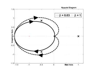
(a) Nyquist plots of the LTF of a TR repressor module which satisfies Assumption 2 for two different sets of parameters: $\beta=\bar{\beta}=10^{-1.5}$ (solid) and $\beta=\bar{\beta}=1$ (dashed). The remaining parameters are the same for both plots: $Ptot=1$, $K=100$, $\gamma=1$, $q=2$, $\alpha=100$. The points $e^{j\frac{2\pi\ell}{3}}$, $j\in\{1,2,3\}$ that appear in the criterion (9) are marked with “X”. For the solid Nyquist plot, there are no clockwise encirclements of these three points so we have BIBO stability for the feedback LTF, whereas for the dashed Nyquist plot this is not the case.

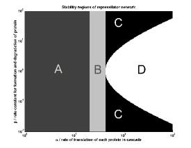
(b) Stability regions for the 3-gene Repressilator, as a function of the parameters $\alpha$ and $\beta=\bar{\beta}$, under Assumption 2. The (sufficient) condition (12) allows us to conclude that the equilibrium is GAS in region “A;” the (sufficient) condition (C.3) allows us to conclude that the equilibrium is LAS in regions “A” and “B;” and the (necessary and sufficient) condition (9) allows us to conclude that the equilibrium is LAS in regions “A,” “B” and “C;” and also that it is unstable in region “D.” The Repressilator oscillates in region “D”, assuming that there are no repeated poles. [41].

Figure 16: Nyquist plots and simulation results

An alternative approach that can be used to determine convergence to the equilibrium of a negative feedback interconnection is based on the Secant Criterion [42, 43] and some of its more recent variations [21], which apply to systems of the form

$$[\dot{\bar{\mathcal{S}}}_{i}] =u_{i}-c_{i}([\bar{\mathcal{S}}_{i}]), y_{i} =d_{i}([\bar{\mathcal{S}}_{i}]), i\in\{1,2,\dots,M\},$$ (10)

with all the $d_{i}(\cdot)$ monotone strictly increasing, connected in feedback according to

$$u_{1} =y_{M}, u_{i} =y_{i-1},\quad i\in\{2,3,\dots,M\}.$$

When an odd number of the functions $c_{i}(.)$ are monotone strictly decreasing and the remaining $c_{i}(\cdot)$ are monotone strictly increasing, the unique equilibrium point of the resulting negative feedback interconnection is LAS if

$$\prod_{i=1}^{M}\bigg{|}\frac{\frac{\partial d_{i}(s_{i})}{\partial s_{i}}\big{|}_{s_{i}=[\bar{\mathcal{S}}_{i}]^{*}}}{\frac{\partial c_{i}(s_{i})}{\partial s_{i}}\big{|}_{s_{i}=[\bar{\mathcal{S}}_{i}]^{*}}}\bigg{|}<\sec\left({\frac{\pi}{M}}\right)^{M}$$ (11)

where the $[\bar{\mathcal{S}}_{i}]^{*}$ denote the concentration of the species $\bar{\mathcal{S}}_{i}$ at the equilibrium. Equation (C.3) is a sufficient but not necessary condition for local asymptotic stability, which means that the equilibrium could still be LAS if this condition fails, as opposed to (9) which is a necessary and sufficient condition.

The secant-like criterion adapted from [21] provides the following sufficient (but typically not necessary) condition for the equilibrium point to be globally asymptotically stable (GAS): There exist constants $\phi_{i}$, $i\in\{1,2,\dots,M\}$, such that

$$\prod_{i=1}^{M}\phi_{i} <\sec\left({\frac{\pi}{M}}\right)^{M}, \Big{|}\frac{\partial d_{i}(s_{i})}{\partial s_{i}}\Big{|} \leq\phi_{i}\frac{\partial c_{i}(s_{i})}{\partial s_{i}},\quad\forall s_{i}\neq\left[\bar{\mathcal{S}}_{i}\right]^{*},\;i\in\{1,2,\dots,M\}.$$ (12)

When the equilibrium is GAS, we can conclude that the concentration of the species converge to the unique equilibrium point, regardless of their initial concentration. For either condition, knowledge of the derivatives of the functions $c_{i}(.)$ and $d_{i}(.)$ suffices to establish local or global asymptotic stability of the equilibrium of the overall network.

Under Assumption 2, it turns out that each TR repressor module under corresponds to a couple of equations of the form (C.2), one with $c_{i}(\cdot)$ monotone strictly increasing and the other with $c_{i}(\cdot)$ monotone strictly decreasing. We can therefore use the conditions (C.3) and (12) with $M=2N$ for the analysis of the Repressilator network, and can conclude that the equilibrium point of the Repressilator is LAS when

$$\frac{2P^{\textup{tot}}\alpha\beta\frac{u^{*}}{\bar{\beta}}}{\bar{\beta}K\gamma\left(1+\frac{1}{K}(\frac{u^{*}}{\bar{\beta}})^{2}\right)^{2}}<\sec\left(\frac{\pi}{2N}\right)^{2},$$ (13)

where $u^{*}$ is the unique solution to

$$\frac{\alpha\beta P^{\mathrm{tot}}}{\gamma\Big{(}1+\frac{(\frac{u^{*}}{\bar{\beta}})^{2}}{K}\Big{)}}=u^{*},$$ (14)

and GAS when

$$\frac{3P^{\textup{tot}}\alpha\beta}{8\overline{\beta}\gamma}\sqrt{\frac{3}{K}}<\sec\left(\frac{\pi}{2N}\right)^{2}.$$ (15)

For simplicity, we assumed a Hill Coefficient $q=2$. We emphasize that all the parameters that appear in equations (C.26)–(C.28) are intrinsic to a single repressor module, showing how we can again infer stability properties of Repressilator from properties of a single TR repressor module. The details of the computations that lead to (C.26)–(C.28) can be found in Appendix C.

Figure 16(b) shows the stability regions for a 3-gene Repressilator as we vary two of the TR module parameters.

5 Conclusions and Future Work

We addressed the decomposition of biochemical networks into functional modules, focusing our efforts on demonstrating how the behavior of a complex network can be inferred from the properties of its constituent modules.

To illustrate our approach, we studied systems that have received significant attention in the systems biology literature: gene regulatory networks, enzymatic networks, and signaling pathways. Our primary goal in defining these modules was to make sure that the modules exhibited dynamic and parametric modularity, while making sure that they had a clear biological function: regulating the production of a protein, transforming a substrate into a different protein, or transmitting information within a cell.

A key issue that has not been addressed here is how one could go about partitioning a biological network whose function is not known a priori, into a set of biologically “meaningful” modules. In the terminology of Section 2, this question could be stated as how to determine a partition for the dynamic DBSR graph that leads to biologically “meaningful” modules — recall that this section provides a procedure to define the modules, assuming that a partition of the dynamic DBSR graph has been given. We conjecture that biologically meaningful partitions can be obtained by minimizing the number of signals needed to interconnect the modules, which corresponds to minimizing the number of arrows in the dynamic DBSR graph that need to be “severed” by the partition (cf. Rule 3). The rationale for this conjecture lies in the principle that functionally meaningful modules should be sparsely connected, processing a small number of inputs to produce a small number of outputs. In fact, most of the modules that we introduced in Section 3 have a single input and a single output, with the exception of the multi-gene TR module and the PD-cycle module that needs two inputs and two outputs for the bidirectional transmission of information in the signaling pathway.

An important question in our current research is precisely to develop methods to partition large biological networks into biologically “meaningful” modules, using methods similar to those introduced in [32, 31]. This could allow us to “discover” biological function in these networks.

APPENDIX

Appendix A Module Characteristics

In this section, we present some properties of the modules that could not be fit into the main paper.

Transcriptional regulation (TR) module

In Table 1 of the main paper, we presented the LTF of a TR module when Assumptions 1–2 were satisfied. A comprehensive explanation of how the dynamics of a TR module are simplified with Assumption 2 is provided in [14].

It is reasonably straightforward to compute the LTF of a TR module when only Assumption 1 is satisfied, and it is given by

$$H_{j}(s)=D_{j}\frac{qk^{\textup{on}}\frac{KP^{\textup{tot}}(\theta u^{*})^{q}}{K+(\theta u^{*})^{q}}\alpha_{j}\beta_{j}}{\Big{(}\theta u^{*}(s+k^{\textup{off}})(s+\bar{\beta})+k^{\textup{on}}(\theta u^{*})^{q}\big{(}(q^{2}F\frac{KP^{\textup{tot}}(\theta u^{*})^{q}}{K+(\theta u^{*})^{q}}+\theta u^{*})s+u^{*}\big{)}\Big{)}(s+\gamma_{j})}$$

with

$$D_{j} \coloneq\begin{cases}+1&\text{if $\mathcal{S}_{0}$ activates $\mathcal{G}_{j}$}\\ -1&\text{if $\mathcal{S}_{0}$ represses $\mathcal{G}_{j}$},\end{cases}\qquad\theta\coloneq\frac{1}{\bar{\beta}}.$$

This LTF now depends on the fan-out $F$. It is worth noting that the LTFs to each activating and to each repressing output are exactly the same because of Assumption 1. If this were not the case, the same method could be utilized to compute the LTF, but the expression would look different for each output. [44] contains more information on how to compute the LTF of the module given the ODEs.

Enzyme-substrate reaction (ESR) module

The properties of ESR modules are summarized in Table 2 of the main paper. The characteristics of these modules have been presented using two classical approximations to simplify the reaction dynamics.

The form of the LTF obtained when using the quasi steady-state approximation (Assumption 4 from the main paper) was compact enough to fit in the main paper, but not the LTF when using the equilibrium approximation (Assumption 3 from the main paper). Under Assumption 3, the LTF of an ESR module is given by

$$\frac{K^{\mathrm{p}}(u^{*})}{s+K^{\mathrm{q}}(u^{*})}$$

where

$$K^{\mathrm{p}}(u^{*}) =\frac{E^{\textup{tot}}k^{\textup{cat}}K^{\mathrm{d}}}{(K^{\mathrm{d}}+\left[\mathcal{S}_{0}\right]^{*})^{2}}$$

$$K^{\mathrm{q}}(u^{*}) =\frac{N}{\left(E^{\textup{tot}}K^{\mathrm{d}}+(K^{\mathrm{d}}+\left[\mathcal{S}_{0}\right]^{*})^{2}\right)^{2}}$$

with

$$N =E^{\textup{tot}}K^{\mathrm{d}}\Big{(}(K^{\mathrm{d}}+\left[\mathcal{S}_{0}\right]^{*})\big{(}k^{\textup{cat}}(K^{\mathrm{d}}+\left[\mathcal{S}_{0}\right]^{*})+$$

$$\qquad\gamma(K^{\mathrm{d}}+3\left[\mathcal{S}_{0}\right]^{*})-2u^{*}\big{)}+k^{\textup{cat}}E^{\textup{tot}}(K^{\mathrm{d}}+2\left[\mathcal{S}_{0}\right]^{*})\Big{)}+\gamma(K^{\mathrm{d}}+\left[\mathcal{S}_{0}\right]^{*})^{4}$$

and

$$\left[\mathcal{S}_{0}\right]^{*} =\frac{-E^{\textup{tot}}k^{\textup{cat}}+u^{*}-\gamma K^{\mathrm{d}}+\sqrt{(-E^{\textup{tot}}k^{\textup{cat}}+u^{*}-\gamma K^{\mathrm{d}})^{2}+4u^{*}\gamma K^{\mathrm{d}}}}{2\gamma}.$$

PD-cycle module

The PD-cycle module was discussed in detail in Section 3.4 of the main paper, but the LTF was omitted due to lack of space and is shown in this section.

The equilibrium point of the module as a function of the constant inputs $v_{i}^{*}$, $u_{i}^{*}$ are given by

$$\left[\mathcal{S}_{i+1}\right]^{*} =\frac{\bar{k}^{\mathrm{f}}_{i}(k^{\textup{r}}_{i}+\alpha_{i})v_{i}^{*}(E^{\textup{tot}}_{i}\bar{\alpha}_{i}-u_{i}^{*})}{k^{\textup{f}}_{i}\alpha_{i}(\bar{k}^{\mathrm{r}}_{i}+\bar{\alpha}_{i})u_{i}^{*}}, [\mathcal{S}_{i}^{\dagger}\textup{:}\mathcal{S}_{i+1}]^{*} =\frac{v_{i}^{*}}{\alpha_{i}}$$

$$[\mathcal{S}_{i}^{\dagger}]^{*} =\frac{u_{i}^{*}(\bar{k}^{\mathrm{r}}_{i}+\bar{\alpha}_{i})}{\bar{k}^{\mathrm{f}}_{i}(E^{\textup{tot}}_{i}\bar{\alpha}_{i}-u_{i}^{*})}, \left[E_{i}\right]^{*} =E^{\textup{tot}}_{i}-\frac{u_{i}^{*}}{\bar{\alpha}_{i}}$$

and the LTF around this equilibrium is given by

$$H(s)\coloneq\frac{1}{D(s)}\begin{bmatrix}N_{11}(s)&N_{12}(s)\\ N_{21}(s)&N_{22}(s)\end{bmatrix}$$

where

$$N_{11}(s) ={k^{\textup{f}}_{i}}{[\mathcal{S}_{i}^{\dagger}]^{*}}({\left[E_{i}\right]^{*}}{\bar{k}^{\mathrm{f}}_{i}}(s+{\bar{\alpha}_{i}})+s({\bar{k}^{\mathrm{r}}_{i}}+s+{\bar{k}^{\mathrm{f}}_{i}}{[\mathcal{S}_{i}^{\dagger}]^{*}}+{\bar{\alpha}_{i}})){\alpha_{i}}$$

$$N_{12}(s) ={k^{\textup{f}}_{i}}s{\left[\mathcal{S}_{i+1}\right]^{*}}({\bar{k}^{\mathrm{r}}_{i}}+s+{\bar{k}^{\mathrm{f}}_{i}}{[\mathcal{S}_{i}^{\dagger}]^{*}}+{\bar{\alpha}_{i}}){\alpha_{i}}$$

$$N_{21}(s) =-{\left[E_{i}\right]^{*}}{\bar{k}^{\mathrm{f}}_{i}}{k^{\textup{f}}_{i}}s{[\mathcal{S}_{i}^{\dagger}]^{*}}{\bar{\alpha}_{i}}$$

$$N_{22}(s) ={\left[E_{i}\right]^{*}}{\bar{k}^{\mathrm{f}}_{i}}{\bar{\alpha}_{i}}({k^{\textup{r}}_{i}}s+(s+{k^{\textup{f}}_{i}}{[\mathcal{S}_{i}^{\dagger}]^{*}})(s+{\alpha_{i}})),$$

$$D(s) =\left[E_{i}\right]^{*}\bar{k}^{\mathrm{f}}_{i}(s+\bar{\alpha}_{i})\big{(}k^{\textup{r}}_{i}s+(s+k^{\textup{f}}_{i}\left[\mathcal{S}_{i}\right]^{*})(s+\alpha_{i})\big{)}+$$

$$\quad s\big{(}s+\bar{k}^{\mathrm{r}}_{i}+\bar{k}^{\mathrm{f}}_{i}\left[\mathcal{S}_{i}\right]^{*}+\bar{\alpha}_{i}\big{)}\big{(}s^{2}+(k^{\textup{r}}_{i}+k^{\textup{f}}_{i}([\mathcal{S}_{i}^{\dagger}\textup{:}\mathcal{S}_{i+1}]^{*}+\left[\mathcal{S}_{i}\right]^{*})+\alpha_{i})s+\alpha_{i}k^{\textup{f}}_{i}\left[\mathcal{S}_{i}\right]^{*}\big{)}.$$

Appendix B Covalent Modification Network

To prove the statements from the main paper about the Covalent Modification network, we use the following result which is adapted from [20, Theorems 2-3], and provides conditions that can be used to establish the stability of the equilibrium points for positive feedback networks. To express the result, we need the following definitions which are closely related to that of cooperativity: We say that the system

$$\dot{x} =A(x,u), y =B(x), x\in\mathbb{R}^{n},u\in\mathbb{R}^{k},y\in\mathbb{R}^{m},$$ (B.1)

is excitable (with respect to the positive orthant) if for every initial condition $x_{0}\in\mathbb{R}^{n}$ and all inputs $u(t),\bar{u}(t)\in\mathbb{R}^{k}$, $\forall t\geq 0$, we have that

$$u(t)\succ\bar{u}(t),\;\forall t\geq 0\quad\Rightarrow\quad x(t;x_{0},u)\gg x(t;x_{0},\bar{u}),\;\forall t>0,$$

and it is transparent (with respect to the positive orthant) if for all initial conditions $x_{0},\bar{x}_{0}\in\mathbb{R}^{n}$ and every input $u(t)\in\mathbb{R}^{k}$, $\forall t\geq 0$, we have that

$$x_{0}\succ\bar{x}_{0}\quad\Rightarrow\quad x(t;x_{0},u)\gg x(t;\bar{x}_{0},u),\;\forall t>0.$$

Given two vectors $v,\bar{v}$, we write $v\succ\bar{v}$ if every entry of $v$ is larger than or equal to the corresponding entry of $\bar{v}$ and $v\neq\bar{v}$.

Theorem 1

Consider the feedback interconnection depicted in Figure 12(a) with $u(t)=0$, $\forall t\geq 0$ and $\mathcal{M}_{1}$ SISO of the form (B.1). Assume that

1. $\mathcal{M}_{1}$ is excitable, transparent, and cooperative with a well-defined ISSCF and IOSCF;

2. for every constant input $u_{1}(t)=u_{1}^{*}$, $\forall t\geq 0$ to $\mathcal{M}_{1}$, the Jacobian matrix $\frac{\partial A(x,u_{1})}{\partial x}$ is nonsingular at the corresponding equilibrium, which is globally asymptotically stable;

3. the IOSCF $f_{1}(u_{1}^{*})$ of $\mathcal{M}_{1}$ has fixed points $u^{*}$ for which $f_{1}(u^{*})=u^{*}$ and $\frac{\partial f_{1}(u_{1}^{*})}{\partial u_{1}^{*}}\Big{|}_{u_{1}^{*}=u^{*}}\neq 1$;

4. all trajectories of the feedback interconnection are bounded.

Then, for almost all initial conditions, the solutions converge to the set of points for which $f_{1}(u_{1}^{*})=u_{1}^{*}$ and $\frac{\partial f_{1}(u_{1}^{*})}{\partial u_{1}^{*}}~{}<~{}1$. $\Box$

We now use Theorem 1 to prove Corollary 1.

Corollary 1

Consider the covalent modificiation network shown in Figure 14, which consists of a cascade of two ESR modules connected in positive feedback. The substrate concentrations in each module converges to $0$ as $t\to\infty$.  $\Box$

• We consider the covalent modificiation network adapted from [26], which is a network given by the chemical reactions

  $$\begin{split}\mathcal{S}_{1}+E_{1}\xrightleftharpoons[k^{\textup{r}}_{1}\left[\mathcal{S}_{1}\textup{:}E_{1}\right]]{k^{\textup{f}}_{1}\left[\mathcal{S}_{1}\right]\left[E_{1}\right]}\mathcal{S}_{1}\textup{:}E_{1}&\xrightarrow{k^{\textup{cat}}_{1}\left[\mathcal{S}_{1}\textup{:}E_{1}\right]}\mathcal{S}_{2}+E_{1}\\ \mathcal{S}_{2}+E_{2}\xrightleftharpoons[k^{\textup{r}}_{2}\left[\mathcal{S}_{2}\textup{:}E_{2}\right]]{k^{\textup{f}}_{2}\left[\mathcal{S}_{2}\right]\left[E_{2}\right]}\mathcal{S}_{2}\textup{:}E_{2}&\xrightarrow{k^{\textup{cat}}_{2}\left[\mathcal{S}_{2}\textup{:}E_{2}\right]}\mathcal{S}_{1}+E_{2}\\ \mathcal{S}_{1}&\xrightarrow{\gamma_{1}\left[\mathcal{S}_{1}\right]}\varnothing\\ \mathcal{S}_{2}&\xrightarrow{\gamma_{2}\left[\mathcal{S}_{2}\right]}\varnothing.\end{split}$$ (B.2)

  This network can be viewed as a positive feedback interconnection of a cascade of two ESR modules described in Table 2 of the main paper, one containing the substrate $\mathcal{S}_{1}$ and the other the substrate $\mathcal{S}_{2}$. We call these modules $\mathcal{M}_{1}$ and $\mathcal{M}_{2}$, and the module dynamics for $i=\{1,2\}$ are each given by

  $$\bm{\mathcal{M}_{i}}:\dot{\left[\mathcal{S}_{i}\right]} =A_{i}(\left[\mathcal{S}_{i}\right],u_{i}), y_{i} =B_{i}(\left[\mathcal{S}_{i}\right])$$

  where

  $$A_{i}(\left[\mathcal{S}_{i}\right],u_{i}) =\frac{u_{i}-\gamma_{i}\left[\mathcal{S}_{i}\right]-\frac{k^{\textup{cat}}_{i}E^{\textup{tot}}_{i}\left[\mathcal{S}_{i}\right]}{K^{\mathrm{d}}_{i}+\left[\mathcal{S}_{i}\right]}}{1+\frac{K^{\mathrm{d}}_{i}E^{\textup{tot}}_{i}}{(K^{\mathrm{d}}_{i}+\left[\mathcal{S}_{i}\right]^{2})}} B_{i}(\left[\mathcal{S}_{i}\right]) =\frac{k^{\mathrm{cat}}E^{\textup{tot}}_{i}\left[\mathcal{S}_{i}\right]}{K^{\mathrm{d}}_{i}+\left[\mathcal{S}_{i}\right]}$$ (B.3)

  under Assumption 3, and

  $$A_{i}(\left[\mathcal{S}_{i}\right],u_{i}) =u_{i}-\gamma_{i}\left[\mathcal{S}_{i}\right]-\frac{k^{\mathrm{cat}}_{i}E^{\textup{tot}}_{i}\left[\mathcal{S}_{i}\right]}{K^{\mathrm{m}}_{i}+\left[\mathcal{S}_{i}\right]} B_{i}(\left[\mathcal{S}_{i}\right]) =\frac{k^{\mathrm{cat}}_{i}E^{\textup{tot}}_{i}\left[\mathcal{S}_{i}\right]}{K^{\mathrm{m}}_{i}+\left[\mathcal{S}_{i}\right]}$$ (B.4)

  under Assumption 4. The covalent modification system consists of the modules $\mathcal{M}_{1}$ and $\mathcal{M}_{2}$ interconnected with $y_{1}=u_{2}$ and $y_{2}=u_{1}$.

We first need to show that the cascade of two ESR modules satisfies the properties in item 1 from Theorem 1. For the cascade network with $y_{1}=u_{2}$ and the module dynamics (B.3) or (B.4), we have

$$\frac{\partial A_{1}(\left[\mathcal{S}_{1}\right],u_{1})}{\partial u_{1}}=1 \qquad\frac{\partial A_{2}(\left[\mathcal{S}_{2}\right],u_{2})}{\partial\left[\mathcal{S}_{1}\right]}>0\qquad\frac{\partial y_{2}}{\partial\left[\mathcal{S}_{2}\right]}>0$$

$$\frac{\partial A_{1}(\left[\mathcal{S}_{1}\right],u_{1})}{\partial\left[\mathcal{S}_{2}\right]}=0 \qquad\frac{\partial A_{2}(\left[\mathcal{S}_{2}\right],u_{2})}{\partial u_{1}}=0\qquad\frac{\partial y_{2}}{\partial\left[\mathcal{S}_{1}\right]}=0,$$

from which we can infer several properties: From [19, Propositon 1], we conclude that the cascade is cooperative, from [20, Theorem 4] that it is excitable, and from [20, Theorem 5] that it is transparent. For simplicity, in the rest of the proof we use Assumption 3 and therefore the module dynamics in (B.3), but the proof would be similar for the module dynamics in (B.4).

The IOSCF of the cascade is well-defined and given by $f_{2}(f_{1}(u_{1}^{*}))$, where $u_{1}^{*}$ denotes a constant input to the cascade and

$$f_{i}(u_{i}^{*}) \coloneq y_{i}^{*}=\frac{1}{2}(u_{i}^{*}+k^{\mathrm{cat}}_{i}E^{\textup{tot}}_{i}+K^{\mathrm{d}}_{i}\gamma_{i}-\sqrt{(-u_{i}^{*}+k^{\mathrm{cat}}_{i}E^{\textup{tot}}_{i}+K^{\mathrm{d}}_{i}\gamma_{i})^{2}+4K^{\mathrm{d}}_{i}u_{i}^{*}\gamma_{i}})\qquad i=\{1,2\}.$$

The ISSCF of the cascade is also well-defined, with the equilibrium states corresponding to a constant input $u_{1}^{*}$ to the cascade given by

$$\left[\mathcal{S}_{1}\right]^{*}=g_{1}(u_{1}^{*}),\quad\left[\mathcal{S}_{2}\right]^{*}=g_{2}(g_{1}(u_{1}^{*}))$$

where

$$g_{i}(u_{i}^{*}) =\frac{1}{2}(K^{\mathrm{p}}_{i}+\sqrt{4K^{\mathrm{d}}_{i}\gamma_{i}u_{i}^{*}+(K^{\mathrm{p}}_{i})^{2}}) K^{\mathrm{p}}_{i} \coloneq u_{i}^{*}-K^{\mathrm{d}}_{i}\gamma_{i}-k^{\mathrm{cat}}_{i}E^{\textup{tot}}_{i}, i\in\{1,2\}.$$

Therefore the cascade of two ESR modules satisfies the properties in item 1 of Theorem 1.

We now show that the cascade of two ESR modules satisfies the properties in item 2 from Theorem 1. For some constant input $u_{1}^{*}\geq 0$, the Jacobian matrix of the interconnection is given by the $2\times 2$ lower triangular matrix

$$J=\begin{bmatrix}J_{11}&0\\ J_{21}&J_{22},\end{bmatrix}$$

which is non-singular because $J_{11}>0$ and $J_{22}>0$, under the implicit assumption that all parameters within each module are positive.

Each of the modules $\mathcal{M}_{1}$ and $\mathcal{M}_{2}$ has an equilibrium point that is globally asymptotically stable for some constant input $u_{i}^{*}$ into each module. This can be verified by doing the coordinate transformation $x_{i}=\left[\mathcal{S}_{i}\right]-\left[\mathcal{S}_{i}\right]^{*}$ and observing that the Lyapunov function $V(x_{i})=x_{i}^{2}$ is zero-at-zero, locally positive definite and $\dot{V}(x_{i})<0$, $\forall x_{i}$, $i\in\{1,2\}$. The cascade of both the modules also has a globally asymptotically stable equilibrium point, as can be seen from the argument in [45].

To verify that the cascade of the ESR modules satisfies the property in item 3 from Theorem 1, we will show that $f_{2}(f_{1}(u_{1}^{*}))=u_{1}^{*}$ has a unique solution at $u_{1}^{*}=0$, and also that

$$\frac{\partial f_{2}(f_{1}(u_{1}^{*}))}{\partial u_{1}^{*}}\Bigg{|}_{u_{1}^{*}=0}<1.$$

To show that $f_{2}(f_{1}(u_{1}^{*}))=u_{1}^{*}$ has a unique solution at $u_{1}^{*}=0$, we first observe that the IOSCFs of $\mathcal{M}_{1}$ and $\mathcal{M}_{2}$ are each monotone increasing and strictly concave, since $f_{i}^{\prime}(u_{i}^{*})>0$ and $f_{i}^{\prime\prime}(u_{i}^{*})<0$, $\forall i\in\{1,2\}$. Then from

$$\frac{\partial f_{2}\left(f_{1}\left(u_{1}^{*}\right)\right)}{\partial u_{1}^{*}} =f_{1}^{\prime}(u_{1}^{*})f_{2}^{\prime}\left(f_{1}\left(u_{1}^{*}\right)\right)$$ (B.5)

$$\frac{\partial^{2}f_{2}\left(f_{1}\left(u_{1}^{*}\right)\right)}{\partial(u_{1}^{*})^{2}} =f_{1}^{\prime\prime}(u_{1}^{*})f_{2}^{\prime}\left(f_{1}\left(u_{1}^{*}\right)\right)+\left(f_{1}^{\prime}\left(u_{1}^{*}\right)\right)^{2}f_{2}^{\prime\prime}\left(f_{1}\left(u_{1}^{*}\right)\right),$$ (B.6)

it can be seen that the cascade of $\mathcal{M}_{1}$ and $\mathcal{M}_{2}$ is also monotone increasing and strictly concave because

1. $f_{1}^{\prime}(u_{1}^{*})>0$ and $f_{2}^{\prime}(u_{2}^{*})>0\quad\forall u_{1}^{*},u_{2}^{*}>0\implies\frac{\partial f_{2}\left(f_{1}\left(u_{1}^{*}\right)\right)}{\partial u_{1}^{*}}>0$ from (B.5).

2. $f_{1}^{\prime\prime}(u_{1}^{*})<0$ and $f_{2}^{\prime\prime}(u_{2}^{*})<0\quad\forall u_{1}^{*},u_{2}^{*}>0\implies\frac{\partial^{2}f_{2}\left(f_{1}\left(u_{1}^{*}\right)\right)}{\partial(u_{1}^{*})^{2}}<0$ from (B.6).

Therefore, there can be no other solution to $f_{2}(f_{1}(u_{1}^{*}))=u_{1}^{*}$ other than $u_{1}^{*}=0$. In addition, the IOSCF of the cascade is given by

$$\frac{\partial f_{2}(f_{1}(u_{1}^{*}))}{\partial u_{1}^{*}}\Big{|}_{u_{1}^{*}=0}=\frac{E^{\textup{tot}}_{1}E^{\textup{tot}}_{2}k^{\textup{cat}}_{1}k^{\textup{cat}}_{2}}{(E^{\textup{tot}}_{1}k^{\textup{cat}}_{1}+K^{d}_{1}\gamma_{1})(E^{\textup{tot}}_{2}k^{\textup{cat}}_{2}+K^{d}_{2}\gamma_{2})},$$

which is always less than $1$ since all parameters are positive by definition.

The boundedness property in item 4 of Theorem 1 follows from techniques used to analyze MAK ODEs from [46, Main Technical Lemma], which can be applied to the covalent modificiation network.

Appendix C Repressilator network

Generalized Nyquist Criterion

We first present a result that will be used to prove Corollary 2. The following result is inspired by the Nyquist Stability Criterion [40] and provides a necessary and sufficient condition to establish the BIBO stability of the LTF of a feedback interconnection of a cascade of $N\geq 1$ modules, each with an equal LTF as depicted in Figure C.1.

Theorem 2

Consider the feedback interconnection of a cascade of $N$ modules depicted in Figure C.1, all with the same LTF $H_{1}(s)$ around a given equilibrium point of the feedback interconnection. Then the LTF of the feedback connection is BIBO stable if and only if

$$\#OUP=-\frac{1}{N}\sum_{\ell=1}^{N}\#END[e^{j\frac{2\pi\ell}{N}}],$$

where $\#OUP$ represents the number of (open-loop) unstable poles of $H_{1}(s)$ and $\#END[e^{j\frac{2\pi\ell}{N}}]$ denotes the number of clockwise encirclements of the Nyquist contour of $H_{1}(j\omega)$, $\omega\in\mathbb{R}$ around the point $e^{j\frac{2\pi\ell}{N}}$ on the complex plane. $\Box$

Figure C.1: Cascade of $N$ modules, each with an equal LTF $H_{1}(s)$, connected in feedback. Theorem 2 provides conditions for the BIBO stability of the linearized network, from a small perturbation in $u$ to a small perturbation in $y$.

• To investigate the BIBO stability of the LTF of the network in Figure C.1, we consider the characteristic equation of the feedback loop: $1-H_{1}(s)^{N}=0$. The number of unstable poles is thus given by the unstable solutions to the equation:

  $$1-H_{1}(s)^{N}=0\quad\Leftrightarrow\quad\exists i\in\{1,2,\cdots,n\},\;H_{1}(s)=z_{i},$$

  where $z_{\ell}\coloneq e^{j\frac{2\pi\ell}{N}}$ are the $N$ roots to the equation $z^{N}=1$.

To count the number of unstable poles of the network, we must then add the number of unstable poles of each of the $N$ equations

$$H_{1}(s)=z_{\ell},\quad\ell\in\{1,2,\cdots,N\},$$

which can be done using Cauchy’s argument principle by counting the number of clockwise encirclements of the point $z_{\ell}\in\mathbb{C}$ for the Nyquist contour of $H_{1}(j\omega)$, $\omega\in\mathbb{R}$.   

Corollary 2

Consider a Repressilator network, that consists of an odd number $N$ of equal single-gene TR repressor modules ($F=1$) connected in feedback as in Figure 15(b). The network has a unique equilibrium point that is locally asymptotically stable if and only if

$$\sum_{\ell=1}^{N}\#END[e^{j\frac{2\pi\ell}{N}}]=0,$$

where $\#END[e^{j\frac{2\pi\ell}{N}}]$ denotes the number of clockwise encirclements of the Nyquist plot of the LTF of a single TR repressor module around the point $e^{j\frac{2\pi\ell}{N}}$.  $\Box$

• We assume that Assumption 2 is satisfied for simplicity, although it is straightforward to extend the proof for the case when it is not. Corollary 2 follows from Theorem 2 by recognizing that a single-gene repressor TR module can be represented by the following LTF

  $$H_{1}(s) =-\frac{qKP^{\mathrm{tot}}\alpha_{1}\beta_{1}(\frac{u^{*}}{\bar{\beta}})^{q-1}}{(K+(\frac{u^{*}}{\bar{\beta}})^{q})^{2}(s+\gamma_{1})(s+\bar{\beta})}$$ (C.1)

  under Assumption 2. Moreover, since the network input $u(t)=0$ $\forall t\geq 0$ and all modules have identical parameters, the values of the inputs and outputs of each module at equilibrium will be the same, each given by the unique solution $u^{*}$ to (C.27). Therefore all modules have equal LTFs, and this enables us to use Theorem 2 to analyze when the LTF of the Repressilator is BIBO stable.

To complete the proof, we need to show that if the LTF of the Repressilator network is BIBO stable, then the equilibrium point is locally asymptotically stable. To do this, we need to show that the realization of the linearized network is minimal [34]. Defining the state of the network to be

$$x=\begin{bmatrix}\left[\mathcal{S}_{1}\right]\\ \left[mRNA_{1}\right]\\ \left[\mathcal{S}_{2}\right]\\ \left[mRNA_{2}\right]\\ \vdots\\ \vdots\\ \left[\mathcal{S}_{N}\right]\\ \left[mRNA_{N}\right]\end{bmatrix},$$

the state-space realization of the linearized closed-loop Repressilator network is given by

$$\dot{\delta x}=A\delta x+B\delta u\qquad\delta y=C\delta x$$

where

$$A_{2N\times 2N} =\setcounter{MaxMatrixCols}{11}\begin{bmatrix}-\bar{\beta}&0&0&0&0&\cdots&0&0&0&0&\beta\\ P&-\gamma&0&0&0&\cdots&0&0&0&0&0\\ 0&\beta&-\bar{\beta}&0&0&\cdots&0&0&0&0&0\\ 0&0&P&-\gamma&0&\cdots&0&0&0&0&0\\ \vdots&\vdots&\vdots&\vdots&\vdots&\ddots&\vdots&\vdots&\vdots&\vdots&\vdots\\ \vdots&\vdots&\vdots&\vdots&\vdots&&\ddots&\vdots&\vdots&\vdots&\vdots\\ 0&0&0&0&0&\cdots&\beta&-\bar{\beta}&0&0&0\\ 0&0&0&0&0&\cdots&0&P&-\gamma&0&0\\ 0&0&0&0&0&\cdots&0&0&\beta&-\bar{\beta}&0\\ 0&0&0&0&0&\cdots&0&0&0&P&-\gamma\end{bmatrix}$$

$$B_{2N\times 1} =\begin{bmatrix}1\\ 0\\ \vdots\\ 0\\ 0\end{bmatrix}\qquad C_{1\times 2N}=\begin{bmatrix}0&0&\cdots&0&\bar{\beta}\end{bmatrix}\qquad P=-\frac{q\alpha P^{\textup{tot}}K(\left[\mathcal{S}_{i}\right]^{*})^{q-1}}{(K+(\left[\mathcal{S}_{i}\right]^{*})^{q})^{2}}\quad\forall i.$$

Both the controllability and observability matrices of this system have full rank and therefore the realization is minimal [34]. In this case, BIBO stability of the LTF implies that the realization is exponentially stable and therefore the equilibrium is locally asymptotically stable.  $\Box$

Figure 16(a) shows a numerical example of the Nyquist plot of (C.1) when $N=3$. When Assumption 2 is not satisfied, (C.1) is given by the more complicated LTF that is presented in Appendix A.

Generalized Secant Criterion

The following result provides a alternative condition that can be used to establish the stability of a negative feedback interconnection of a cascade of $N$ modules, not necessarily with the same LTFs. This result will be used to prove Corollary 3, but can be used for a wide variety of networks. This new condition is inspired by results in [42, 43, 21] and applies to the feedback interconnection depicted in Figure 15(b), where the modules $\mathcal{M}_{i}$ are each described by equations of the following form

$$\dot{\left[\mathcal{S}_{i}\right]} =u_{i}-c_{i}(\left[\mathcal{S}_{i}\right]), y_{i} =d_{i}(\left[\mathcal{S}_{i}\right]), i\in\{1,2,\dots,N\},$$ (C.2)

for appropriate scalar functions $c_{i}(\cdot)$, $d_{i}(\cdot)$. All the functions $c_{i}(\cdot)$ are assumed to be monotone strictly increasing and the functions $d_{i}(.)$ are assumed to be either monotone strictly decreasing or strictly increasing. The IOSCF of the $i$th module is given by

$$f_{i}(u_{i}^{*})=d_{i}\big{(}c_{i}^{-1}(u_{i}^{*})\big{)},\quad\forall u_{i}^{*}\in\mathbb{R},$$

where $c_{i}^{-1}(\cdot)$ denotes the inverse function of $c_{i}(\cdot)$, which is invertible and monotone strictly increasing since $c_{i}(\cdot)$ is monotone strictly increasing. Therefore, $f_{i}(u_{i}^{*})$ has the same (strict) monotonicity as $d_{i}(\cdot)$. The result that follows considers the case in which we have an odd number of $d_{i}(\cdot)$ that are monotone strictly decreasing and the remaining are monotone strictly increasing. In this case, the composition of the IOSCFs of the $N$ modules is monotone strictly decreasing and we have a negative feedback interconnection.

Theorem 3

Consider the feedback interconnection depicted in Figure 15(b), with each of the $N$ modules $\mathcal{M}_{i}$ of the form (C.2), where

1. the $c_{i}(\cdot)$ are continuous and monotone strictly increasing;

2. an odd number $M\leq N$ of the $d_{i}(\cdot)$ are continuous and monotone strictly decreasing, while the remaining $N-M$ of the $d_{i}(\cdot)$ are continuous and monotone strictly increasing.

Then the IOSCF of the cascade is monotone strictly decreasing and the feedback interconnection has a unique equilibrium. This equilibrium is locally asymptotically stable provided that

$$\prod_{i=1}^{N}\bigg{|}\frac{\frac{\partial d_{i}(s_{i})}{\partial s_{i}}\big{|}_{s_{i}=\left[\mathcal{S}_{i}\right]^{*}}}{\frac{\partial c_{i}(s_{i})}{\partial s_{i}}\big{|}_{s_{i}=\left[\mathcal{S}_{i}\right]^{*}}}\bigg{|}<\sec\left({\frac{\pi}{N}}\right)^{N},$$ (C.3)

where $\left[\mathcal{S}_{i}\right]^{*}$ denotes the value of $\left[\mathcal{S}_{i}\right]$ at the equilibrium; and it is globally asymptotically stable if there exist constants $\phi_{i}>0$, $i\in\{1,2,\dots,N\}$ for which

$$\Big{|}\frac{d_{i}(z_{i})-d_{i}(\left[\mathcal{S}_{i}\right]^{*})}{c_{i}(z_{i})-c_{i}(\left[\mathcal{S}_{i}\right]^{*})}\Big{|}\leq\phi_{i}\quad\forall z_{i}\neq\left[\mathcal{S}_{i}\right]^{*}$$

and

$$\prod_{i=1}^{N}\phi_{i} <\sec\left({\frac{\pi}{N}}\right)^{N}. \Box$$  

An alternative condition to (C.17) which is simpler to verify is given by

$$\Big{|}\frac{\partial d_{i}(z_{i})}{\partial z_{i}}\Big{|}\leq\phi_{i}\frac{\partial c_{i}(z_{i})}{\partial z_{i}},\quad\forall z_{i}\neq\left[\mathcal{S}_{i}\right]^{*}.$$

• The proof of this result relies on making a coordinate transformation to our original system to take it into a form that allows us to use the secant criterion [42, 43, 21] and results in [21].

The dynamics of the feedback interconnection under consideration can be written as

$$\dot{\left[\mathcal{S}_{1}\right]} =-c_{1}(\left[\mathcal{S}_{1}\right])+d_{N}(\left[\mathcal{S}_{N}\right]),$$ (C.4a)

$$\dot{\left[\mathcal{S}_{2}\right]} =-c_{2}(\left[\mathcal{S}_{2}\right])+d_{1}(\left[\mathcal{S}_{1}\right])$$ (C.4b)

$$\;\vdots$$ (C.4c)

$$\dot{\left[\mathcal{S}_{N}\right]} =-c_{N}(\left[\mathcal{S}_{N}\right])+d_{N-1}(\left[\mathcal{S}_{N-1}\right]).$$ (C.4d)

with an equilibrium state defined by concentrations $\left[\mathcal{S}_{i}\right]^{*}$ for which

$$c_{1}(\left[\mathcal{S}_{1}\right]^{*}) =d_{N}(\left[\mathcal{S}_{N}\right]^{*}),$$ (C.5a)

$$c_{2}(\left[\mathcal{S}_{2}\right]^{*}) =d_{1}(\left[\mathcal{S}_{1}\right]^{*}),$$ (C.5b)

$$\;\vdots$$ (C.5c)

$$c_{N}(\left[\mathcal{S}_{N}\right]^{*}) =d_{N-1}(\left[\mathcal{S}_{N-1}\right]^{*}).$$ (C.5d)

To verify that such an equilibrium exists and is unique, note that we have a feedback interconnection of a cascade of $N$ systems, each with an IOSCF given by

$$f_{i}(u_{i}^{*})=d_{i}\big{(}c_{i}^{-1}(u_{i}^{*})\big{)},\quad\forall u_{1}^{*}\in\mathbb{R},$$

where $c_{i}^{-1}$ denotes the inverse function of $c_{i}$, which is invertible and monotone strictly increasing since $c_{i}$ is monotone strictly increasing. Therefore, $f_{i}(u_{i}^{*})$ has the same (strict) monotonicity as $d_{i}$. Since an odd number $M$ of the $d_{i}$ are monotone strictly decreasing, an odd number of the $f_{i}$ are also monotone strictly decreasing and therefore the composition of all the $f_{i}$ is monotone strictly decreasing. This shows that we have a negative feedback interconnection and thus a unique equilibrium.

Using (C.5), we can re-write (C.4) as

$$\dot{\left[\mathcal{S}_{1}\right]} =-c_{1}(\left[\mathcal{S}_{1}\right])+c_{1}(\left[\mathcal{S}_{1}\right]^{*})+d_{N}(\left[\mathcal{S}_{N}\right])-d_{N}(\left[\mathcal{S}_{N}\right]^{*}),$$

$$\dot{\left[\mathcal{S}_{2}\right]} =-c_{2}(\left[\mathcal{S}_{2}\right])+c_{2}(\left[\mathcal{S}_{2}\right]^{*})+d_{1}(\left[\mathcal{S}_{1}\right])-d_{1}(\left[\mathcal{S}_{1}\right]^{*}),$$

$$\;\vdots$$

$$\dot{\left[\mathcal{S}_{N}\right]} =-c_{N}(\left[\mathcal{S}_{N}\right])+c_{N}(\left[\mathcal{S}_{N}\right]^{*})+d_{N-1}(\left[\mathcal{S}_{N-1}\right])-d_{N-1}(\left[\mathcal{S}_{N-1}\right]^{*}).$$

Since we have an odd number $M\geq 1$ of functions $d_{i}$ that are monotone strictly decreasing and there is perfect symmetry in the cycle (C.4), we shall assume without loss of generality that $d_{N}$ is monotone strictly decreasing; if that were not the case we could simply shift the numbering of the modules appropriately.

We consider a coordinate transformation with

$$x_{1} =\left[\mathcal{S}_{1}\right]-\left[\mathcal{S}_{1}\right]^{*}, x_{N} =\left[\mathcal{S}_{N}\right]-\left[\mathcal{S}_{N}\right]^{*},$$ (C.6)

and the remaining $x_{i}$, $i\in\{2,3,\dots,N-1\}$ either given by

$$x_{i}=\left[\mathcal{S}_{i}\right]-\left[\mathcal{S}_{i}\right]^{*}$$ (C.7)

or given by

$$x_{i}=-\left[\mathcal{S}_{i}\right]+\left[\mathcal{S}_{i}\right]^{*};$$ (C.8)

each to be determined shortly. The coordinate transformation (C.6) leads to

$$\dot{x}_{1} =-c_{1}(\left[\mathcal{S}_{1}\right])+c_{1}(\left[\mathcal{S}_{1}\right]^{*})+d_{N}(\left[\mathcal{S}_{N}\right])-d_{N}(\left[\mathcal{S}_{N}\right]^{*})$$

$$=-c_{1}(\left[\mathcal{S}_{1}\right]^{*}+x_{1})+c_{1}(\left[\mathcal{S}_{1}\right]^{*})+d_{N}(\left[\mathcal{S}_{N}\right]^{*}+x_{N})-d_{N}(\left[\mathcal{S}_{N}\right]^{*})$$

$$=-a_{1}(x_{1})-b_{N}(x_{N})$$

with

$$a_{1}(x_{1}) \coloneq c_{1}(\left[\mathcal{S}_{1}\right]^{*}+x_{1})-c_{1}(\left[\mathcal{S}_{1}\right]^{*}), b_{N}(x_{N}) \coloneq-d_{N}(\left[\mathcal{S}_{N}\right]^{*}+x_{N})+d_{N}(\left[\mathcal{S}_{N}\right]^{*}).$$

Note that because $c_{1}$ is monotone strictly increasing and $d_{N}$ is monotone strictly decreasing, we have that

$$a_{1}(x_{1})\quad\begin{cases}>0&x_{1}>0\\ =0&x_{1}=0\\ <0&x_{1}<0.\end{cases}, b_{N}(x_{N})\quad\begin{cases}>0&x_{N}>0\\ =0&x_{N}=0\\ <0&x_{N}<0.\end{cases}$$ (C.9)

For the remaining variables $x_{i}$, $i\in\{2,3,\dots,N\}$, the coordinate transformation leads to

$$\dot{x}_{i} =$$

$$\begin{cases}c_{i}(\left[\mathcal{S}_{i}\right]^{*})-c_{i}(\left[\mathcal{S}_{i}\right])+d_{i-1}(\left[\mathcal{S}_{i-1}\right])-d_{i-1}(\left[\mathcal{S}_{i-1}\right]^{*})&\text{if }x_{i}=\left[\mathcal{S}_{i}\right]-\left[\mathcal{S}_{i}\right]^{*},\>x_{i-1}=\left[\mathcal{S}_{i-1}\right]-\left[\mathcal{S}_{i-1}\right]^{*}\\ &\text{or }x_{i}=\left[\mathcal{S}_{i}\right]-\left[\mathcal{S}_{i}\right]^{*},\>x_{i-1}=\left[\mathcal{S}_{i-1}\right]^{*}-\left[\mathcal{S}_{i-1}\right]\\ c_{i}(\left[\mathcal{S}_{i}\right])-c_{i}(\left[\mathcal{S}_{i}\right]^{*})-d_{i-1}(\left[\mathcal{S}_{i-1}\right])+d_{i-1}(\left[\mathcal{S}_{i-1}\right]^{*})&\text{if }x_{i}=\left[\mathcal{S}_{i}\right]^{*}-\left[\mathcal{S}_{i}\right],\>x_{i-1}=\left[\mathcal{S}_{i-1}\right]-\left[\mathcal{S}_{i-1}\right]^{*}\\ &\text{or }x_{i}=\left[\mathcal{S}_{i}\right]^{*}-\left[\mathcal{S}_{i}\right],\>x_{i-1}=\left[\mathcal{S}_{i-1}\right]^{*}-\left[\mathcal{S}_{i-1}\right]\end{cases}$$

$$=-a_{i}(x_{i})+b_{i-1}(x_{i-1})$$

where, for every $i\in\{2,3,\dots,N\}$,

$$a_{i}(x_{i}) \coloneq\begin{cases}c_{i}(\left[\mathcal{S}_{i}\right]^{*}+x_{i})-c_{i}(\left[\mathcal{S}_{i}\right]^{*})&x_{i}=\left[\mathcal{S}_{i}\right]-\left[\mathcal{S}_{i}\right]^{*}\\ -c_{i}(\left[\mathcal{S}_{i}\right]^{*}-x_{i})+c_{i}(\left[\mathcal{S}_{i}\right]^{*})&x_{i}=\left[\mathcal{S}_{i}\right]^{*}-\left[\mathcal{S}_{i}\right]\end{cases}$$

$$b_{i-1}(x_{i-1}) \coloneq$$

$$\begin{cases}d_{i-1}(\left[\mathcal{S}_{i-1}\right]^{*}+x_{i-1})-d_{i-1}(\left[\mathcal{S}_{i-1}\right]^{*})&\text{if }x_{i}=\left[\mathcal{S}_{i}\right]-\left[\mathcal{S}_{i}\right]^{*},\;x_{i-1}=\left[\mathcal{S}_{i-1}\right]-\left[\mathcal{S}_{i-1}\right]^{*}\\ d_{i-1}(\left[\mathcal{S}_{i-1}\right]^{*}-x_{i-1})-d_{i-1}(\left[\mathcal{S}_{i-1}\right]^{*})&\text{if }x_{i}=\left[\mathcal{S}_{i}\right]-\left[\mathcal{S}_{i}\right]^{*},\;x_{i-1}=\left[\mathcal{S}_{i-1}\right]^{*}-\left[\mathcal{S}_{i-1}\right]\\ -d_{i-1}(\left[\mathcal{S}_{i-1}\right]^{*}+x_{i-1})+d_{i-1}(\left[\mathcal{S}_{i-1}\right]^{*})&\text{if }x_{i}=\left[\mathcal{S}_{i}\right]^{*}-\left[\mathcal{S}_{i}\right],\;x_{i-1}=\left[\mathcal{S}_{i-1}\right]-\left[\mathcal{S}_{i-1}\right]^{*}\\ -d_{i-1}(\left[\mathcal{S}_{i-1}\right]^{*}-x_{i-1})+d_{i-1}(\left[\mathcal{S}_{i-1}\right]^{*})&\text{if }x_{i}=\left[\mathcal{S}_{i}\right]^{*}-\left[\mathcal{S}_{i}\right],\;x_{i-1}=\left[\mathcal{S}_{i-1}\right]^{*}-\left[\mathcal{S}_{i-1}\right].\end{cases}$$

Since all the $c_{i}$ are monotone strictly increasing, we have that

$$a_{i}(x_{i})\quad\begin{cases}>0&x_{i}>0\\ =0&x_{i}=0\\ <0&x_{i}<0.\end{cases}, \forall i\in\{2,3,\dots,N\}.$$

We have already selected $x_{1}$ and $x_{N}$ according to (C.6) to obtain (C.9). Our goal is now to select the remaining $x_{i}$, $i\in\{2,3,\dots,N-1\}$ according to (C.7) or (C.8) so that we also have

$$b_{i-1}(x_{i-1})\quad\begin{cases}>0&x_{i-1}>0\\ =0&x_{i-1}=0\\ <0&x_{i-1}<0,\end{cases} \forall i\in\{2,3,\dots,N\}.$$

which would require us to have $\forall i\in\{2,3,\dots,N\}$

$$\begin{cases}\text{$d_{i-1}$ monotone strictly increasing}&\text{if }x_{i}=\left[\mathcal{S}_{i}\right]-\left[\mathcal{S}_{i}\right]^{*},\;x_{i-1}=\left[\mathcal{S}_{i-1}\right]-\left[\mathcal{S}_{i-1}\right]^{*}\\ &\text{or }x_{i}=\left[\mathcal{S}_{i}\right]^{*}-\left[\mathcal{S}_{i}\right],\;x_{i-1}=\left[\mathcal{S}_{i-1}\right]^{*}-\left[\mathcal{S}_{i-1}\right]\\ \text{$d_{i-1}$ monotone strictly decreasing}&\text{if }x_{i}=\left[\mathcal{S}_{i}\right]-\left[\mathcal{S}_{i}\right]^{*},\;x_{i-1}=\left[\mathcal{S}_{i-1}\right]^{*}-\left[\mathcal{S}_{i-1}\right]\\ &\text{or }x_{i}=\left[\mathcal{S}_{i}\right]^{*}-\left[\mathcal{S}_{i}\right],\;x_{i-1}=\left[\mathcal{S}_{i-1}\right]-\left[\mathcal{S}_{i-1}\right]^{*}\end{cases}$$

It turns out that this is always possible because there is an even number of the $d_{i-1}$ with $i\in\{2,3,\dots,N\}$ are monotone strictly decreasing (recall that $d_{N}$ is monotone strictly decreasing and there are in total an odd number of $d_{i}$ that are monotone strictly decreasing). All we need to do is to start with $x_{1}$ as in (C.6) and alternate between (C.7) and (C.8) each time $d_{i-1}$ is monotone strictly decreasing. Since there is an even number of the $d_{i-1}$ with $i\in\{2,3,\dots,N\}$, we will end up with $x_{N}$ as in (C.6).

The coordinate transformation constructed above, leads us to a system of the following form

$$\dot{x}_{1} =-a_{1}(x_{1})-b_{N}(x_{N})$$ (C.10a)

$$\dot{x}_{2} =-a_{2}(x_{2})+b_{1}(x_{1})$$ (C.10b)

$$\;\vdots$$ (C.10c)

$$\dot{x}_{N} =-a_{N}(x_{N})+b_{N-1}(x_{N-1})$$ (C.10d)

To prove the local stability result, we apply the secant criterion [42, 43, 21] to the local linearization of this system around the equilibrium $x_{i}=0$, $\forall i$, which has a Jacobian matrix of the form

$$\begin{bmatrix}-\frac{\partial a_{1}(x_{1})}{\partial x_{1}}\Big{|}_{x_{1}=0}&0&\cdots&0&-\frac{\partial b_{N}(x_{N})}{\partial x_{N}}\Big{|}_{x_{N}=0}\\ \frac{\partial b_{1}(x_{1})}{\partial x_{1}}\Big{|}_{x_{1}=0}&-\frac{\partial a_{2}(x_{2})}{\partial x_{2}}\Big{|}_{x_{2}=0}&\ddots&&0\\ 0&\frac{\partial b_{2}(x_{2})}{\partial x_{2}}\Big{|}_{x_{2}=0}&-\frac{\partial a_{3}(x_{3})}{\partial x_{3}}\Big{|}_{x_{3}=0}&\ddots&\vdots\\ \vdots&\ddots&\ddots&\ddots&0\\ 0&\cdots&0&\frac{\partial b_{N-1}(x_{N-1})}{\partial x_{N-1}}\Big{|}_{x_{N-1}=0}&-\frac{\partial a_{N}(x_{N})}{\partial x_{N}}\Big{|}_{x_{N}=0}\end{bmatrix},$$ (C.11)

where

$$\frac{\partial a_{i}(x_{i})}{\partial x_{i}}\Big{|}_{x_{i}=0} =\frac{\partial c_{i}(s_{i})}{\partial s_{i}}\big{|}_{s_{i}=\left[\mathcal{S}_{i}\right]^{*}}>0$$

$$\frac{\partial b_{i}(x_{i})}{\partial x_{i}}\Big{|}_{x_{i}=0} =\begin{cases}\frac{\partial d_{i}(s_{i})}{\partial s_{i}}\big{|}_{s_{i}=\left[\mathcal{S}_{i}\right]^{*}}>0&\text{if }d_{i}\text{ monotone increasing}\\ -\frac{\partial d_{i}(s_{i})}{\partial s_{i}}\big{|}_{s_{i}=\left[\mathcal{S}_{i}\right]^{*}}>0&\text{if }d_{i}\text{ monotone decreasing,}\end{cases} \forall i\in\{1,2,\dots,N\}.$$

This matrix matches precisely the one considered in the secant criteria, which states that the Jacobian matrix (C.11) is Hurwitz if (C.3) holds.

For the global asymptotic stability result we use [21, Corollary 3], which applies precisely to systems of the form (C.10) with

$$x_{i}a_{i}(x_{i}) >0, x_{i}b_{i}(x_{i}) >0, \forall x_{i}\neq 0,i\in\{1,2,\dots,N\}.$$

Two additional conditions are needed by [21, Corollary 3]:

$$\lim\limits_{|{x_{i}}|\to\infty}\int_{0}^{x_{i}}b_{i}(\sigma)d\sigma=\infty.$$ (C.12)

and there must exist $\phi_{i}>0$, $\forall i\in\{1,2,\dots,N\}$ for which

$$\frac{b_{i}(x_{i})}{a_{i}(x_{i})} \leq\phi_{i},\quad\forall i,\;x_{i}\neq 0,$$ (C.13a)

$$\prod_{i=1}^{N}\phi_{i} <\sec\left({\frac{\pi}{N}}\right)^{N}.$$ (C.13b)

The first condition (C.12) holds because our functions $b_{i}$ are all zero at zero and monotone strictly increasing.

We then prove two conditions to be sufficient for (C.13a) to be satisfied. Before proceeding, we make the following observations:

$$\frac{b_{i}(x_{i})}{a_{i}(x_{i})} \coloneq\begin{cases}\frac{d_{i}(\left[\mathcal{S}_{i}\right]^{*}+x_{i})-d_{i}(\left[\mathcal{S}_{i}\right]^{*})}{c_{i}(\left[\mathcal{S}_{i}\right]^{*}+x_{i})-c_{i}(\left[\mathcal{S}_{i}\right]^{*})}\quad&\text{or }\quad\frac{-d_{i}(\left[\mathcal{S}_{i}\right]^{*}+x_{i})+d_{i}(\left[\mathcal{S}_{i}\right]^{*})}{c_{i}(\left[\mathcal{S}_{i}\right]^{*}+x_{i})-c_{i}(\left[\mathcal{S}_{i}\right]^{*})}\quad\text{if }x_{i}=\left[\mathcal{S}_{i}\right]-\left[\mathcal{S}_{i}\right]^{*}\\ \\ \frac{d_{i}(\left[\mathcal{S}_{i}\right]^{*}-x_{i})-d_{i}(\left[\mathcal{S}_{i}\right]^{*})}{-c_{i}(\left[\mathcal{S}_{i}\right]^{*}-x_{i})+c_{i}(\left[\mathcal{S}_{i}\right]^{*})}\quad&\text{or }\quad\frac{-d_{i}(\left[\mathcal{S}_{i}\right]^{*}-x_{i})+d_{i}(\left[\mathcal{S}_{i}\right]^{*})}{-c_{i}(\left[\mathcal{S}_{i}\right]^{*}-x_{i})+c_{i}(\left[\mathcal{S}_{i}\right]^{*})}\quad\text{if }x_{i}=\left[\mathcal{S}_{i}\right]^{*}-\left[\mathcal{S}_{i}\right].\end{cases}$$ (C.14)

$$\frac{\partial a_{i}(x_{i})}{\partial x_{i}} \coloneq\begin{cases}\frac{\partial}{\partial{x_{i}}}c_{i}(\left[\mathcal{S}_{i}\right]^{*}+x_{i})\qquad&\text{if }x_{i}=\left[\mathcal{S}_{i}\right]-\left[\mathcal{S}_{i}\right]^{*}\\ -\frac{\partial}{\partial{x_{i}}}c_{i}(\left[\mathcal{S}_{i}\right]^{*}-x_{i})\qquad&\text{if }x_{i}=\left[\mathcal{S}_{i}\right]^{*}-\left[\mathcal{S}_{i}\right].\end{cases}$$ (C.15)

$$\frac{\partial b_{i}(x_{i})}{\partial x_{i}} \coloneq\begin{cases}\frac{\partial}{\partial{x_{i}}}d_{i}(\left[\mathcal{S}_{i}\right]^{*}+x_{i})\quad&\text{or }\quad-\frac{\partial}{\partial{x_{i}}}d_{i}(\left[\mathcal{S}_{i}\right]^{*}+x_{i})\qquad\text{if }x_{i}=\left[\mathcal{S}_{i}\right]-\left[\mathcal{S}_{i}\right]^{*}\\ \frac{\partial}{\partial{x_{i}}}d_{i}(\left[\mathcal{S}_{i}\right]^{*}-x_{i})\quad&\text{or }\quad-\frac{\partial}{\partial{x_{i}}}d_{i}(\left[\mathcal{S}_{i}\right]^{*}-x_{i})\qquad\text{if }x_{i}=\left[\mathcal{S}_{i}\right]^{*}-\left[\mathcal{S}_{i}\right].\end{cases}$$ (C.16)

First, we prove that the condition

$$\Big{|}\frac{d_{i}(z_{i})-d_{i}(\left[\mathcal{S}_{i}\right]^{*})}{c_{i}(z_{i})-c_{i}(\left[\mathcal{S}_{i}\right]^{*})}\Big{|}\leq\phi_{i}\quad\forall z_{i}\neq\left[\mathcal{S}_{i}\right]^{*}.$$ (C.17)

implies (C.13a). We see that (C.17) implies that

$$\frac{d_{i}(z_{i})-d_{i}(\left[\mathcal{S}_{i}\right]^{*})}{c_{i}(z_{i})-c_{i}(\left[\mathcal{S}_{i}\right]^{*})}\leq\phi_{i}\quad\text{and }\quad-\frac{d_{i}(z_{i})-d_{i}(\left[\mathcal{S}_{i}\right]^{*})}{c_{i}(z_{i})-c_{i}(\left[\mathcal{S}_{i}\right]^{*})}\leq\phi_{i}\qquad\forall z_{i}\neq\left[\mathcal{S}_{i}\right]^{*}.$$ (C.18)

With the change of co-ordinates $x_{i}=-\left[\mathcal{S}_{i}\right]^{*}+z_{i}$ and $x_{i}=\left[\mathcal{S}_{i}\right]^{*}-z_{i}$, we see that (C.18) implies that

$$\begin{split}\frac{d_{i}(\left[\mathcal{S}_{i}\right]^{*}+x_{i})-d_{i}(\left[\mathcal{S}_{i}\right]^{*})}{c_{i}(\left[\mathcal{S}_{i}\right]^{*}+x_{i})-c_{i}(\left[\mathcal{S}_{i}\right]^{*})}\leq\phi_{i}\>&\text{, }\quad\frac{-d_{i}(\left[\mathcal{S}_{i}\right]^{*}+x_{i})+d_{i}(\left[\mathcal{S}_{i}\right]^{*})}{c_{i}(\left[\mathcal{S}_{i}\right]^{*}+x_{i})-c_{i}(\left[\mathcal{S}_{i}\right]^{*})}\leq\phi_{i}\\ \frac{d_{i}(\left[\mathcal{S}_{i}\right]^{*}-x_{i})-d_{i}(\left[\mathcal{S}_{i}\right]^{*})}{-c_{i}(\left[\mathcal{S}_{i}\right]^{*}-x_{i})+c_{i}(\left[\mathcal{S}_{i}\right]^{*})}\leq\phi_{i}\>&\text{, }\quad\frac{-d_{i}(\left[\mathcal{S}_{i}\right]^{*}-x_{i})+d_{i}(\left[\mathcal{S}_{i}\right]^{*})}{-c_{i}(\left[\mathcal{S}_{i}\right]^{*}-x_{i})+c_{i}(\left[\mathcal{S}_{i}\right]^{*})}\leq\phi_{i}\qquad\forall x_{i}\neq 0.\end{split}$$ (C.19)

From (C.14), we conclude that (C.19) implies (C.13a).

We then prove that the condition

$$\Big{|}\frac{\partial d_{i}(z_{i})}{\partial z_{i}}\Big{|}\leq\phi_{i}\frac{\partial c_{i}(z_{i})}{\partial z_{i}},\quad z_{i}\neq\left[\mathcal{S}_{i}\right]^{*}$$ (C.20)

implies (C.13a). We see that (C.20) implies that

$$\frac{\partial d_{i}(z_{i})}{\partial z_{i}}\leq\phi_{i}\frac{\partial c_{i}(z_{i})}{\partial z_{i}}\quad\text{and }\quad-\frac{\partial d_{i}(z_{i})}{\partial z_{i}}\leq\phi_{i}\frac{\partial c_{i}(z_{i})}{\partial z_{i}}\qquad\forall z_{i}\neq\left[\mathcal{S}_{i}\right]^{*}$$ (C.21)

With the change of co-ordinates $x_{i}=-\left[\mathcal{S}_{i}\right]^{*}+z_{i}$ and $x_{i}=\left[\mathcal{S}_{i}\right]^{*}-z_{i}$, (C.21) can be seen to imply that

$$\begin{split}\frac{\partial}{\partial{x_{i}}}d_{i}(\left[\mathcal{S}_{i}\right]^{*}+x_{i})\leq\phi_{i}\frac{\partial}{\partial{x_{i}}}c_{i}(\left[\mathcal{S}_{i}\right]^{*}+x_{i})\>&\text{, }\>-\frac{\partial}{\partial{x_{i}}}d_{i}(\left[\mathcal{S}_{i}\right]^{*}+x_{i})\leq\phi_{i}\frac{\partial}{\partial{x_{i}}}c_{i}(\left[\mathcal{S}_{i}\right]^{*}+x_{i})\\ \frac{\partial}{\partial{x_{i}}}d_{i}(\left[\mathcal{S}_{i}\right]^{*}-x_{i})\leq-\phi_{i}\frac{\partial}{\partial{x_{i}}}c_{i}(\left[\mathcal{S}_{i}\right]^{*}-x_{i})\>&\text{, }\>-\frac{\partial}{\partial{x_{i}}}d_{i}(\left[\mathcal{S}_{i}\right]^{*}-x_{i})\leq-\phi_{i}\frac{\partial}{\partial{x_{i}}}c_{i}(\left[\mathcal{S}_{i}\right]^{*}-x_{i})\quad\forall x_{i}\neq 0\end{split}$$ (C.22)

From (C.15)–(C.16), we can observe that (C.22) implies that

$$\frac{\partial b_{i}(x_{i})}{\partial x_{i}}<\phi_{i}\frac{\partial a_{i}(x_{i})}{\partial x_{i}}\quad\forall x_{i}\neq 0$$ (C.23)

Let $h_{i}(x_{i})\coloneq b_{i}(x_{i})-\phi_{i}a_{i}(x_{i})$. Then, (C.23) implies that

$$\frac{\partial h_{i}(x_{i})}{\partial x_{i}}\leq 0\quad\forall x_{i}\neq 0.$$ (C.24)

Since $a_{i}(0)=0$ and $b_{i}(0)=0$, we know that $h_{i}(0)=0$. Therefore (C.24) implies that

$$h_{i}(x_{i})\begin{cases}\leq 0&\forall x_{i}>0\\ \geq 0&\forall x_{i}<0,\end{cases}$$

which further implies that

$$b_{i}(x_{i})\begin{cases}\leq\phi_{i}a_{i}(x_{i})&\forall x_{i}>0\\ \geq\phi_{i}a_{i}(x_{i})&\forall x_{i}<0\\ \end{cases}$$ (C.25)

Since

$$a_{i}(x_{i})\quad\begin{cases}>0&x_{i}>0\\ <0&x_{i}<0\\ \end{cases}$$

(C.25) implies (C.13a), hence completing our proof.   

Corollary 3

Consider a Repressilator network, that consists of an odd number $N$ of equal single-gene TR repressor modules ($F=1$) connected in feedback as in Figure 15(b), with $q=2$. Under Assumption 2 for the TR repressor modules, the network has a unique equilibrium point that is LAS if

$$\ \frac{2P^{\textup{tot}}\alpha\beta\frac{u^{*}}{\bar{\beta}}}{\bar{\beta}K\gamma\left(1+\frac{1}{K}(\frac{u^{*}}{\bar{\beta}})^{2}\right)^{2}}<\sec\left(\frac{\pi}{2N}\right)^{2},$$ (C.26)

where $u^{*}$ is the unique solution to

$$\frac{\alpha\beta P^{\mathrm{tot}}}{\gamma\Big{(}1+\frac{(\frac{u^{*}}{\bar{\beta}})^{2}}{K}\Big{)}}=u^{*},$$ (C.27)

and is GAS if

$$\frac{3P^{\textup{tot}}\alpha\beta}{8\bar{\beta}\gamma}\sqrt{\frac{3}{K}}<\sec\left(\frac{\pi}{2N}\right)^{2}.$$ (C.28)

We can apply Theorem 3 to analyze a Repressilator network, which consists of $N$ SISO repressor modules connected in negative feedback, with $q=2$. Each SISO repressor module can be further decomposed into two modules $\mathcal{M}_{1}$ and $\mathcal{M}_{2}$ where

$$\begin{aligned} &\bm{{\mathcal{M}}_{1}}\\ \dot{\left[\mathcal{S}_{0}\right]}&=u_{1}-\bar{\beta}\left[\mathcal{S}_{0}\right]\\ y_{1}&\coloneq h(\left[\mathcal{S}_{0}\right])=\begin{cases}\frac{\alpha P^{\textup{tot}}}{1+\frac{1}{K}\left[\mathcal{S}_{0}\right]^{2}}\quad&\text{ if }\left[\mathcal{S}_{0}\right]\geq 0\\ \alpha P^{\textup{tot}}\frac{1+\frac{2}{K}\left[\mathcal{S}_{0}\right]^{2}}{1+\frac{1}{K}\left[\mathcal{S}_{0}\right]^{2}}\quad&\text{ if }\left[\mathcal{S}_{0}\right]<0.\end{cases}\end{aligned}\qquad\qquad\begin{aligned} &\bm{{\mathcal{M}}_{2}}\\ \dot{\left[mRNA_{1}\right]}&=u_{2}-\gamma\left[mRNA_{1}\right]\\ y_{2}&=\beta\left[mRNA_{1}\right]\end{aligned}$$

It can be seen that a small modification has been made to $y_{1}$, the repressing output from the TR repressor module. Since our network is positive, this modification has no effect on the network behavior. However, this change makes it more straightforward to apply Theorem 3 to analyze this network, since the theorem relied on each output function being monotone strictly increasing or monotone strictly decreasing $\forall\left[\mathcal{S}_{0}\right]$.

From the first part of Theorem 3, (C.26)–(C.27) guarantee that the equilibrium point of the Repressilator network will be LAS.

For GAS, we first need to pick $\phi_{1}$ and $\phi_{2}$ to satisfy

$$\Big{|}\frac{\partial h(z)}{\partial z}\Big{|} \leq\phi_{1}\bar{\beta}\quad z\neq\left[\mathcal{S}_{0}\right]^{*}$$

$$\beta \leq\phi_{2}\gamma.$$

It is straightforward to show that

$$\max_{z\neq\left[\mathcal{S}_{0}\right]^{*}}\Big{|}\frac{\partial h(z)}{\partial z}\Big{|}=\frac{3\alpha P^{\textup{tot}}}{8}\sqrt{\frac{3}{K}},$$

so we can pick

$$\phi_{1}=\frac{3\alpha P^{\textup{tot}}}{8\bar{\beta}}\sqrt{\frac{3}{K}}\textup{,}\quad\phi_{2}=\frac{\beta}{\gamma}.$$

From Equation (C.13a) of Theorem 3, we can infer that (C.28) guarantees that the equilibrium point of the Repressilator network will be GAS. $\Box$

References

- [1] Milo R, Shen-Orr S, Itzkovitz S, Kashtan N, Chklovskii D, Alon U. Network motifs: simple building blocks of complex networks. Science. 2002;298(5594):824–827.
- [2] Alon U. Network motifs: theory and experimental approaches. Nat Rev Genet. 2007;8(6):450–461.
- [3] Bruggeman FJ, Westerhoff HV, Hoek JB, Kholodenko BN. Modular response analysis of cellular regulatory networks. J Theor Biol. 2002;218(4):507–520.
- [4] Kholodenko BN, Kiyatkin A, Bruggeman FJ, Sontag E, Westerhoff HV, Hoek JB. Untangling the wires: a strategy to trace functional interactions in signaling and gene networks. P Natl Acad Sci USA. 2002;99(20):12841–6.
- [5] Andrec M, Kholodenko BN, Levy RM, Sontag ED. Inference of signaling and gene regulatory networks by steady-state perturbation experiments: structure and accuracy. J Theoret Biol. 2005;232(3):427–441.
- [6] Endy D. Foundations for engineering biology. Nature. 2005;438(7067):449–453.
- [7] Kelly JR, Rubin AJ, Davis JH, Ajo-Franklin CM, Cumbers J, Czar MJ, et al. Measuring the activity of BioBrick promoters using an in vivo reference standard. Journal of Biological Engineering. 2009;3(1):4.
- [8] Rothemund PW. Folding DNA to create nanoscale shapes and patterns. Nature. 2006;440(7082):297–302.
- [9] Elowitz MB, Leibler S. A synthetic oscillatory network of transcriptional regulators. Nature. 2000 Jan;403(6767):335–8.
- [10] Gardner TS, Cantor CR, Collins JJ. Construction of a genetic toggle switch in Escherichia coli. Nature. 2000;403(6767):339–342.
- [11] Hartwell LH, Hopfield JJ, Liebler S, Murray AW. From molecular to modular cell biology. Nature. 1999 December;402(6761):C47–52.
- [12] Sauro HM. Modularity defined. Mol Syst Biol. 2008 March;4(166).
- [13] Ventura AC, Sepulchre JA, Merajver SD. A hidden feedback in signaling cascades is revealed. PLOS Comput Biol. 2008;4(3):e1000041.
- [14] Del-Vecchio D, Ninfa AJ, Sontag ED. Modular cell biology: retroactivity and insulation. Mol Syst Biol. 2008;4(161).
- [15] Sontag ED. Modularity, retroactivity, and structural identification. In: Heinz Koeppl MdB Gianluca Setti, Densmore D, editors. Design and Analysis of Biomolecular Circuits. Springer; 2011. p. 183–200.
- [16] Del Vecchio D, Jayanthi S. Retroactivity attenuation in transcriptional networks: Design and analysis of an insulation device. In: IEEE Decis. Contr. P. IEEE; 2008. p. 774–780.
- [17] Franco E, Friedrichs E, Kim J, Jungmann R, Murray R, Winfree E, et al. Timing molecular motion and production with a synthetic transcriptional clock. P Natl Adad Sci USA. 2011;108(40):E784–E793.
- [18] Angeli D, Sontag ED. Monotone control systems. IEEE T Automat Contr. 2003;48(10):1684–1698.
- [19] Angeli D, Sontag E. Interconnections of monotone systems with steady-state characteristics. In: Marcio de Queiroz MM, Wolenski P, editors. Lect. Notes Contr. Inf. Springer; 2004. p. 135–154.
- [20] Angeli D, Sontag ED. Multi-stability in monotone input/output systems. Syst Control Lett. 2004;51(3):185–202.
- [21] Arcak M, Sontag ED. Diagonal stability of a class of cyclic systems and its connection with the secant criterion. Automatica. 2006;42(9):1531–1537.
- [22] Arcak M, Sontag E. A passivity-based stability criterion for a class of biochemical reaction networks. Math Biosci Eng. 2008;5(1):1.
- [23] Espinosa-Soto C, Wagner A. Specialization can drive the evolution of modularity. PLOS Comput Biol. 2010;6(3):e1000719.
- [24] Clune J, Mouret JB, Lipson H. The evolutionary origins of modularity. P Roy Soc B-Biol Sci. 2013;280(1755):20122863.
- [25] Proulx S, Adler F. The standard of neutrality: still flapping in the breeze? J Evolution Biol. 2010;23(7):1339–1350.
- [26] Goldbeter A, Koshland DE. An amplified sensitivity arising from covalent modification in biological systems. P Natl Acad Sci USA. 1981;78(11):6840–6844.
- [27] Domijan M, Kirkilionis M. Graph theory and qualitative analysis of reaction networks. Netw Heterog Media. 2008;3(2):295–322.
- [28] Ivanova AI. The condition for the uniqueness of the steady state of kinetic systems related to the structure of reaction scheme, Part 1. Kinet Catal. 1979;20:1019–1023.
- [29] Craciun G, Feinberg M. Multiple equilibria in complex chemical reaction networks: II. The species-reaction graph. SIAM J Appl Math. 2006;66(4):1321–1338.
- [30] Saez-Rodriguez J, Kremling A, Gilles ED. Dissecting the puzzle of life: modularization of signal transduction networks. Comput Chem Eng. 2005;29(3):619–629.
- [31] Anderson J, Chang YC, Papachristodoulou A. Model decomposition and reduction tools for large-scale networks in systems biology. Automatica. 2011 Jun;47(6):1165–1174.
- [32] Saez-Rodriguez J, Gayer S, Ginkel M, Gilles ED. Automatic decomposition of kinetic models of signaling networks minimizing the retroactivity among modules. Bioinformatics. 2008;24(16):i213–i219.
- [33] Saez-Rodriguez J, Kremling A, Conzelmann H, Bettenbrock K, Gilles ED. Modular analysis of signal transduction networks. IEEE Contr Syst Mag. 2004;24(4):35–52.
- [34] Hespanha JP. Linear Systems Theory. Princeton Press; 2009.
- [35] Kim KH, Sauro HM. Fan-out in gene regulatory networks. Journal of Biological Engineering. 2010;4.
- [36] Sneyd J, Keener J. Mathematical physiology. Springer-Verlag New York; 2008.
- [37] Briggs GE, Haldane JBS. A note on the kinetics of enzyme action. Biochem J. 1925;19(2):338.
- [38] Ossareh HR, Ventura AC, Merajver SD, Del Vecchio D. Long signaling cascades tend to attenuate retroactivity. Biophys J. 2011;100(7):1617–1626.
- [39] Ossareh HR, Vecchio DD. Retroactivity attenuation in signaling cascades. In: IEEE Decis. Contr. P.; 2011. p. 2220–2226.
- [40] Dorf RC, Bishop RH. Modern Control Systems. Pearson Prentice-Hall; 2004.
- [41] El Samad H, Del Vecchio D, Khammash M. Repressilators and promotilators: Loop dynamics in synthetic gene networks. In: P. Amer. Contr. Conf. IEEE; 2005. p. 4405–4410.
- [42] Tyson JJ, Othmer HG. The dynamics of feedback control circuits in biochemical pathways. Progress in Theoretical Biology. 1978;5(1):62.
- [43] Thron C. The secant condition for instability in biochemical feedback control—I. The role of cooperativity and saturability. B Math Biol. 1991;53(3):383–401.
- [44] Sivakumar H, Hespanha JP. Towards modularity in biological networks while avoiding retroactivity. In: P. Amer. Contr. Conf. IEEE; 2013. p. 4550–4556.
- [45] Sundarapandian V. Global asymptotic stability of nonlinear cascade systems. Appl Math Lett. 2002;15(3):275–277.
- [46] Angeli D. Boundedness analysis for open Chemical Reaction Networks with mass-action kinetics. Natural Computing. 2011;10(2):751–774.