Mock Quasar-Lyman- Forest Data-sets for the SDSS-III Baryon Oscillation Spectroscopic Survey
Abstract
We describe mock data-sets generated to simulate the high-redshift quasar sample in Data Release 11 (DR11) of the SDSS-III Baryon Oscillation Spectroscopic Survey (BOSS). The mock spectra contain Ly forest correlations useful for studying the 3D correlation function including Baryon Acoustic Oscillations (BAO). They also include astrophysical effects such as quasar continuum diversity and high-density absorbers, instrumental effects such as noise and spectral resolution, as well as imperfections introduced by the SDSS pipeline treatment of the raw data. The Ly forest BAO analysis of the BOSS collaboration, described in Delubac et al. 2014, has used these mock data-sets to develop and cross-check analysis procedures prior to performing the BAO analysis on real data, and for continued systematic cross checks. Tests presented here show that the simulations reproduce sufficiently well important characteristics of real spectra. These mock data-sets will be made available together with the data at the time of the Data Release 11.
1 Introduction
The Baryon Oscillation Spectroscopic Survey (BOSS) [1], as part of the Sloan Digital Sky Survey [2], has obtained accurate redshifts of over 1.5 million massive galaxies and spectra of more than 150,000 quasars with Ly forest coverage in order to study Baryon Acoustic Oscillations (BAO). Measuring large-scale structure with these tracers provides percent-level accuracy in the position of the BAO peak [3], which translates into measurements of the redshift dependent angular diameter distance, , and Hubble expansion rate, .
BOSS Data Release 9 (DR9) was used to study BAO at high redshift for the first time in the 3D Ly forest flux distribution [4, 5, 6, 7]. The latest Ly forest clustering analysis, described in [8], uses three times more data from Data Release 11 (DR11111Publicly available in December 2014 along with our mock catalogs.). This new analysis is an improvement in several ways: new covariance matrix estimates, deeper study of systematic effects and the use of 100 realizations of mock catalogs. It has yielded a new measurement of the expansion rate, , and the angular distance , where is the sound horizon at the drag epoch as can be estimated by CMB data [9].
Mock catalogs were essential in these previous analyses for testing systematic effects in the BAO measurements. We describe for the first time in this work the generation and properties of mock spectra used in the DR11 Ly analysis. The DR9 mock catalogs used the same procedure described here, the only differences being the size of the quasar sample (33% of DR11) and the number of available realizations (15 instead of 100 in DR11). The larger number of realizations were important to increase the precision in the determination of possible biases in the analysis, for instance in the estimate of the covariance matrix of our measurements, the effect of the absorption by metals in the intergalactic medium, and the effect of errors in the spectrophotometric reduction.
The clustering of the Ly forest is encoded in the absorption field defined by
| (1.1) |
where indexes an individual quasar (or more precisely its angular position on the sky) and is the observed-frame wavelength of the Ly absorption. The flux transmission, , and its mean , is mostly due to neutral hydrogen at redshift nm. The transmission is the ratio of the measured flux, , to the quasar “continuum” , i.e. the flux that would be measured in the absence of absorption. The can be used to estimate the two-point correlation function
| (1.2) |
where and refer to pixels defined by and and the sum is over pixel pairs such that the separation between the two pixels lies in bin (generally defined by a transverse separation, and radial separation ). The are weights that depend on the level of instrumental noise in the pixels and on the intrinsic variance of fluctuations in the forest.
The creation of realistic mocks requires generating realistic quasar continua, mean absorptions and that have correlations due to large-scale structure and fluctuations due to noise. This is done in two steps. First, we create a realization of the absorption field at every forest pixel, assuming a certain cosmological model. Second, quasar spectra are generated by multiplying the by synthetic quasar continua, , and then adding instrumental noise, metal lines, high column density absorbers, and other potential systematics.
Full hydrodynamical simulations [10, 11, 12, 13, 14] can give a precise description of the Ly forest physics under certain assumptions, but they are computationally expensive and do not have the required dynamic range to describe both BAO scales and the small-scale structure responsible for the observed Ly fluctuations. Furthermore, hundreds of realizations of the survey are desired, which is impractical with these simulations. With the focus on BAO scales, an alternative method to generate a correlated absorption field was presented in [15]. This method is fast enough to allow us to generate many realizations of the survey, while at the same time capturing the correct 1-point and 2-point statistics of the absorption field. This method has been used in previous analyses [4, 5, 6], and we also follow it here.
The second step, the main subject of this article, is the transformation of the flux transmission into data-like spectra that have the essential characteristics of the real BOSS spectra. Absorption lines arising from high column density systems and metal transitions are first added to the Ly absorption. The absorption field is then applied to random quasar continua and instrumental noise is added. Pipeline imperfections in flux and noise estimation, and sky subtraction are included.
Throughout this work, we use a fiducial flat CDM cosmology with , , , , , . This cosmology was also used in previous papers on the Ly BAO measurements of BOSS ([5], [6], [7],[16]). Note, however, that the latest analysis presented in [8] uses a fiducial model with massive neutrinos ().
We start by summarizing the method to generate the Ly absorption field in section 2. In section 3 we describe the transformation this field, the so-called raw mock spectra, into realistic quasar spectra, the so-called expanded mock spectra. In section 4 we compare some basic statistics of the expanded spectra with those of real spectra. In section 5 we compare the three-dimensional correlation function and its covariance matrix of the expanded mocks with those of the data. We conclude in section 6. In appendix A we explain the access and the usage of the mock catalogs. These can be found at the SDSS public webpage http://www.sdss.org/dr12/algorithms/lyman-alpha-mocks.
2 Generation of the absorption field
The main desired properties of the absorption field are that (a) it possesses pre-defined 3D correlations described by a power spectrum , (b) it has a realistic flux probability distribution function, with transmissions values between 0 and 1 and (c) it follows the geometry of the BOSS Ly survey, i.e., it contains quasars at the same position and redshift as the real quasars, and has a wavelength resolution better than the BOSS spectrograph pixel size ( nm). We note that property (b) implies that the statistics of the absorption field will be non-Gaussian.
We warn the user that these mocks are not suited for quasar-Ly forest cross-correlation measurements (e.g. [16]), since no correlations between quasar positions and the absorption field are included.
2.1 Input power spectrum
The target correlation function of the absorption field is defined by the power spectrum
| (2.1) |
where is the linear isotropic matter power spectrum as computed using CAMB222http://camb.info/ code [17] at with cosmological parameters given in section 1. The amplitude and redshift-distortion parameter were chosen to be compatible with measurements of [18] and [4]. The term accounts for a small scale non-linear correction of the power spectrum (defined by Eq. 21 and Table 1 of [13]), depending on the cosine of the angle between the wavevector and the line of sight, .
The redshift evolution of the power spectrum amplitude is set by the evolution of the Ly forest bias and the growth factor , and we further assume that it evolves according to , where (following results from [18]). The redshift space distortions parameter is assumed to be redshift-independent.
2.2 Absorption field properties
We use same assumption as in [15]. In order to create an absorption field with a realistic flux probability density function, we build a Gaussian random field over pixels, and then we apply the following non-linear transformation to compute the transmission ,
| (2.2) |
The two functions, and are chosen so that the resulting mean transmission and variance of are
| (2.3) |
| (2.4) |
where is set by the evolution of the power spectrum amplitude.
Given this transformation between Gaussian variables and transmission, we proceed as follows: first, we generate a Gaussian field with correlations given by a Gaussian power spectrum . Second, we compute transmissions using Eq. 2.2. By choosing the correct , the final transmission field should have the correct correlations given by (Eq. 2.1). The authors of [15] give a prescription for choosing the power spectrum of the Gaussian field and the parameters of the non-linear transformation in order to match the desired correlation properties of the final absorption field.
2.3 The mock-data sample
Our data sample is defined by the automatic object classification and redshift determination performed by the BOSS reduction pipeline [19] and based on the BOSS Data Release 11 (DR11). We selected all objects classified as a quasar and with redshifts in the range , which captures the selection done for the analysis of real data [8]. This sample contains 149,751 line-of-sights and differs from the 137,562-quasar sample in [8], based on the DR11 quasar value-added catalog, mainly due to the rejection of quasars with broad absorption lines (BALs) applied to the latter sample and, to a lesser extent, to stars, galaxies or low-redshift quasars mis-identified as high-redshift quasars by the pipeline. This is not a problem since these extra spectra can be rejected at the analysis step. On the other hand, 6,808 quasars on the [8] data sample do not have a corresponding mock quasar.
Given the size of the BOSS Ly forest survey of over quasars, these conditions imply generating over correlated pixels. A straight-forward algorithm of generating uncorrelated pixels and taking linear combinations of those pixels to give them the desired correlations would involve inverting matrices of dimensions , beyond the reach of current computational capabilities.
Fortunately, these difficulties are overcome by a method developed in [15] that makes use of the fact that within a small angular region, quasar lines-of-sight are nearly parallel. We summarize this method here. The desired correlated Gaussian random field, , is defined as a function of a radial coordinate, , and a transverse two-dimensional coordinate vector, . This field is expressed in terms of its radial Fourier transform, . In the approximation of parallel lines-of-sight, the with differing are uncorrelated and the statistical properties of of a given are defined by the power spectrum
| (2.5) |
where is the power spectrum of the Gaussian field (not to be confused with , the desired power for the final flux field).
Correlated values of at the angular position of each quasar can thus be generated for each by inverting a matrix. This is still beyond our computational capacity so we divided the BOSS survey into regions of nearly 8,500 quasars each. The absorption field in each region is generated independently, as further detailed below. Once the amplitudes and phases of the radial modes are fixed, the Gaussian field is reconstructed by Fourier transforming the radial modes for each line of sight.
2.4 Implementation
To ease the implementation of the radial Fourier transforms, the absorption fields so produced are sampled in fixed grid of 8192 bins of comoving width along each line of sight, which covers a comoving distance of . They are then trimmed between the limits of the BOSS spectrograph ( nm corresponding to ) and the Ly emission peak of each quasar. We called this trimmed absorption field the “raw mock skewers”, which is one of our products. In a later step they are resampled at the center of BOSS wavelength pixels.
The redshift evolution of the absorption field is implemented by following this procedure at four redshift snap-shots: 1.920, 2.409, 2.898, and 3.386 which cover the range of the BOSS Ly forests. In each snap-shot, the underlying density field is generated with the same seeds. This ensures that the final absorption field will look like an evolved field from snap-shot to snap-shot. We also shifted the positions of the lines-of-sight at each redshift accounting for the fact that they are not parallel. The absorption field at any redshift is obtained by interpolation.
A total of 100 independent realizations were generated using the computational facilities of NERSC 333http://www.nersc.gov.
2.5 Effects of sky subdivisions
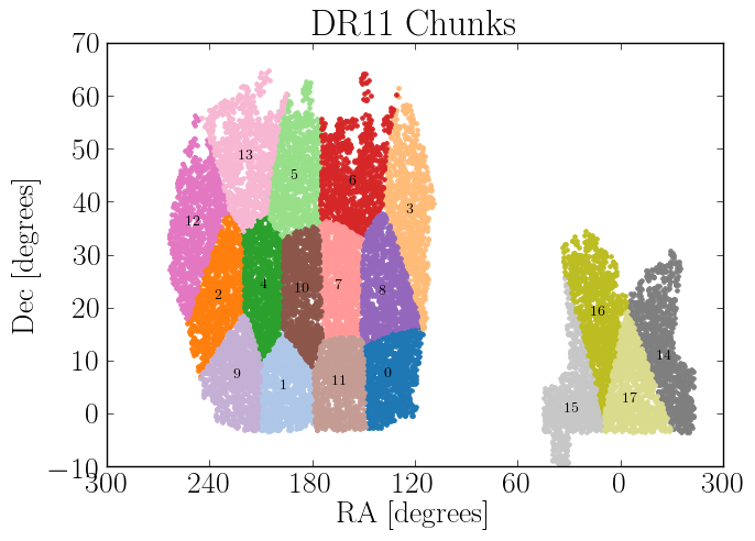
As discussed above, the computational constraints require that the data sample be split into regions with lower numbers of quasars. The DR11 regions were selected by an iterative optimization code designed to make physically compact regions with approximately the same number of QSOs. These regions are shown in the left panel of figure 1.
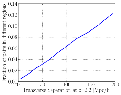
Because the regions are treated independently, the procedure generates no correlations between neighboring quasars that happen to fall in different regions. The right panel of Fig. 1 shows the fraction of QSO pairs which come from different regions as a function of the transverse separation of Ly forest pixels at redshift . For the 3D correlation function, this corresponds to an effective number of pixel pairs in the mocks that is lower than in the data, and this fact needs to be taken into account when comparing mock with data measurements.
3 Generation of expanded mock spectra
In the previous section we described the process of generating the “raw” mock spectra consisting of the correlated transmitted flux fraction along quasar lines-of-sight as defined by eqn. 1.1. In this section we describe the production of so-called “expanded mock spectra” which superimpose the raw spectra on quasar continua and then add astrophysical features such aa high column density absorbers and metal absorption lines, as well as instrumental features such as noise, spectro-photometric calibration errors and sky subtraction residuals.
The mock data are intended to mimic BOSS coadded spectra, which result from the addition of several successive 20-minute individual exposures of the same object, in a given plate and a single night444Under normal observing conditions, the number of exposures for a field is increased until the signal-to-noise of the coadded image reaches a target value.. Most of our discussion below refers to coadded spectra except for the section on noise properties where a distinction between the noise in each exposure and the noise in the coadds is necessary.
For a given quasar, the generated flux is (dropping the quasar index for clarity)
| (3.1) |
The parameters on the right-hand side are as follows: is the transmission fraction as defined by eqn. 1.1 except that it is set to 1 outside the Ly forest; is the PCA-generated quasar continuum; is the Fourier transform of the BOSS resolution and pixelization kernel (eq. 3.2) which is convolved with the product ; is the noise computed from our model (eq. 3.4); is a linear function of (eq. 3.3) used to ensure that each mock spectrum has the same mean flux and spectral index as the corresponding real spectrum; and is the added sky subtraction residuals (fig. 4).
The procedure for generating the correlated Ly transmission field yields a mean absorption and variance given by equations 2.3 and 2.4. That transmission field models regions of optically thin neutral hydrogen absorption, ignoring high-density systems and non-Ly absorbers. In the following two subsections, we describe how we add to these additional absorbers. In the subsequant subsections we describe how we generate the other factors in (3.1) necessary to produce the expanded mock spectra.
3.1 High column density (HCD) systems
Dense systems with high neutral hydrogen column density produce wavelength intervals of complete absorption surrounded by damped wings. These structures affect the measured Ly transmission correlations in two ways. First, they affect the size of the Ly forest fluctuations directly impacting the variance in the resulting long-range 3D correlations. Second, since these systems are themselves biased differently than the optically thin regions, they will also affect these correlations themselves.
Damped Ly systems (DLAs) have strong damped wings that allow for their easy identification, but Lyman-limit systems (LLS) of lower column density can also affect the correlations even if their damped wings are weak and individually not detectable.
We insert both LLS and DLAs with neutral hydrogen column densities , which we collectively designate as high column density (HCD) systems, following the procedure that is described in [20]. In brief, HCD systems are distributed only in pixels where the transmission is lower than a certain threshold , defined such that the probability to have an optical depth larger than is 1%. The column density of the HCD systems are randomly drawn from an analytical model [21] calibrated to match observations [22] from SDSSII-DR7. Voigt profiles [23] are included in these regions assuming a constant Doppler parameter .
3.2 Metals
In addition to absorption from hydrogen, metals in the intergalactic medium can also absorb quasar light at discrete wavelengths inside the Ly forest. Metal absorption lines are individually indistinguishable from Ly forest absorption (at BOSS resolution and noise levels). These metals add “unwanted” correlations to our Ly forest data in two ways. First, absorption correlations are imprinted in individual spectra by gas at a given reshift absorbing at more than one wavelength. For example, a gas system with Ly absorption at wavelength will have correlated metal absortption at wavelength , where is the wavelength of any other transition. While this type of correlation is most important within individual spectra, 3D correlations are also generated because neighboring lines of sight sample redshift-correlated gas structures. The second type of correlation results from the fact that all metal species are themselves tracers of large-scale structure [24]. This leads directly to a weak 3D metal autocorrelation superimposed on the dominant Ly autocorrelation. We focus here on the former effect and will explore the latter in a future publication.
We added metal absorption with a procedure that assumes that all significant metal absorption is associated with strong Ly absorption. For each mock spectrum, we considered pixels for which the Ly transmission was below 0.4. For these cases, we decrease the flux by of their corresponding flux bin at wavelength for each metal line.
Application of this method requires a list of significant metal transitions and appropriate values for the absorption flux decrement, . This was done following the procedure of [4] where quasar spectra were stacked after scaling the wavelength of each spectrum so that selected strong absorption is centered at the restframe Ly transition. The stacked spectra then have, necessarily, strong absorption at the , but also absorption lines at wavelengths separated from this feature by , where is the wavelength of absorption by the species responsible for the strong absorption and is the wavelength of absorption of any other absorber. With these stacks, we identified 21 correlated absorption features, 9 of them corresponding to Ly -metal correlations and the others to metal-metal correlations (arising from the strong absorber being due to a metal line rather than to Ly). We designate these metal-metal correlations as “shadows” hereafter [25]. We allowed these flux decrements to vary by performing this procedure for 7 selected bins in simulated Ly forest flux. Measurements of these metal transition flux decrementsare available as part of the MockExpander package (see Appendix A).
Using the line catalog and the deduced flux decrements, we added metal lines (including shadow lines) to the mock spectra. We did this by reducing the flux at 21 separate wavelengths for every strongly absorbed Ly forest pixel. The introduction of shadow lines in this way is unphysical but this method is employed in order to reproduce the full set of 1D absorption correlations in the mock spectra as tested by stacking both mock and observed spectra (see section 4.4). Our algorithm for the addition of metal absorption assumes that all metal absorption can be characterized by its association with Ly forest absorption. The need for these shadow lines indicates that this is not always the case; some strong metal lines occur where little or no Lyman alpha absorption is apparent.
The ascribed metal absorption is fully determined by the mean metal absorption above and so no scatter is added to these flux decrements. This will be refined in a future publication.
3.3 Quasar continua
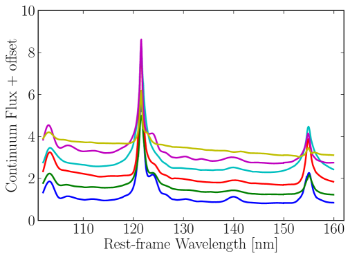
The quasar continuum for each line-of-sight is constructed using eight higher ranked eigenspectra of the Principal Component Analysis (PCA) of low redshift quasar spectra555Low redshift quasars have less absorption in the forest, simplifying the continuum estimation. [26]. The final continuum is a sum of a mean shape and a linear combination of these eigenspectra for which amplitudes were randomly sampled following a centered Gaussian distribution with the corresponding standard deviation. These eigenspectra cover restframe wavelengths 102–160 nm spanning from the Lyman- peak through C IV . Wavelengths above and below this range are discarded in the mock spectra. Figure 2 shows 5 examples of mock continua with variations in line shapes and the shape of the continuum within the Ly forest. The random sampling of the PCA eigenvalue amplitudes occasionally leads to negative continua at some wavelength bins (this happens on 0.5% of the continua), and in this case the continuum is discarded and a new set of random amplitudes is drawn.
3.4 The BOSS kernel
BOSS spectrographs cover the wavelength range 361 nm - 1014 nm with a resolving power varying from in the blue end to in the red end. Each data spectrum has its own estimate of the wavelength dispersion per pixel. In BOSS coadded data, the pixels are logarithmic in wavelength with steps of corresponding to .
As described in section 2, the raw absorption fields were produced over the lines-of-sight using a grid in comoving space with bins of 0.5. To match BOSS spectra binning and resolution, we first compute the mean wavelength dispersion (PSF) and mean pixel width over the Ly forest region of the corresponding data spectrum. Each raw field was then convolved using the following kernel (in Fourier space):
| (3.2) |
We then match the binning by taking, for each data pixel, the absorption value of the closest pixel of the smoothed raw field.
3.5 Flux normalization
We wish to ensure that each mock quasar has a mean forest flux and spectral index equal to those of the corresponding real quasar. Specifically, we normalize the noise-free mock quasar flux to the data flux by fitting for and in
| (3.3) |
over the rest-frame wavelength ranges nm (inside the Ly forest) and nm (between the Ly and CIV emission peaks). Then, is multiplied by the factor . These fits are done using the inverse variance given by the pipeline as fit weights and ignoring all masked pixels. For DR9 mock data-sets, the fit was performed without weighting leading a slightly larger number of bad fits, about 1% of the full sample.
The parameter effectively corrects for quasar spectral distortions introduced by the SDSS optics that are currently not corrected by the pipeline. The Sloan 2.5-m telescope has a chromatic focal plane and lacks an atmospheric dispersion corrector. As a result, the optimal position for a spectrograph fiber is a wavelength and airmass dependent quantity. Galaxy targets and calibration stars are optimized for 540 nm, while quasar targets are offset both along and across the focal plane to optimize the signal-to-noise at 400 nm for Ly forest studies. This offset means that the flux calibration vectors derived from the standard stars are not correct for the quasars and result in a flux mis-calibration which depends upon wavelength, airmass, seeing, guiding, and the location on the focal plane [1].
3.6 The noise,
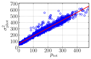
The noise, , added to the fluxes of a given mock quasar is a random number taken from a Gaussian distribution of mean zero and with a variance determined by the noise model for the corresponding real quasar. The noise models are most naturally expressed using the total number of photo-electrons in a given pixel (object plus sky), since in an ideal system the variance would be equal to (pure Poisson noise). In practice, our model gives the variance as a linear function of :
| (3.4) |
The coefficient reflects the CCD readout noise and other systematic effects that are independent of the photon flux. The coefficient would be unity for pure Poisson photon noise in the absence of systematics, but in practice owing to sky subtraction and flux calibration errors.
For each mock quasar, the parameters and are found by fitting as a function of for the corresponding real quasar. This requires the use of a effective calibration vector to transform observed fluxes into photo-electrons:
| (3.5) | |||||
| (3.6) |
where is the estimated flux variance of the data. We fit the linear noise model (Eq. 3.4) for each spectrum, using pixels from the blue side of the spectrograph. Fig. 3 shows an example of a fit for and for one quasar spectrum in DR11.
In addition to , we also need the effective calibration vector in Eqs. 3.5 and 3.6. The BOSS data individual exposures include the calibration vector that converts between observed photo-electrons and calibrated flux . The coadd is performed as a weighted simultaneous spline fit to the individual exposures and the resulting effective calibration vector is not calculated. We re-derive the effective calibration vector using the approximation that the coadded photo-electrons are the unweighted sum of the individual exposure photo-electrons: , where corrects for the wavelength dependent difference in bin-size between individual exposures and the coadded spectra.
Since the coadded flux is normalized to the same units as the individual exposures (ergs/s/cm2/Å), we may factor out such that . Thus the effective calibration vector to convert between coadded photo-electrons and coadded flux is:
| (3.7) |
For this calculation we use only the blue exposures, therefore limiting the wavelength range of mock spectra from to nm.
With the parameters and for each quasar, it is simple to add realistic noise to the mock spectra. We compute the mock quasar flux from the product of the transmission and the generated PCA quasar continuum , and add the same sky flux that is used in the data. We then compute the mock photons and noise at each pixel,
| (3.8) | |||||
| (3.9) |
We add noise using a Gaussian distribution with mean 0 and sigma :
| (3.10) |
We convert back into quasar flux :
| (3.11) |
| (3.12) |
The next step consists in mis-reporting the value of the true variances , as we observe in real data. Biased estimates of pixel variances on real data were reported by different studies [27, 28]. They find that for individual exposures, the pipeline noise estimates are accurate at the 1–2% level. Coadded spectra have a larger and wavelength dependent error in the estimated noise. For nm (blue spectrographs), the biases are approximately proportional to the square root of the ratio of the coadd to individual spectrum spectral bin sizes. Below (above) 475.0 nm, where the coadded bins are smaller (larger) than the original exposures, the pipeline underestimates (overestimates) the noise by 0–10% (0–15%). A flux-dependent bias of the pixel variances was also reported in [28]. We use the observed wavelength dependent errors in the pixel variances to purposefully mis-report the noise in mock spectra.
We also add Gaussian random fluctuations to this noise estimates with standard deviation proportional to the photon variance itself. The final mock photon noise estimate is given by .
The model presented here assumes that the noise in different pixels of the same spectrum is uncorrelated. This is likely not realistic because covariance among neighboring pixels is introduced by rebinning. However, other sources of small scale correlations in these mock catalogs are not correctly modeled by the input power spectrum, since the log-normal model was built to fit large-scale correlations. Therefore we ignore any noise correlation between neighboring bins.
An alternative noise model [29] uses four per-object parameters (instead of two in our model). This method solves simultaneously for both the noise parameters and the optimal co-added flux. However, this modeling is inappropriate for our current purposes since our goal is to add noise to the mock co-added flux, which follows the pipeline and is not optimal.
3.7 Sky mis-subtraction
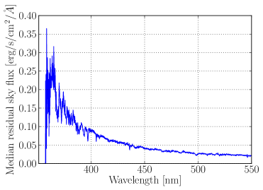
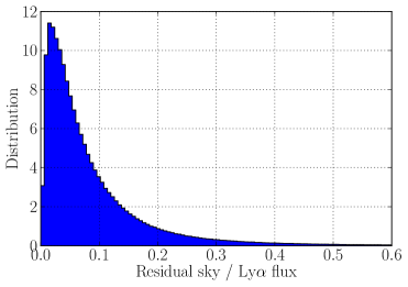
Figure 4 (left) shows the median residual of BOSS sky spectra after the sky model has been subtracted. While this is only a 1–2% bias in the sky subtraction, it can be large compared to the Ly forest flux, which is typically faint compared to the sky. Fig. 4 (right) shows the relative flux between noise-free simulated Ly forest flux and the residual sky. The median is , the mean is , and there is a tail reaching up to 1.0. Note that this is an additive component to mock spectra, unlike other mis-calibrations that are multiplicative.
Mock spectra add this median sky subtraction residual times a random constant scatter with mean 1.0 and RMS 0.1 so that each spectrum receives a slightly different sky subtraction residual bias.
4 Comparisons of mock and real spectra
In this section we compare several properties of the mock spectra to those of real spectra: continuum characteristics, noise levels, flux transmission correlations within individual spectra, and absorption by metals. Unless otherwise stated, the standard set of mocks used for the comparisons in this section does not contain metals or high column density systems (HCDs), but includes all instrumental systematics. The effect of metals and HCDs is studied in the end of section 5.1.
4.1 Mean continuum, variance and diversity
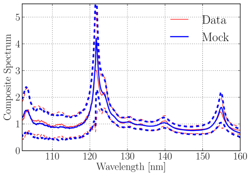
As a first test, we compare the mean spectra of the data and mocks. This simple test verifies that the product of mean continuum and forest transmission is reasonable. The mean spectra were calculated by first shifting each spectrum to its rest frame and normalizing it such that the average flux in the wavelength interval from 126 nm to 138 nm is unity. We stacked the set of normalized spectra to obtain the mean product of continuum and transmission and its variance as a function of rest-frame wavelength.
The solid lines in figure 5 shows the resulting mean spectra, red for the data and blue for the mocks. The dashed lines show the flux at one standard deviation higher and lower than the mean. The largest differences are in the height of the Ly emission peak and to a lesser extent in the height of the iron lines in the Ly forest. Whether these differences are an issue or not depends on the application. For instance, the methods in [4, 5, 6, 8] only use the Ly forest for the purposes of measuring the 3D correlation function, and the composite spectrum is computed self-consistently (which would automatically account for the shape differences when analyzing mocks or data).
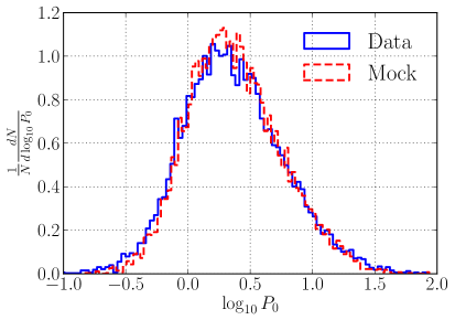
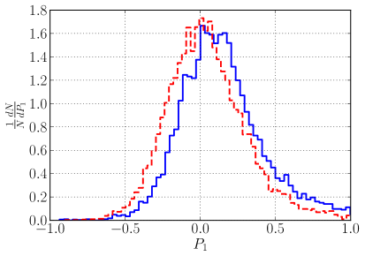
We have also performed a second test of spectral diversity in the region of the forest. For this test, we applied the continuum fitting C2 of [8] and and then fit the observed flux between the upper and lower limits of the forest, and :
| (4.1) |
where is the flux, is the quasar-averaged flux, and are free positive parameters (to ensure a positive continuum). The upper limit is nm and is the larger of 360 nm and nm.
For each forest we define a normalization parameter and a tilt parameter . The distributions of these two parameters are given in figure 6. There is an excellent agreement in the distributions of and in mocks and data. The average value of the tilt is slightly smaller on mocks due to a combination of factors affecting the continuum fitting estimates: differences in the sky residuals, mean transmission and underlying transmission PDF. These factors are hard to estimate accurately from the data and to model in the mocks. The distribution of amplitudes and tilts have similar spreads in mocks and data, demonstrating that our mocks capture the diversity of real data in the region of the Ly forest, at least regarding the spectral index variability.
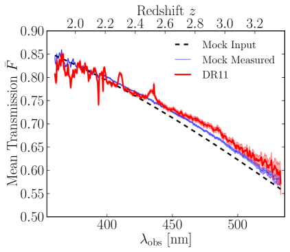
The continuum fitting method C2 of [8] provides an estimate of the unabsorbed continuum, . Stacking spectra in observed wavelength then gives the mean transmission as a function of redshift or, equivalently, of observed wavelength. Figure 7 shows this quantity for the data and mocks. Data reduction features are visible in the data stack (dashed red), such as the galactic calcium absorption (393.4 and 396.8 nm) or the Balmer residuals (near 398 nm, 410 nm and 435 nm). Some of those features are also present in the stack of mocks (solid blue) as a result of the addition of the sky residuals from figure 4 but are not otherwise explicitly included.
4.2 Noise
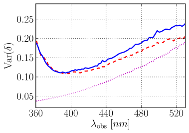
The importance of accurately simulating noise is due to the fact that noise accounts for about one half of the variance of individual measurements of the flux transmission, the other half coming from the intrinsic variations due to large-scale structure. In turn, the variance of individual measurements accounts for about one half of the variance of the measured three-dimensional correlation function with the other half due to correlations between measurements of neighboring pixels on individual spectra.
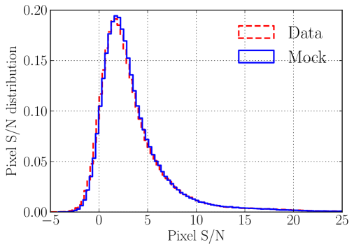
Figure 8 compares the distribution of signal-to-noise ratio for individual pixels in the forest in mocks and data. The signal-to-noise is defined, for each individual pixel, as the ratio between the flux and the square-root of the pipeline estimate of the variance (before applying the corrections discussed in section 3.6). Given that in most studies the spectra are normalized to an unabsorbed continuum estimate, this ratio is the relevant quantity to compare. We find a very good agreement between mocks and data.
Figure 9 shows the variance of the individual measurement of the transmission, , as a function of redshift. It has contributions from noise and large-scale-structure fluctuations. The latter contribution can be computed using noiseless mocks, as is shown by the dotted magenta line. It represents roughly 50% of the total variance. The agreement between mock and data variances is good (few percent level) below nm, which corresponds to a redshift of 2.6, including a considerable fraction of analysis pixels [8]. It is degraded by up to 10-15% up above 480 nm (), beyond which there are very few Ly forest pixels in the BOSS sample.
4.3 Correlations within individual forests
Here we compare the correlations of within individual forests, described by the correlation function:
| (4.2) |
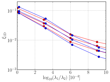
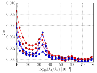
for which we have used the same estimator (Eq. 1.2) and weighting scheme as in [8] but changed the binning to work in wavelength instead of comoving separation. For this comparison, we used mocks including metal absorption. As shown in figure 10, is a rapidly decreasing function of wavelength separation except near where it has a peak due to SiIII absorption correlated with Ly absorption.
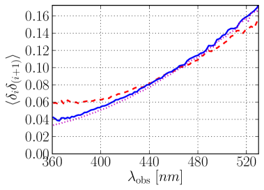
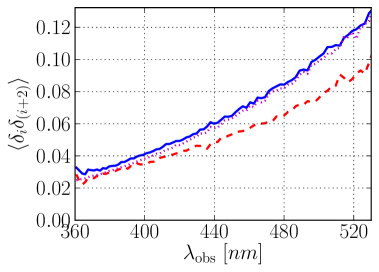
We first discuss for small separations. Figure 11 compares for mocks and data for the first two non-zero separation bins: (left) and (right). In these cases, the blue line (standard mocks) and the magenta line (noiseless mocks) closely follow one another. This is because our model assumes that the noise in different mock pixels is uncorrelated (this is not true for real data). The disagreement between mocks and data is at the 15-20% level and could be due either to an inaccurate input correlation function on small scales, or to inaccurate modeling of the instrument. On the clustering side, the small scales of these mocks are not supposed to be accurately modeled (due to resolution limitations), since the main goal is the large scales and BAO measurement. On the instrumental side, we do not simulate the coaddition process of individual exposures, that introduces correlations among nearest neighboring pixels in real data.
The correlations for larger pixels separations are shown in figure 10 for three redshift bins. Outside the SiIII bump at , the mocks clearly have less correlation than the data. On the bump, the mocks appear to have a much stronger redshift dependence of the absorption.
The disagreement between the data and mock means that the covariance matrices of the two will be slightly different (section 5.2). Given the uncertainties in BAO measurements are dominated by pixel variance and the covariance of neighboring pixels, we will leave these issues to future work.
An alternative way to study correlations within individual spectra is the Fourier transform of , the one-dimensional power spectrum, , a very powerful probe to constraint cosmological models [18, 27]. However, we do not expect that the mocks spectra presented here will give a realistic spectrum for all , especially at small scales where our treatment is rather crude (see section 2). We have also assumed a constant resolution over the whole mock forests.
We computed the 1D power spectrum following the same procedure as in [27] for a sub-sample of 16,000 mock spectra having signal-to-noise ratio greater than 2 and mean resolution below 85 (same cuts as for real data). The flux fluctuations were obtained by dividing out the mean stacked flux over forests. We used a Fast Fourier Transform to convert the fluctuations to -space to estimate the power spectrum. The noise contribution to the power was subtracted, assuming it is constant over . The resolution and pixelization kernel (Eq. 3.2) was also divided out. This measurement was done in four redshift bins equally divided between . We analyzed mock spectra with no noise added (only the continuum multiplied by the absorption field) in order to see effects of binning and resolution on the power.
The analysis on full expanded spectra needs an estimator for the noise mis-estimates. In [27], this estimate was performed using two different procedures, the first uses individual exposures of each spectra, the second uses flat spectral regions redwards of the Ly emission peak. None of these procedures can be applied on mock spectra since individual exposures are not produced, and no quasar with is created meaning that no region of mock spectrum redwards of Ly falls into the blue end of the spectrograph, which would allows us to estimate the true noise. Therefore, the 1D power spectrum measurement on expanded spectra was performed using the true pixel noise, which is constant in -space.
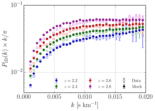
Fig. 12 shows the estimated 1D power spectrum of mock spectra, compared with the measurement performed on DR9 data [27]. The overall shape of power spectra is in good agreement with data. The power spectrum on the lowest redshift bin, , shows the best agreement with data while the higher redshift measurements have up to 20% more power than data on large scales ( s km-1). This increase in power at high redshift is related to the increase in pixel variance observed in Fig. 9. On small scales ( s km-1), data and mocks show an agreement within 1 for most points, but this is due mainly to the large errors on data points. As we saw in the , the clustering on small scales is not correctly modeled in our mocks.
We remind that covariance matrix measurements for BAO in data are not derived from mocks, but from the data itself. Therefore, discrepancies seen here in the small scale clustering does not have an important role in the final measurement.
4.4 Metals
Metal absorption correlated with Ly absorption was included in mock forests following prescription described in section 3.2. In order to test our method of introducing metal absorption, we stacked Ly absorption in our mock forests following a modified method from [30]. In Fig. 13 the resulting stack for Ly transmission values in the range is shown as a function of rest-frame wavelength, in comparison with the stack using real data. Errors were computed by bootstrap. The agreement for most of the lines is at the sub-percent level, in particular for the stronger ones. Similar agreement is also observed in stacks of absorbers with different transmission values ( and ). This validates our implementation, constructed with the purpose of investigating systematic effects of metals on the BAO measurement. The effect of these metals on the correlation function is discussed in section 5.1.

5 Three-dimensional statistical properties of the mock and real spectra
In this section we compare the 3D correlation function of the mock and real spectra and their covariances. We do this first for the mock spectra without high-column-density and metallic absorbers. We then study the effects of of these two absorbers on the measured correlation function.
5.1 Three dimensional correlation function
The correlation function is measured using eqn. 1.2 as a function of the transverse separation () and the parallel separation () between pixels. We organize these data in bins or and (where is the angle between the pixel-separation vector and the line of sight). We finally consider three “wedges” in : , and and compute the average of the correlation function in each wedge as a function of to obtain , and respectively. The three panels in figure 14 show the results. The gray lines correspond to individual mock realizations and illustrate the spread. The blue lines show the mean (solid) and the limits (dashed) for the sample of mocks. The red points with error bars are the results from the data [8].
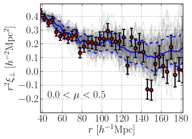
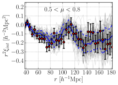
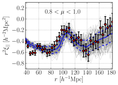
The agreement between the mocks and data is good. The most noticeable difference is a mismatch in the position of the BAO peak in . This difference is characterized in [8] as a discrepancy between the predicted position of the BAO peak by the fiducial cosmology of the mocks and that measured from data.
5.2 Covariance.
The covariance matrix of the 3D correlation function bins can be estimated directly from the data using the subsampling technique developed in [8]. This internally estimated covariance for a given mock can be compared with the variability among the 100 mock realizations characterized by its variance:
| (5.1) |
where is the number of mocks (100) is the 3D correlation function measured at a separation bin and is the average correlation function in the mocks sample. Since non-diagonal correlations are too small to estimate with only 100 mocks, we only compare the variances.
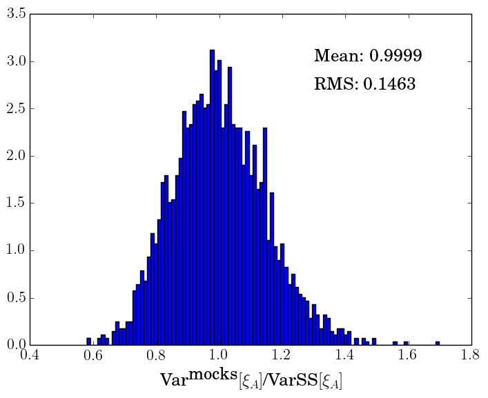
Figure 15 shows a histogram of the ratio of variances estimated using equation 5.1 and that obtained using the subsampling method from [8]. The agreement between both calculations of the variance is excellent. This validates our methods to compute the covariance matrix, showing the importance of this set of mock catalogs for the measurement on real data.
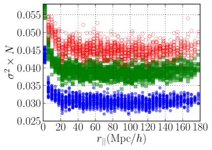
Next we compare the variances in mocks and data. Since the number of quasars in the mocks is not exactly the same as in real data, we compare the product of the variance and the number of pairs for each bin in separation. Figure 16 shows the product of the variance and the number of pairs as a function of transverse separation for data (in red) and mocks (in blue). This figure shows that the mocks have 30% less variance than the data. This difference may come from the differences in the one-dimensional correlation function (see figure 9).
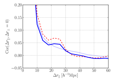
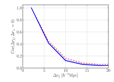
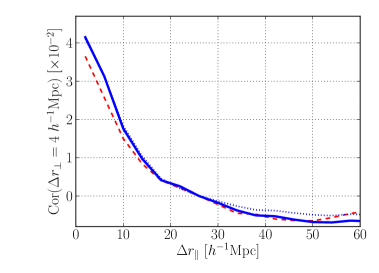
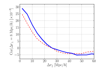
We also compared non-diagonal terms of the covariance matrix. Following [8], we assume that this matrix is a function of and , and thus compute of the average of all correlation coefficients (covariance normalized by the geometric mean of variances) with same and . In figure 17, we plot these averaged correlations as a function of for the three first transverse bins, and 8 . In the first transverse bin, where the covariance matrix is determined by the line-of-sight correlation function, we clearly see a peak at corresponding to Ly-SiIII correlations. This peak is, as expected, absent from the covariance matrix of metal-less mocks. As before, data shows slightly more correlation on small scales. The covariance falls quickly to zero as increases. For these bins, data and mock non-diagonal terms of the covariance matrix generally agree in shape but data shows smaller correlation coefficients likely due to the differences in the one-dimensional correlation function.
5.2.1 Effect of Lyman-limit systems.
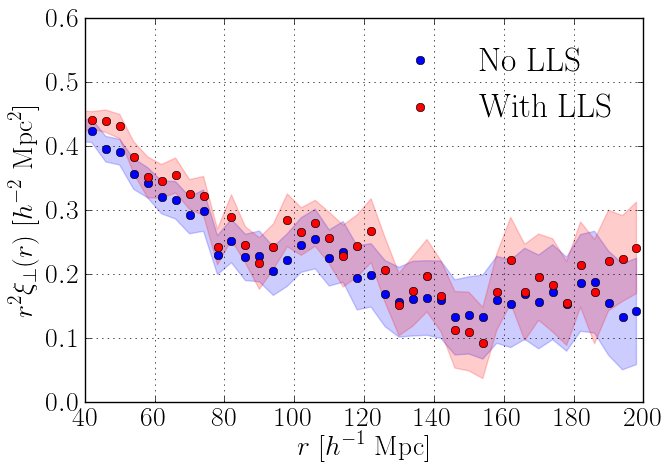
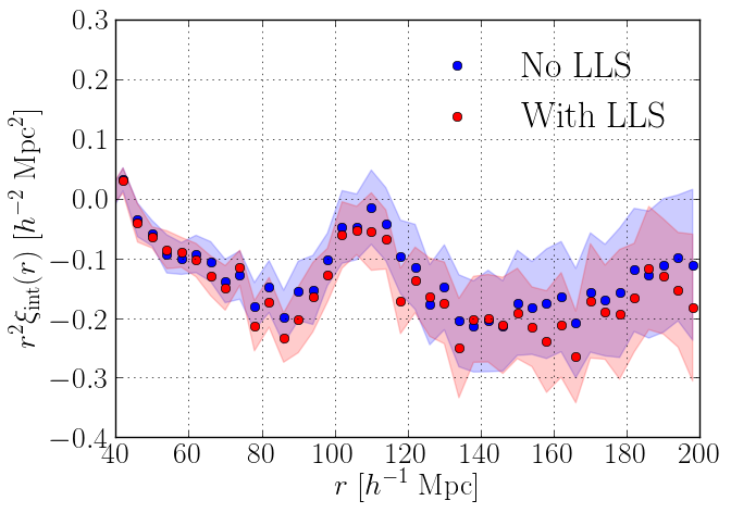
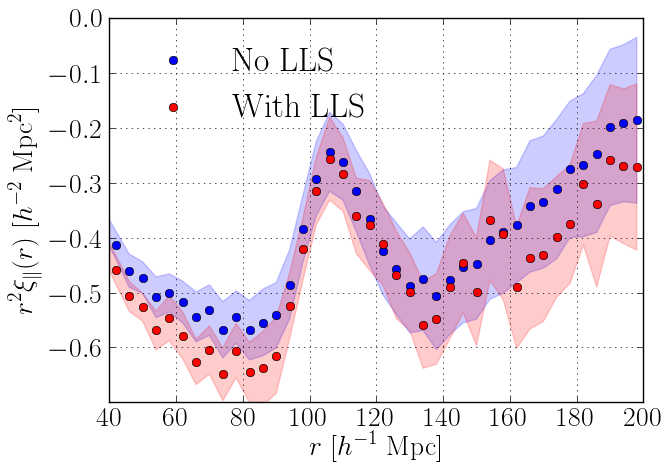
Thus far, the comparison has been performed using mock catalogs with no high-column density absorbers even though they are present in data. In this section we see the effect of adding Lyman-limit systems (LLS) to the spectra. Since DLAs can be identified in the data and treated separately, we excluded from our analyses all forests containing DLAs (), while conserving forests with LLS (). In Fig. 18 the stacked 3D correlation function of mocks containing LLS is compared with the stack of realizations without them. As already observed by [20], the inclusion of high column density systems increases the bias of the correlation function. This is now shown also taking into account the BOSS spectrograph properties and using the standard BAO Ly analysis. This effect comes from the increased absorption from LLS that reduces the mean transmission and also increases the intrinsic variance of the absorption field. The increase in bias of the correlation function depends on two factors. First it depends on the number density of these systems and the dependence of this number with redshift. Second, it depends on how these systems are related to the underlying density field. On real data, the distribution of Lyman limit systems is not known to high precision [31], therefore the used input mock LLS distribution might not be accurate. Furthermore, due to our method of including LLS on forests (see section 3.1), the redshift distortion parameter for LLS, , is the same as for the Ly forest, , which is also an approximation (we expect that ). Therefore quantitative results of their effects on the correlation function are not reliable, even though their qualitative effect is correct. It is important to remark in Fig. 18 that these systems do not change the position of the BAO peak or its width. However, measuring bias or redshift space distortions need to carefully take into account the additional clustering coming from Lyman limit systems.
5.2.2 Effect of metals.
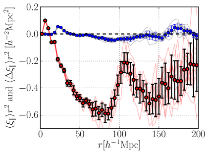
In addition to Lyman limit systems, real forests also contain metal absorption that cannot be identified due to the low signal-to-noise of spectra or confusion between source transitions. We included metal absorption in mock spectra (see section 3.2) and we found that their effect on the correlation function and its errors is smaller than the effect of LLS. The main effect of metal absorption is seen on correlations of pixels with separations nearly aligned to the line-of-sight (), on bins with small transverse separation (). Figure 19 shows the difference between correlations of metal and metal-less mocks (blue points) compared with mean correlation function (red points), computed using 10 mock realizations. In addition to the Ly-SiIII line (see Fig. 13), the effect of the SiII-SiIII shadow line is also visible on the 3D correlation for and . Since bins for which contain small number of pairs compared to bins at larger transverse separations, the presence of metal correlations on large scales do not bias BAO fitting procedures (Fig. 12 of [8]).
6 Discussion & Conclusions
In this paper, we have presented the mock Ly forest catalogs for the Data-Release 11 of the SDSS-III. These mock spectra have been a fundamental tool for validating methods of the main BOSS Ly BAO measurements [5, 6, 7, 8].
The analysis of the mocks presented in Section 5 shows that they reproduce well the observed correlation function of the transmission fluctuations as measured in [8]. The measured covariance matrix of the mock correlation function is comparable to that of the real data but does show systematic deviations for both the variance and the off-diagonal elements. As long as the errors are used in a consistent manner, these differences do not prevent the mock spectra from being useful to verify that the analysis returns reasonable values for the statistical errors and to show that there are no obvious biases in the measured position of the BAO peak.
The deviations between mock and data covariances matrices reflect the statistical properties of individual mock spectra which, as shown in Section 4, differ from the real spectra. The differences are due to the necessarily approximate treatment of the input power spectrum at small scales. We have not simulated all the imperfections in the BOSS pipeline, in particular the presence of Balmer artifacts. We can anticipate, however, that these artifacts will be removed with future improvements in the pipeline.
Of more fundamental concern is the uncertain nature of the correct way of introducing high column density systems and metallic absorbers. Improvements in these aspects of the simulations will require further study.
Acknowledgments
This research used resources of the National Energy Research Scientific Computing Center (NERSC), which is supported by the Office of Science of the U.S. Department of Energy under Contract No. DE-AC02-05CH11231.
The authors acknowledge the support of France Grilles for providing computing resources on the French National Grid Infrastructure.
This project was supported by the Agence Nationale de la Recherche under contract ANR-08-BLAN-0222. The research leading to these results has received funding from the European Union Seventh Framework Programme (FP7/2007-2013) under grant agreement n [PIIF-GA-2011-301665].
This work has been carried out thanks to the support of the A*MIDEX project (ANR-11-IDEX-0001-02) funded by the “Investissements d’Avenir” French Government program, managed by the French National Research Agency (ANR).
Funding for SDSS-III has been provided by the Alfred P. Sloan Foundation, the Participating Institutions, the National Science Foundation, and the U.S. Department of Energy Office of Science. The SDSS-III web site is http://www.sdss3.org/.
SDSS-III is managed by the Astrophysical Research Consortium for the Participating Institutions of the SDSS-III Collaboration including the University of Arizona, the Brazilian Participation Group, Brookhaven National Laboratory, University of Cambridge, Carnegie Mellon University, University of Florida, the French Participation Group, the German Participation Group, Harvard University, the Instituto de Astrofisica de Canarias, the Michigan State/Notre Dame/JINA Participation Group, Johns Hopkins University, Lawrence Berkeley National Laboratory, Max Planck Institute for Astrophysics, Max Planck Institute for Extraterrestrial Physics, New Mexico State University, New York University, Ohio State University, Pennsylvania State University, University of Portsmouth, Princeton University, the Spanish Participation Group, University of Tokyo, University of Utah, Vanderbilt University, University of Virginia, University of Washington, and Yale University.
References
- [1] K. S. Dawson, D. J. Schlegel, C. P. Ahn, et al., The Baryon Oscillation Spectroscopic Survey of SDSS-III, AJ 145 (Jan., 2013) 10, [arXiv:1208.0022].
- [2] D. J. Eisenstein, D. H. Weinberg, E. Agol, et al., SDSS-III: Massive Spectroscopic Surveys of the Distant Universe, the Milky Way, and Extra-Solar Planetary Systems, AJ 142 (Sept., 2011) 72–+, [arXiv:1101.1529].
- [3] É. Aubourg, S. Bailey, J. E. Bautista, et al., Cosmological implications of baryon acoustic oscillation (BAO) measurements, ArXiv e-prints (Nov., 2014) [arXiv:1411.1074].
- [4] A. Slosar, A. Font-Ribera, M. M. Pieri, et al., The Lyman- forest in three dimensions: measurements of large scale flux correlations from BOSS 1st-year data, JCAP 9 (Sept., 2011) 1–+, [arXiv:1104.5244].
- [5] N. G. Busca, T. Delubac, J. Rich, et al., Baryon acoustic oscillations in the Ly forest of BOSS quasars, Astron. Astrophys. 552 (Apr., 2013) A96, [arXiv:1211.2616].
- [6] A. Slosar, V. Iršič, D. Kirkby, et al., Measurement of baryon acoustic oscillations in the Lyman- forest fluctuations in BOSS data release 9, JCAP 4 (Apr., 2013) 26, [arXiv:1301.3459].
- [7] D. Kirkby, D. Margala, A. Slosar, et al., Fitting methods for baryon acoustic oscillations in the Lyman- forest fluctuations in BOSS data release 9, JCAP 3 (Mar., 2013) 24, [arXiv:1301.3456].
- [8] T. Delubac, J. E. Bautista, N. G. Busca, et al., Baryon acoustic oscillations in the Lyα forest of BOSS DR11 quasars, Astronomy and Astrophysics 574 (Feb., 2015) A59.
- [9] Planck Collaboration, P. A. R. Ade, N. Aghanim, et al., Planck 2013 results. XVI. Cosmological parameters, ArXiv e-prints (Mar., 2013) [arXiv:1303.5076].
- [10] R. Cen, J. Miralda-Escudé, J. P. Ostriker, and M. Rauch, Gravitational collapse of small-scale structure as the origin of the Lyman-alpha forest, Astrophys. J. Let. 437 (Dec., 1994) L9–L12.
- [11] P. Petitjean, J. P. Mueket, and R. E. Kates, The LY alpha forest at low redshift: Tracing the dark matter filaments, Astron. Astrophys. 295 (Mar., 1995) L9–L12, [astro-ph/9502100].
- [12] J. Miralda-Escudé, R. Cen, J. P. Ostriker, and M. Rauch, The LY alpha Forest from Gravitational Collapse in the Cold Dark Matter + Lambda Model, Astrophys. J. 471 (Nov., 1996) 582–+.
- [13] P. McDonald, Toward a Measurement of the Cosmological Geometry at z ~ 2: Predicting Ly Forest Correlation in Three Dimensions and the Potential of Future Data Sets, Astrophys. J. 585 (Mar., 2003) 34–51, [astro-ph/0].
- [14] G. Rossi, N. Palanque-Delabrouille, A. Borde, et al., A Suite of Hydrodynamical Simulations for the Lyman-Alpha Forest with Massive Neutrinos, ArXiv e-prints (Jan., 2014) [arXiv:1401.6464].
- [15] A. Font-Ribera, P. McDonald, and J. Miralda-Escudé, Generating mock data sets for large-scale Lyman- forest correlation measurements, JCAP 1 (Jan., 2012) 1, [arXiv:1108.5606].
- [16] A. Font-Ribera, D. Kirkby, N. Busca, et al., Quasar-Lyman $alpha$ Forest Cross-Correlation from BOSS DR11 : Baryon Acoustic Oscillations, ArXiv e-prints (Nov., 2013) [arXiv:1311.1767].
- [17] A. Lewis, A. Challinor, and A. Lasenby, Efficient Computation of Cosmic Microwave Background Anisotropies in Closed Friedmann-Robertson-Walker Models, Astrophys. J. 538 (Aug., 2000) 473–476.
- [18] P. McDonald, U. Seljak, S. Burles, et al., The Ly Forest Power Spectrum from the Sloan Digital Sky Survey, ApJS 163 (Mar., 2006) 80–109, [astro-ph/0].
- [19] A. S. Bolton, D. J. Schlegel, É. Aubourg, et al., Spectral Classification and Redshift Measurement for the SDSS-III Baryon Oscillation Spectroscopic Survey, AJ 144 (Nov., 2012) 144, [arXiv:1207.7326].
- [20] A. Font-Ribera and J. Miralda-Escudé, The effect of high column density systems on the measurement of the Lyman- forest correlation function, JCAP 7 (July, 2012) 28, [arXiv:1205.2018].
- [21] Z. Zheng and J. Miralda-Escudé, Self-shielding Effects on the Column Density Distribution of Damped Ly Systems, Astrophys. J. Let. 568 (Apr., 2002) L71–L74.
- [22] P. Noterdaeme, P. Petitjean, C. Ledoux, and R. Srianand, Evolution of the cosmological mass density of neutral gas from Sloan Digital Sky Survey II - Data Release 7, Astron. Astrophys. 505 (Oct., 2009) 1087–1098, [arXiv:0908.1574].
- [23] J. J. Olivero and R. L. Longbothum, Empirical fits to the Voigt line width: A brief review, Journal of Quantitative Spectroscopy and Radiative Transfer 17 (Feb., 1977) 233–236.
- [24] M. M. Pieri, The C IV forest as a probe of baryon acoustic oscillations, Mon. Not. Roy. Astron. Soc. 445 (Nov., 2014) L104–L108, [arXiv:1404.4569].
- [25] M. M. Pieri, S. Frank, D. H. Weinberg, S. Mathur, and D. G. York, The Composite Spectrum of Strong Ly Forest Absorbers, Astrophys. J. Let. 724 (Nov., 2010) L69–L73, [arXiv:1001.5282].
- [26] N. Suzuki, D. Tytler, D. Kirkman, J. M. O’Meara, and D. Lubin, Predicting QSO Continua in the Ly Forest, Astrophys. J. 618 (Jan., 2005) 592–600.
- [27] N. Palanque-Delabrouille, C. Yèche, A. Borde, et al., The one-dimensional Ly forest power spectrum from BOSS, Astron. Astrophys. 559 (Nov., 2013) A85, [arXiv:1306.5896].
- [28] K.-G. Lee, S. Bailey, L. E. Bartsch, et al., The BOSS Ly Forest Sample from SDSS Data Release 9, AJ 145 (Mar., 2013) 69, [arXiv:1211.5146].
- [29] K.-G. Lee, J. P. Hennawi, D. N. Spergel, et al., IGM Constraints from the SDSS-III/BOSS DR9 Ly-alpha Forest Flux Probability Distribution Function, ArXiv e-prints (May, 2014) [arXiv:1405.1072].
- [30] M. M. Pieri, M. J. Mortonson, S. Frank, et al., Probing the circumgalactic medium at high-redshift using composite BOSS spectra of strong Lyman forest absorbers, Mon. Not. Roy. Astron. Soc. 441 (June, 2014) 1718–1740, [arXiv:1309.6768].
- [31] M. McQuinn, S. P. Oh, and C.-A. Faucher-Giguère, On Lyman-limit Systems and the Evolution of the Intergalactic Ionizing Background, Astrophys. J. 743 (Dec., 2011) 82, [arXiv:1101.1964].
Appendix A Access and usage of mocks
The DR11 Ly forest mock catalogs are available at the SDSS public website http://www.sdss.org/dr12/algorithms/lyman-alpha-mocks/. We describe in this section the mock data-sets format and their usage. Instead of providing the full set of realizations containing spectra ready to use, i.e., realizations with continua, noise and instrumental effects, only the raw absorption fields are provided. The “expansion” process is performed locally by the LyAMockExpander package, available in http://www.sdss3.org/svn/repo/boss/LyAMockExpander/. This procedure reduces the amount of data that needs to be transferred, and gives the user the possibility of including or not some systematic effects.
A.1 Raw mock data format
The first step consists in downloading raw mock fiels, containing absorption fields and high column density system information. A given raw file for a given spectrum is named: mockrawShort-PLATE-MJD-FIBER.fits. It contains a certain number of realizations of the same line of sight.
This file is organized as follows:
-
•
HDU 0: header propagated form the real spectrum file, with additional information concerning the mock production (cosmological model and Ly forest clustering parameters). Mock related keywords are:
M_Z Mock redshift M_RA Mock RA [degrees] M_DEC Mock dec [degrees] M_OMEGAM Mock Matter fraction M_OMEGAK Mock Curvature parameter M_W Mock Dark-energy equation of state M_H Mock Hubble constant M_NS Mock Primordial scalar spectral index M_BIAS Mock Ly forest bias w.r.t. linear dark-matter power-spectrum M_BETA Mock Ly forest redshift distortion parameter M_ALPHA Mock Ly forest redshift evolution parameter M_NEVOL Mock number of redshift evolution steps M_DV Mock grid spacing in km/s at NMOCKS Number of mock realizations in this file -
•
HDU 1 to NMOCKS: binary tables containing the absorption field for each realization.
f the transmittance of the Ly forest fdla the same as above but containing HCD profiles -
•
HDU NMOCKS+1 to 2*NMOCKS: binary tables containing information about HCDs of the realizations.
x_dla the comoving position of the system z_dla the corresponding redshift of the system col_dla the column density of the absorber, in cm-2.
For DR11, the 100 realizations of a given forest are divided in 10 different files, containing 10 realizations each.
A.2 MockExpander
This package transforms raw absorption fields into quasar spectra including astrophysical and instrumental effects characterized in BOSS data.
The MockExpander was developed and compiled in JAVA language, and it is a stand alone, open-source version. The user chooses expansion options in the Run.sh script. We summarize these options here:
-
•
Raw_Mock_Directory: the folder containing the raw format files
-
•
Data_Directory: the folder containing the data spectra, containing individual exposures, in spec666http://data.sdss3.org/datamodel/files/BOSS_SPECTRO_REDUX/RUN2D/spectra/PLATE4/spec.html format.
-
•
Output_Directory: the folder were the MockExpander will write the output mock files.
-
•
Package_Seed: sets the random number generator seed based on which set of realizations.
-
•
Initial(Final)_Realization : the user might want to expand a sub-set of the available realizations, these keywords allow the user to choose them, using their position in the file (1 to NMOCKS).
-
•
ACTION: This option allows the user to choose between start the expansion again (“Rewrite”) overwriting previous files, or continue (“Continue”) from the last mock produced.
-
•
COOKING: Set if the expansion will include high column density systems and/or metal absorption.
-
•
COLS: the user can choose the output columns of the expanded mock data-sets. They are fully described in Table 1.
Once options are chosen, the user executes the Run.sh script to start the expansion.
A.3 Expanded mocks data format
The final output is a per-object FITS file in the same format as real BOSS data. The guiding principle is that if an analysis code can use the real data, it should also be able to use the mock data without requiring any changes other than the input file names.
Mock files also contain additional information used in their construction. Table 1 describes the content of HDU1. HDUs 0 (observing headers) and 2 (metadata) are simply copies of the corresponding HDUs from the real data files. Mock files do not receive HDU 3 from real data (emission line fits and individual exposures). Instead, HDU 3 contains the location of the high column density systems (it is a copy of corresponding raw format HDU).
| Column | Comment | Symbol |
| In both mocks and real data: | ||
| flux | coadded calibrated flux [10-17 ergs/s/cm2/Å] | |
| loglam | (wavelength [Å]) | |
| ivar | inverse variance of flux | |
| and_mask | mask | - |
| or_mask | mask | - |
| wdisp | wavelength dispersion in dloglam units | |
| sky | subtracted sky flux [10-17 ergs/s/cm2/Å] | |
| model | pipeline best model fit used for classification | - |
| and redshift | ||
| Only in the mocks: | ||
| mock_F | transmitted flux fraction [0–1] | |
| mock_Fdla | transmitted flux fraction with Damped Ly systems | |
| mock_Fmet | transmitted flux fraction with metal absorption | |
| mock_Fdlamet | transmitted flux fraction with Damped Ly systems | |
| and metal absorption | ||
| mock_meanF | Mean transmitted flux fraction | |
| mock_ivar | True inverse variance used to add noise | |
| mock_contpca | the PCA-based continuum model | |
| noise_miscalib | amount by which reported noise is wrong. | |
| means noise is underestimated. | ||
| mock_miscalib | amount by which the flux is purposefully miscalibrated | |
| mock_missky | amount of extra sky added to simulated sky mis-subtraction | |
The MockExpander will automatically organize output files in a per-realization and a per-plate folder scheme as for real data.