Equation-of-State Parameter for Reheating

Abstract

Constraints to the parameters of inflation models are often derived assuming some plausible range for the number—e.g., $N_{k}=46$ to $N_{k}=60$—of $e$-folds of inflation that occurred between the time that our current observable Universe exited the horizon and the end of inflation. However, that number is, for any specific inflaton potential, related to an effective equation-of-state parameter $w_{\mathrm{re}}$ and temperature $T_{\mathrm{re}}$, for reheating. Although the physics of reheating is highly uncertain, there is a finite range of reasonable values for $w_{\mathrm{re}}$. Here we show that by restricting $w_{\mathrm{re}}$ to this range, more stringent constraints to inflation-model parameters can be derived than those obtained from the usual procedure. To do so, we focus in this work in particular on natural inflation and inflation with a Higgs-like potential, and on power law models as limiting cases of those. As one example, we show that the lower limit to the tensor-to-scalar ratio $r$, derived from current measurements of the scalar spectral index, is about 20%-25% higher (depending on the model) with this procedure than with the usual approach.

I Introduction

Models of inflation that rely on the slow rolling of a single scalar field have become the canonical family of models for inflation Linde:1983gd ; 0811.1989 ; 1404.1065 . These models are specified by a potential-energy density $V(\phi)$ given as a function of the inflaton field $\phi$. As long as the slow-roll conditions, which require that the slope and curvature of $V(\phi)$ are sufficiently small, are satisfied, the Universe inflates. Inflation then ends and is followed by a period of reheating (see Ref. Allahverdi:2010xz for a review) that converts the energy density in the inflaton to the thermal bath, at a reheating temperature $T_{\mathrm{re}}$, that fills the Universe at the beginning of the standard radiation-dominated epoch.

In the canonical reheating scenario elementary-theory , oscillations of the inflaton around the minimum of its potential correspond to massive inflaton particles, and these particles then decay to the plasma of Standard Model particles that compose the radiation-dominated Universe. However, the physics of reheating may be far more complicated. For example, different rates for different types of decays into different Standard Model particles may yield different clocks for starting the usual radiation-dominated epoch. There may be a preheating stage 1410.3808 , where there is a resonant production of particles Kofman:1994rk , which can enhance the inflaton decay via scattering hep-ph/9704452 , or where inhomogeneous modes may be excited hep-ph/9705357 . Turbulence may also play a role turbulent-thermalization . It is generally assumed that the reheat temperature is above the electroweak transition (presumably so that weak-scale dark matter can be produced). More conservatively, though, the reheat temperature must be above an MeV, the temperature of big-bang nucleosynthesis, the earliest time for which we have clear empirical relics. The theoretical uncertainty in reheating is often taken into account, in the consideration of experimental constraints to inflation models, by surmising some reasonable range—e.g., $N_{k}=46$ to $N_{k}=60$—for the number $N_{k}$ of $e$-folds of inflation between the time that our observable horizon exited the horizon during inflation and the end of inflation. The upper limit to this range arises if inflaton oscillations reheat the Universe instantaneously to a grand unified theory-scale temperature, and the lower limit arises if reheating is closer to the electroweak scale.

Here we consider an alternative approach where we parametrize the cosmic fluid during reheating by an effective equation-of-state parameter $w_{\mathrm{re}}$, that tells us how its energy density ($\rho\propto a^{-3(1+w_{\mathrm{re}})}$) decays during this epoch. In the canonical-reheating scenario $w_{\mathrm{re}}=0$, but numerical studies of thermalization indicate a possibly broader range of values $0\lesssim w_{\mathrm{re}}\lesssim 0.25$ hep-ph/0507096 . By demanding that the equation-of-state parameter fall within this range, we infer slightly better constraints to inflation models than in the usual approach wherein some overly permissive range of $N_{k}$ is assumed. The approach we use here was discussed in Refs. Dodelson:2003vq ; Martin:2010kz ; Adshead:2010mc ; Mielczarek:2010ag ; Easther:2011yq and applied post-Planck to power-law potentials in Ref. Dai:2014jja . In this paper we explore this approach and show its general validity for single field inflation models. As an example, we apply it to study constraints to the parameter space for natural inflation Adams:1992bn ; Freese:2014nla and Higgs-like inflation models Kaplan:2003aj . We show in particular that the lower limit to the tensor-to-scalar ratio $r$ inferred from current measurements of $n_{s}$ should be a bit higher (by about $25\%$) if we restrict the value of $w_{\mathrm{re}}$ to the range suggested by reheating theory.

The structure of this paper is as follows. In Section II we discuss how the effective reheating equation-of-state parameter imposes restrictions to the model. In Section III we review the natural and Higgs-like inflaton potentials we focus upon in this paper. Section IV presents the results, and in Section V we make concluding remarks.

II Reheating

Figure 1: Comoving Hubble parameter $aH$ versus scale factor $\log a$. A comoving mode with wavenumber $k$ exits the horizon during inflation when $k=aH$ and then reenters during matter domination. Different equations of state for reheating are plotted: canonical reheating ($w_{\mathrm{re}}=0)$ in blue (solid); $w_{\mathrm{re}}=-1/3$ in red (long dash); $w_{\mathrm{re}}=1/3$ in brown (short dash); and the limiting case $w_{\mathrm{re}}=1$ in green (dotted).

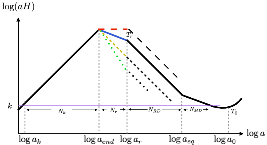
Fig. 1 shows the comoving Hubble parameter $aH$ with time Baumann:2009ds . It grows for $N_{k}$ $e$-folds during inflation with a time dependence that is fixed given a specific inflaton potential $V(\phi)$. It then decreases for $N_{\rm re}$ $e$-folds of expansion during which the energy in the inflaton potential is dissipated into a radiation bath. The standard radiation-dominated era then proceeds for $N_{\rm RD}$ $e$-folds before the advent of matter domination (and then dark-energy domination). It is clear from the Figure that the number of $e$-folds of expansion between the time that a given scale exits the horizon and the end of inflation is related to the number of $e$-folds since the end of inflation until that scale re-enters the horizon during matter/radiation-domination. The expansion history also determines the evolution of the energy density, and a second relation can be obtained from a given expansion history by demanding the proper relation between the energy density during inflation and the energy density today.

A consistent model for inflation must have an inflaton potential $V(\phi)$ that at some point steepens so that the slow-roll condition $\epsilon<1$ (where $\epsilon=(V^{\prime}/V)^{2}/2M_{\mathrm{pl}}^{2}$ is the slow-roll parameter and $M_{\mathrm{pl}}$ is the reduced Planck mass) breaks down, at which point inflation ends. The number of $e$-folds between the time that a comoving scale $k$ exits the horizon and the end of inflation is

$$N_{k}=\int_{\phi_{k}}^{\phi_{\rm end}}\,\frac{H\,d\phi}{\dot{\phi}},$$ (1)

where $\phi_{k}$ is the inflaton value when $k$ exits the horizon, $H(\phi)$ is the Hubble parameter, and the dot denotes a derivative with respect to time $t$. The Hubble parameter can then be written in terms of the inflaton potential using the Friedmann equation, $H^{2}\simeq V/(3M_{\rm pl}^{2})$, and $\dot{\phi}$ is evaluated through the slow-roll equation, $3H\dot{\phi}+V^{\prime}(\phi)\simeq 0$, where the prime denotes derivative with respect to $\phi$. The values of the scalar spectral index $n_{s}$ and tensor-to-scalar ratio $r$ can be obtained as a function of $N_{k}$. Given the relation between $N_{k}$ and the number of post-inflation $e$-folds of expansion, the value of $N_{k}$ relevant for cosmic microwave background measurements is a fixed function of $n_{s}$ once a given reheating history (specified by $w_{\mathrm{re}}$ and the reheat temperature $T_{\mathrm{re}}$) is assumed. Below we will use the fairly well-determined value of $n_{s}$ to infer, for a given reheat scenario, the inflaton-potential parameters and from them the allowable values of $r$.

Let us consider the pivot scale $k=0.05~{}{\rm Mpc}^{-1}$ at which Planck determines $n_{s}$ Ade:2013uln . The comoving Hubble scale $a_{k}H_{k}=k$ when this mode exited the horizon is related to that, $a_{0}H_{0}$, of the present time by,

$$\frac{k}{a_{0}H_{0}}=\frac{a_{k}}{a_{\rm end}}\frac{a_{\rm end}}{a_{\rm re}}\frac{a_{\rm re}}{a_{\rm eq}}\frac{a_{\rm eq}H_{\rm eq}}{a_{0}H_{0}}\frac{H_{k}}{H_{\rm eq}},$$ (2)

where quantities with subscript $k$ are evaluated at horizon exit. The other subscripts refer to the end of inflation (${\rm end}$), reheating (${\rm re}$), radiation-matter equality (${\rm eq}$), and the present time ($0$). Using $e^{N_{k}}=a_{\rm end}/a_{k}$, $e^{N_{\rm re}}=a_{\rm re}/a_{\rm end}$ and $e^{N_{\rm RD}}=a_{\rm eq}/a_{\rm re}$, we obtain the constraint,

$$\ln\frac{k}{a_{0}H_{0}}=-N_{k}-N_{\rm re}-N_{\rm RD}+\ln\frac{a_{\rm eq}H_{\rm eq}}{a_{0}H_{0}}+\ln\frac{H_{k}}{H_{\rm eq}},$$ (3)

on the total expansion Liddle:2003as . The Hubble parameter during inflation is given by $H_{k}=\pi M_{\mathrm{pl}}\left(rA_{s}\right)^{1/2}/\sqrt{2}$, with the primordial scalar amplitude $\ln(10^{10}A_{s})=3.089^{+0.024}_{-0.027}$ from Planck Ade:2013uln .

The energy density $\rho_{\mathrm{end}}$ at the end of inflation is related to the energy density $\rho_{\mathrm{re}}$ at the end of reheating by the equation-of-state parameter $w_{\mathrm{re}}$ during reheating via

$$\dfrac{\rho_{\mathrm{re}}}{\rho_{\mathrm{end}}}=\exp[-3N_{\rm re}(1+w_{\mathrm{re}})],$$ (4)

where $N_{\rm re}$ is the number of $e$-folds of expansion during reheating.

The energy density at the end of inflation is obtained from

$$\rho_{\mathrm{end}}=(1+\lambda)V_{\mathrm{end}},$$ (5)

where the ratio $\lambda$ of kinetic to potential energies at the end of inflation is

$$\lambda=\dfrac{1}{3/\epsilon-1}.$$ (6)

When inflation ends ($\epsilon\approx 1$), we have $\lambda\approx 1/2$.

We next calculate the energy density at reheating. Assuming conservation of entropy,

$$g_{\mathrm{s,re}}T_{\mathrm{re}}^{3}=\left(\dfrac{a_{0}}{a_{\mathrm{re}}}\right)^{3}\left(2T_{0}^{3}+\dfrac{21}{4}T_{\nu,0}^{3}\right),$$ (7)

where $g_{\mathrm{s,re}}$ is the effective number of relativistic degrees of freedom at reheating, and $T_{\nu,0}=(4/11)^{1/3}T_{0}$ is the current neutrino temperature. Thus,

$$\dfrac{T_{\mathrm{re}}}{T_{0}}=\left(\dfrac{43}{11g_{\mathrm{s,re}}}\right)^{1/3}\dfrac{a_{0}}{a_{\mathrm{eq}}}\dfrac{a_{\mathrm{eq}}}{a_{\mathrm{re}}}.$$ (8)

Since the energy density at reheating is $\rho_{\mathrm{re}}=(\pi^{2}g_{\mathrm{re}}/30)T_{\mathrm{re}}^{4}$, we plug Eq. (8) into Eq. (4) to get the number $N_{\rm re}$ of $e$-folds during reheating as a function of the number $N_{\rm RD}$ of $e$-folds during radiation domination. Plugging that into Eq. (3) we obtain finally,

$$N_{\rm re} = \dfrac{4}{1-3\,w_{\mathrm{re}}}\left[-N_{k}-\log(\dfrac{k}{a_{0}T_{0}})-\dfrac{1}{4}\log\left(\dfrac{30}{g_{\mathrm{re}}\pi^{2}}\right)\right.$$ (9)

$$\left.-\dfrac{1}{3}\log\left(\dfrac{11g_{\mathrm{s,re}}}{43}\right)-\dfrac{1}{4}\log\left(V_{\mathrm{end}}\right)-\right.$$

$$\left.-\dfrac{1}{4}\log(1+\lambda)+\dfrac{1}{2}\log\left(\dfrac{\pi^{2}rA_{s}}{2}\right)\right],$$

where $g_{\mathrm{re}}$ and $g_{\mathrm{s,re}}$ can be both taken to be $\approx 100$ and we will use $k=0.05\,\mbox{Mpc}^{-1}$ throughout the paper, albeit keeping the subindex $k$ in $N_{k}$ to avoid confusion. Then using Eq. (4), the reheating temperature is,

$$T_{\mathrm{re}}=\exp\left[{-\frac{3}{4}(1+w_{\mathrm{re}})N_{\rm re}}\right]\left(\dfrac{3}{10\pi^{2}}\right)^{1/4}(1+\lambda)^{1/4}V_{\mathrm{end}}^{1/4}.$$ (10)

Figure 2: In the lower panels we plot the reheat temperature $T_{\rm re}$ for natural inflation as determined by matching the number of $e$-folds during and after inflation. Results are shown for decay constants $f=5\,M_{\mathrm{pl}}$, 7 $M_{\mathrm{pl}}$, and $\infty$, where the latter corresponds to the $m^{2}\phi^{2}$ limit. Four different effective equation-of-state parameters $w_{\mathrm{re}}$ for reheating are considered in each case: from left to right in their intersection with the bottom of the plots they are $w_{\mathrm{re}}=-1/3$ (red), $w_{\mathrm{re}}=0$ (blue), $w_{\mathrm{re}}=0.25$ (black), and $w_{\mathrm{re}}=1$ (green). The values $w_{\mathrm{re}}=-1/3$ and $w_{\mathrm{re}}=1$ bracket the very most conservative allowed range of values for $w_{\mathrm{re}}$, while $w_{\mathrm{re}}=0$ and $w_{\mathrm{re}}=0.25$ bracket the range suggested by the literature on reheating. All curves intersect at the point where reheating occurs instantaneously, and the $w_{\mathrm{re}}=1/3$ curve would be vertical. Values of the termination condition in the range $0.1\lesssim\epsilon\lesssim 1$ give rise to variations that are narrower than the widths of the curves. The light purple regions are below the electroweak scale $T_{\rm EW}\sim 100~{}{\rm GeV}$. The dark purple regions, below $10~{}{\rm MeV}$, would ruin the predictions of big bang nucleosynthesis (BBN). Temperatures above the intersection point are unphysical as they correspond to $N_{\rm re}<0$. The gray shaded triangles indicate the parameter space allowed if $0<w_{\mathrm{re}}<0.25$. The light yellow band indicates the $1\sigma$ range in $n_{s}-1=-0.0397\pm 0.0073$ from Planck Ade:2013uln , and the dark yellow band assumes a projected uncertainty of $10^{-3}$ 1404.1065 for $n_{s}-1$ as expected from future experiments (assuming the central value remains unchanged). The top panels plot the number $N_{k}$ of $e$-folds of inflation as a function of $n_{s}$. The vertical dashed red lines demarcate the allowed range of $n_{s}$, inferred from the lower panel, and the horizontal dashed red lines in the upper panels indicate the allowed range of values of $N_{k}$.

III Inflaton potentials

We now discuss the two classes of inflation models that we consider in this work.

III.1 Natural Inflation

This model, first proposed in Ref. Adams:1992bn , appears when a global $U(1)$ symmetry is spontaneously broken. The inflaton is then the pseudo-Nambu-Goldstone boson. The shift symmetry protects the flatness of the potential. The inflaton potentials we consider are,

$$V(\phi)=\dfrac{2\Lambda^{4}}{2^{m}}\left(1+\cos\phi/f\right)^{m},$$ (11)

where the energy density $\Lambda^{4}$ and decay constant $f$ are the parameters of the model. We generalize the usual natural-inflation potential, which has $m=1$, to other values of $m$ to broaden slightly the class of models we consider. The slow-roll parameters for this model are

$$\epsilon=m^{2}\dfrac{e^{-x}}{2f^{2}(1-e^{-x})+m},\qquad\mbox{where}\quad x=\dfrac{mN_{k}}{f^{2}},$$ (12)

and

$$\eta=\eta_{V}-\epsilon=\dfrac{-m}{2f^{2}}\,\dfrac{2f^{2}(1-me^{-x})+m}{2f^{2}(1-e^{-x})+m}.$$ (13)

These lead to the observables $r$ and $n_{s}-1$, which are

$$r=8m^{2}\dfrac{e^{-x}}{2f^{2}(1-e^{-x})+m},$$ (14)

and

$$n_{s}-1=-\dfrac{m}{f^{2}}-\dfrac{2m(m+1)\,e^{-x}}{2f^{2}(1-e^{-x})+m}.$$ (15)

We will also need to calculate the number $N_{k}$ of $e$-folds that happen after a mode with wavenumber $k$ exits the horizon, which is found to be

$$N_{k}=\dfrac{f^{2}}{m}\log\left[\dfrac{1}{1+m/(2f^{2})}\dfrac{(n_{s}-1)f^{2}-m^{2}}{(n_{s}-1)f^{2}+m}\right].$$ (16)

Even though the model has two parameters ($\Lambda$ and $f$) only one of them is free, since they are related through the amplitude of the scalar power spectrum. From the value of the potential $V_{k}$ at horizon exit we find $\Lambda$ to be,

$$\Lambda=\left(\dfrac{3}{4}\pi^{2}rA_{s}\left[\dfrac{2f^{2}+n}{2f^{2}(1-e^{-mN_{k}/f^{2}})+m}\right]^{m}\right)^{1/4}.$$ (17)

In the $f\to\infty$ limit these potentials behave like pure power laws; i.e.,

$$V(\phi)\sim M^{4-2m}\phi^{2m}\quad\mbox{when}\quad f\to\infty,$$ (18)

where $M$ is an energy scale that plays the role of $\Lambda$ and is also fixed.

III.2 Higgs-like Inflation

The potentials we consider for Higgs-like inflation are,

$$V(\phi)=\Lambda^{4}\left[1-(\phi/\mu)^{2}\right]^{n},$$ (19)

with slow-roll parameters,

$$\epsilon=\frac{2n^{2}y}{\mu^{2}(1-y)^{2}},$$ (20)

and

$$\eta=\eta_{V}-\epsilon=\frac{2n[-1+(n-1)y]}{\mu^{2}(1-y)^{2}}.$$ (21)

The variable $y$ is defined as,

$$y(\mu)\equiv\phi_{0}^{2}/\mu^{2}=-W\left(-g(\mu)\exp\left[{-g(\mu)-\frac{8N_{k}}{\mu^{2}}}\right]\right),$$ (22)

where $W(z)$ is the Lambert $W$ function, and

$$g(\mu)\equiv\left(\phi_{\mathrm{end}}/\mu\right)^{2}=1+\dfrac{n^{2}}{\mu^{2}}-\dfrac{\sqrt{n^{4}+2\mu^{2}n^{2}}}{\mu^{2}}<1.$$ (23)

Again, we generalize the usual case ($n=2$) to explore a broader class of models. In the general case the tensor-to-scalar ratio and scalar spectral index are,

$$r=\frac{16n^{2}y}{\mu^{2}(1-y)^{2}},$$ (24)

and

$$n_{s}-1=-\dfrac{4n}{f^{2}}\dfrac{[1+(n+1)y]}{(1-y)^{2}}.$$ (25)

We will again need the number,

$$N_{k}=\frac{\mu^{2}}{4n}\left[-\log\left(\frac{y}{g}\right)+y-g\right],$$ (26)

of $e$-folds of inflation, and once again we can express the amplitude $\Lambda$ of the potential in terms of the scalar power-spectrum amplitude $A_{s}$ and the decay constant $\mu$,

$$\Lambda=\left[\dfrac{3}{2}\pi^{2}rA_{s}\left(1-y\right)^{-n}\right]^{1/4}.$$ (27)

This model also behaves as a power law in the $\mu\to\infty$ limit, the exponent being in this case $n$,

$$V(\phi)\sim M^{4-n}\phi^{n}\quad\mbox{when}\quad\mu\to\infty.$$ (28)

IV Results

Figure 3: Same as Fig. 2 but for Higgs-like inflation with parameter values $\mu=14\,M_{\mathrm{pl}}$, 20 $M_{\mathrm{pl}}$, and $\infty$.

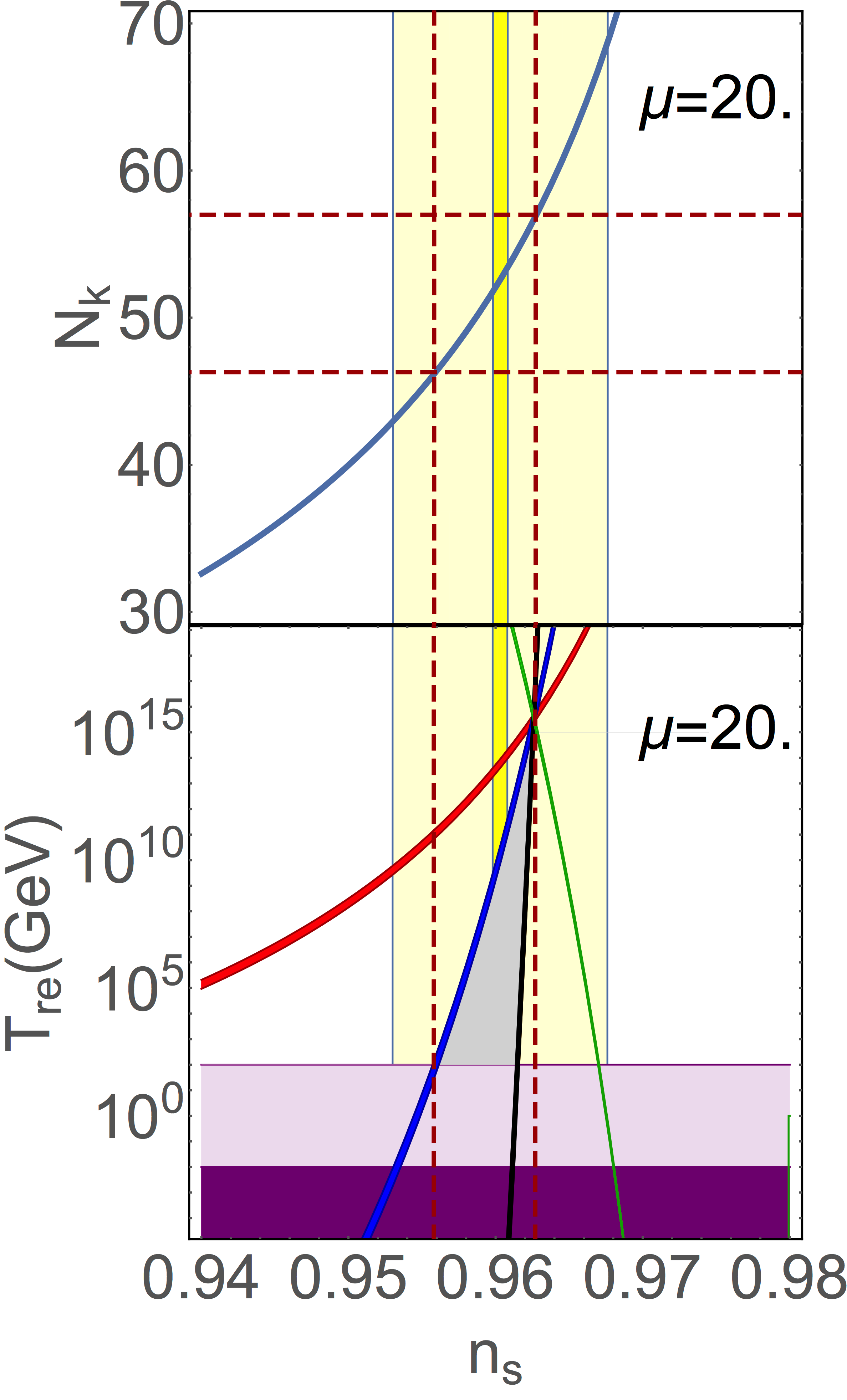
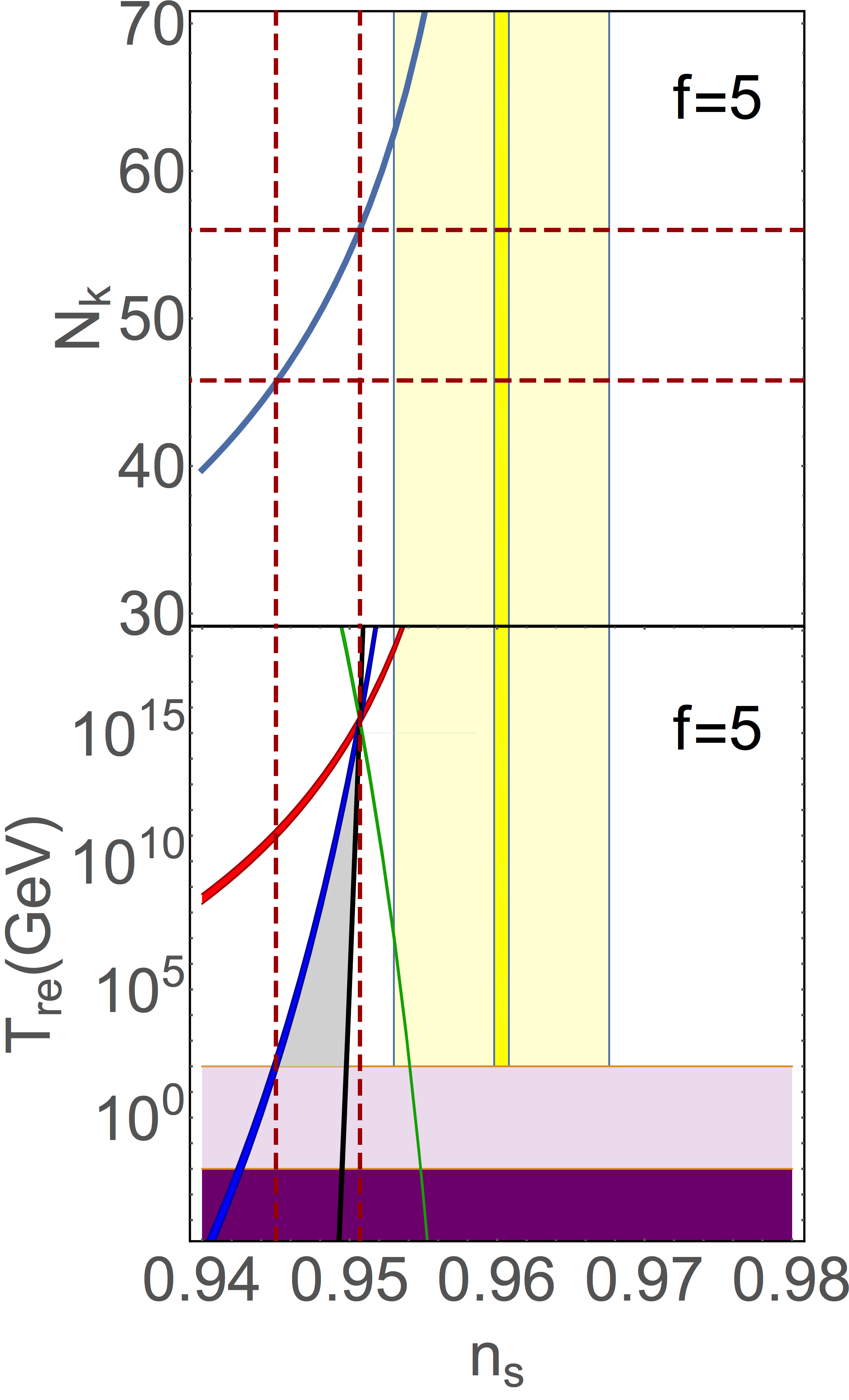
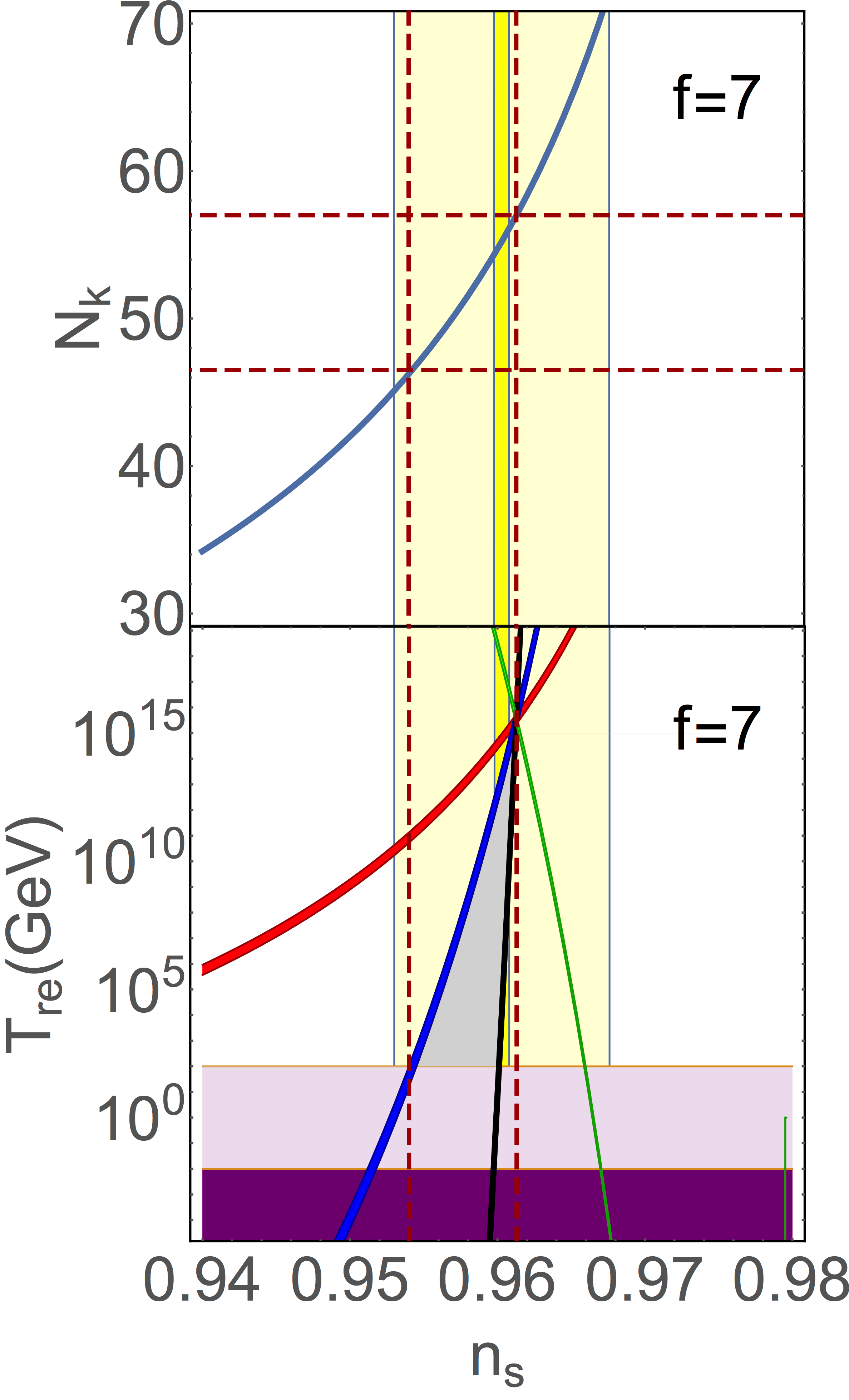
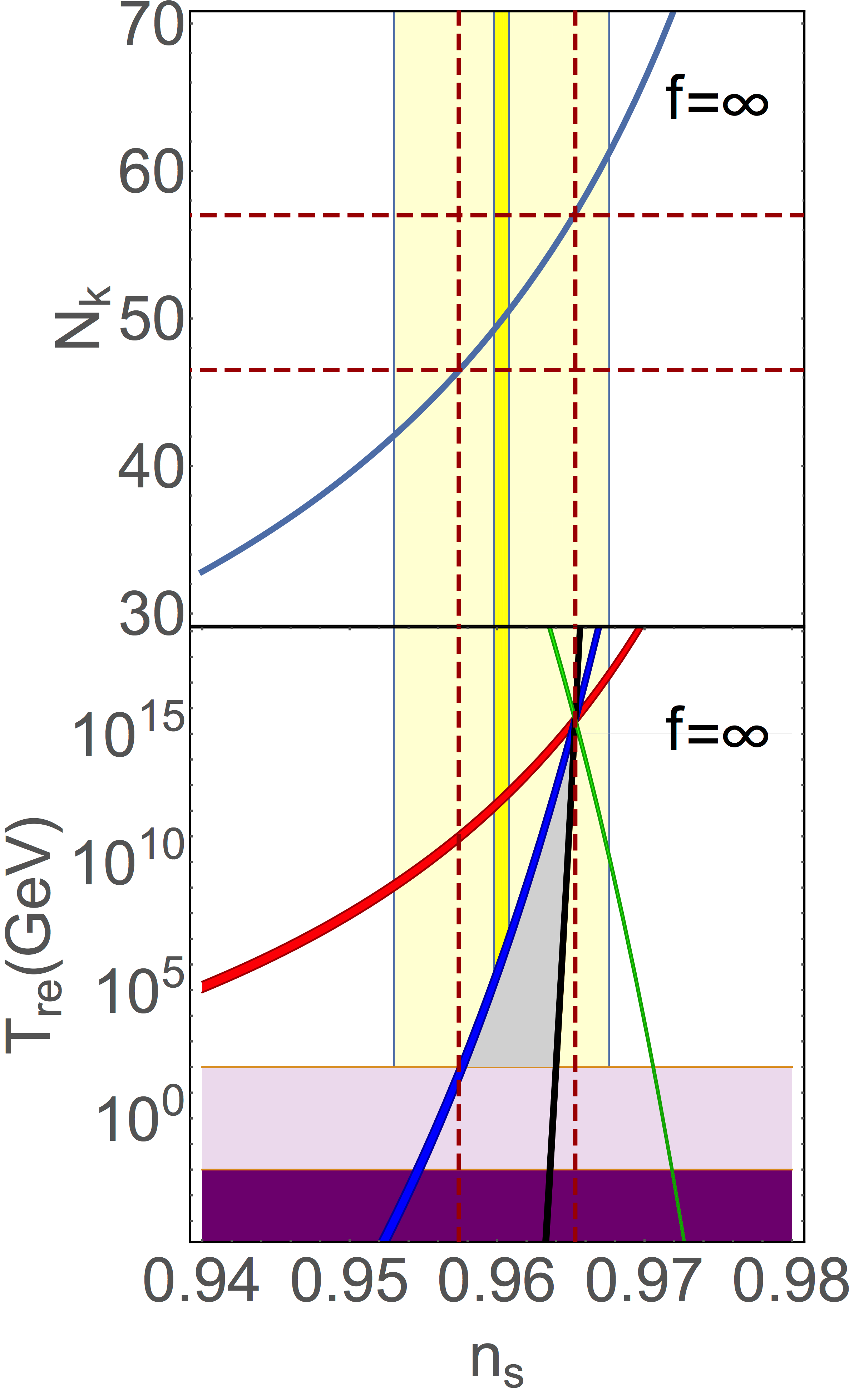
The results of the calculation are shown for usual natural inflation in Fig. 2 and for usual Higgs-like inflation in Fig. 3. The reheat temperature $T_{\rm re}$ determined by matching the number of $e$-folds during and after inflation is shown in the lower panels of each Figure. We show results for four different reheating effective equation-of-state parameters $w_{\mathrm{re}}$. The value $w_{\mathrm{re}}=-1/3$ indicates the smallest possible value of $w_{\mathrm{re}}$ required for inflation to end. The value $w_{\mathrm{re}}=1$ provides the most conservative upper limit which comes simply from causality. The values $w_{\mathrm{re}}=0$ and $w_{\mathrm{re}}=0.25$ bracket the range of values of $w_{\mathrm{re}}$ in detailed models of reheating. The curves for all values of $w_{\mathrm{re}}$ intersect at the point where reheating is instantaneous, and the $w_{\mathrm{re}}=1/3$ curve would be vertical and intersect this point. The gray shaded triangles indicate the region allowed if the reheating equation-of-state parameter lies in the range $0<w_{\mathrm{re}}<0.25$.

The top panels of Figs. 2 and 3 plot the number $N_{k}$ of $e$-folds during inflation for each model and value of $f$ (for natural inflation) or $\mu$ (for Higgs-like inflation). It can be seen, in particular, that the limit to the allowable range of values of $n_{s}$ imposed by reheating considerations thus restricts the allowed range of values of $N_{k}$. The range of values of $N_{k}$ is generally smaller than the range $N_{k}\simeq 46-60$ often assumed, being replaced (at our pivot scale $k=0.05$ Mpc^-1) by $N_{k}\simeq 47-57$ for the large $f,\,\mu$ limit, and slightly smaller values for lower $f,\,\mu$.

It is also important to note that the tightness of the constraint to the $n_{s}$ parameter space for fixed $f$ (for natural inflation) or $\mu$ (for Higgs-like inflation) is determined not by the precision of current measurements, but by the self consistency of the inflationary-plus-reheating model. For the $m^{2}\phi^{2}$ case the new range of possible $n_{s}$ for inflation is (0.958,0.965).

Figure 4: The $n_{s}$-$r$ parameter space for (left) natural inflation and (right) Higgs-like inflation. Curves that indicate instantaneous reheating (red) and reheating at the electroweak scale (black) are shown as well as curves that show $N_{k}=46$ and $N_{k}=60$ $e$-folds of reheating (purple). Diagonal blue lines indicate different values of the decay constants $f$ or $\mu$, where the orange line is the power-law limit. The horizontal dotted lines indicate the smallest tensor-to-scalar ratio $r$ consistent with the $1\sigma$ range of values of the scalar spectral index $n_{s}$, obtained by restricting the reheating equation-of-state parameter to physically plausible values, which are higher by about 25$\%$ than those obtained by simply taking a range $N_{k}=46-60$ for the number of $e$-folds of reheating.

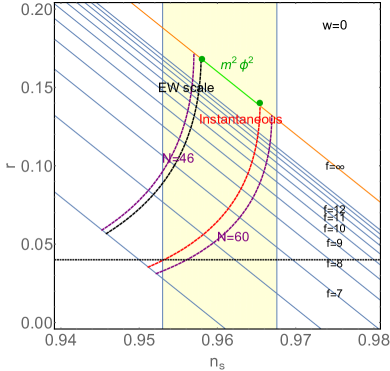
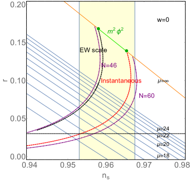
We also show results in Fig. 4 as plots of the $r$-$n_{s}$ parameter space for natural inflation and for Higgs-like inflation. It is seen here that even after considering the complete range of values of $f$ (for natural inflation) or $\mu$ (for Higgs-like inflation), the parameter space allowed by restricting the reheating equation-of-state parameter to physically plausible values is more constrained than that assumed simply taking a range $N_{k}=46-60$ for the number of $e$-folds of inflation. In particular, we see that the smallest tensor-to-scalar ratio $r$ allowed by the current $1\sigma$ range of values for $n_{s}$ is a bit larger with our approach than that obtained with the less restrictive analysis. The black (dashed) curves correspond to the maximum reheating possible with equation-of-state parameter $w_{\mathrm{re}}=0$. Increasing the value of $w_{\mathrm{re}}$ would only shift the black curves to the right.

V Conclusions

We have explored a new technique to find constraints to inflationary models by studying their reheating period. Instead of focusing on the physics of the reheating phase itself, or assuming an overly ample parameter space by constraining the number of $e$-folds of inflation, we characterize the whole reheating era by a single equation-of-state parameter $w_{\mathrm{re}}$, that we constrain to have physically reasonable values. This leads to more precise constraints to the inflationary observables.

We have applied this formalism to two families of potentials (natural inflation and Higgs-like inflation), finding better lower bounds for the tensor-to-scalar ratio $r$, as can be seen in Table 1 (where the usual $m=1$, $n=2$ potentials are in bold face). It is important to notice that these results are robust to changes in the equation-of-state parameter as long as it is kept under $w_{\mathrm{re}}=$1/3, as suggested by the literature on reheating.

The results derived for the potentials studied also apply, taking the limiting cases $f$ or $\mu\to\infty$, to power-law models and, as we show in Figure 4, the allowed region for the power-law case (green line) is more constrained using our method than with the usual analysis in which the range for the numbers of $e$-folds is fixed. For comparison, the right-hand plots in Figures 2 and 3 correspond to the plot made on Dai:2014jja for $m^{2}\phi^{2}$ potential, showing in the upper panel $N_{k}$ instead of $N_{\rm re}$.

Model	$r_{\mathrm{m}in}$ old	$r_{\mathrm{m}in}$ new
Higgs $n=1$	0.020	0.025
Higgs $\mathbf{n}=$ 2	0.024	0.030
Higgs $n=3$	0.035	0.050
Higgs $n=4$	0.055	0.070
Natural $\mathbf{m}=$ 1	0.033	0.040
Natural $m=3/2$	0.055	0.070
Natural $m=2$	0.10	not allowed
$m^{2}\phi^{2}$	0.13	0.14

Table 1: Minimum value of the tensor-to-scalar ratio $r$ at the pivot scale $k=0.05$ Mpc^-1 allowed by reheating considerations and the Planck $1\sigma$ range of values of the scalar spectral index $n_{s}$ for each of the models studied. In the central column we show the minimum $r$ from the usual analysis in which a range of $N_{k}$ is allowed, and in the right column the new minimum obtained by constraining the reheating equation-of-state.

The most interesting feature of this technique is its general validity. It was considered for power-law potentials in Refs. Dai:2014jja ; Creminelli:2014fca , and we have generalized here to natural and Higgs-like potentials. Still, the approach can be similarly applied to any single-field inflation model and will generically lead to slightly more restrictive bounds to the inflationary parameter space, including the range of values of the tensor-to-scalar ratio $r$. As a result, upper bounds to $r$, for example, will generally be slightly more restrictive to inflationary models than they would otherwise be.