Vortex Nucleation in a Dissipative Variant of the Nonlinear Schrödinger Equation under Rotation

Abstract

In the present work, we motivate and explore the dynamics of a dissipative variant of the nonlinear Schrödinger equation under the impact of external rotation. As in the well established Hamiltonian case, the rotation gives rise to the formation of vortices. We show, however, that the most unstable mode leading to this instability scales with an appropriate power of the chemical potential $\mu$ of the system, increasing proportionally to $\mu^{2/3}$. The precise form of the relevant formula, obtained through our asymptotic analysis, provides the most unstable mode as a function of the atomic density and the trap strength. We show how these unstable modes typically nucleate a large number of vortices in the periphery of the atomic cloud. However, through a pattern selection mechanism, prompted by symmetry-breaking, only few isolated vortices are pulled in sequentially from the periphery towards the bulk of the cloud resulting in highly symmetric stable vortex configurations with far fewer vortices than the original unstable mode. These results may be of relevance to the experimentally tractable realm of finite temperature atomic condensates.

mmsxxxxxxxx–x

1 Introduction

Vortices are persistent circulating flow patterns that occur in many diverse scientific and mathematical contexts [1], ranging from hydrodynamics, superfluids, and nonlinear optics [2, 3] to specific case examples in sunspots, dust devils [4], and plant propulsion [5]. The realm of atomic Bose-Einstein condensates (BECs) [6, 7, 8] has produced a novel and pristine setting where numerous features of the exciting nonlinear dynamics of single- and multi-charge vortices, as well as of vortex crystals and vortex lattices, can be not only theoretically studied, but also experimentally observed.

The first experimental observation of vortices in atomic BECs [9] by means of a phase-imprinting method between two hyperfine spin states of a ⁸⁷Rb BEC [10] paved the way for a systematic investigation of their dynamical properties. Stirring the BECs [11] above a certain critical angular speed [12, 13, 14] led to the production of few vortices [14] and even of robust vortex lattices [15, 16]. Other vortex-generation techniques were also used in experiments, including the breakup of the BEC superfluidity by dragging obstacles through the condensate [17], as well as nonlinear interference between condensate fragments [18]. In addition, apart from unit-charged vortices, higher-charged vortex structures were produced [19] and their dynamical (in)stability was examined. To these earlier experimental developments, one can add in recent years: the formation of vortices through a quench of a gas of atoms from well above to well-below the BEC transition via the so-called Kibble-Zurek mechanism [20]; the dynamical visualization of such “nucleated” vortices [21] and even of vortex pairs, i.e., dipoles consisting of two oppositely charged vortices; the nucleation of dipoles via the dragging of a laser beam through the BEC [22]; the systematic experimental exploration of dipole dynamics [23]; the generation (via instabilities) of 3-vortex configurations of same or opposite signs in Ref. [24] and the “dialing in” of arbitrary numbers of (few) same-charge vortices and the visualization of their intriguing, potentially symmetry-breaking dynamics [25]. Naturally, the above developments suggest that the study of vortices and of their nucleation in BECs is a theme of broad and intense ongoing interest.

On the other hand, another topic receiving increasing attention has concerned the role of finite-temperature induced “damping” of the BEC [26]. A wide range of recent examples has indicated that this leads to anti-damping motion of the coherent structures such as solitary waves (dark solitons) and vortices. Early soliton experiments of about 15 years ago observed the motion of a dark soliton towards the edge of the trap [27, 28, 29]. It is interesting to note, however, that this type of anti-damping effect has been observed in a far more pronounced way in recent experiments of dark soliton oscillations in a unitary Fermi gas [30]. A number of theoretical studies have provided relevant explanation for this phenomenology in atomic BECs [31, 32, 33, 34, 35, 36, 37, 38, 39]. In particular, it has been identified in these works that the dark soliton follows an anti-damped harmonic oscillator behavior, leading to trajectories of growing amplitude around the center of the trap, until expelled from the BEC. This motion has been observed in the context of the so-called dissipative Gross-Pitaevskii equation model (DGPE). The DGPE was originally introduced phenomenologically by Pitaevskii [40] as a way to use a damping term to account for the role of finite temperature induced fluctuations in the BEC dynamics; see, e.g., Refs. [41, 42, 43, 44] for discussions and microscopic interpretations of such a term. Comparisons [33] of its results with more elaborate models such as the (averaged quantities of) the stochastic Gross-Pitaevskii equation (SGPE) [45, 46] offered good reason for exploring the simpler DGPE model, as regards coherent structure (such as soliton) dynamics.

More importantly for our theme of vortex dynamics, an increasing volume of literature has been exploring the role of thermal effects [47, 48, 49, 50, 51]. Here, too, and in accordance with theoretical predictions [52] (see also Ref. [53] and for a recent discussion [54]), an outward, in this case spiraling, trajectory is found for the single vortex motion which leads to its expulsion from the trap. While important aspects of the vortex dynamics in the presence of the thermal component such as the single vortex motion [52, 53] and even the vortex-pair interaction [54] have been explored theoretically (and numerically), to the best of our knowledge, the predictions of the DGPE model in the context of vortex nucleation under rotation have not been previously examined.

The principal scope of our study will, thus, be to provide some insight on the instability and dynamics that leads to the emergence of vortices in the presence of “thermal dissipation”, i.e., in the DGPE framework. In fact, to facilitate the analysis, we will go one step further in simplifying the problem and will also explore the “imaginary time” analogue of the GPE. This choice will be suitably explained and motivated in the next section. Subsequently, in Section 3, we will provide the analysis that identifies the most unstable eigenmode and its scaling with the system parameters (most notably, the chemical potential $\mu$). Finally, in Section 4, we will summarize our findings and present a number of directions for future study.

2 Model Setup: the NLS Equation Under Rotation and its Dissipative Variant

2.1 Dissipationless case

The standard GPE model valid at $T=0$ for describing the the quasi-2D condensate wavefunction $u(x,y,t)$ in the presence of rotation is:

$$iu_{t}=-\frac{1}{2}\Delta u+\frac{1}{2}\Omega_{\rm trap}^{2}r^{2}u-\mu u+|u|^{2}u+i\Omega_{\rm rot}u_{\theta},$$ (1)

where $(\cdot)_{t}=d(\cdot)/dt$ and $(\cdot)_{\theta}=d(\cdot)/d\theta$ and $(r,\theta)$ are the polar coordinates. Here the potential is assumed as representing a parabolic (typically induced magnetically) trap of strength $\Omega_{\rm trap}$, while an external rotation of strength $\Omega_{\rm rot}$ is assumed to be imposed. We have also explicitly included the chemical potential $\mu$ in the model (although it can be factored out by a gauge transformation), as it will be relevant in the DGPE variant of the system. Notice that here we use the dimensionless form of the pancake-shaped, 2D BEC model that has been well established in a variety of archival references in the field [7, 8, 55].

Before we move to the DGPE variant of the model, we should note a remarkable implication of Eq. (1). In particular, when analyzing the spectrum of a particular state $u_{0}$, by performing Bogolyubov-de Gennes (BdG) analysis to explore its stability, the equation obtained for $u=u_{0}(x,y)+\epsilon v(x,y,t)$ is of the form:

$$iv_{t}=-\frac{1}{2}\Delta v+\frac{1}{2}\Omega_{\rm trap}^{2}r^{2}v-\mu v+2|u_{0}|^{2}v+u_{0}^{2}v^{\star}+i\Omega_{\rm rot}v_{\theta},$$ (2)

where $(\cdot)^{\star}$ denotes complex conjugation. Now, decomposing the perturbation as $v(x,y,t)=a(r)e^{im\theta}e^{i\omega t}+b(r)e^{-im\theta}e^{-i\omega t}$, it is straightforward to see that for a radial state (such as the ground state of the system), the sole influence of the rotation frequency $\Omega_{\rm rot}$ is to shift the frequencies $\omega\rightarrow\omega\pm m\Omega_{\rm rot}$.

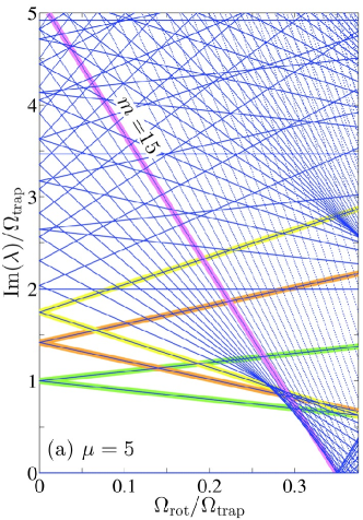
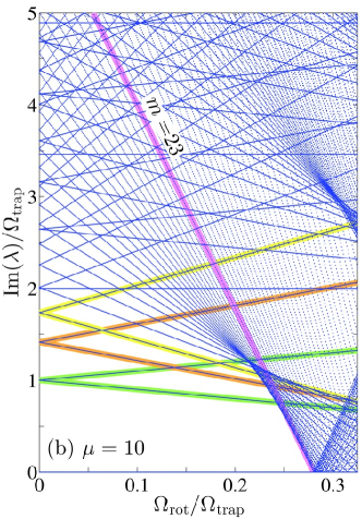
Fig. 1: (color online) The spectrum of imaginary eigenvalues (normalized to the trap frequency) of the Hamiltonian linearization problem of Eq. (2) in the presence of rotation. The left panel is for $\mu=5$, while the right one is for $\mu=10$; $\Omega_{\rm trap}=0.2$ was chosen. The thick green, orange and yellow lines correspond to the lowest three modes of $m=1,2,3$, giving the theoretical prediction of how they depend as a function of frequency according to $\lambda=i(\omega(m=0)\pm m\Omega_{\rm rot})$. The thick pink line corresponds to the $m=m_{c}$ mode that first becomes unstable as the rotation is increased. $m_{c}=15$ for $\mu=5$ and $m_{c}=23$ for $\mu=10$.

This is illustrated, e.g., in Fig. 1 by direct numerical computations involving the BdG linearization around the ground state for the case of $\Omega_{\rm trap}=0.2$ for 2 different values of $\mu=5$ (left) and $\mu=10$ (right). The lowest, well-known modes of the condensate dynamics namely the dipolar, quadrupolar, and hexapolar modes at, respectively, $\omega=\Omega_{\rm trap}$, $\omega=\sqrt{2}\Omega_{\rm trap}$, and $\omega=\sqrt{3}\Omega_{\rm trap}$ (all with double degeneracy), are shown by thick green, orange and yellow lines respectively, showcasing the validity of the above eigenfrequency shift statement. However, there are numerous additional intriguing features to observe in the figure. For one thing, we note that since the ground state is stable and its imaginary eigenvalues (real eigenfrequencies) shift along the imaginary axis of the complex spectral plane (Re($\lambda$),Im($\lambda$)), the ground state will never become dynamically unstable. Instead, what happens is that it becomes energetically unstable acquiring what is known as negative energy modes [56] or in the mathematical literature as negative Krein signature modes [57]. These modes indicate that while the solution may not be dynamically unstable, it is no longer the ground state of the system. Moreover, if a pathway, such as the presence of dissipation, becomes available for relaxing to the ground state of the system then it would do so [58].

Some additional observations are also in order. In particular, it is worthwhile to note that among the modes crossing zero to become negative energy or signature ones, it is neither the $m=1$, nor the $m=2$ ones that do this the first. Instead, modes associated with higher $m$ (but which start at larger $\omega$) values move faster and cross $0$, spearheading the energetic instability of the present state. For instance, as is depicted in Fig. 1, the modes with $m=m_{c}=15$ and $m=m_{c}=23$ are the first modes to cross the energetic stability threshold for, respectively, $\mu=5$ and $\mu=10$. This instability occurs at $\Omega_{\rm rot}=\Omega_{{\rm rot},c}\approx 0.349\,\Omega_{\rm trap}$ for $\mu=10$ and at $\Omega_{\rm rot}=\Omega_{{\rm rot},c}\approx 0.28\,\Omega_{\rm trap}$ for $\mu=5$. Notice that the critical rotation threshold for $\mu=5$ is larger that the one for $\mu=10$, an important feature to which we will return below. The reason why the above observations are especially interesting is the following. As proved rigorously in Ref. [57], the inclusion of dissipation in a Hamiltonian model leads modes of different energy (Krein signature) to move differently, due to their distinct topological characteristics. More specifically, modes with positive signature move to the left of the spectral plane becoming stable/attracting eigendirections for the dynamics. However, modes with negative Krein signature move in the opposite direction of the spectral plane, namely to the right hand plane, becoming immediately unstable as soon as the dissipation is turned on. This statement goes hand-in-hand with the opening of relaxation channels through which the solution can now revert to its preferred ground state equilibrium, given its energetic instability.

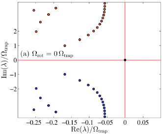
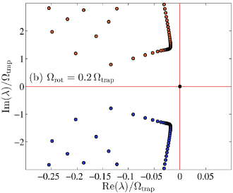
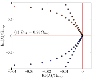
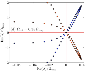
Fig. 2: (color online) Spectral planes increasing rotation: (a) $\Omega_{\rm rot}=0$, (b) $\Omega_{\rm rot}/\Omega_{\rm trap}=0.2$, (c) $\Omega_{\rm rot}/\Omega_{\rm trap}=0.28$ and (d) $\Omega_{\rm rot}/\Omega_{\rm trap}=0.35$, all for $\gamma=0.01$ and $\mu=10$. Eigenvalues with positive and negative Krein sign are depicted, respectively, with blue (dark) and orange (light) points and zero-Krein eigenvalues are depicted with black points. The successive panels clearly illustrate the instability due to the collision of opposite Krein signature modes that starts at $\Omega_{{\rm rot},c}=0.28\,\Omega_{\rm trap}$ [see panel (c)].

2.2 Dissipative Gross-Pitaevskii Equation

Now, let us project the above conclusions to the case of the DGPE which is of the form [40]:

$$(i-\gamma)u_{t}=-\frac{1}{2}\Delta u+\frac{1}{2}\Omega_{\rm trap}^{2}r^{2}u-\mu u+|u|^{2}u+i\Omega_{\rm rot}u_{\theta},$$ (3)

where $\gamma$ ($>0$) refers to the temperature dependent parameter that has been discussed extensively in this context [26, 41, 42, 43, 44]. Exploring a nearly realistic (although slightly higher than relevant, for illustration purposes; see, e.g., the discussion of Ref. [54]) value of $\gamma=0.01$, we obtain the results for $\mu=10$ illustrated in Figs. 2 and 3. The former one shows the spectral planes for 4 values of the ratio $\Omega_{\rm rot}/\Omega_{\rm trap}$, two below, one (approximately) at, and one above the energetic instability threshold of the ground state. In the presence of the $\gamma$ term (irrespectively of however small), when all the modes are positive energy ones, i.e., below the threshold of $\Omega_{{\rm rot},c}=0.28\,\Omega_{\rm trap}$, all of the eigenvalues are on the left half plane [see Figs. 2(a) and (b)], hence the configuration is dynamically stable as well (in the DGPE case). However, above the energetic instability threshold for the Hamiltonian problem, the existence of negative Krein signature modes immediately leads to the bifurcation of unstable eigenmodes in the right half of the spectral plane [see Fig. 2(d)] and the configuration is dynamically unstable for the DGPE. This instability is manifested as a function of $\Omega_{\rm rot}/\Omega_{\rm trap}$ for the DGPE case in Fig. 3 showcasing that the nontrivial real parts of the relevant eigenvalues emerge as the threshold is crossed. To complement the instability picture, we depict in Fig. 4 the most unstable modes for rotations just above the instability threshold. For $\mu=5$ [see Fig. 4(a)] the most unstable eigenfunction for $\Omega_{\rm rot}/\Omega_{\rm trap}=0.3495$ (i.e., just above the threshold $\Omega_{{\rm rot},c}/\Omega_{\rm trap}\approx 0.349$) is the mode with $m=15$ as expected from Fig. 1. Similarly, for $\mu=10$ [see Fig. 4(b)], the most unstable eigenfunction for $\Omega_{\rm rot}/\Omega_{\rm trap}=0.2802$ (i.e., just above the threshold $\Omega_{{\rm rot},c}/\Omega_{\rm trap}\approx 0.28$) is the mode with $m=23$ as expected from Fig. 1.

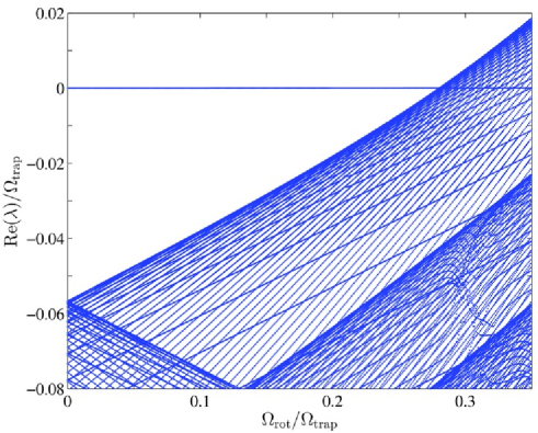
Fig. 3: (color online) The largest eigenvalues leading to the instability beyond the critical value of $\Omega_{\rm rot}/\Omega_{\rm trap}$, in the DGPE case with $\gamma=0.01$.

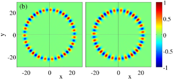
Fig. 4: (color online) The most unstable eigenfunction just past the rotation threshold. The left and right subpanels corresponds, respectively, to the real and imaginary parts of the most unstable eigenfunction. (a) For $\mu=5$ and $\Omega_{\rm rot}/\Omega_{\rm trap}=0.3495>\Omega_{{\rm rot},c}/\Omega_{\rm trap}\approx 0.349$ the most unstable eigenfunction corresponds to $m=15$. (b) For $\mu=10$ and $\Omega_{\rm rot}/\Omega_{\rm trap}=0.2802>\Omega_{{\rm rot},c}/\Omega_{\rm trap}\approx 0.28$ the most unstable eigenfunction corresponds to $m=23$.

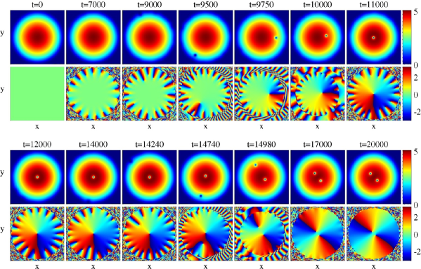
Fig. 5: (color online) Evolution of an initial steady state without vortices under rotation. The parameters are $\mu=5$, $\gamma=0.01$, $\Omega_{\rm trap}=0.2$, and $\Omega_{\rm rot}/\Omega=0.37$. For each of the times indicated, we depict the density (top sub-rows) and phase (bottom sub-rows). The windows for density and phase are, respectively, $(x,y)\in[-16,16]\times[-16,16]$ and $(x,y)\in[-29.5,29.5]\times[-29.5,29.5]$. We invite the interested reader to see the full movie at this address: http:$\mathbin{/\mkern-4.0mu/}$nonlinear.sdsu.edu/ carreter/RotatingBEC.html [Movie#1].

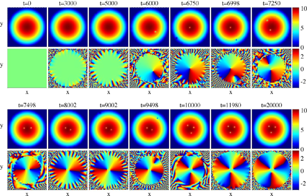
Fig. 6: (color online) Same as in Fig. 5 for $\Omega_{\rm rot}/\Omega_{\rm trap}=0.3$ and $\mu=10$. The windows for density and phase are, respectively, $(x,y)\in[-22.5,22.5]\times[-22.5,22.5]$ and $(x,y)\in[-35.8,35.8]\times[-35.8,35.8]$. We invite the interested reader to see the full movie at this address: http:$\mathbin{/\mkern-4.0mu/}$nonlinear.sdsu.edu/ carreter/RotatingBEC.html [Movie#2].

The above stability considerations allow us to understand the bifurcations (instabilities) of steady states bearing no initial vorticity as the rotation of the BEC cloud is increased. In particular, a number $N_{v}$ of vortices will be nucleated at the periphery of the cloud through an unstable eigenfunction invariant under rotations by $2\pi/N_{v}$. See for example the eigenfunctions depicted in Fig. 4. However, it is crucial to note that this analysis only captures the initial stages of the dynamical evolution and the eventual asymptotic behavior may well be different. This can be due to symmetry-breaking effects generated by infinitesimally small, non-symmetric, perturbations that will generically be present in physical (and numerical) setups. Therefore, we now explore the dynamics of the above mentioned unstable modes towards understanding what they actually nucleate as the instability sets in. For this purpose we have produced long-term simulations of the DGPE (3) starting from the stationary state bearing no vorticity. Two typical evolutions are depicted in Figs. 5 and 6 for, respectively, $\mu=5$ and $\mu=10$. We invite the interested reader to see the full movies at this address: http:$\mathbin{/\mkern-4.0mu/}$nonlinear.sdsu.edu/ carreter/RotatingBEC.html [Movies#1 and #2]. The simulations were chosen for rotations that are slightly above critical so that the steady state with no vortices is (weakly) unstable. Let us describe in detail the full evolution for the first case with $\mu=5$ for $\Omega_{\rm rot}=0.37\,\Omega_{\rm trap}>\Omega_{{\rm rot},c}\approx 0.349\,\Omega_{\rm trap}$ that is depicted in Fig. 5. As it is clear from the figure, for the chosen parameter values, the steady state with no vortices is unstable towards a mode with $m=17$ vortices initially growing at the periphery of the cloud (see snapshot at $t=7,000$). This mode is not apparent in the density distribution since it is outside the Thomas-Fermi radius where the density is too low to be able to be picked up. However, the phase distribution clearly shows a series of $2\pi$ windings that are nucleated at the periphery. It is clear that the growth of this unstable mode is prone to asymmetries since it is generated numerically from the noise inherent in the computation due to its finite precision. This effect would be similar in the physical experiments where small variations in the initial density and the trapping break the symmetry of the solution. This asymmetry is responsible for one of the vortices to be closer to the center of the cloud than its siblings. This selection mechanism is responsible for one of the vortices to start spiralling inwards (see snapshots $t=9,000$–$11,000$). It is interesting that, as the chosen vortex rotates close to its siblings, it “pushes” the other vortices outwards and thus further contributes to this selection mechanism. After the chosen vortex relaxes at the center of the trap, another unstable mode at the periphery grows and, by the same selection mechanism explained above, spirals inwards (see snapshots at $t=12,000$–$17,980$). Then, the two central vortices arrange themselves into a steady state configuration (see snapshot at $t=17,000$) with a small perturbation that remains at the periphery. However, in this case, this state is no longer unstable and hence the dynamics is eventually attracted to it (see snapshots at $t=17,000$–$20,000$). In fact, the resulting state with two corotating vortices in completely stable and thus the configuration relaxes towards it and remains there.

A similar evolution is observed in the case of $\mu=10$ and $\Omega_{\rm rot}=0.3\,\Omega_{\rm trap}>\Omega_{{\rm rot},c}\approx 0.28\,\Omega_{\rm trap}$ that is depicted in Fig. 6. In this case, the state with two vortices in the bulk of the condensate is still unstable and thus a third vortex needs to be pulled from the periphery inwards to finally create a corotating tripole that is spectrally stable.

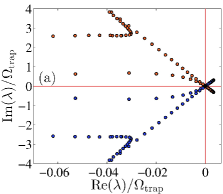
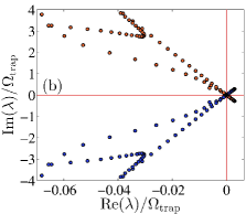
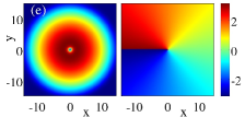
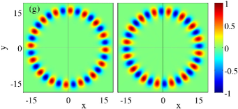
Fig. 7: (color online) Stability of steady states with different number of vortices for $\mu=5$, $\gamma=0.01$, $\Omega_{\rm trap}=0.2$, and $\Omega_{\rm rot}/\Omega=0.37$. (a)–(c) Stability spectra for configurations with 0, 1 and 2 vortices respectively. (d)–(f) Corresponding density (left subpanels) and phases (right subpanels) for these configurations. (g),(h) Most unstable eigenfunctions for configurations with 0 and 1 vortices, respectively. The left and right subpanels corresponds, respectively, to the real and imaginary parts of the most unstable eigenfunction.

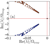
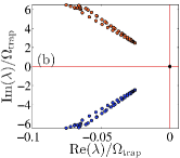
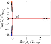
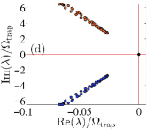
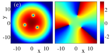
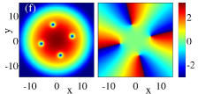
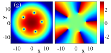
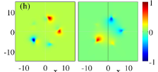
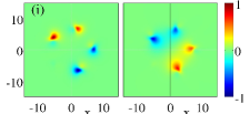
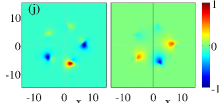
Fig. 8: (color online) Stability of steady states with different number of vortices for $\mu=5$, $\gamma=0.01$, $\Omega_{\rm trap}=0.2$, and $\Omega_{\rm rot}/\Omega_{\rm trap}=0.37$. (a)–(c) Stability spectra for configurations with 3, 4 and 5 vortices respectively. Note the unstable eigenvalues inside the circle for 5 vortices in panel (c). (d) Zoomed-in version of the stability spectrum for 5 vortices showing the eigenvalues corresponding to angular modes. (e)–(g) Density (left subpanels) and phases (right subpanels) for the configurations with 3, 4 and 5 vortices respectively. (h)–(j) Three most unstable eigenfunctions for the configuration with 5 vortices. The left and right subpanels corresponds, respectively, to the real and imaginary parts of the most unstable eigenfunction.

The final fate of the above selection mechanism can be, at least in part, be attributed to the fact that stationary corotating vortex polygons with different numbers of vortices have different stability properties for fixed parameter values. For instance, in Fig. 7 we depict the steady states, their stability spectra and their most unstable eigenmode for the case of $\mu=5$ for zero, one and two central vortices. As it is evident from the figure, the configurations bearing zero vortices and one vortex are unstable while the configuration with two vortices is stable. This corroborates the dynamical evolution depicted in Fig. 5 where the initial state with zero vortices destabilizes towards a transient state with one vortex that, in turn, destabilizes towards the final, stable steady state with two vortices. A similar stability analysis for $\mu=10$ (results not shown here) indicates that indeed the steady states with zero, one and two vortices are all unstable, while the state with three is perfectly stable; corroborating what is observed in the dynamical evolution depicted in Fig. 6.

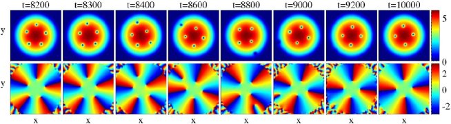
Fig. 9: (color online) Evolution of an unstable 5-vortex configuration. The initial state corresponds to the one in Fig. 8(g) (namely $\Omega_{\rm rot}/\Omega_{\rm trap}=0.37$, $\mu=5$, $\gamma=0.01$ and $\Omega_{\rm trap}=0.2$). The windows for density and phase are, respectively, $(x,y)\in[-17.5,17.5]\times[-17.5,17.5]$ and $(x,y)\in[-19,19]\times[-19,19]$. We invite the interested reader to see the full movie at this address: http:$\mathbin{/\mkern-4.0mu/}$nonlinear.sdsu.edu/ carreter/RotatingBEC.html [Movie#3].

The above results prompt the question of stability for configurations bearing an increasing number of vortices. For instance, as previously described, the configuration without vortices destabilizes when the rotation is increased, while configurations with one or more vortices become stable. However, polygonal configurations have a limit to the number of vortices that they can hold before becoming unstable (see Ref. [59] and references therein). This is depicted in Fig. 8 where the stability for polygonal vortex states with 3, 4 and 5 vortices for the case $\mu=5$ is examined. As it is clear from these results, the polygonal configurations with 3 and 4 vortices are indeed stable while the one with 5 vortices is unstable. Interestingly, the instability responsible for the breakup of the 5-vortex configuration is not an angular mode as in all the cases presented previously. In fact, it is clear that all the angular modes are stable as it can be seen from the zoomed-in version of the spectrum depicted in panel (d) of the figure where only the eigenvalues associated with angular modes are depicted. Nonetheless, the 5-vortex state is indeed unstable as is evident by the small cluster of unstable eigenvalues enclosed in the small circle in panel (c) of the figure. The eigenmodes associated with these unstable eigenvalues are depicted in panels (h)–(j). These symmetry breaking modes bring some of the vortices closer and others further apart from each other. It is precisely this mechanism that is responsible for the destabilization of the 5-vortex polygonal state as it is depicted in the snapshots of its evolution in Fig. 9. We invite the interested reader to see the full movie at this address: http:$\mathbin{/\mkern-4.0mu/}$nonlinear.sdsu.edu/ carreter/RotatingBEC.html [Movie#3]. Here, the initial steady state bearing a 5-vortex polygonal state destabilizes around $t=8200$, via a mode that pushes some vortices inward and other outward, eventually resulting in a stable 4-vortex polygonal state after one vortex is ejected towards the periphery of the cloud.

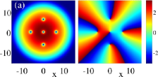
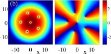
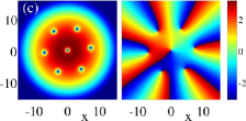
Fig. 10: (color online) Steady state configurations with $N$+1 vortices for $\Omega_{\rm rot}/\Omega_{\rm trap}=0.37$, $\mu=5$, $\gamma=0.01$, and $\Omega_{\rm trap}=0.2$. (a) 4+1 configuration, (b) 5+1 configuration, and (c) 6+1 configuration. All these configurations are stable for the chosen parameter values.

We have checked that the above phenomenology persists for other values of the dissipation coefficient $\gamma$. For instance, although the stability thresholds and the order ($m$) of the unstable modes for the vortex-less configuration are independent of $\gamma$, the growth rates for these instabilities are indeed dependent on dissipation (see also discussion below in Sec. 3.1). In particular, the larger $\gamma$ is, the larger the instability growth rates will be. Therefore, for larger values of $\gamma$ the instability will set in earlier and, more importantly, the pattern selection mechanism for the setlling of a cluster of vortices at the center of the cloud will be different. This is a direct consequence from the fact that the spiraling experienced by a vortex due to dissipation has a faster radial rate as $\gamma$ is increased [54]. A key effect of the slow down in the radial spiraling rate as $\gamma$ is decreased is that the pattern selection mechanism has “more time” to select votices and thus a smaller number of vortices is eventually pulled in from the periphery. This is precisely what we observe in numerical simulations where smaller values of $\gamma$ give rise to final configurations with a smaller number of vortices (results not shown here). For instance, for $\mu=5$ we find that for values of $\gamma$ of $0.5$, $0.2$, $0.1$, and $0.01,$ a vortex-less configuration evolves towards a stable steady state configuration with, respectively, 9, 7, 3, and 2 vortices. The same setup but for $\mu=10$ yields, respectively, 15, 11, 5, and 3 vortices. We invite the interested reader to see the full movies for all of these cases at this address: http:$\mathbin{/\mkern-4.0mu/}$nonlinear.sdsu.edu/ carreter/RotatingBEC.html [Movies#4–11].

Finally, let us briefly touch upon the existence of other relevant vortex configurations. The fact that polygonal configurations with large number of vortices lose stability prompts the important question: what are the remaining stable configurations of the system? For instance, in the absence of rotation, it has been shown that polygonal configurations become destabilized towards asymmetric configurations in a symmetry-breaking pitchfork bifurcation [60, 59] that has been observed in actual BEC experiments [25]. This instability occurs when the polygonal configuration increases its radius, namely, when the angular momentum of the vortex cluster is increased. In a similar manner, as we increase the rotation in the DGPE model (3) or as we increase the number of vortices, polygonal configurations lose stability. These instabilities can be manifested through angular modes (cf. the case of one vortex in Fig. 7) or through symmetry breaking modes (cf. the case for 5 vortices in Figs. 8 and 9). However, on the other hand, if ones starts with a polygonal state with an extra vortex at the center, the so-called $N$+1 vortex configurations, new stable states are produced [59] that might even be the ground states (i.e., the minimal energy states) of the system [60]. In Fig. 10 we depict three examples of these $N$+1 configurations for 4+1, 5+1, and 6+1 vortices. It is important to mention that these three configuration are indeed stable for the chosen parameter values. In fact, as the rotation increases and the number of vortices increases as well, more complex configurations relating to triangular (Abrikosov) vortex lattices arise.

Although our principal emphasis in this work lies in the identification of the most unstable mode that results in the instability of the state bearing no vortices in the context of Eq. (3), clearly numerous additional issues emerge from the above simulations. These concern the identification of the minimal energy state and the transition pathways resulting in different types of local or global attractors. We will briefly return to these questions in the context of future challenges in Section 4.

3 Overdamped NLS Model

3.1 Model and Numerical Results

Now a crucial observation allows us to explore the principal question raised above (about the dominant instability mode) in the context of slightly different and somewhat simpler model. The topological nature of the observed stability characteristics (i.e., of positive and negative energy modes) of the stationary state without vortices renders them robust and independent of the precise value of $\gamma$. In particular, for different values of $\gamma$, the actual size of the growth rates will change (in fact, the higher $\gamma$ is, the more unstable the relevant modes are). However, as can be also numerically checked, the ordering of the relevant eigenmodes will not be modified by the precise value of $\gamma$. That is to say, the same mode will become unstable at the same critical point (but with a different slope of Re$(\lambda)$ vs. $\Omega_{\rm rot}/\Omega_{\rm trap}$ in Fig. 3) for a different value of $\gamma$. Given this feature, we will hereafter choose to explore the “overdamped” limit of large $\gamma$, where in fact the Hamiltonian term in the left hand side of Eq. (3) is neglected in comparison to the $\gamma$-dependent dissipative one (and subsequently a time rescaling to absorb $\gamma$ is performed). Hence, we will work below with the “imaginary time” variant of the equation

$$u_{t}=\frac{1}{2}\Delta u-\frac{1}{2}\Omega_{\rm trap}^{2}x^{2}u+\mu u-|u|^{2}u-i\Omega_{\rm rot}u_{\theta},$$ (4)

which, based on the above arguments, should be sufficient to provide us with a prediction for the above instability when focusing on the vortex-less stationary state. In fact, this very statement will be double checked a posteriori in the next section.

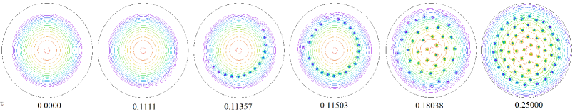
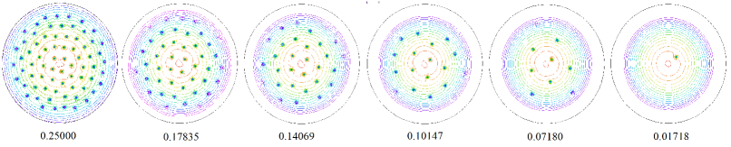
Fig. 11: (color online) Top: snapshots of the simulation of (4) with slowly varying $\Omega_{\rm rot}$ (as indicated) and with other parameters given by $\Omega_{\rm trap}=0.3538$ and $\mu=16.1$ (cf. Ref. [25]). Top row: $\Omega_{\rm rot}$ is slowly increased from 0 to 0.25 according to the formula (5). Middle row: $\Omega_{\rm rot}$ is slowly decreased from 0.25 to 0 according to the formula (6). Bottom row: number of vortices as a function of $\Omega_{\rm rot}$.

For motivational purposes, we start our presentation with two direct numerical experiments of Eq. (4).

Experiment 1: Slow Increase in Rotation. Let us allow for the rotation $\Omega_{\rm rot}$ to slowly increase from 0 to 0.25. More specifically, we start with $\Omega_{\rm rot}=0$, evolve the system until $t=2000$ (so that it effectively reaches its ground state under the imaginary time integration), then start increasing $\Omega_{\rm rot}$ linearly from 0 to 0.25 as $t$ varies from 2000 to 4000, and then finally we keep $\Omega_{\rm rot}=0.25$ until $t=10000$. In full, this experimental protocol can be summarized as:

$$\Omega_{\rm rot}\text{{\ = 0.25*min(max((t-2000)/2000,0),1)}}.$$ (5)

We used FlexPDE to simulate Eq. (4) with a uniform mesh with around 13000 triangles and adaptive time stepping.

Experiment 2: Slow Decrease in Rotation and Hysteresis. Let us now slowly decrease $\Omega_{\rm rot}$ from 0.25 to 0. In this complementary numerical experiment, we start with $\Omega_{\rm rot}=0.25$, and dynamically evolve the system until $t=2000$ to allow it to relax to its preferred vortex-lattice ground state profile. Then, we start decreasing $\Omega_{\rm rot}$ linearly to 0 as $t$ varies from 2000 to 4000, then keep $\Omega_{\rm rot}=0$ until $t=10000$. Mathematically again, this procedure can be summarized as:

$$\Omega_{\rm rot}\text{{\ = 0.25*(1-min(max((t-2000)/2000,0),1))}}.$$ (6)

Figure 11 presents a series of snapshots for each of the described experiments. There are a number of interesting observations to make here, as well as connections to provide with the discussion in the previous section. As $\Omega_{\rm rot}$ is ramped up, up to a critical rotational frequency no vortices arise. However, when they do arise (and despite the weak ramping), a considerable number of vortices seems to emerge asymmetrically (at first) yet nearly simultaneously. Gradually, as the rotation frequency increases, additional vorticity is “elicited” from the boundary, eventually leading the configuration to self-organize into a triangular vortex lattice as the final rotation frequency is reached. On the other hand, while the frequency is decreased towards $\Omega_{\rm rot}=0$, we can see that the process is clearly hysteretic, as for similar values of the rotation frequency as in the top panel, a considerably larger number of vortices appears to survive. This feature is most dramatic near the $\Omega_{\rm rot}=0$ (e.g. in the next to last panel of the bottom row) where numerous vortices appear to survive in this metastable dynamics, although clearly this is far from the ground state for that rotation frequency. Although there are numerous features that one may wish to explore on the basis of this dynamical simulation and the numerical results presented in the previous section, the one that we will focus on below (following up on the discussion of the earliest part of the previous section) concerns the instability dynamics of the dissipative variant of the GPE for the vortex-less steady state configuration. In particular, our expectation on the basis of the above direct simulation, as well as from the stability results presented is that a large $m$ mode is the one (predominantly) responsible for the destabilization of the vortex-less state, as is indeed observed in Fig. 11. We now proceed to analyze this trait mathematically in more detail at the level of Eq. (4).

3.2 Asymptotic Analysis

To start our analysis, we rescale Eq. (4) as follows:

$$x=\hat{x}\sqrt{\frac{\mu}{\frac{1}{2}\Omega_{\rm trap}^{2}}};\ \ u=\mu\hat{u};\ \ \ t=\frac{\hat{t}}{\mu}.\$$

After dropping the hats, we obtain

$$u_{t}=\varepsilon^{2}\Delta u+\left(1-\left|x\right|^{2}\right)u-\left|u\right|^{2}u-\Omega iu_{\theta},$$ (7)

where

$$\varepsilon=\frac{1}{2\mu}\sqrt{\Omega_{\rm trap}^{2}};\text{ \ \ }\Omega=\frac{\Omega_{\rm rot}}{\mu}.$$ (8)

This is equivalent to the following real system of PDEs for the real and imaginary parts of $u=v+iw$:

$$\left\{\begin{array}[]{c}v_{t}=\varepsilon^{2}\Delta v+\left(1-\left|x\right|^{2}\right)v-v^{3}-w^{2}v+\Omega w_{\theta},\\[4.30554pt] w_{t}=\varepsilon^{2}\Delta w+\left(1-\left|x\right|^{2}\right)w-w^{3}-v^{2}w-\Omega v_{\theta}.\end{array}\right.$$ (9)

Let $u=\eta_{0}$ be the radially-symmetric vortex-less state which satisfies:

$$0=\varepsilon^{2}\left(\eta_{0rr}+\frac{1}{r}\eta_{r}\right)+\left(1-r^{2}\right)\eta_{0}-\eta_{0}^{3}.$$ (10)

We linearize Eq. (9) around $\eta_{0}$, so that

$$v =\eta_{0}+e^{\lambda t}\phi(r),$$

$$w =0+e^{\lambda t}\psi(r),$$

to obtain the system

$$\left\{\begin{array}[]{c}\lambda\phi=\varepsilon^{2}\Delta\phi+\left(1-r^{2}-3\eta_{0}^{2}\right)\phi+\Omega\psi_{\theta},\\[8.61108pt] \lambda\psi=\varepsilon^{2}\Delta\psi+\left(1-r^{2}-\eta_{0}^{2}\right)\psi-\Omega\phi_{\theta}.\end{array}\right.$$ (11)

We now use the radial-polar decomposition for the perturbations of the form:

$$\phi(r,\theta)=e^{im\theta}\phi(r);\ \ \ \psi(r,\theta)=e^{im\theta}\psi\left(r\right),$$

to obtain

$$\left\{\begin{array}[]{c}\lambda\phi=\varepsilon^{2}\left(\phi_{rr}+\frac{1}{r}\phi_{r}-\frac{m^{2}}{r^{2}}\phi\right)+\left(1-r^{2}-3\eta_{0}^{2}\right)\phi+im\Omega\psi,\\[8.61108pt] \lambda\psi=\varepsilon^{2}\left(\psi_{rr}+\frac{1}{r}\psi_{r}-\frac{m^{2}}{r^{2}}\psi\right)+\left(1-r^{2}-\eta_{0}^{2}\right)\psi-im\Omega\phi,\end{array}\right.$$ (12)

Changing variables to $\psi=i\hat{\psi}$, and dropping the hat we then get a purely real system

$$\left\{\begin{array}[]{c}\lambda\phi=\varepsilon^{2}\left(\phi_{rr}+\frac{1}{r}\phi_{r}-\frac{m^{2}}{r^{2}}\phi\right)+\left(1-r^{2}-3\eta_{0}^{2}\right)\phi-m\Omega\psi,\\[8.61108pt] \lambda\psi=\varepsilon^{2}\left(\psi_{rr}+\frac{1}{r}\psi_{r}-\frac{m^{2}}{r^{2}}\psi\right)+\left(1-r^{2}-\eta_{0}^{2}\right)\psi-m\Omega\phi.\end{array}\right.$$ (13)

It is known that $\lambda<0$ when $\Omega=0$ and $\lambda>0$ for sufficiently large $\Omega$, as corroborated also by our numerical computations in the previous section. We therefore seek the instability threshold value for $\Omega$ for which $\lambda=0$. Thus, setting $\lambda=0$ in the eigenvalue problem, we obtain a modified eigenvalue problem for $m\Omega$ of the form:

$$\left\{\begin{array}[]{c}m\Omega\psi=\varepsilon^{2}\left(\phi_{rr}+\frac{1}{r}\phi_{r}-\frac{m^{2}}{r^{2}}\phi\right)+\left(1-r^{2}-3\eta_{0}^{2}\right)\phi,\\[8.61108pt] m\Omega\phi=\varepsilon^{2}\left(\psi_{rr}+\frac{1}{r}\psi_{r}-\frac{m^{2}}{r^{2}}\psi\right)+\left(1-r^{2}-\eta_{0}^{2}\right)\psi.\end{array}\right.$$ (14)

To obtain an intuitive understanding of the situation ahead of the detailed analysis, let us solve this problem numerically and then plot the graph of $m$ vs. $\Omega$. This is shown in Fig. 12(a) for $\varepsilon=0.04$ and $\varepsilon=0.02$. Recall that the large density/large chemical potential limit is associated with $\varepsilon\rightarrow 0$, hence the choice of suitably small $\varepsilon$. We find that this graph has a minimum which corresponds to the smallest value of $\Omega=\Omega_{c}$ for which the instability first manifests itself. Critically, for our discussion, this minimum depends on $\varepsilon$. Our goal is to characterize this minimum analytically, as well as to compute the corresponding wave number $m=m_{c}$ which should approximate the instability eigenmode that manifests itself as $\Omega$ increases and first crosses past $\Omega_{c}$.

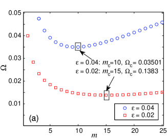
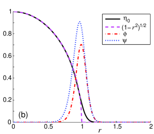
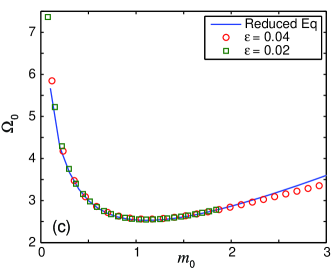
Fig. 12: (color online) (a) Solution to Eq. (14) showing $\Omega$ as a function of $m$. For a given mode $m$ on the horizontal axis, the vertical axis shows the threshold value of $\Omega$ for which this mode becomes unstable. The minimum of this graph is the overall threshold where the instability first sets in as $\Omega$ is increased from zero. (b) The profile of $\eta_{0}$, its Thomas-Fermi asymptotic approximation $\eta_{0}\sim\max((1-r^{2}),0)^{1/2}$, as well as the profile of the eigenfunctions corresponding to the problem (14). (c) Solution to the reduced system (16) as compared with the full system (14)

Figure 12(b) shows the plot of the leading eigenfunction for $\varepsilon=0.02$ with $m=15$ (corresponding to the critical threshold $\Omega_{c}=0.01383$). The relevant mode appears to be localized near $r\sim 1$. To capture this, we first have to resolve the corner layer of the steady state $\eta_{0}$ accurately near $r=1$. To that effect, we zoom in at $r=1$ and rescale according to:

$$r=1+\varepsilon^{2/3}y,\ \ \ \ \eta_{0}=\varepsilon^{1/3}U.$$

To leading order then we get from Eq. (10)

$$U_{yy}=2yU+U^{3},$$ (15)

which is a rescaled Painlevé II transcendent. It is well-known [61] that Eq. (15) admits a unique solution of the form

$$U\sim\left\{\begin{array}[]{c}C\,{\rm Ai}\left(\sqrt{2}y\right)\text{ as }y\rightarrow\infty\\[8.61108pt] \sqrt{-2y}\text{ \ \ as }y\rightarrow-\infty\end{array}\right.$$

where ${\rm Ai}$ is the Airy function and $C$ is a constant. Next, we use the same change of variables in the eigenvalue problem (14). We obtain then the reduced problem

$$\left\{\begin{array}[]{c}m_{0}\Omega_{0}\psi=\phi_{yy}-m_{0}^{2}\phi+\left(-2y-3U^{2}\right)\phi,\\[8.61108pt] m_{0}\Omega_{0}\phi=\psi_{yy}-m_{0}^{2}\psi+\left(-2y-U^{2}\right)\psi,\end{array}\right.$$ (16)

subject to the boundary conditions $\{\phi,\psi\}\rightarrow 0$ as $\left|y\right|\rightarrow\infty,$ where

$$m=\varepsilon^{-2/3}m_{0},\ \ \ \ \Omega=\varepsilon^{4/3}\Omega_{0}.$$ (17)

The problem (16) is solved numerically. The solution is shown in Fig. 12(c). Superimposed are the solutions to the full eigenvalue problem (14) for $\varepsilon=0.02$ and $\varepsilon=0.04$. It can thus be clearly observed that the scaling (17) is indeed correct. From Fig. 12, the minimum is attained at around $\Omega_{0,c}\approx 2.5$ (using the $\varepsilon=0.02$ curve). We now state this result (a numerically assisted proof for the result in provided in the appendix):

Main Result. There exist constants $\Omega_{0,c}$ and $m_{0,c}$ whose approximate values are

$$\Omega_{0,c}\approx 2.529,\ \ m_{0,c}\approx 1.111$$

such that the following is true. Let

$$\Omega_{c}=\varepsilon^{4/3}\Omega_{0,c},\ \ \ m_{c}=\varepsilon^{-2/3}m_{0,c}.$$

Then the vortex-less steady state (10) of Eq. (7) is stable when $\Omega<\Omega_{c}$ and becomes unstable as $\Omega$ crosses $\Omega_{c}$. The fastest-growing unstable mode corresponds to the oscillations of the boundary with the mode $m_{c}$.

Note that in terms of the original variables of Eq. (4), the critical threshold is given by

$$\Omega_{{\rm rot},c} =\Omega_{0,c}2^{-4/3}\mu^{-1/3}\Omega_{\rm trap}^{4/3}\approx 1.0036\mu^{-1/3}\Omega_{\rm trap}^{4/3};$$ (18)

$$m_{c} =m_{0,c}2^{2/3}\mu^{2/3}\Omega_{\rm trap}^{-2/3}\approx 1.76\mu^{2/3}\Omega_{\rm trap}^{-2/3}.$$ (19)

In Experiment 1 of the previous section depicted in Fig. 11, we had $\mu=16.1$ and $\Omega_{\rm trap}=0.3538$; these numbers correspond to the experimentally relevant setting of the work of Ref. [25]. This yields $\Omega_{{\rm rot},c}\approx 0.10$ and $m_{c}\approx 22.11$. This is in excellent agreement with the actual numerical simulations. In the top row of the figure, the instability becomes apparent around $\Omega_{\rm rot}\approx 0.11$. The instability actually sets in shortly prior to this, but it takes some time for it to fully mature. Once the instability is fully developed (fourth snapshot from the left), it results in 24 vortices, in fair agreement with the predicted value of $m_{c}\approx 22$ (it should be kept in mind that some of these vortices may be in the periphery of the cloud and hence may not be discernible in the density profile shown).

It is interesting finally to connect the results, e.g., with those of Figs. 1–3. In particular, as indicated in these results the left panel, e.g., of Fig. 1 corresponds to $\mu=5$, while the right one to $\mu=10$. According to the above scaling in the former case $\Omega_{{\rm rot},c}\approx 0.343$, while in the latter case $\Omega_{{\rm rot},c}\approx 0.272$. It can be seen that these critical points are in excellent agreement with the crossing points (from positive to negative energy modes) of the Hamiltonian system in Fig. 1, which involves the case of $\gamma=0$. They are also in excellent agreement with the stability thresholds of the dissipative system used in Figs. 2 and 3, although the latter only use $\gamma=0.01$. This comparison is given to also, a posteriori, justify the use of the analysis in the framework of the overdamped limit of Eq. (4) in the present context.

4 Conclusions and Future Challenges

In summary, in the present work, we have explored the instability in the presence of rotation of a dissipative variant of the GPE. We have connected this instability to the emergence of negative energy (or Krein signature) modes and the phenomenon of energetic (but not dynamical) instability of the radial vortex-less profile in the corresponding Hamiltonian system in the absence of dissipation. We have also connected it to the emergence of a real eigenvalue corresponding to suitably large $m$ (i.e., azimuthal order) for the dissipative system. Moreover, we have argued that this $m$ should be independent of $\gamma$, but should depend on the trapping frequency and on the chemical potential (i.e., the maximal atomic density) of the system. We have systematically developed a scaling law that provides the critical rotation frequency as a function of these parameters. We have confirmed the connection of this scaling with (a) the imaginary time (“overdamped”) model used; (b) the original Hamiltonian model and (c) the intermediate between the two dissipative Gross-Pitaevskii equation (DGPE) model. Using direct numerical simulations we have corroborated the prediction of our asymptotic analysis and observed that these unstable modes with high mode number $m$ indeed nucleate a large number of vortices at the periphery of the atomic cloud. However, we have found that despite the large number of vortices at the periphery, for the small values of $\gamma$ chiefly considered herein in the DGPE (yet somewhat larger than the ones that have been claimed as relevant for realistic experimental settings; see for a recent discussion [54]) few isolated vortices are pulled in sequentially towards the center of the cloud. The process whereby single vortices are singled out from the multi-vortex “necklace” at the periphery is a pattern selection mechanism based on symmetry-breaking. This sequential recruiting of peripheral vortices towards the cloud center saturates when reaching a highly symmetric configuration with a few vortices at the center of the cloud that is stable for the chosen parameters (chemical potential and rotation rate normalized by trap strength).

These results open a number of interesting directions for further exploration. Admittedly, our approach to the vortex nucleation problem is rather different from that of earlier works; see e.g. [62] and the relevant discussion of Ref. [8]. Nevertheless, it would be particularly interesting to explore in current experimental settings (such as e.g. [25]) whether a value of $\gamma$ can be “inferred” (e.g. from the spiraling motion of a vortex; see e.g. the relevant discussion of [54]). Based on such a value, our analysis and computation could provide diagnostics both for which eigenmode will cause the instability of the vortex-less state and for which asymptotic state may be experimentally observed.

Our observations also raise a related problem. Clearly, for different values of $\gamma$ ranging from the underdamped limit of Figs. 5–9 to the overdamped one of Fig. 11, (for same trap strength and chemical potential) we have conclusively argued that the same eigenmode and the same critical frequency are generically responsible for the observed instability. Yet, the instability manifestation has dramatically different outcomes for the different limits. This naturally prompts the question: what is the favored asymptotic state (depending on the value of $\gamma$) and how do we get there? The first and perhaps simpler question (that has been previously considered; see e.g. [63] for an early example) is presumably one of energetic comparisons of the states containing different numbers of vortices (incorporating their angular momentum contributions). The second and, arguably, more difficult question is one of transition state pathways that enable the nucleation of different multi-vortex configurations. The latter may be particularly worth exploring, especially since our results indicate that they will be dependent on features such as the thermal coupling parameter $\gamma$.

Appendix A A Numerically Assisted Proof Of The Main Result

Define the operators

$$\left\{\begin{array}[]{rl}L_{1}(\phi)\hskip-7.11317pt&:=\phi_{yy}+\left(-2y-3U^{2}\right)\phi,\\[8.61108pt] L_{2}(\phi)\hskip-7.11317pt&:=\phi_{yy}+\left(-2y-U^{2}\right)\phi.\end{array}\right.$$

As the first step, we show that both $L_{1}$ and $L_{2}$ are negative operators. First, note that that both are self-adjoint so it suffices to show that all eigenvalues are real non-positive. To show that $L_{2}$ is negative, simply note that $L_{2}(U)=0$. Since $U$ is positive, Sturm’s eigenvalue oscillation theorem then implies that $\lambda=0$ is the largest eigenvalue of $L_{2}$, hence $L_{2}$ is negative. The negativity of $L_{1}$ follows from the fact that $2y+3U^{2}>0$ for all $y$; see Ref. [64].

The problem (16) may then be reformulated as

$$m_{0}\Omega_{0}=\pm\sqrt{\mu};\ \ \ \mu\phi=(L_{1}-m_{0}^{2})\cdot(L_{2}-m_{0}^{2})\,\phi.$$ (20)

It follows by the negativity of $L_{1}-m_{0}^{2}$ and $L_{2}-m_{0}^{2}$ that $\mu$ is real and positive so that the curve $\Omega_{0}=\Omega_{0}(m_{0})$ is well defined.

Finally, we show that the curve $\Omega_{0}=\Omega_{0}(m_{0})$ has a minimum for some strictly positive value of $m_{0}$. For large $m_{0}$ we find that $\mu\sim m_{0}^{4}$ and hence $\Omega_{0}\sim m_{0}$. On the other hand, numerical computations of (20) with $m_{0}=0$ yield $\mu=0.1576654>0$. It follows that $\Omega_{0}\sim 0.39707/m_{0}$ as $m_{0}\rightarrow 0^{+}$. Thus $\Omega_{0}$ blows up at the endpoints $m_{0}\rightarrow 0^{+}$ and $m_{0}\rightarrow\infty$, which shows that this curve indeed has a minimum.

Acknowledgments. We are grateful to Dmitry Pelinovsky for useful discussions and for insights leading to the proof of the Main Result (Appendix A). R.C.G. acknowledges support from DMS-1309035. P.G.K. acknowledges support from the National Science Foundation under grants DMS-1312856, from ERC and FP7-People under grant IRSES-605096, from the US-AFOSR under grant FA9550-12-10332, and from the Binational (US-Israel) Science Foundation through grant 2010239. P.G.K.’s work at Los Alamos is supported in part by the U.S. Department of Energy. T.K. was supported by NSERC Discovery Grant No. RGPIN-33798 and Accelerator Supplement Grant No. RGPAS/461907.

References

- [1] L.M. Pismen, Vortices in Nonlinear Fields (Clarendon, UK, 1999).
- [2] Yu.S. Kivshar and B. Luther-Davies, Physics Reports 298, 81–197 (1998).
- [3] Y.S. Kivshar, J. Christou, V. Tikhonenko, B. Luther-Davies and L. Pismen, Optics Comm. 152, 198–206 (1998).
- [4] H.J. Lugt, Vortex Flow in Nature and Technology (John Wiley and Sons, Inc., New York, 1983).
- [5] D.L. Whitaker and J. Edwards, Science 329, 406 (2010).
- [6] F. Dalfovo, S. Giorgini, L.P. Pitaevskii and S. Stringari, Rev. Mod. Phys. 71, 463–512 (1999).
- [7] C.J. Pethick and H. Smith, Bose-Einstein condensation in dilute gases, (Cambridge University Press, Cambridge, 2002).
- [8] L.P. Pitaevskii and S. Stringari, Bose-Einstein Condensation, Oxford University Press (Oxford, 2003).
- [9] M.R. Matthews, B.P. Anderson, P.C. Haljan, D.S. Hall, C.E. Wieman, and E.A. Cornell, Phys. Rev. Lett. 83, 2498–2501 (1999).
- [10] J.E. Williams and M.J. Holland, Nature 401, 568–572 (1999).
- [11] K.W. Madison, F. Chevy, W. Wohlleben, and J. Dalibard, Phys. Rev. Lett. 84, 806 (2000).
- [12] A. Recati, F. Zambelli, and S. Stringari, Phys. Rev. Lett. 86, 377 (2001).
- [13] S. Sinha and Y. Castin, Phys. Rev. Lett. 87, 190402 (2001).
- [14] K.W. Madison, F. Chevy, V. Bretin, and J. Dalibard, Phys. Rev. Lett. 86, 4443 (2001).
- [15] C. Raman, J.R. Abo-Shaeer, J.M. Vogels, K. Xu, and W. Ketterle, Phys. Rev. Lett. 87, 210402 (2001).
- [16] J.R. Abo-Shaeer, C. Raman, J.M. Vogels, and W. Ketterle, Observation of vortex lattices in Bose-Einstein condensates, Science 292, 476–479 (2001).
- [17] R. Onofrio, C. Raman, J.M. Vogels, J.R. Abo-Shaeer, A.P. Chikkatur, and W. Ketterle, Phys. Rev. Lett. 85, 2228 (2000).
- [18] D.R. Scherer, C.N. Weiler, T.W. Neely, and B.P. Anderson, Phys. Rev. Lett. 98, 110402 (2007).
- [19] A.E. Leanhardt, A. Görlitz, A.P. Chikkatur, D. Kielpinski, Y. Shin, D.E. Pritchard, and W. Ketterle, Phys. Rev. Lett. 89, 190403 (2002); Y. Shin, M. Saba, M. Vengalattore, T.A. Pasquini, C. Sanner, A.E. Leanhardt, M. Prentiss, D.E. Pritchard, and W. Ketterle, Phys. Rev. Lett. 93, 160406 (2004).
- [20] C.N. Weiler, T.W. Neely, D.R. Scherer, A.S. Bradley, M.J. Davis, B.P. Anderson, Nature 455, 948–951 (2008).
- [21] D.V. Freilich, D.M. Bianchi, A.M. Kaufman, T.K. Langin, and D.S. Hall, Science 329, 1182–1185 (2010).
- [22] T.W. Neely, E.C. Samson, A.S. Bradley, M.J. Davis, B.P. Anderson, Phys. Rev. Lett. 104, 160401 (2010).
- [23] S. Middelkamp, P.J. Torres, P.G. Kevrekidis, D.J. Frantzeskakis, R. Carretero-González, P. Schmelcher, D.V. Freilich, and D.S. Hall, Phys. Rev. A 84, 011605(R) (2011).
- [24] J.A. Seman, E.A.L. Henn, M. Haque, R.F. Shiozaki, E.R.F. Ramos, M. Caracanhas, P. Castilho, C. Castelo Branco, P.E.S. Tavares, F.J. Poveda-Cuevas, G. Roati, K.M.F. Magalhaes, and V.S. Bagnato, Phys. Rev. A 82, 033616 (2010).
- [25] R. Navarro, R. Carretero-González, P.J. Torres, P.G. Kevrekidis, D.J. Frantzeskakis, M.W. Ray, E. Altuntaş, and D.S. Hall, Phys. Rev. Lett. 110, 225301 (2013).
- [26] N.P. Proukakis, S.A. Gardiner, M.J. Davis, and M.H. Szymanska (Eds.), Quantum Gases: Finite Temperature and Non-Equilibrium Dynamics (Imperial College Press, London, 2013).
- [27] S. Burger, K. Bongs, S. Dettmer, W. Ertmer, K. Sengstock, A. Sanpera, G.V. Shlyapnikov, and M. Lewenstein, Phys. Rev. Lett. 83, 5198 (1999).
- [28] K. Bongs, S. Burger, S. Dettmer, D. Hellweg, J. Arlt, W. Ertmer, and K. Sengstock, C. R. Acad. Sci. Paris 2, 671 (2001).
- [29] J. Denschlag, J.E. Simsarian, D.L. Feder, C.W. Clark, L.A. Collins, J. Cubizolles, L. Deng, E.W. Hagley, K. Helmerson, W.P. Reinhardt, S.L. Rolston, B.I. Schneider, and W.D. Phillips, Science 287, 97 (2000).
- [30] T. Yefsah, A.T. Sommer, M.J.H. Ku, L.W. Cheuk, W.J. Ji, W.S. Bakr, and M.W. Zwierlein, Nature 499, 426 (2013)
- [31] P.O. Fedichev, A.E. Muryshev, and G.V. Shlyapnikov, Phys. Rev. A 60, 3220 (1999).
- [32] A. Muryshev, G.V. Shlyapnikov, W. Ertmer, K. Sengstock, and M. Lewenstein, Phys. Rev. Lett. 89, 110401 (2002).
- [33] S.P. Cockburn, H.E. Nistazakis, T.P. Horikis, P.G. Kevrekidis, N.P. Proukakis, and D.J. Frantzeskakis, Phys. Rev. Lett. 104, 174101 (2010); ibid. Phys. Rev. A 84, 043640 (2011).
- [34] N.P. Proukakis, N.G. Parker, C.F. Barenghi, and C.S. Adams, Phys. Rev. Lett. 93, 130408 (2004).
- [35] B. Jackson, N.P. Proukakis, and C.F. Barenghi, Phys. Rev. A 75, 051601 (2007); B. Jackson, C.F. Barenghi, and N.P. Proukakis, J. Low Temp. Phys. 148, 387 (2007);
- [36] W.H. Zurek, Phys. Rev. Lett. 102, 105702 (2009); B. Damski, and W.H. Zurek, Phys. Rev. Lett. 104, 160404 (2010).
- [37] A.D. Martin and J. Ruostekoski, Phys. Rev. Lett. 104 (2010) 194102 (2010); A.D. Martin and J. Ruostekoski, New J. Phys. 12, 055018 (2010).
- [38] D.M. Gangardt and A. Kamenev, Phys. Rev. Lett. 104, 190402 (2010).
- [39] K.J. Wright and A.S. Bradley, arXiv:1104.2691.
- [40] L.P. Pitaevskii, Zh. Eksp. Teor. Fiz. 35, 408 (1958) [Sov. Phys. JETP 35, 282 (1959)].
- [41] A.A. Penckwitt, R.J. Ballagh, and C.W. Gardiner, Phys. Rev. Lett. 89, 260402 (2002).
- [42] B. Jackson and N.P. Proukakis, J. Phys. B: At. Mol. Opt. Phys. 41, 203002 (2008).
- [43] P.B. Blakie, A.S. Bradley, M.J. Davis, R.J. Ballagh, and C.W. Gardiner, Adv. Phys. 57, 363 (2008).
- [44] A. Griffin, T. Nikuni, and E. Zaremba, Bose-Condensed Gases at Finite Temperatures (Cambridge University Press, Cambridge, 2009).
- [45] H.T.C. Stoof, J. Low Temp. Phys. 114, 11 (1999); H.T.C. Stoof, and M.J. Bijlsma, J. Low Temp. Phys. 124, 431 (2001).
- [46] S.P. Cockburn and N.P. Proukakis, Laser Phys. 19, 558 (2009).
- [47] B. Jackson, N.P. Proukakis, C.F. Barenghi, and E. Zaremba, Phys. Rev. A 79, 053615 (2009).
- [48] A.J. Allen, E. Zaremba, C.F. Barenghi, N.P. Proukakis, Phys. Rev. A 87, 013630 (2013).
- [49] S. Middelkamp, P.G. Kevrekidis, D.J. Frantzeskakis, R. Carretero-González, P. Schmelcher J. Phys. B 43, 155303 (2010).
- [50] S.J. Rooney, A.S. Bradley, and P.B. Blakie, Phys. Rev. A 81, 023630 (2010).
- [51] T.M. Wright, A.S. Bradley, and R.J. Ballagh, Phys. Rev. A 80, 053624 (2009)
- [52] R.A. Duine, B.W.A. Leurs, and H.T.C. Stoof, Phys. Rev. A 69, 053623 (2004).
- [53] A.S. Bradley, C.W. Gardiner, arXiv:cond-mat/0509592.
- [54] D. Yan, R. Carretero-González, D.J. Frantzeskakis, P.G. Kevrekidis, N.P. Proukakis, and D. Spirn, Phys. Rev. A 89, 043613 (2014).
- [55] P.G. Kevrekidis, D.J. Frantzeskakis, and R. Carretero-González, Emergent Nonlinear Phenomena in Bose-Einstein Condensates, Springer-Verlag (Berlin, 2008).
- [56] See for a detailed discussion of such modes: D.V. Skryabin, Phys. Rev. A 63, 013602 (2000).
- [57] T. Kapitula, P.G. Kevrekidis and B. Sandstede, Physica D 195, 263 (2004).
- [58] B. Wu and Q. Niu, New J. Phys. 5, 104 (2003).
- [59] T. Kolokolnikov, P.G. Kevrekidis, and R. Carretero-González, Proc. R. Soc. A 470, 2014004. (2014).
- [60] A.V. Zampetaki, R. Carretero-González, P.G. Kevrekidis, F.K. Diakonos, and D.J. Frantzeskakis, Phys. Rev. E 88, 042914 (2014).
- [61] M.J. Ablowitz, and P.A. Clarkson, Solitons, Nonlinear Evolution Equations and Inverse Scattering, Cambridge University Press (Cambridge, 1991).
- [62] E. Lundh, C.J. Pethick, and H. Smith, Phys. Rev. A 55, 2126–2131 (1997).
- [63] Y. Castin, R. Dum, Eur. Phys. J. D 7, 399–412 (1999).
- [64] See Lemma 2.2 on p. 60 in C. Gallo and D. Pelinovsky, Asymptotic Analysis 73, 53 (2011).