A directed search for gravitational waves from Scorpius X-1 with initial LIGO

Abstract

We present results of a search for continuously-emitted gravitational radiation, directed at the brightest low-mass X-ray binary, Scorpius X-1. Our semi-coherent analysis covers 10 days of LIGO S5 data ranging from 50–550 Hz, and performs an incoherent sum of coherent $\mathcal{F}$-statistic power distributed amongst frequency-modulated orbital sidebands. All candidates not removed at the veto stage were found to be consistent with noise at a $1\%$ false alarm rate. We present Bayesian 95% confidence upper limits on gravitational-wave strain amplitude using two different prior distributions: a standard one, with no a priori assumptions about the orientation of Scorpius X-1; and an angle-restricted one, using a prior derived from electromagnetic observations. Median strain upper limits of $1.3\times 10^{-24}$ and $8\times 10^{-25}$ are reported at 150 Hz for the standard and angle-restricted searches respectively. This proof of principle analysis was limited to a short observation time by unknown effects of accretion on the intrinsic spin frequency of the neutron star, but improves upon previous upper limits by factors of ${\sim}1.4$ for the standard, and 2.3 for the angle-restricted search at the sensitive region of the detector.

I Introduction

Recycled neutron stars are a likely source of persistent, quasi-monochromatic gravitational waves detectable by ground-based interferometric detectors. Emission mechanisms include thermocompositional and magnetic mountains Bonazzola and Gourgoulhon (1996); Ushomirsky et al. (2000); Melatos and Payne (2005); Vigelius and Melatos (2009); Priymak et al. (2011); Haskell et al. (2006), unstable oscillation modes Owen et al. (1998) and free precession Jones (2002). If the angular momentum lost to gravitational radiation is balanced by the spin-up torque from accretion, the gravitational wave strain $h_{\text{\tiny{\emph{0}}}}$ can be estimated independently of the microphysical origin of the quadrupole and is proportional to the observable X-ray flux $F_{x}$ and spin frequency $\nu_{\text{s}}$  Wagoner (1984); Bildsten (1998) via $h_{\text{\tiny{\emph{0}}}}\propto\left({F_{\text{\tiny{X}}}}/{\nu_{\text{s}}}\right)^{1/2}$. Given the assumption of torque balance, the strongest gravitational wave sources are those that are most proximate with the highest accretion rate and hence X-ray flux, such as low-mass X-ray binary (LMXB) systems. In this sense the most luminous gravitational wave LMXB source is Scorpius X-1 (Sco X-1).

The plausibility of the torque-balance scenario is strengthened by observations of the spin frequencies $\nu_{\text{s}}$ of pulsating or bursting LMXBs, which show them clustered in a relatively narrow band from $270\leqslant\nu_{\text{s}}\leqslant 620$ Hz Chakrabarty et al. (2003), even though their ages and accretions rates imply that they should have accreted enough matter to reach the centrifugal break-up limit $\nu_{\text{max}}{\sim}1400$ Hz Cook et al. (1994) of the neutron star. The gravitational wave spin-down torque scales as $\nu_{\text{s}}^{5}$, mapping a wide range of accretion rates into a narrow range of equilibrium spins, so far conforming with observations. Alternative explanations for the clustering of LMXB spin periods involving disc accretion physics have been proposed Haskell et al. (2014). Although this explanation suggests that gravitational radiation is not required to brake the spin-up of the neutron star, it does not rule out gravitational emission from these systems. The gravitational-wave torque-balance argument is used here as an approximate bound.

The initial instruments installed in the Laser Interferometer Gravitational Wave Observatory (LIGO) consisted of three Michelson interferometers, one with 4-km orthogonal arms at Livingston, LA, and two collocated at Hanford, CA, with 4 km and 2 km arms. Initial LIGO achieved its design sensitivity during its fifth science run (between November 2005 and October 2007 ) Abbott et al. (2009); Abadie et al. (2010) and is currently being upgraded to the next-generation Advanced LIGO configuration, which is expected to improve its sensitivity ten-fold in strain Harry and the LIGO Scientific Collaboration (2010).

Three types of searches have previously been conducted with LIGO data for Sco X-1. The first, a coherent analysis using data from LIGO’s second science run (S2), was computationally limited to six-hour data segments. It placed a wave-strain upper limit at $95\%$ confidence of $h_{0}^{95}\approx 2\times 10^{-22}$ for two 20 Hz bands between 464 – 484 Hz and 604 – 626 Hz Abbott et al. (2007). The second, employing a radiometer technique Ballmer (2006), was conducted using all 20 days of LIGO S4 data Abbott et al. (2007). It improved the upper limits on the previous (S2) search by an order of magnitude in the relevant frequency bands but did not yield a detection. The same method was later applied to S5 data and reported roughly a five-fold sensitivity improvement over the S4 results Abadie et al. (2011). The S5 analysis returned a median $90\%$ confidence root-mean-square strain upper limit of $h^{90}_{\text{rms}}=7\times 10^{-25}$ at 150 Hz, the most sensitive detector frequency (this converts to $h_{0}^{95}\approx 2\times 10^{-24}$ str ; rad ; Messenger (2010)). Thirdly, an all-sky search for continuous gravitational waves from sources in binary systems, which looks for patterns caused by binary orbital motion doubly Fourier-transformed data (TwoSpect), was adapted to search the Sco X-1 sky position, and returned results in the low frequency band from $20-57.25$ Hz  Aasi et al. (2014).

Here we implement a new search for gravitational waves from sources in known binary systems, with unknown spin frequency, initially directed at Sco X-1 on LIGO S5 data to demonstrate feasibility. Values of the coherent, matched-filtered $\mathcal{F}$-statistic Jaranowski et al. (1998) are incoherently summed at the locations of frequency-modulated sidebands. This multi-stage, semi-coherent, analysis yields a new detection statistic, denoted the $\mathcal{C}$-statistic Messenger and Woan (2007); Sammut et al. (2014). A similar technique was first employed in electromagnetic searches for radio pulsars Ransom et al. (2003). We utilise this technique to efficiently deal with the large parameter space introduced by the orbital motion of a source in a binary system.

A brief description of the search is given in Sec. II, while the astrophysical target source and its associated parameter space are discussed in Sec. III. Section IV outlines the search method, reviews the pipeline, discusses the selection and preprocessing of LIGO S5 data, and explains the post-processing procedure. Results of the search, including upper limits of gravitational wave strain, are presented and discussed in Sections V and VI, respectively and restated in Sec. VII.

II Search Method

For a gravitational wave source in a binary system, the frequency of the signal is Doppler modulated by the orbital motion of the source with respect to the Earth  Ransom et al. (2003); Messenger and Woan (2007); Sammut et al. (2014). The semi-coherent sideband search method involves the incoherent summation of frequency modulated sidebands of the coherent $\mathcal{F}$-statistic  Jaranowski et al. (1998); Messenger and Woan (2007); Sammut et al. (2014).

The first step in the sideband search is to calculate the coherent $\mathcal{F}$-statistic as a function of frequency, assuming only a fixed sky position. Knowing the sky position, one can account for the phase evolution due to the motion of the detector. For sources in binary systems, the orbital motion splits the signal contribution to the $\mathcal{F}$-statistic into approximately $M=2m+1$ sidebands separated by $1/P$ in frequency, where $m=\text{ceiling}(2\pi f_{\text{\tiny{\emph{0}}}}a_{\text{\tiny{\emph{0}}}})$ , $f_{\text{\tiny{\emph{0}}}}$ is the intrinsic gravitational wave frequency, $a_{\text{\tiny{\emph{0}}}}$ is the light travel time across the semi-major axis of the orbit, and $P$ is the orbital period. Knowledge of $P$ and $a_{\text{\tiny{\emph{0}}}}$, allows us to construct an $\mathcal{F}$-statistic sideband template.

The second stage of the sideband pipeline is the calculation of the $\mathcal{C}$-statistic, where we convolve the sideband template with the coherent $\mathcal{F}$-statistic. The result is an incoherent sum of the signal power at each of the potential sidebands as a function of intrinsic gravitational wave frequency. For our template we use a flat comb function with equal amplitude teeth (see Fig. 1 of Sammut et al. (2014)), and hence, for a discrete frequency bin $f_{k}$, the template is given by

$$\mathcal{T}(f_{k})=\sum_{j=-m^{\prime}}^{m^{\prime}}\delta_{k\,l_{[j]}},$$ (1)

where $m^{\prime}=\text{ceiling}(2\pi f^{\prime}a^{\prime})$ depends on search frequency $f^{\prime}$ and the semi-major axis $a^{\prime}$ used to construct the template (see Sec. III.4) . The index $l_{[j]}$ of the Kronecker delta-function is defined as

$$l_{[j]}\equiv\texttt{round}\left(\frac{j}{P^{\prime}\Delta_{f}}\right),$$ (2)

for a frequency bin width $\Delta f$, where round() returns the closest integer, and $P^{\prime}$ denotes our best guess at the orbital period. The following convolution then yields the $\mathcal{C}$-statistic,

$$\mathcal{C}(f_{k}) = \left(2\mathcal{F}\ast\mathcal{T}\right)(f_{k})$$ (3)

$$= \sum_{j=-m^{\prime}}^{m^{\prime}}2\mathcal{F}(f_{k-l_{[j]}}),$$ (4)

where the form of $2\mathcal{F}$ is described in Jaranowski et al. (1998); Prix (2007); Sammut et al. (2014). We therefore obtain this final statistic as a function of frequency evaluated at the same discrete frequency bins $f_{k}$ on which the input $\mathcal{F}$-statistic is computed.

III Parameter space

Sco X-1 is the brightest LMXB, and the first to be discovered in 1962 Giacconi et al. (1962), located 2.8 kpc away Bradshaw et al. (1999), in the constellation Scorpius. Source parameters inferred from a variety of electromagnetic measurements are displayed in Table 1. Assuming that the gravitational radiation and accretion torques balance, we obtain an indirect upper limit on the gravitational wave strain amplitude for Sco X-1 as a function of $\nu_{\text{s}}$ . Assuming fiducial values for the mass $M=1.4M_{\odot}$, radius $R=10$ km Steeghs and Casares (2002), and moment of inertia $I=10^{38}$ kg m² Bradshaw et al. (1999) gives

$$h_{\text{\tiny{\emph{0}}}}^{\text{EQ}}\approx 3.5\times 10^{-26}\left(\frac{300\textrm{Hz}}{\nu_{\text{s}}}\right)^{1/2}.$$ (5)

Equation 5 assumes that all the angular momentum due to accretion is transferred to the star and converted into gravitational waves, providing an upper limit on the gravitational wave strain  .

Table 1: Sco X-1 observed parameters

Parameter (Name and Symbol)				Value [Reference]
X-ray flux		$F_{\text{\tiny{X}}}$		$4\times 10^{-7}$ erg cm-2 s-1	Watts et al. (2008)
Distance		$D$		$2.8\pm 0.3$ kpc	Bradshaw et al. (1999)
Right ascension		$\alpha$		16h 19m 55.0850s	Bradshaw et al. (1999)
Declination		$\delta$		${-15}^{\circ}$ 38’ 24.9”	Bradshaw et al. (1999)
Sky Position angular resolution		$\Delta\beta$		0.3 mas	Bradshaw et al. (1999)
Proper motion		$\mu$		14.1 mas yr-1	Bradshaw et al. (1999)
Orbital period		$P$		$68023.70496\pm 0.0432$ s	Galloway et al. (2014)
Projected semi-major axis		$a_{\text{\tiny{\emph{0}}}}$		1.44 $\pm 0.18$ s	Steeghs and Casares (2002)
Polarization angle		$\psi$		$234\pm 3^{\circ}$	Fomalont et al. (2001)
Inclination angle		$\iota$		$44\pm 6^{\circ}$	Fomalont et al. (2001)

Optical observations of Sco X-1 have accurately determined its sky position and orbital period and, less accurately, the semi-major axis Gottlieb et al. (1975); Bradshaw et al. (1999); Steeghs and Casares (2002); Galloway et al. (2014). The rotation period remains unknown, since no X-ray pulsations or bursts have been detected. Although twin kHz quasi-periodic oscillations have been observed in the contiuous X-ray flux with separations in the range $240-310$ Hz, there is no consistent and validated method that supports a relationship between the QPO frequencys and the spin frequency of the neutron star (see Watts (2012) for a review). We therefore assume the spin period is unknown and search over a range of $\nu_{\text{s}}$. We also assume a circular orbit, which is expected by the time mass transfer occurs in LMXB systems. In general, orbital eccentricity causes a redistribution of signal power amongst the existing circular orbit sidebands and will cause negligible leakage of signal power into additional sidebands at the boundaries of the sideband structure. Orbital eccentricity also has the effect of modifying the phase of each sideband. However, the standard sideband search is insensitive to the phase of individual sidebands.

This section defines the parameter space of the sideband search, quantifying the accuracy with which each parameter is and/or needs to be known. The parameters and their uncertainties are summarised in Table 2.

Table 2: Derived Sideband search parameters

Parameter	Symbol	Value
Spin limited observation time	$T_{\text{s}}^{\text{spin}}$	13 days
Period limited observation time	$T_{\text{s}}^{\text{Porb}}$	50 days
Maximum sky position error	$\Delta\beta^{\text{max}}$	300 mas
Maximum proper motion	$\mu_{\beta}^{\text{max}}$	3000 mas yr-1
Neutron star inclination	$\iota_{\text{\tiny{EM}}}$	$44^{\circ}\pm 6^{\circ}$
- EM independent	$\cos\iota$	$[-1,\;1]$
Gravitational wave polaristion	$\psi_{\text{\tiny{EM}}}$	$234^{\circ}\pm 4^{\circ}$
- EM independent	$\psi$	$[-\tfrac{\pi}{4},\;\tfrac{\pi}{4}]$

III.1 Spin frequency

The (unknown) neutron star spin period is likely to fluctuate due to variations in the accretion rate $\dot{M}$. The coherent observation time span $T_{\text{s}}$ determines the size of the frequency bins in the calculation of the $\mathcal{F}$-statistic, along with an over-resolution factor $r$ defined such that a frequency bin is $1/(rT_{\text{s}})$ Hz wide. To avoid sensitivity loss due to the signal wandering outside an individual frequency bin, we restrict the coherent observation time to less than the spin limited observation time $T_{\text{s}}^{\text{spin}}$ so that the signal is approximately monochromatic. Conservatively, assuming the deviation of the accretion torque from the mean flips sign randomly on the timescale $t_{s}{\sim}$ days Ushomirsky et al. (2000), $\nu_{\text{s}}$ experiences a random walk which would stay within a Fourier frequency bin width for observation times less than $T_{\text{s}}^{\text{spin}}$ given by

$$T_{\text{s}}^{\text{spin}}=\left(\frac{2\pi I}{rN_{a}}\right)^{2/3}\left(\frac{1}{t_{s}}\right)^{1/3},$$ (6)

where $I=\tfrac{2}{5}MR^{2}$ is the moment of inertia of a neutron star with mass $M$ and radius $R$, $N_{a}=\dot{M}(GMR)^{1/2}$ is the mean accretion torque and $G$ is the gravitational constant.

For Sco X-1, with fiducial values for $M$, $R$, and $I$ as described earlier, and assuming $t_{s}=1$ day (comparable to the timescale of fluctuations in X-ray flux Bildsten et al. (1997)), $T_{\text{s}}^{\text{spin}}=13$ days. We choose observation time span $T_{\text{s}}=10$ days to fit safely within this restriction.

III.2 Orbital period

The orbital period $P_{\text{orb}}$ sets the frequency spacing of the sidebands. Uncertainties in this parameter will therefore translate to offsets in the spacing between the template and signal sidebands. The maximum coherent observation timespan $T_{\text{s}}^{\text{Porb}}$ allowed for use with a single template value of $P_{\text{orb}}$ is determined by the uncertainty $\Delta P_{\text{orb}}$ and can be expressed via

$$T_{\text{s}}^{\text{Porb}}\approx\frac{{P_{\text{orb}}}^{2}}{2\pi rf_{\text{\tiny{\emph{0}}}}a_{\text{\tiny{\emph{0}}}}|\Delta P|},$$ (7)

where a frequency bin in the $\mathcal{F}$-statistic has width $1/rT_{\text{s}}$ as explained above, and $f_{\text{\tiny{\emph{0}}}}$ and $a_{\text{\tiny{\emph{0}}}}$ are the intrinsic gravitational wave frequency and light crossing time of the projected semi-major axis respectively. For a Sco X-1 search with $r=2$ at $f_{\text{\tiny{\emph{0}}}}=1$ kHz, one finds $T_{\text{s}}^{\text{Porb}}=50$ days, longer than the maximum duration allowed by spin wandering (i.e. $T_{\text{s}}^{\text{Porb}}>T_{\text{s}}^{\text{spin}}$). Choosing $f_{\text{\tiny{\emph{0}}}}=1$ kHz gives a conservative limit for $T_{\text{s}}^{\text{Porb}}$ since lower frequencies will give higher values, and we only search up to 550 Hz. Thus we can safely assume the orbital period is known exactly for a search spanning $T_{\text{s}}\leqslant$ 50 days.

III.3 Sky position and proper motion

Knowledge of the source sky position is required to demodulate the effects of detector motion with respect to the barycentre of the source binary system (due to the Earth’s diurnal and orbital motion) when calculating the $\mathcal{F}$-statistic. We define an approximate worst-case error in sky position $\Delta\beta^{\text{max}}$ as that which would cause a maximum gravitational wave phase offset of 1 rad, giving us

$$|\Delta\beta^{\text{max}}|=\left(2\pi f_{\text{\tiny{\emph{0}}}}R_{\text{o}}\right)^{-1},$$ (8)

where $R_{\text{o}}$ is the Earth-Sun distance (1 AU). Additionally, the proper motion of the source also needs to be taken into account. If the motion is large enough over the observation time it will contribute to the phase error in the same way as the sky position error. The worst case proper motion $\mu_{{}_{\beta}}^{\text{max}}$ can therefore be determined similarly, viz.

$$|\mu_{{}_{\beta}}^{\text{max}}|\leqslant(2\pi f_{\text{\tiny{\emph{0}}}}R_{\text{o}}T_{\text{s}})^{-1}$$ (9)

For a 10-day observation at $f_{\text{\tiny{\emph{0}}}}=1$ kHz, one finds $\Delta\beta=100$ mas and $\mu_{{}_{\beta}}^{\text{max}}=3000\text{ mas yr}^{-1}$.

The sky position of Sco X-1 has been measured to within 0.3 mas, with a proper motion of 14.1 mas yr^-1 Bradshaw et al. (1999). These are well within the allowed constraints, validating the approximation that the sky position can be assumed known and fixed within our analysis.

III.4 Semi-major axis

The semi-major axis determines the number of sidebands in the search template. Its uncertainty affects the sensitivity of the search independently of the observation time. To avoid the template width being underestimated, we construct a template using a semi-major axis $a^{\prime}$ given by the (best guess) observed value $a$ and its uncertainty $\Delta a$ such that

$$a^{\prime}=a+\Delta a,$$ (10)

thus minimising signal losses. For a justification of this choice for $a^{\prime}$, see Section IV. D. in Sammut et al. (2014).

III.5 Inclination and polarisation angles

The inclination angle $\iota$ of the neutron star is the angle the spin axis makes with respect to the line of sight. Without any observational prior we would assume that the orientation of the spin axis is drawn from an isotropic distribution, and therefore $\cos\iota$ comes from a uniform distribution within the range $[-1,1]$. The polarisation angle $\psi$ describes the orientation of the gravitational wave polarisation axis with respect to the equatorial coordinate system, and can be determined from the position angle of the spin axis, projected on the sky. Again, with no observational prior we assume that $\psi$ comes from a uniform distribution within the range $[0,2\pi]$.

The orientation angles $\iota$ and $\psi$ affect both the amplitude and phase of the incident gravitational wave. The phase contribution can be treated separately from the binary phase and the uncertainty in both $\iota$ and $\psi$ are analytically maximised within the construction of the $\mathcal{F}$-statistic. However, electromagnetic observations can be used to constrain the prior distributions on $\iota$ and $\psi$. This information can be used to improve search sensitivity in post-processing when assessing the response of the pipeline to signals with parameters drawn from these prior distributions.

In this paper, we consider two scenarios for $\iota$ and $\psi$: (i) uniform distributions within the previously defined ranges; and (ii) prior distributions based on values and uncertainties obtained from electromagnetic observations. From observations of the radio jets from Sco X-1 Fomalont et al. (2001) we can take $\iota=44^{\circ}\pm 6^{\circ}$, assuming the rotation axis of the neutron star is perpendicular to the accretion disk. The same observations yield a position angle of the radio jets of $54\pm 3^{\circ}$. Again, assuming alignment of the spin and disk normal, the position angle is directly related to the gravitational wave polaristion angle with a phase shift of $180^{\circ}$, such that $\psi=234\pm 3^{\circ}$. For these observationally motivated priors we adopt Gaussian distributions, with mean and variance given by the observed values and their errors, respectively, as quoted above.

IV Implementation

IV.1 Data selection

LIGO’s fifth science run (S5) took place between November 4, 2005 and October 1, 2007. During this period the three LIGO detectors (L1 in Livingston, LA; H1 and H2 collocated in Hanford, WA) achieved approximately one year of triple coincidence observation, operating near their design sensitivity Abadie et al. (2010). The amplitude spectral density of the strain noise of the two 4-km detectors (H1 and L1) was a minimum $3\times 10^{-23}\text{Hz}^{-1/2}$ at 140 Hz and $\lesssim 5\times 10^{-23}\text{ Hz}^{-1/2}$ over the 100-300 Hz band.

Unkown effects of accretion on the rotation period of the neutron star (spin wandering) restricts the sideband analysis to a 10-day coherent observation time span (Section III.1). A 10-day data-stretch was selected from S5 as follows Abadie et al. (2010). A figure of merit, proportional to the signal-to-noise-ratio (SNR) and defined by $\sum_{k,f}[S_{h}(f)]_{k}^{-1}$, where $[S_{h}(f)]_{k}$ is the strain noise power spectral density at frequency $f$ in the $k^{\text{th}}$ short Fourier transform (SFT), was assigned to each rolling 10-day stretch. The highest value of this quantity over the 100–300 Hz band (the region of greatest detector sensitivity) was achieved in the interval August 21–31, 2007 (GPS times 871760852–872626054) with duty factors of 91 % in H1 and 72% in L1. This data stretch was selected for the search. We search a 500 Hz band, ranging from 50-550 Hz, chosen to include the most sensitive region of the detector. The power spectral density for this stretch of data is shown in Fig. 1. The most prominent peaks in the noise spectrum are due to power line harmonics at 60 Hz and thermally excited violin modes from 330–350 Hz caused by the mirror suspension wires in the interferometer spe .

Science data (data that excludes detector down-time and times flagged with poor data quality) are calibrated to produce a strain time series $h(t)$, which is then broken up into shorter segments of equal length. Some data are discarded, as not every continuous section of $h(t)$ covers an integer multiple of segments. The segments are high-pass filtered above 40 Hz and Fourier transformed to form SFTs. For this search, 1800 sec SFTs are fed into the $\mathcal{F}$-statistic stage of the pipeline.

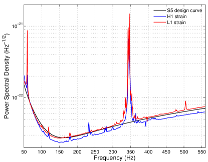
Figure 1: (colour online) LIGO S5 strain sensitivity curve (black) compared to power spectral density of both H1 (blue, lower) and L1 (red, upper) detectors during the selected 10 day data stretch, which ran from 21–31 August 2007 (GPS time 871760852–872626054).

IV.2 Pipeline

A flowchart of the multi-stage sideband pipeline is depicted in Fig. 2. After data selection, the first stage of the pipeline is the computation of the $\mathcal{F}$-statistic  Prix (2011); lal  . For the sideband search only the sky position is required at the $\mathcal{F}$-statistic stage, where the matched filter models an isolated source.

The outputs of the $\mathcal{F}$-statistic analysis are values of $2\mathcal{F}$ for each frequency bin from which the sideband algorithm then calculates the $\mathcal{C}$-statistic Sammut et al. (2014); lal . The algorithm takes values of the $\mathcal{F}$-statistic as input data and values of $P_{\text{orb}}$ and $a_{\text{\tiny{\emph{0}}}}$ as input parameters, and outputs a $\mathcal{C}$-statistic for every frequency bin in the search range (as per Eqs. 3 and 4).

The extent of the sideband template, Eq. 1, changes as a function of the search frequency $f^{\prime}$ since the number of sidebands in the template scales as $M\propto f^{\prime}$. We therefore divide the 500 Hz search band into smaller sub-bands over which we can use a single template. The sub-bands must be narrow enough, so that $f^{\prime}$ and hence $M$ do not change significantly from the lower to the upper edges of the sub-band, and wide enough to contain the entire sideband pattern for each value of $f^{\prime}$. It is preferable to generate $\mathcal{F}$-statistic data files matching these sub-bands, so that the search algorithm can call specific $\mathcal{F}$-statistic data files for each template, as opposed to each call being directed to the same large data file. However, the $\mathcal{F}$-statistic sub-bands need to be half a sideband width (or $2\pi f^{\prime}a^{\prime}/P^{\prime}$ Hz) wider on each end than the $\mathcal{C}$-statistic sub-bands in order to calculate the $\mathcal{C}$-statistic at the outer edges. For a Sco X-1 directed search, single-Hz bands are convenient; for example, even up at $f^{\prime}=1000$ Hz, the template width $4\pi f^{\prime}a/P$ is still less than 0.25 Hz.

The output of the $\mathcal{C}$-statistic is compared with a threshold value $\mathcal{C}^{*}$ chosen according to a desired false alarm rate (see Sec. IV.3 below). Any frequency bins returning $\mathcal{C}>\mathcal{C}^{*}$ are designated as candidate events and are investigated to determine whether they can be attributed to non-astrophysical origins, due to noise or detector artifacts, or to an astrophysical signal. The former are vetoed and if no candidates above $\mathcal{C}^{*}$ survive, upper limits are computed (see Sec. V.2 for more information on the veto procedure).

Figure 2: Flowchart of the search pipeline. After data selection, the $\mathcal{F}$-statistic for an isolated source is calculated in the compute $\mathcal{F}$-statistic stage with the source sky position ($\alpha$, $\delta$) as input. The output of this is then passed to the sideband search in the compute $\mathcal{C}$-statistic stage, with the binary parameters ($P_{\text{orb}}$ and $a_{\text{\tiny{\emph{0}}}}$) as input, which returns a $\mathcal{C}$-statistic. When $\mathcal{C}$ is greater than the threshold $\mathcal{C}^{*}$, the candidate is investigated as a potential signal. If no candidates survive follow-up, upper limits are presented.

IV.3 Detection Threshold

To define the threshold value $\mathcal{C}^{*}$ for a single trial we first relate it to the false alarm probability $P_{\text{a}}$, i.e. the probability that noise alone would generate a value greater than this threshold. This is given by

$$P_{\text{a}} = p(\mathcal{C}>\mathcal{C}^{*}|\text{no signal})$$ (11)

$$= 1-F(\mathcal{C}^{*},4M),$$

where $F(x,k)$ denotes the cumulative distribution function of a $\chi^{2}_{k}$ distribution evaluated at $x$ .

In the case of $N$ statistically independent trials, the false alarm probability is given by

$$P_{\text{a}|N} = 1-(1-P_{\text{a}})^{N}$$ (12)

$$= 1-\left[F(\mathcal{C}^{*},4M)\right]^{N}.$$

This can be solved for the detection threshold $\mathcal{C}^{*}_{N}$ in the case of $N$ trials, giving

$$\mathcal{C}^{*}_{N} =F^{-1}([1-P_{\text{a}|N}]^{1/N},4M),$$ (13)

where $F^{-1}$ is the inverse (not the reciprocal) of the function $F$.

The search yields a different $\mathcal{C}$-statistic for each frequency bin in the search range. If the $\mathcal{C}$-statistic values are uncorrelated, we can equate the number of independent trials with the number of independent frequency bins ($\propto T$ for each Hz band). However, due to the comb structure of the signal and template, frequencies separated by an integer number of frequency-modulated sideband spacings become correlated, since each of these values are constructed from sums of $\mathcal{F}$-statistic values containing many common values. The pattern of $M$ sidebands separated by $1/P$ Hz spans $M/P$ Hz, meaning there are $P/M$ sideband patterns per unit frequency. Hence, as an approximation, it can be assumed that within a single comb template there are $T/P$ independent $\mathcal{C}$-statistic results. The number of statistically independent trials per unit Hz is therefore given by the number of independent results in one sideband multiplied by the number of sidebands per unit frequency, i.e.

$$N \approx\frac{T}{M}.$$ (14)

This is a reduction by a factor $M$ in the number of statistically independent $\mathcal{C}$-statistic values as compared to the $\mathcal{F}$-statistic.

Using this more realistic value of $N$ provides a better analytical prediction of the detection threshold for a given $P_{\text{a}}$, which we can apply to each frequency band in our search. However, a precise determination of significance (taking into account correlations between different C-statistics among other effects) requires a numerical investigation. To factor this in, we use Monte Carlo (MC) simulations to estimate an approximate performance (or loss) factor, denoted $\kappa$. This value is estimated for a handful of 1 Hz wide frequency bands and then applied across the entire search band. For a specific 1 Hz frequency band, the complete search is repeated 100 times, each with a different realisation of Gaussian noise. The maximum $\mathcal{C}$ obtained from each run is returned, and this distribution of values allows us to estimate the value $\mathcal{C}^{*}_{MC}$ corresponding to a multi-trial false alarm probability $P_{\text{a}|N}=1\%$. For each trial frequency band, we can then estimate $\kappa$ as

$$\kappa=\frac{\mathcal{C}^{*}_{MC}-4M}{\mathcal{C}^{*}_{N}-4M}-1,$$ (15)

which can be interpreted as the fractional deviation in $\mathcal{C}$ using the number of degrees of freedom (the expected mean) as the point of reference. We assume that $\kappa$ is approximately independent of frequency (supported by Table 3) and hence use a single $\kappa$ value to represent the entire band. We incorporate this by defining an updated threshold

$$\mathcal{C}^{*}_{\kappa}=\mathcal{C}^{*}_{N}(1+\kappa)-4M\kappa$$ (16)

which now accounts for approximations in the analysis pipeline. The MC procedure was performed for 1-Hz frequency bands starting at 55, 255, and 555 Hz. Using the values returned from these bands, we take a value of $\kappa=0.3$. Table 3 lists the values of $4M$, $\mathcal{C}^{*}_{N}$, $\mathcal{C}^{*}_{MC}$ and $\kappa$ associated with each of these bands.

Table 3: Performance factor obtained from MC simulations at three different 1-Hz sub-bands. The starting frequency of the sub-band is listed in the first column. The expected C-statistic value in Gaussian noise $4M$, theoretical threshold $\mathcal{C}^{*}_{N}$, and the threshold obtained from the MC simulations $\mathcal{C}^{*}_{MC}$ are listed in the second, third and fourth columns, respectively. Performance factor $\kappa$ is listed in the last column.

sub-band (Hz)	$4M$	$\mathcal{C}^{*}_{N}$	$\mathcal{C}^{*}_{MC}$	$\kappa$
55	4028	4410	4520	0.28
255	18500	19254	19476	0.29
555	40212	41264	41578	0.30

IV.4 Upper limit calculation

If no detection candidates are identified, we define an upper limit on the gravitational wave strain $h_{\text{\tiny{\emph{0}}}}$ as the value $h_{\text{\tiny{UL}}}$ such that a predefined fraction $p_{\text{\tiny{UL}}}$ of the marginalised posterior probability distribution $p(h_{\text{\tiny{\emph{0}}}}|\mathcal{C})$ lies between 0 and $h_{\text{\tiny{UL}}}$. This value is obtained numerically for each $\mathcal{C}$-statistic by solving

$$p_{\text{\tiny{UL}}}=\int\limits_{0}^{h_{\text{\tiny{UL}}}}p(h_{\text{\tiny{\emph{0}}}}|\mathcal{C})\,\,dh_{\text{\tiny{\emph{0}}}},$$ (17)

with

$$p(h_{\text{\tiny{\emph{0}}}}|\mathcal{C})\! \propto \!\int\limits_{-\infty}^{\infty}\!dP\!\int\limits_{-\infty}^{\infty}\!da\!\int\limits_{0}^{2\pi}\!d\psi\!\int\limits_{-1}^{1}\!d\cos\iota~{}p(\mathcal{C}|\bm{\theta})\mathcal{N}(a,\Delta{a})\mathcal{N}(P,\Delta{P}),$$

and where $\mathcal{N}(\mu,\sigma)$ denotes a Gaussian (normal) distribution with mean $\mu$ and standard deviation $\sigma$. The likelihood function $p(\mathcal{C}|\bm{\theta})$ is the probability density function (pdf) of a non-central $\chi^{2}_{4M}(\lambda(\bf{\theta}))$ distribution given by

$$p(\mathcal{C}|\bm{\theta})=\frac{1}{2}\exp\left(-\frac{1}{2}\left(\mathcal{C}+\lambda\left(\bm{\theta}\right)\right)\right)\left(\frac{\mathcal{C}}{\lambda\left(\bm{\theta}\right)}\right)^{M-\frac{1}{2}}\textrm{I}_{2M-1}\left(\sqrt{\mathcal{C}\lambda\left(\bm{\theta}\right)}\right),$$ (19)

where $\textrm{I}_{\nu}(z)$ is the modified Bessel function of the first kind with order $\nu$ and argument $z$. The non-centrality parameter $\lambda(\bm{\theta)}$ is proportional to the optimal SNR (see Eq. 64 of Sammut et al. (2014)), and is a function of $\psi$, $\cos\iota$ and the mismatch in the template caused by $\Delta P$ and $\Delta a$. See Section III.5 for a description on the priors selected for $\cos\iota$ and $\psi$.

It is common practice in continuous-wave searches to compute frequentist upper limits using computationally expensive Monte Carlo simulations. The approach above allows an upper limit to be computed efficiently for each $\mathcal{C}$-statistic, since $p(h_{\text{\tiny{\emph{0}}}}|\mathcal{C})$ is calculated analytically instead of numerically and is a monotonic function of $\mathcal{C}$. We also note that for large parameter space searches the multi-trial false alarm threshold corresponds to relatively large SNR and in this regime the Bayes and frequentist upper limits have been shown to converge Röver et al. (2011).

V Results

We perform the sideband search on 10 days of LIGO S5 data spanning 21–31 August 2007 (see Fig. 1 and Sec. IV.1). The search covers the band from 50 – 550 Hz. A $\mathcal{C}$-statistic is generated for each of the $2\times 10^{6}$ frequency bins in each 1-Hz sub-band. The maximum $\mathcal{C}$-statistic from each sub-band is compared to the theoretical threshold (Eq. 16). Any $\mathcal{C}$-statistic above the threshold is classed as a detection candidate worthy of further investigation.

Without pre-processing (cleaning) of the data, non-Gaussian instrumental noise and instrumental artifacts had to be considered as potential sources for candidates. A comprehensive list of known noise lines for the S5 run, and their origins, can be found in Appendix B of Aasi et al. (2013). Candidates in sub-bands contaminated by these lines have been automatically removed. The veto described in Sec. V.2 was then applied to the remaining candidates in order to eliminate candidates that could not originate from an astrophysical signal represented by our model. This veto stage is first applied as an automated process but each candidate is also inspected manually as a verification step. If all candidates are found to be consistent with noise, no detection is claimed, and upper limits are set on the gravitational wave strain tensor amplitude $h_{0}$.

V.1 Detection candidates

The maximum $\mathcal{C}$-statistic, $\mathcal{C}_{\text{max}}$, returned from each sub-band is plotted in Fig. 3 as a function of frequency. The threshold $\mathcal{C}^{*}_{\kappa}$ for $N=T/M$ trials and $P_{\text{a}|N}=1\%$ false alarm probability is indicated by a solid black curve. Data points above this line are classed as detection candidates. Candidates in sub-bands contaminated by known instrumental noise are highlighted by green circles and henceforth discarded. The two candidates highlighted by a black star coincide with hardware-injected isolated pulsar signals “5” and “3” at $f=52.808324$ and 108.85716 Hz respectively (see Table III. in Section VI. of Aasi et al. (2013) for more details on isolated pulsar hardware injections).

The remaining candidates above the threshold are highlighted by pink squares and merit follow-up. Their frequencies $f_{\text{max}}$ and corresponding $\mathcal{C}_{\text{max}}$ and predicted threshold detection candidate $\mathcal{C}^{*}_{\kappa}$ are listed in Table 4. The detection threshold with fixed $\kappa$ varies with $f$ through the variation in the degrees of freedom in the $\mathcal{C}$ (see Sec. IV.3).

Figure 3: (colour online) Red dots indicate the maximum detection statistic for each Hz sub-band (reduced by the expected value $\text{E}[\mathcal{C}]=4M$ and normalised by the expected standard deviation $\sigma=\sqrt{8M}$) plotted as a function of frequency. The threshold value $\mathcal{C}^{*}_{N}$ for $N=T/M$ trials and $P_{\text{a}|N}=1\%$ false alarm probability is shown for comparison (solid black curve). Points exceeding the threshold are marked by green circles if they coincide with a frequency band known to be contaminated by instrumental noise lines, black stars to indicate hardware-injected isolated pulsars, or pink squares to mark candidates requiring further investigation (follow-up).

Table 4: Maximum $\mathcal{C}$-statistic from each Hz sub-band exceeding the detection threshold $\mathcal{C}^{*}_{N}$ for $N$ trials after removing isolated pulsar injections and candidates in bands contaminated by known noise lines. The first column lists the frequency $f_{max}$ at which the maximum $\mathcal{C}$-statistic $\mathcal{C}_{max}$ occurs. $\mathcal{C}_{max}$ and $\mathcal{C}^{*}_{\kappa}$ are listed in the second and third columns, respectively, for comparison.

$f_{\text{max}}$ (Hz)	$\mathcal{C}_{\text{max}}(\times 10^{3})$	$\mathcal{C}^{*}_{\kappa}(\times 10^{3})$
51.785819	5.66	4.22
53.258119	14.0	4.38
69.753009	6.88	5.6
71.879543	5.87	5.75
72.124267	6.02	5.82
73.978239	9.23	5.91
75.307963	7.90	6.06
76.186649	9.00	6.13
78.560484	12.3	6.28
80.898939	8.82	6.43
82.105904	10.2	6.58
83.585249	7.93	6.66
87.519459	12.3	6.96
99.113480	9.41	7.87
100.543741	8.72	7.94
105.277878	8.58	8.31
113.764264	9.80	8.91
114.267062	9.55	8.99
116.686578	9.29	9.14
182.150449	14.4	14.1
184.392065	14.3	14.2
244.181829	18.7	18.7
278.712575	21.3	21.2
279.738235	21.5	21.3

V.2 Noise veto

Table 5: Candidates surviving the $4M$ veto. The table lists the start frequency of the 1-Hz sub-band containing the candidate, the expected $\mathcal{C}$-statistic value $4M$, the $P_{\text{a}|N}=1\%$ threshold $\mathcal{C}^{*}_{\kappa}$, and the fraction of $\mathcal{C}$-statistics below $4M$ and above $\mathcal{C}^{*}_{\kappa}$ in the range $|f-f_{\text{max}}|<M/P$ centred at the bin $f_{\text{max}}$ returning $\mathcal{C}_{\text{max}}$. The * marks the bands containing the candidates that survive the final, manual veto.

$f_{\text{band}}$ (Hz)	$4M$	$\mathcal{C}^{*}_{\kappa}$	$\%<4M$	$\%>\mathcal{C}^{*}_{\kappa}$
69	5036	5596	15.3	52.5
71	5180	5746	1.04	1.97
105	7644	8314	1.17	4.02
116	8436	9135	1.34	1.34
184*	13356	14208	27.0	0.0204
244*	17700	18662	33.2	0.00723
278*	20164	21182	14.7	0.0365
279	20236	21255	4.71	4.5

Frequency bins coincident with signal sidebands generate $\mathcal{C}$-statistic values drawn from a $\chi^{2}_{4M}(\lambda)$ distribution, while frequency bins falling between these sidebands (the majority of bins) should follow the noise distribution $\chi^{2}_{4M}(0)$. If noise produces a spuriously loud $\mathcal{F}$-statistic in one bin, it then contributes strongly to every $\mathcal{C}$-statistic in a sideband width centred on the spurious bin, a frequency range spanning ${\sim}2M/P$, to the point where all the $\mathcal{C}$-statistics may exceed the expected mean $4M$ in this region. We can exploit this property to design a veto against candidates occurring from noise lines as follows: a candidate is vetoed as a potential astrophysical signal if the fraction of bins with $\mathcal{C}<4M$ in the range $|f-f_{\text{max}}|<M/P$ is too low, where $f_{\text{max}}$ is the frequency bin corresponding to $\mathcal{C}_{\text{max}}$. We set the minimum bin fraction to zero so as not to discard a real signal strong enough to make $\mathcal{C}>4M$ over a broad range.

Applying the veto reduces the number of candidate events from 24, shown in Table 4 to the eight listed in Table 5. The eight candidates were inspected manually to identify if the features present are consistent with a signal (see Appendix A). After manual inspection, three candidates remained, which could not be conclusively identified as a signal, but could still be expected from noise given the $1\%$ false alarm threshold set . These final three candidates were contained in the 184, 244 and 278 Hz sub-bands and were followed up in two other 10-day stretches of S5 data.

V.3 Candidate follow-up

The three remaining candidate bands were followed up by analysing two other 10-day stretches of S5 data of comparable sensitivity. A comparison of the noise spectral density of each of the 10-day stretches is displayed in Fig. 4 and the results from each of the three bands are presented in Table 6. The bands did not produce significant candidates in the two follow-up searches, indicating they were noise events. This is indicated more robustly by the combined P-values for each candidate presented at the bottom of Table 6.

All three candidates lie at the low frequency end, in the neighbourhood of known noise lines (green circles identify excluded points in Fig. 3) and may be the result of noise-floor fluctuations (caused by the non-stationarity of seismic noise, which dominates the noise-floor at low frequencies). Events such as these are expected to occur from noise in $1\%$ of cases, as defined by our false alarm threshold, and are consistent with the noise hypothesis.

Table 6: Results from candidate follow-up for each observation timespan at each Hz frequency band. The fractional percent above $\mathcal{C}^{*}_{\kappa}$ and below $4M$ are taken from the expected signal region indicated by the original candidate (which includes a sideband width centred at the candidate, plus the maximum effects of any spin wandering). The P-value is calculated for the maximum $\mathcal{C}$-statistic value in this region. A combined P-value for each candidate is displayed at the bottom of the table.

Timespan		184 Hz	244 Hz	278 Hz
21–31 Aug	% above $\mathcal{C}^{*}_{\kappa}$	0.02	0.01	0.04
2007	% below $4M$	27.02	33.22	17.72
(original)	P-value	$1.03\times 10^{-5}$	$1.12\times 10^{-5}$	$5.36\times 10^{-6}$
20 – 30 Sep	% above $\mathcal{C}^{*}_{\kappa}$	0.00	0.00	0.00
2007	% below $4M$	32.46	46.69	33.54
(follow-up)	P-value	0.92	0.27	0.36
26 May – 05 Jun	% above $\mathcal{C}^{*}_{\kappa}$	0.00	0.00	0.00
2007	% below $4M$	41.44	49.27	63.38
(follow-up)	P-value	0.50	0.47	0.15
Combined	P-value	0.99	0.75	0.60

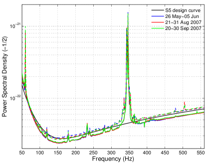
Figure 4: (colour online) LIGO S5 strain sensitivity design curve (black) compared to power spectral density of both H1 (solid, lower) and L1 (dashed, upper) detectors during the selected 10 day data stretch (red), which ran from 21–31 August 2007, and the other two stretches used for follow-up (26 May – 05 Jun 2007 indicated in blue, and 20 – 30 Sep 2007 in green).

V.4 Upper limits

Bayesian upper limits are set using Eq. 17 and an upper limit on $h_{\text{\tiny{\emph{0}}}}$ is calculated for every $\mathcal{C}$-statistic, yielding $2\times 10^{6}$ results in each 1-Hz sub-band. Figure 5 shows the upper limits for our S5 dataset (21–31 Aug 2007) combining data from the LIGO H1 and L1 detectors. The grey band in Fig. 5 stretches vertically from the minimum to the maximum upper limit in each sub-band. The solid grey curve indicates the expected value of the median $95\%$ upper limit for each sub-band given the estimated noise spectral density in the selected data. The solid black curve indicates the $95\%$ strain upper limit expected from Gaussian noise at the S5 design strain sensitivity and matches the median upper limit to within $10\%$ in well-behaved (Gaussian-like) regions. The excursions from the theoretical median, e.g. at $f\approx 350$ Hz, are noise lines, as discussed in Secs. V.1 and V.2.

Figure 5(a) shows upper limits for the standard sideband search, which adopts the electromagnetically measured values of $P_{\text{orb}}$ and $a_{\text{\tiny{\emph{0}}}}$ and flat priors on $\cos\iota$ and $\psi$ spanning their full physical range. Figure 5(b) shows upper limits for the sideband search using Gaussian priors on these angles with preferred values of $\iota=44^{\circ}\pm 6^{\circ}$ and $\psi=234^{\circ}\pm 3^{\circ}$ inferred from electromagnetic observations of the Sco X-1 jet. Section III.5 describes the two cases in more detail.

The minimum upper limit (i.e. minimised over each Hz band and shown as the lower edge of the grey region in Fig. 5) between 120 and 150 Hz, where the detector is most sensitive, equals $h_{\text{\tiny{UL}}}^{95}=6\times 10^{-25}$ with $95\%$ confidence for the standard search, and $4\times 10^{-25}$ for the angle-restricted search. The variation agrees to within $5\%$ for both configurations of the search, for which the minimum and maximum vary from ${\sim}0.5$ to ${\sim}2$ times the median, respectively.

The strain upper limit $h_{\text{\tiny{UL}}}^{95}$ for the angle-restricted search in Fig. 5(b) is ${\sim}60\%$ lower than that of the standard search in Fig. 5(a) and the variation in span between minimum and maximum within each sub-band is ${\sim}70\%$ narrower. Accurate prior knowledge of $\iota$ and $\psi$ reduces the parameter space considerably. By constructing priors from the estimated values, the upper limits improve by a factor of 1.5, though, this improvement can be applied independently of the search algorithm.

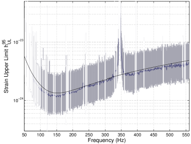
(a)

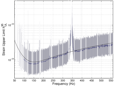
(b)

Figure 5: Gravitational wave strain $95\%$ upper limits for H1L1 data from 21–31 Aug 2007 for 5(a) the standard search with flat priors on $\cos\iota$ and $\psi$ (left panel) and 5(b) the angle-restricted search with $\iota=44^{\circ}\pm 6^{\circ}$ and $\psi=234^{\circ}\pm 4^{\circ}$ (right panel). The grey region extends from the minimum to the maximum upper limit in each 1-Hz sub-band. The median upper limit in each sub-band is indicated by a solid, thick, blue-grey curve. The expected upper limit for Gaussian noise at the S5 design sensitivity is shown for comparison (solid, thin, black curve). Whited regions of the grey band indicate bands that have been excluded (due to known contamination or vetoed out bands). No upper limits are quoted in these bands.

VI Discussion

Accretion torque balance Bildsten (1998) implies an upper limit $h_{\text{\tiny{\emph{0}}}}^{\text{EQ}}\leqslant 7\times 10^{-26}$ at 150 Hz for Sco X-1 (see Eq. 5). This sets the maximum expected strain at ${\sim}6$ times lower than our angle-restricted upper limit ($4\times 10^{-25}$), assuming spin equilibrium as implied by torque balance. This is a conservative limit. Taking the accretion-torque lever arm as the Alfvén radius instead of the neutron star radius increases $h_{\text{\tiny{\emph{0}}}}^{\text{EQ}}$ by a factor of a few, as does relaxing the equilibrium assumption. Torque balance may or may not apply if radiative processes modify the inner edge of the accretion disk Patruno et al. (2012).

The sideband search upper limit can be used to place an upper limit on the neutron star ellipticity $\epsilon$. We can express the ellipticity $\epsilon$ in terms of $h_{\text{\tiny{\emph{0}}}}$ by

$$\epsilon = \frac{5c^{4}}{8\pi G}\frac{D}{MR^{2}}\frac{h_{\text{\tiny{\emph{0}}}}}{{\nu_{\text{s}}}^{2}},$$ (20)

where $M$, $R$, and $\nu_{\text{s}}$ are the mass, radius and spin frequency of the star, respectively, and $D$ is its distance from Earth Jaranowski et al. (1998). Using fiducial values $M=1.4M_{\odot}$ and $R=10$ km and assuming $f=2\nu_{\text{s}}$ (i.e. the principal axis of inertia is perpendicular to the rotation axis), the upper limit $\epsilon_{\text{\tiny{UL}}}$ for Sco X-1 can be expressed as

$$\epsilon_{\text{\tiny{UL}}}\leqslant 5\times 10^{-4}{\left(\frac{h_{\text{\tiny{UL}}}}{4\times 10^{-25}}\right)}{\left(\frac{f}{150\text{ Hz}}\right)}^{-2}\left(\frac{D}{2.8\text{ kpc}}\right).$$ (21)

This is well above the ellipticities predicted by most theoretical quadrupole generating mechanisms. Thermocompositional mountains have $\epsilon\approx 9\times 10^{-6}$ for $\lesssim 5\%$ lateral temperature variations in a single electron capture layer in the deep inner crust or $0.5\%$ lateral variations in charge-to-mass ratio Ushomirsky et al. (2000). Magnetic mountain ellipticities vary with the equation of state (EOS). For a pre-accretion magnetic field of $10^{12.5}$ G, one finds $\epsilon\approx 2\times 10^{-5}$ and $\epsilon\approx 6\times 10^{-8}$ for isothermal and relativistic-degenerate-electron matter respectively Vigelius and Melatos (2009); Priymak et al. (2011). Equivalent ellipticities of $\epsilon{\sim}10^{-6}$ are achievable by r-mode amplitudes of a few times $10^{-4}$ Owen et al. (1998); Bondarescu et al. (2007); Abadie et al. (2010). Our upper limit approaches the ellipticity predicted for certain exotic equations of state Johnson-McDaniel and Owen (2013); Glampedakis et al. (2012); Owen (2005).

The sideband search presented here is restricted to $T_{\text{obs}}=10$ days due to current limitations in the understanding of spin wandering, i.e. the fluctuations in the neutron star spin frequency due to a time varying accretion torque. The 10-day restriction follows from the accretion torque fluctuations inferred from the observed X-ray flux variability, as discussed in Section IV. B. in Sammut et al. (2014). Improvements in understanding of this feature of phase evolution and how to effectively account for it could allow us to lengthen $T_{\text{obs}}$ and hence increase the sensitivity of the search according to $h_{\text{\tiny{\emph{0}}}}\propto T_{\text{obs}}^{-1/2}$. Pending that, results from multiple 10-day stretches could be incoherently combined, however, the unknown change in frequency between observations must be accounted for. Sensitivity would also increase if data from additional comparably sensitive detectors are included, since $h_{\text{\tiny{\emph{0}}}}\propto N_{\text{det}}^{-1/2}$, where $N_{\text{det}}$ is the number of detectors, without significantly increasing the computational cost Prix (2007).

VII Conclusion

We present results of the sideband search for the candidate gravitational wave source in the LMXB Sco X-1. No evidence was found to support detection of a signal with the expected waveform. We report $95\%$ upper limits on the gravitational wave strain $h_{\text{\tiny{UL}}}^{95}$ for frequencies $50\leqslant f\leqslant 550$ Hz. The tightest upper limit, obtained when the inclination $\iota$ and gravitational wave polarisation $\psi$ are known from electromagnetic measurements, is given by $h_{\text{\tiny{UL}}}^{95}\approx 4\times 10^{-25}$. It is achieved for $120\leqslant f\leqslant 150$ Hz, where the detector is most sensitive. The minimum upper limit for the standard search, which assumes no knowledge of source orientation (i.e. flat priors on $\iota$ and $\psi$), is $h_{\text{\tiny{UL}}}^{95}=6\times 10^{-25}$ in this frequency range. The median upper limit in each 1-Hz sub-band provides a robust and representative estimate of the sensitivity of the search. The median upper limit at 150 Hz was $1.3\times 10^{-24}$ and $8\times 10^{-25}$ for the standard and angle-restricted searches respectively.

The results improve on upper limits set by previous searches directed at Sco X-1 and motivates future development of the search. The improvement in results is achieved using only a 10-day coherent observation time, and with modest computational expense. Previously, using roughly one year of coincident S5 data, the radiometer search returned a median $90\%$ root-mean-square strain upper limit of $h_{\text{rms}}^{90}\approx 7\times 10^{-25}$ at 150 Hz Abadie et al. (2011), which converts to $h_{0}^{95}\approx 2\times 10^{-24}$ str ; rad ; Messenger (2010).

The first all-sky search for continuous gravitational wave sources in binary systems using the TwoSpect algorithm has recently reported results using ${\sim}1.25$ years of S6 data from the LIGO and VIRGO detectors  Goetz and Riles (2011); Aasi et al. (2014). Results of an adapted version of the analysis directed at Sco X-1 assuming the electromagnetically measured values of $P_{\text{orb}}$ and $a_{\text{\tiny{\emph{0}}}}$ was also reported together with the results of the all-sky search. Results of this analysis are comparable in sensitivity to the sideband search. Results for the Sco X-1 directed search were restricted to the frequency band $20\leqslant f\leqslant 57.25$ Hz due to limitations resulting from 1800-s SFTs.

We have shown that this low computational cost, proof-of-principle analysis, applied to only 10 days of data, has provided the most sensitive search for gravitational waves from Sco X-1. The computational efficiency and relative sensitivity of this analysis over relatively short coherent time-spans makes it an appealing search to run as a first pass in the coming second-generation gravitational wave detector era. Running in low-latency with the capability of providing updated results on a daily basis for multiple LMXB systems would give the first results from continuous wave searches for sources in known binary systems. With a factor 10 improvement expected from advanced detectors, and the sensitivity of semi-coherent searches improving with the fourth root of the number of segments and, for our search, also with the square root of the number of detectors, we can hope for up to a factor ${\sim}$30 improvement for a year long analysis with 3 advanced detectors. This would place the sideband search sensitivity within reach of the torque-balance limit estimate of the Sco X-1 strain (Eq.  5) in the most sensitive frequency range, around 150 Hz. However, the effects of spin wandering will undoubtedly weaken our search and impose a larger trials factor to our detection statistic, therefore increasing our detection threshold. Efficient analysis methods that address spin wandering issues to allow longer coherent observations or combine results from separate observations should improve the sensitivity of the search, enhancing its capability in this exciting era.

Appendix A Manual veto

The eight candidates surviving the automated $4M$ veto, listed in Table 5, were followed up manually. The manual follow-up of these candidates is presented here in more detail. Both the automated and manual veto stages were tested on software injected signals and simulated Gaussian noise to ensure signals were not accidentally vetoed. The tests showed that the vetoes are conservative.

Figures 6, 7 and 8 display the output ($\mathcal{F}$-statistic in magenta and $\mathcal{C}$-statistic in cyan) for the 1-Hz sub-bands containing the candidates surviving the $4M$ veto. The frequency range used for the veto is highlighted in blue in each plot. Some $\mathcal{C}$-statistics in this region are further highlighted in red if they exceed the threshold $\mathcal{C}^{*}_{\kappa}$ or magenta if they fall below $4M$. The expected values ($\mathcal{F}=4$ and $\mathcal{C}=4M$) are indicated by solid black-dashed horizontal lines. The threshold $\mathcal{C}^{*}_{\kappa}$ is indicated by a green horizontal dashed line in each of the $\mathcal{C}$-statistic plots.

Figure 6 displays the output of the sub-band starting at 69 Hz, containing a candidate judged to arise from a noise line. The line is clearly evident in the $\mathcal{F}$-statistic (left hand panel). The sideband signal targeted by this search will be split over many $\mathcal{F}$-statistic bins due to the modulation caused by the motion of the source in its binary orbit. The signal is not expected to be contained in a single bin. The veto should automatically rule out single-bin candidates such as this one, however the veto fails to reject this candidate because $f_{\text{max}}$ (where the veto band is centered) falls closer to one end of the contaminated region rather than the centre. In this special scenario the veto picks up several bins with $\mathcal{C}<4M$ from just outside the contaminated region (where the noise is “normal”) so the candidate survives. Visual inspection is important in these cases and shows clearly that the candidate could not result from a signal.

Figure 7 shows the $\mathcal{C}$-statistic output for the other candidate sub-bands attributed to noise. The features visible in the $\mathcal{C}$-statistic can be ruled out as originating from an astrophysical signal since the fraction of bins above $4M$ is too large compared to what would be expected from such a signal with the same apparent SNR. We would expect the frequency bins in between sidebands to drop down to values of $\mathcal{C}{\sim}4M$, resulting in a consistent noise floor even around the candidate “peak”. The elevated noise floor around the peaks is not consistent with an expected signal. Similar features can be seen in each of the sub-bands starting at 71, 105, 116 and 279 Hz.

Figure 8 presents the candidates in the 184, 244 and 278 Hz sub-bands, which are consistent with false alarms expected from noise. The candidate in the 184 Hz sub-band has a healthy fraction ($26\%$) of bins with $\mathcal{C}<4M$ and resembles the filled dome with consistent noise floor expected from a signal (unlike the examples in Fig. 7), although it is slightly pointier. At $f=244$ Hz, $33\%$ of bins have $\mathcal{C}<4M$ but the $\mathcal{C}$-statistic pattern is multimodal and less characteristic of a signal. The candidate peak is comparable in amplitude to several other fluctuations within the sub-band, possibly indicating a contaminated (non-Gaussian) noise-floor. Similar remarks apply to $f=278$ Hz, especially consideration of the noise-floor fluctuations. Additionally, the candidate at 278 Hz also coincides with a strong, single-bin spike in the $\mathcal{F}$-statistic at 278.7 Hz.

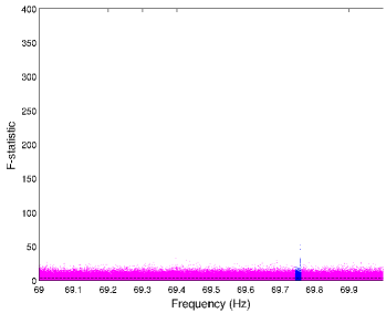
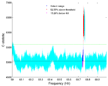
Figure 6: (colour online) $\mathcal{F}$-statistic (left, magenta) and $\mathcal{C}$-statistic (right, cyan) versus frequency for Hz sub-band beginning at 69 Hz containing a candidate surviving the $4M$ veto which is attributed to a noise line. The frequency range used to determine the veto is highlighted (blue points). Points in the $\mathcal{C}$-statistic veto region are further highlighted (in red) if they exceed the threshold $\mathcal{C}^{*}_{\kappa}$ and (in pink) if they fall below the expectation value of the noise $4M$. The horizontal black dashed line indicates the expected value for noise ($\mathcal{F}=4$, $\mathcal{C}=4M$). The threshold value $\mathcal{C}^{*}_{\kappa}$ is also indicated on the $\mathcal{C}$-statistic plots by a horizontal green dashed line. The percentage of $\mathcal{C}$-statistics falling above $\mathcal{C}^{*}_{\kappa}$ or below $4M$ is quoted in the legend in each $\mathcal{C}$-statistic panel.

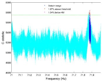
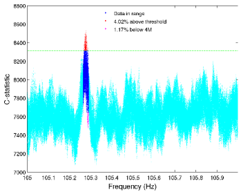
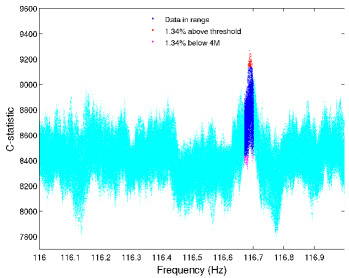
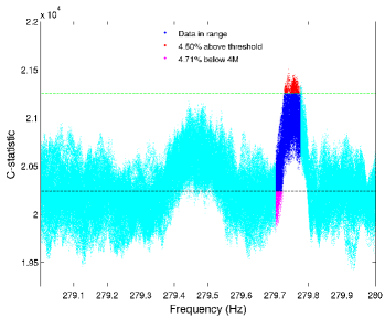
Figure 7: (colour online) As for Figure 6 but for sub-bands beginning at 71, 105, 116 and 279 Hz containing candidates surviving the $4M$ veto with features not consistent with a signal, which are attributed to noise.

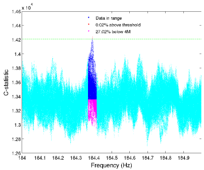
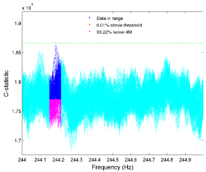
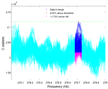
Figure 8: (colour online) As for Figure 6 but for sub-bands beginning at 184, 244 and 278 Hz that survive the $4M$ veto which are consistent with false alarms expected from noise.