The purpose of this paper is to implement a random death process into a persistent random walk model which produces subballistic superdiffusion (Lévy walk). We develop a Markovian model of cell motility with the extra residence variable $\tau.$ The model involves a switching mechanism for cell velocity with dependence of switching rates on $\tau$. This dependence generates intermediate subballistic superdiffusion. We derive master equations for the cell densities with the generalized switching terms involving the tempered fractional material derivatives. We show that the random death of cells has an important implication for the transport process through tempering of superdiffusive process. In the long-time limit we write stationary master equations in terms of exponentially truncated fractional derivatives in which the rate of death plays the role of tempering of a Lévy jump distribution. We find the upper and  lower bounds for the stationary profiles corresponding to the ballistic transport and diffusion with the death rate dependent diffusion coefficient. Monte Carlo simulations confirm these bounds.

1 Introduction

Cell motility is an important factor in embryonic morphogenesis, wound healing, cancer proliferation, and many other physiological and pathological processes [1]. The microscopic theory of the cell migration is based on various random walk models [2]. Most theoretical studies of cell motility deal with Markovian random walks [3, 4, 5]. However, the experimental analysis of the trajectories of cells shows that they might exhibit non-Markovian superdiffusive dynamics [6, 7, 8]. It has been found recently that cancer cells motility is superdiffusive [9, 10].

Several techniques are available to obtain a superdiffusion including the continuous time random walk (CTRW) [11, 12, 13], generalization of the Markovian persistent random walk [14, 15, 16], stochastic differential equations [17], a fractional Klein–Kramers equation [7, 18], non-Markovian switching model [19]. The CTRW model [11, 12, 13] for superdiffusion involves the joint probability density function (PDF) $\Phi(\tau,r)$ for a waiting time $\tau$ and a displacement (jump) $r$. One has to assume that the waiting time and displacement are correlated. For example, $\Phi(\tau,r)$ $=\delta(\tau-|r|/v)w(r)$ with $w(r)$ $\sim|r|^{-\mu}$ ($2<\mu<3)$ as $r\rightarrow\infty$ corresponds to the Lévy walk for which the particle moves with a constant speed $v$, and the waiting time $\tau$ depends on the displacement. The mean-square displacement for the Lévy walk is $\mathbb{E}X^{2}(t)\sim t^{4-\mu}$ (superdiffusion). Another way to obtain a superdiffusive bevaviour is a two-state model with power law sojourn time densities as the generalization of correlated random walk involving two velocities [14, 15, 16]. One can  also start with the stochastic differential equation for the position of particle $X(t):$ $\dot{X}(t)=v(t),$ where the velocity $v(t)$ is a dichotomous stationary random process with zero mean which takes two values $V$ and $-V$ [17]. One can obtain a superdiffusive increase of the mean squared displacement in time by using a fractional Klein–Kramers equation for the probability density function for the position and velocity of cells [7, 18]. This equation generates power law velocity autocorrelation, $C_{v}(t)\sim E_{\mu}\left[-\left(\frac{t}{\tau_{0}}\right)^{\mu}\right],$ involving the Mittag-Leffler function $E_{\mu}$ which explains the superdiffusive behaviour. In [19] the authors proposed a Markov model with an ergodic two-component switching mechanism that dynamically generates anomalous superdiffusion.

In this paper we address the problem of the mesoscopic description of transport of cells performing superdiffusion with the random death process. One of the main challenges is how to implement the death process into a non-Markovian transport processes governed by a persistent random walk with power law velocity autocovariance. We do not impose the power-law velocity correlations at the very beginning. Rather, this correlation function is dynamically generated by internal switching involving the age dependent switching rate. There exist several approaches and techniques to deal with the problem of persistent random walk with reactions [20, 21, 22, 23, 24, 25]. However these works are concerned only with a Markovian switching between two states. Our main objective here is to incorporate the death process into non-Markovian superdiffusive transport equations which is still an open problem. We show that the random death of cells has an important implication for the transport process through tempering of superdiffusive process.

2 Persistent random walk model involving superdiffusion

The basic setting of our model is as follows. The cell moves on the right and left with the constant velocity $v$ and turns with the rate $\gamma(\tau)$. The essential feature of our model is that the switching rate $\gamma(\tau)$ depends upon the time which the cell has spent moving in one direction [3]. We suggest that the switching rate $\gamma(\tau)$ is a decreasing function of residence time $\tau$ (negative aging). This rate describes the anomalous persistence of cell motility: the longer cell moves in one direction, the smaller the switching probability to another direction becomes. Keeping in mind a superdiffusive movement of the cancer cells [9, 10], we consider the inhibition of cell proliferation by anticancer therapeutic agents [26]. To describe this inhibition we consider the random death process assuming that during a small time interval $\left(t,t+\Delta t\right)$ each cell has a chance $\theta\Delta t+o(\Delta t)$ of dying, where $\theta$ is the constant death rate. In what follows we show that the governing equations for the cells densities involve a non-trivial combination of transport and death kinetic terms because of memory effects [20, 27, 28, 29, 30].

Let us define the mean density of cells, $n_{+}(x,t,\tau),$ at point $x$ and time $t$ that move in the right direction with constant velocity $v$ during time $\tau$ since the last switching. The mean density $n_{-}(x,t,\tau)$ corresponds to the cell movement on the left. The balance equations for both densities $n_{+}(x,t,\tau)$ and $n_{-}(x,t,\tau)$ can be written as

$$\frac{\partial n_{+}}{\partial t}+v\frac{\partial n_{+}}{\partial x}+\frac{\partial n_{+}}{\partial\tau}=-\gamma(\tau)n_{+}-\theta n_{+},$$ (1)

$$\frac{\partial n_{-}}{\partial t}-v\frac{\partial n_{-}}{\partial x}+\frac{\partial n_{-}}{\partial\tau}=-\gamma(\tau)n_{-}-\theta n_{-},$$ (2)

where $\gamma(\tau)$ is the switching rate and $\theta$ is the constant death rate. We assume that at the initial time $t=0$ all cells just start to move such that

$$n_{\pm}(x,0,\tau)=\rho_{\pm}^{0}(x)\delta(\tau),$$ (3)

where $\rho_{+}^{0}(x)$ and $\rho_{-}^{0}(x)$ are the initial densities.

Our aim is to derive the master equations for the mean density of cells moving right, $\rho_{+}(x,t),$ and the mean density of cells moving left, $\rho_{-}(x,t)$ defined as

$$\rho_{\pm}(x,t)=\int_{0}^{t^{+}}n_{\pm}(x,t,\tau)d\tau,$$ (4)

where the upper limit of $t^{+}$ is shorthand notation for $\lim_{\varepsilon\rightarrow 0}\int_{0}^{t+\varepsilon}.$ This limit emphasizes that singularity located at $\tau=t$ is entirely captured by the integration with respect to the residence variable $\tau$. Boundary conditions at $\tau=0$ are

$$n_{\pm}(x,t,0)=\int_{0}^{t^{+}}\gamma(\tau)n_{\mp}(x,t,\tau)d\tau.$$ (5)

The main advantage of the system (1) and (2) together with (3) and (5) is that it is Markovian one. From this system one can obtain various non-Markovian models including subdiffusive and superdiffusive fractional equations. It can be done by eliminating the residence time variable $\tau$ as in (4) and introducing particular models for the switching rate $\gamma(\tau)$.

2.1 Switching rate $\gamma(\tau)$

One of the main purposes of this paper is to explore the anomalous case when the switching rate $\gamma(\tau)$ is inversely proportional to the residence time $\tau$ (negative aging). This rate describes the anomalous persistence of a random walk: the longer a cell moves in a particular direction without switching, the smaller the probability of switching to another direction becomes. Here we consider two cases involving the Mittag-Leffler function and Pareto distribution.

Case 1. We make use of the following switching rate [31]

$$\gamma(\tau)=-\frac{\dot{\Psi}\left(\tau\right)}{\Psi\left(\tau\right)}$$ (6)

with the survival probability [32]

$$\Psi\left(\tau\right)=E_{\mu}\left[-\left(\frac{\tau}{\tau_{0}}\right)^{\mu}\right],\ 0<\mu<1,$$ (7)

where $\tau_{0}$ is the time constant, $E_{\mu}\left[z\right]$ is the Mittag-Leffler function.

Case 2. We employ the explicit expression for the switching rate as [15, 30] 

$$\gamma(\tau)=\frac{\mu}{\tau_{0}+\tau},\ 0<\mu<2.$$ (8)

This assumption together with (6) leads to a survival function $\Psi(\tau)$ that has a power law dependence (Pareto distribution)

$$\Psi(\tau)=\left[\frac{\tau_{0}}{\tau_{0}+\tau}\right]^{\mu}.$$ (9)

Our next step is to obtain the non-Markovian equations for $\rho_{+}(x,t)$ and $\rho_{-}(x,t)$ by eliminating the residence time variable $\tau$ (see (4)).

3 Non-Markovian master equations for $\rho_{+}(x,t)$ and $\rho_{-}(x,t)$

The aim now is to find equations for $\rho_{+}(x,t)$ and $\rho_{-}(x,t)$ by solving the partial differential equations (1) and (2) together with the boundary condition (5) at $\tau=0$ and initial condition (3) at $t=0$. By using the method of characteristics we find for $\tau<t$

$$n_{\pm}(x,t,\tau)=n_{\pm}(x\mp v\tau,t-\tau,0)e^{-\int_{0}^{\tau}\gamma(u)du}e^{-\theta\tau}.$$ (10)

It is convenient to use the survival function from (6)

$$\Psi(\tau)=e^{-\int_{0}^{\tau}\gamma(u)du}.$$ (11)

and the fluxes between two states (switching terms) $i_{+}(x,t)$ and $i_{-}(x,t):$

$$i_{\pm}(x,t)=\int_{0}^{t^{+}}\gamma(\tau)n_{\pm}(x,t,\tau)d\tau.$$ (12)

We notice that  $n_{+}(x,t,0)=i_{-}(x,t)$ and $n_{-}(x,t,0)=i_{+}(x,t),$ so the formula (10) can be rewritten as

$$n_{\pm}(x,t,\tau)=i_{\mp}(x\mp v\tau,t-\tau)\Psi(\tau)e^{-\theta\tau}.$$ (13)

This formula has a very simple meaning. For example, the density $n_{+}(x,t,\tau)$ gives the number of cells at point $x$ and time $t$ moving in the right direction during time $\tau$ as a result of the following process. The first factor in the RHS of (13), $i_{-}(x-v\tau,t-\tau),$ gives the number of cells that switch their velocity from $-v$ to $v$ at the point $\ x-v\tau$ at the time $t-\tau$ and survive during movement time $\tau$ due to random switching described by $\Psi(\tau)$ and the death process described by $e^{-\theta\tau}.$

The balance equations for the unstructured density $\rho_{\pm}(x,t)=\int_{0}^{t^{+}}n_{+}(x,t,\tau)d\tau$ can be found by differentiating (4) together with (13) with respect to time $t$ or by using the Fourier-Laplace transform technique (see Appendix 1, part (B)). We obtain

$$\frac{\partial\rho_{+}}{\partial t}+v\frac{\partial\rho_{+}}{\partial x}=-i_{+}(x,t)+i_{-}(x,t)-\theta\rho_{+},$$ (14)

$$\frac{\partial\rho_{-}}{\partial t}-v\frac{\partial\rho_{-}}{\partial x}=i_{+}(x,t)-i_{-}(x,t)-\theta\rho_{-}.$$ (15)

These two equations have a similar structure to the standard model for a persistent random walk with reactions [20, 21, 22, 23, 24], but the switching terms $i_{+}(x,t)$ and $i_{-}(x,t)$ are essentially different from the simple Markovian terms $\gamma\rho_{+}$ and $\gamma\rho_{-}:$

$$i_{+}(x,t)=\int_{0}^{t}K(t-\tau)\rho_{+}(x-v(t-\tau),\tau)e^{-\theta(t-\tau)}d\tau,$$ (16)

$$i_{-}(x,t)=\int_{0}^{t}K(t-\tau)\rho_{-}(x+v(t-\tau),\tau)e^{-\theta(t-\tau)}d\tau.$$ (17)

Here $K(\tau)$ is the memory kernel determined by its Laplace transform [36]

$$\hat{K}(s)=\frac{\hat{\psi}(s)}{\hat{\Psi}(s)},$$ (18)

where $\hat{\psi}(s)$ and $\hat{\Psi}(s)$ are the Laplace transforms of the residence time density $\psi(\tau)=-d\Psi/d\tau$ and the survival function $\Psi(\tau).$ One can see that $i_{+}(x,t)$ and $i_{-}(x,t)$ depend on the death rate $\theta$ and transport process involving velocity $v.$ This is a non-Markovian effect [33, 34, 35]. To obtain (16) and (17), we use the Fourier-Laplace transform

$$\tilde{\imath}_{\pm}(k,s)=\int_{\mathbb{R}}\int_{0}^{t}i_{\pm}(x,t)e^{ikx-st}dtdx,$$ (19)

$$\tilde{\rho}_{\pm}(k,s)=\int_{\mathbb{R}}\int_{0}^{t}\rho_{\pm}(x,t)e^{ikx-st}dtdx.$$ (20)

We find (see Appendix 1, part (A))

$$\tilde{\imath}_{\pm}(k,s)=\frac{\hat{\psi}(s\mp ikv+\theta)}{\hat{\Psi}(s\mp ikv+\theta)}\tilde{\rho}_{\pm}(k,s).$$ (21)

Inverse Fourier-Laplace transform gives the explicit expressions for the switching terms $i_{+}(x,t)$ and $i_{-}(x,t)$ in terms of the unstructured densities $\rho_{+}(x,t)$ and $\rho_{-}(x,t).$

If we introduce the notations

$$\hat{\Psi}_{\theta}^{\pm}=\hat{\Psi}(s\pm ikv+\theta),\ \hat{\psi}_{\theta}^{\pm}=\hat{\psi}(s\pm ikv+\theta),$$

then the Fourier-Laplace transform of the total density $\rho(x,t)=\rho_{+}(x,t)+\rho_{-}(x,t)$ can be written as (see Appendix 1, part (C))

$$\tilde{\rho}(k,s)=\frac{\rho_{+}^{0}(k)\left[\hat{\Psi}_{\theta}^{-}+\hat{\Psi}_{\theta}^{+}\hat{\psi}_{\theta}^{-}\right]+\rho_{-}^{0}(k)\left[\hat{\Psi}_{\theta}^{+}+\hat{\Psi}_{\theta}^{-}\hat{\psi}_{\theta}^{+}\right]}{1-\hat{\psi}_{\theta}^{+}\hat{\psi}_{\theta}^{-}},$$ (22)

where $\rho_{\pm}^{0}(k)=\int_{\mathbb{R}}\rho_{\pm}^{0}(x)e^{ikx}dx.$

3.1 Markovian two-state model

If the switching rate $\gamma(\tau)$ is constant, it corresponds to the exponential survival function $\Psi(\tau)=e^{-\gamma\tau}$ for which $\hat{K}(s)=\gamma$ and $K(\tau)=\gamma\delta\left(\tau\right)$. In this case (14) and (15) can be reduced to a classical two-state Markovian model for the density of cells moving right, $\rho_{+}(x,t),$ and the density of cells moving left, $\rho_{-}(x,t):$

$$\frac{\partial\rho_{+}}{\partial t}+v\frac{\partial\rho_{+}}{\partial x}=-\gamma\left(\rho_{+}-\rho_{-}\right)-\theta\rho_{+},$$ (23)

$$\frac{\partial\rho_{-}}{\partial t}-v\frac{\partial\rho_{-}}{\partial x}=-\gamma\left(\rho_{+}-\rho_{-}\right)-\theta\rho_{-}.$$ (24)

When $\theta=0,$ the model is well known as the persistent random walk or correlated random walk which was analyzed in [38, 39]. The whole idea of this random walk model was to remedy the unphysical property of Brownian motion of infinite propagation. Two equations (23) and (24) can be rewritten as a telegraph equation for the total density $\rho(x,t)=\rho_{-}(x,t)+\rho_{+}(x,t)$. This model covers the ballistic motion and the standard diffusive motion in the limit $v\rightarrow\infty$ and $\gamma\rightarrow\infty$ such that $v^{2}/\gamma$ remains constant. The Markovian model has been studied thoroughly and all details can be found in [20, 21, 22, 23, 24]. We should mention that relatively simple extension of the two-state Markovian dynamical system (23) and (24) is the non-Markovian model with the waiting time PDF of the form

$$\psi\left(\tau\right)=\beta^{2}\tau e^{-\beta\tau}.$$

In this case, the Laplace transforms are

$$\hat{\psi}(s)=\frac{\beta^{2}}{\left(\beta+s\right)^{2}},\quad\hat{K}(s)=\frac{s\hat{\psi}(s)}{1-\hat{\psi}(s)}=\frac{\beta^{2}}{2\beta+s}.$$

The memory kernel in (16) and (17) has an exponential form

$$K\left(\tau\right)=\beta^{2}e^{-2\beta\tau}.$$

Non-Markovian random motions of particles with velocities alternating at Erlang-distributed and gamma-distributed random times have been considered in [40, 41]. In this paper we will focus on the anomalous case involving cells velocities alternating at power-law distributed random times [14, 15, 16].

3.2 Non-Markovian model involving anomalous switching

Let us consider two anomalous cases when the switching rate $\gamma(\tau)$ (6) is inversely proportional to the residence time $\tau$.

Case 1. The Laplace transforms of the survival function $\Psi\left(\tau\right)=E_{\mu}\left[-\left(\frac{\tau}{\tau_{0}}\right)^{\mu}\right]\$and $\psi(\tau)=-d\Psi\left(\tau\right)/d\tau$ are

$$\hat{\Psi}\left(s\right)=\frac{\tau_{0}^{\mu}s^{\mu-1}}{1+\left(s\tau_{0}\right)^{\mu}},\quad\ \hat{\psi}\left(s\right)=\frac{1}{1+\left(s\tau_{0}\right)^{\mu}}.$$ (25)

The Laplace transform of the memory kernel $K\left(\tau\right)$ is

$$\hat{K}\left(s\right)=\frac{s^{1-\mu}}{\tau_{0}^{\mu}}.$$ (26)

Case 2. The survival function $\Psi(\tau)$ has a Pareto distribution (9) and corresponding waiting time PDF $\psi(\tau)$ is

$$\psi(\tau)=\frac{\mu\tau_{0}^{\mu}}{(\tau_{0}+\tau)^{1+\mu}}.$$ (27)

When $0<\mu<1$, the asymptotic approximation for the Laplace transform $\hat{\psi}\left(s\right)$ can be found from the Tauberian theorem [37]

$$\hat{\psi}\left(s\right)\simeq 1-\Gamma(1-\mu)\tau_{0}{}^{\mu}s^{\mu},\qquad s\rightarrow 0.$$ (28)

The Laplace transform of memory kernel $K(\tau)$ can be written approximately as

$$\hat{K}\left(s\right)\simeq\frac{s^{1-\mu}}{\Gamma(1-\mu)\tau_{0}^{\mu}}.$$ (29)

Note that the only difference between (26) (case 1) and (29) (case 2) is the $\Gamma(1-\mu)$ in the denominator in (29).

3.3 Tempered fractional material derivatives

In the anomalous case the switching terms (16) and (17) can be written in terms of tempered fractional material derivatives. Using (21) and (26) we write the Fourier-Laplace transforms of $i_{+}(x,t)$ and $i_{-}(x,t)$ as

$$\tilde{\imath}_{\pm}(k,s)=\tau_{0}^{-\mu}(s\mp ikv+\theta)^{1-\mu}\tilde{\rho}_{\pm}(k,s).$$ (30)

We define the tempered fractional material derivatives $\left(\frac{\partial}{\partial t}\pm v\frac{\partial}{\partial x}+\theta\right)^{1-\mu}$ of order $1-\mu$ by their Fourier-Laplace transforms

$$\mathcal{LF}\left\{\left(\frac{\partial}{\partial t}\pm v\frac{\partial}{\partial x}+\theta\right)^{1-\mu}\rho\right\}=(s\pm ikv+\theta)^{1-\mu}\tilde{\rho},\quad 0<\mu<1.$$ (31)

Note that fractional material derivatives with the factor $(s\pm ik)^{1-\mu}$ have been introduced in [16]. Evolution equations for anomalous diffusion involving coupled space-time fractional derivative operators involving the Fourier-Laplace symbols like $(s+ik)^{\beta},$ $(s+k^{2})^{\beta},$ etc. have been considered in [42, 43, 44]. Here we have the tempered fractional derivative operator (31) that involves both the advective transport  and the death rate $\theta.$ The latter plays the role of tempering parameter because $(s\pm ikv+\theta)^{1-\mu}$ has a finite limit $\theta^{1-\mu}$ as $s\rightarrow 0$ and $k\rightarrow 0$. We represent the anomalous switching terms as

$$i_{\pm}(x,t)=\tau_{0}^{-\mu}\left(\frac{\partial}{\partial t}\mp v\frac{\partial}{\partial x}+\theta\right)^{1-\mu}\rho_{\pm},\quad 0<\mu<1.$$

The master equations (14) and (15) can be rewritten as

$$\frac{\partial\rho_{+}}{\partial t}+v\frac{\partial\rho_{+}}{\partial x}=-\tau_{0}^{-\mu}\left(\frac{\partial}{\partial t}-v\frac{\partial}{\partial x}+\theta\right)^{1-\mu}\rho_{+}+\tau_{0}^{-\mu}\left(\frac{\partial}{\partial t}+v\frac{\partial}{\partial x}+\theta\right)^{1-\mu}\rho_{-}-\theta\rho_{+},$$ (32)

$$\frac{\partial\rho_{-}}{\partial t}-v\frac{\partial\rho_{-}}{\partial x}=-\tau_{0}^{-\mu}\left(\frac{\partial}{\partial t}+v\frac{\partial}{\partial x}+\theta\right)^{1-\mu}\rho_{-}+\tau_{0}^{-\mu}\left(\frac{\partial}{\partial t}-v\frac{\partial}{\partial x}+\theta\right)^{1-\mu}\rho_{+}-\theta\rho_{-}.$$ (33)

Note that when $\theta=0$ these equations describe a very strong persistence in a particular direction. For the symmetrical initial conditions

$$\rho_{+}^{0}(x)=\frac{1}{2}\delta\left(x\right),\quad\rho_{-}^{0}(x)=\frac{1}{2}\delta\left(x\right)$$

for which $\mathbb{E}\left\{x(t)\right\}=0$, the mean squared displacement $\mathbb{E}\left\{x^{2}(t)\right\}$ exhibits ballistic behaviour [14, 15, 16]:

$$\mathbb{E}\left\{x^{2}(t)\right\}\simeq t^{2}.$$

However, if all cells at $t=0$ start to move to the right with the velocity $v$ from the point $x=0:$

$$\rho_{+}^{0}(x)=\delta\left(x\right),\quad\rho_{-}^{0}(x)=0,$$

then (see Appendix 2) the first moment $\mathbb{E}\left\{x(t)\right\}$ is

$$\mathbb{E}\left\{x(t)\right\}\simeq\frac{v\tau_{0}^{\mu}}{2}t^{1-\mu}.$$

The subballistic behaviour of $\mathbb{E}\left\{x(t)\right\}$ was obtained in [18] for the fractional Kramers equation.

In the large scale limit $k\rightarrow 0,$ we expand $(s+\theta+ikv)^{1-\mu}=\allowbreak\left(s+\theta\right)^{1-\mu}+ikv\left(1-\mu\right)\left(s+\theta\right)^{-\mu}+o(k)$ and obtain from (30)

$$\tilde{\imath}_{+}(k,s)=\tau_{0}^{-\mu}\left[(s+\theta)^{1-\mu}-ikv\left(1-\mu\right)\left(s+\theta\right)^{-\mu}\right]\tilde{\rho}_{+},$$ (34)

$$\tilde{\imath}_{-}(k,s)=\tau_{0}^{-\mu}\left[(s+\theta)^{1-\mu}+ikv\left(1-\mu\right)\left(s+\theta\right)^{-\mu}\right]\tilde{\rho}_{-}.$$ (35)

By using inverse the Fourier-Laplace transform we find

$$i_{+}(x,t) = e^{-\theta t}\frac{\partial}{\partial t}\int_{0}^{t}m_{\mu}(t-\tau)\rho_{+}(x,\tau)e^{\theta\tau}d\tau$$ (36)

$$-\left(1-\mu\right)e^{-\theta t}v\int_{0}^{t}m_{\mu}(t-\tau)\frac{\partial\rho_{+}(x,\tau)}{\partial x}e^{\theta\tau}d\tau,$$

$$i_{-}(x,t) = e^{-\theta t}\frac{\partial}{\partial t}\int_{0}^{t}m_{\mu}(t-\tau)\rho_{-}(x,\tau)e^{\theta\tau}d\tau+$$ (37)

$$+\left(1-\mu\right)e^{-\theta t}v\int_{0}^{t}m_{\mu}(t-\tau)\frac{\partial\rho_{-}(x,\tau)}{\partial x}e^{\theta\tau}d\tau,$$

where $m_{\mu}(t)$ is the classical renewal measure density associated with the survival probability (7)

$$m_{\mu}(t)=\frac{t^{\mu-1}}{\Gamma\left(\mu\right)\tau_{0}^{\mu}},\quad 0<\mu<1.$$ (38)

The density $m_{\mu}(t)$ has a meaning of the average number of jumps per unit time. Note that the switching terms $i_{+}(x,t)$ and $i_{-}(x,t)$ involves the advection term with memory effects. This coupling of advection with switching rate is a pure non-Markovian effect. Expressions for $i_{+}(x,t)$ and $i_{-}(x,t)$ can be rewritten with the standard notations involving the Riemann-Liouville fractional derivative $\mathcal{D}_{t}^{1-\mu}$of order $1-\mu$ and fractional integral $I_{t}^{\mu}$of order $\mu$

$$i_{+}(x,t)=e^{-\theta t}\mathcal{D}_{t}^{1-\mu}\left[\rho_{+}(x,t)e^{\theta t}\right]-\left(1-\mu\right)e^{-\theta t}vI_{t}^{\mu}\left[\frac{\partial\rho_{+}(x,t)}{\partial x}e^{\theta t}\right],$$

$$i_{+}(x,t)=e^{-\theta t}\mathcal{D}_{t}^{1-\mu}\left[\rho_{-}(x,t)e^{\theta t}\right]+\left(1-\mu\right)e^{-\theta t}vI_{t}^{\mu}\left[\frac{\partial\rho_{-}(x,t)}{\partial x}e^{\theta t}\right].$$

It is easy to generalize the master equations (32) and (33) for the situation when the cells motility involves the random Brownian motion with diffusion coefficient $D$. We can write

$$\frac{\partial\rho_{+}}{\partial t}+v\frac{\partial\rho_{+}}{\partial x}=D\frac{\partial^{2}\rho_{+}}{\partial x^{2}}-\tau_{0}^{-\mu}\left(\mathcal{D}_{\theta}^{-}\rho_{+}-\mathcal{D}_{\theta}^{+}\rho_{-}\right)-\theta\rho_{+},$$

$$\frac{\partial\rho_{-}}{\partial t}-v\frac{\partial\rho_{-}}{\partial x}=D\frac{\partial^{2}\rho_{-}}{\partial x^{2}}-\tau_{0}^{-\mu}\left(\mathcal{D}_{\theta}^{+}\rho_{-}-\mathcal{D}_{\theta}^{-}\rho_{+}\right)-\theta\rho_{-},$$

where the tempered fractional derivatives $\mathcal{D}_{\theta}^{\pm}\rho$ are defined by

$$\mathcal{LF}\left\{\mathcal{D}_{\theta}^{\pm}\rho\right\}=(s\pm ikv+\theta-Dk^{2})^{1-\mu}\tilde{\rho}.$$

3.4 Tempered superdiffusion

Now let us find the switching terms (16) and (17) in the case when the first moment $<T>=\int_{0}^{\infty}\tau\psi(\tau)\tau$ is finite, while the variance is divergent $1<\mu<2$. When the death rate $\theta=0,$ mean squared displacement $\mathbb{E}\left\{x^{2}(t)\right\}$ exhibits subballistic superdiffusive behaviour [14, 15, 16]

$$\mathbb{E}\left\{x^{2}(t)\right\}\simeq t^{3-\mu}$$

(see Appendix 3). In this case the small $s$ expansion of $\hat{\psi}\left(s\right)$ gives

$$\hat{\psi}\left(s\right)\simeq 1-<T>s+A<T>s^{\mu},\qquad 1<\mu<2.$$ (39)

Then

$$\hat{K}(s)=\frac{s\hat{\psi}(s)}{1-\hat{\psi}(s)}\simeq\frac{1}{<T>}\left(1+As^{\mu-1}\right).$$

Using (21) and (26) we write the Fourier-Laplace transforms of $i_{+}(x,t)$ and $i_{-}(x,t)$ as

$$\tilde{\imath}_{\pm}(k,s)=\frac{1}{<T>}\left(1+A\left(s+\theta\mp ikv\right)^{\mu-1}\right)\tilde{\rho}_{\pm}(k,s).$$ (40)

One can introduce the tempered fractional material derivatives $\left(\frac{\partial}{\partial t}\pm v\frac{\partial}{\partial x}+\theta\right)^{\mu-1}$ of order $\mu-1$ for intermediate subballistic superdiffusive case $1<\mu<2$ as

$$\mathcal{LF}\left\{\left(\frac{\partial}{\partial t}\pm v\frac{\partial}{\partial x}+\theta\right)^{\mu-1}\rho\right\}=\left(s\pm ikv+\theta\right)^{\mu-1}\tilde{\rho},\quad 1<\mu<2.$$ (41)

The switching terms can be written as

$$i_{\pm}(x,t)=\frac{1}{<T>}\left(1+A\left(\frac{\partial}{\partial t}\mp v\frac{\partial}{\partial x}+\theta\right)^{\mu-1}\right)\rho_{\pm}.$$ (42)

In the limit $k\rightarrow 0,$ we use the expansion $(s+ikv+\theta)^{\mu-1}=\allowbreak\left(s+\theta\right)^{\mu-1}+ikv\left(\mu-1\right)\left(s+\theta\right)^{\mu-2}+o(k)$ to obtain from (40)

$$\tilde{\imath}_{+}(k,s)=\frac{1}{<T>}\left[1+A(s+\theta)^{\mu-1}-A\left(s+\theta\right)^{\mu-2}ikv\left(\mu-1\right)\right]\tilde{\rho}_{+},$$ (43)

$$\tilde{\imath}_{-}(k,s)=\frac{1}{<T>}\left[1+A(s+\theta)^{\mu-1}+A\left(s+\theta\right)^{\mu-2}ikv\left(\mu-1\right)\right]\tilde{\rho}_{-}.$$ (44)

By using inverse the Fourier-Laplace transform we find

$$i_{+}(x,t) = \frac{\rho_{+}(x,t)}{<T>}+e^{-\theta t}\frac{\partial}{\partial t}\int_{0}^{t}m_{A}(t-\tau)\rho_{+}(x,\tau)e^{\theta\tau}d\tau$$ (45)

$$-v\left(\mu-1\right)e^{-\theta t}\int_{0}^{t}m_{A}(t-\tau)\frac{\partial\rho_{+}(x,\tau)}{\partial x}e^{\theta\tau}d\tau,$$

$$i_{-}(x,t) = \frac{\rho_{-}(x,t)}{<T>}+e^{-\theta t}\frac{\partial}{\partial t}\int_{0}^{t}m_{A}(t-\tau)\rho_{-}(x,\tau)e^{\theta\tau}d\tau+$$ (46)

$$+v\left(\mu-1\right)e^{-\theta t}\int_{0}^{t}m_{A}(t-\tau)\frac{\partial\rho_{-}(x,\tau)}{\partial x}e^{\theta\tau}d\tau,$$

where

$$m_{A}(t)=\frac{At^{1-\mu}}{<T>\Gamma\left(2-\mu\right)},\qquad 1<\mu<2.$$ (47)

Switching terms $i_{+}(x,t)$ and $i_{-}(x,t)$ can be rewritten in terms of the Riemann-Liouville fractional derivative $\mathcal{D}_{t}^{\mu-1}$of order $\mu-1$ and fractional integral $I_{t}^{2-\mu}$of order $2-\mu.$ Now we are in a position to discuss the implications of tempering due to the random death process. In the next subsection we consider the stationary case.

4 Stationary profile and truncated Lévy flights.

The aim of this section is to analyze the cell density profiles in the stationary case for the strong anomalous case $0<\mu<1$. To ensure the existence of stationary profiles $\rho_{+}^{s}(x)$ and $\rho_{-}^{s}(x)$, we introduce the constant source of cells at the point $x=0$. We keep in mind the problem of cancer cell proliferation. One can think of the tumor consisting of the tumor core with a high density of cells (proliferation zone) at $x=0$ and the outer invasive zone where the cell density is smaller. We are interested in the stationary profile of cancer cells spreading in the outer migrating zone [33]. For simplicity we consider only one-dimensional case here. The generalization for 2-D and 3-D cases can be made in the standard way [33].

Let us find a stationary solution to the system (32) and (33). Now we show that in long-time limit master equations can be written in terms of exponentially truncated fractional derivatives in which the ratio $\theta/v$ plays the role of tempering to a Lévy jump distribution. The profiles $\rho_{+}^{s}(x)$ and $\rho_{-}^{s}(x)$ can be found from

$$v\frac{\partial\rho_{+}^{s}(x)}{\partial x}=-i_{+}^{s}(x)+i_{-}^{s}(x)-\theta\rho_{+}^{s}(x),$$ (48)

$$-v\frac{\partial\rho_{-}^{s}(x)}{\partial x}=i_{+}^{s}(x)-i_{-}^{s}(x)-\theta\rho_{-}^{s}(x),$$ (49)

where $i_{+}^{s}(x)$ and $i_{-}^{s}(x)$ are the stationary switching terms with the Fourier transforms:

$$\tilde{\imath}_{+}^{s}(k)=\frac{\left(-ikv+\theta)\right)^{1-\mu}}{\tau_{0}^{\mu}}\tilde{\rho}_{+}^{s}(k),$$ (50)

$$\tilde{\imath}_{-}^{s}(k)=\frac{\left(ikv+\theta)\right)^{1-\mu}}{\tau_{0}^{\mu}}\tilde{\rho}_{+}^{s}(k).$$ (51)

These formulas are obtain from (30) as $s\rightarrow 0$ ($t\rightarrow\infty$). Using the shift theorem we can write $i_{+}^{s}(x)$ and $i_{-}^{s}(x)$ in terms of exponentially truncated fractional derivatives [46]

$$i_{+}^{s}(x)=\frac{v^{1-\mu}e^{-\frac{\theta x}{v}}\left({}_{-\infty}\emph{D}^{1-\mu}\left[e^{\frac{\theta x}{v}}\rho_{+}^{s}(x)\right]\right)}{\tau_{0}^{\mu}},$$ (52)

$$i_{-}^{s}(x)=\frac{v^{1-\mu}e^{\frac{\theta x}{v}}\left(\emph{D}_{\infty}^{1-\mu}\left[e^{-\frac{\theta x}{v}}\rho_{-}^{s}(x)\right]\right)}{\tau_{0}^{\mu}}.$$ (53)

Here ${}_{-\infty}\emph{D}^{1-\mu}$ and $\emph{D}_{\infty}^{1-\mu}$ are the Weyl derivatives of order $1-\mu$ [45]

$${}_{-\infty}\emph{D}^{1-\mu}\rho(x)=\frac{1}{\Gamma(\mu)}\frac{d}{dx}\int_{-\infty}^{x}\frac{\rho(y)dy}{(x-y)^{1-\mu}},$$ (54)

$$\emph{D}_{\infty}^{1-\mu}\rho(x)=-\frac{1}{\Gamma(\mu)}\frac{d}{dx}\int_{x}^{\infty}\frac{\rho(y)dy}{(y-x)^{1-\mu}}$$ (55)

with the Fourier transforms

$$\mathcal{F}\left\{{}_{-\infty}\emph{D}^{1-\mu}\rho(x)\right\}=\left(-ik\right)^{1-\mu}\hat{\rho}(k)$$

and

$$\mathcal{F}\left\{\emph{D}_{\infty}^{1-\mu}\rho(x)\right\}=\left(ik\right)^{1-\mu}\hat{\rho}(k).$$

We should note that our theory with death rate tempering is fundamentally different from the standard tempering [46, 47, 48], which is just the truncation of the power law jump distribution by an exponential factor involving a tempering parameter. In fact we do not introduce the Lévy jump distribution functions at all. It means that we are not just employing a mathematical trick to overcome long jumps with infinite variance which is a standard problem of Lévy flights.

4.1 Upper and lower bounds for the stationary profiles

The purpose of this subsection is to find the upper bound, $\rho_{u}(x),$ and the lower bound, $\rho_{l}(x),$ for the stationary profile $\rho^{s}(x)=\rho_{+}^{s}(x)+\rho_{-}^{s}(x)$ in the strong anomalous case $\mu<1:$

$$\rho^{l}(x)<\rho^{s}(x)<\rho^{u}(x).$$

If cells are released at the point $x=0$ at the constant rate $g$ on the right and at the same rate $g$ on the left, then the upper bound can be easily found from the advection-reaction equation

$$v\frac{\partial\rho^{u}(x)}{\partial x}=-\theta\rho^{u}(x).$$

Clearly this equation describes the ballistic motion of cells without switching. We obtain

$$\rho^{u}(x)=\frac{g}{v}\exp\left[-\frac{\theta|x|}{v}\right],$$ (56)

where the prefactor $g/v$ is found from the condition $g=\theta\int_{0}^{\infty}\rho^{u}(x)dx$ [30].

We can find the lower bound $\rho^{l}(x)$ using the small $k$ expansion

$$(\theta\pm ikv)^{1-\mu}=\theta^{1-\mu}\allowbreak\pm ikv\theta^{-\mu}\left(1-\mu\right)+\allowbreak O\left(k^{2}\right).$$ (57)

From (50) and (51) we get

$$\tilde{\imath}_{+}^{s}(k)=\frac{\theta}{\left(\theta\tau_{0}\right)^{\mu}}\tilde{\rho}_{+}^{s}(k)-\frac{ikv\left(1-\mu\right)}{\left(\theta\tau_{0}\right)^{\mu}}\tilde{\rho}_{+}^{s}(k),$$

$$\tilde{\imath}_{-}^{s}(k)=\frac{\theta}{\left(\theta\tau_{0}\right)^{\mu}}\tilde{\rho}_{-}^{s}(k)+\frac{ikv\left(1-\mu\right)}{\left(\theta\tau_{0}\right)^{\mu}}\tilde{\rho}_{-}^{s}(k).$$

Inverse Fourier transform gives

$$i_{+}^{s}(x)=\frac{\theta}{\left(\theta\tau_{0}\right)^{\mu}}\rho_{+}^{s}(x)-\frac{v\left(1-\mu\right)}{\left(\theta\tau_{0}\right)^{\mu}}\frac{\partial\rho_{+}^{s}(x)}{\partial x},$$ (58)

$$i_{-}^{s}(x)=\frac{\theta}{\left(\theta\tau_{0}\right)^{\mu}}\rho_{-}^{s}(x)+\frac{v\left(1-\mu\right)}{\left(\theta\tau_{0}\right)^{\mu}}\frac{\partial\rho_{-}^{s}(x)}{\partial x}.$$ (59)

Note that the stationary switching terms $i_{+}^{s}(x)$ and $i_{-}^{s}(x)$ involve the advection terms proportional to the gradient of density. This is a non-Markovian effect. Obviously advection terms are zero when $\mu=1.$ Under the condition of a weak death rate $\tau_{0}\theta<<1,$ we obtain from (48), (49) together with (58), (59) the following equation for $\rho^{s}(x)=\rho_{+}^{s}(x)+\rho_{-}^{s}(x):$

$$D\frac{\partial^{2}\rho^{s}(x)}{\partial x^{2}}-\theta\rho^{s}(x)=0,$$ (60)

where $D$ is the effective diffusion coefficient

$$D=\frac{v^{2}}{\theta}\left(1-\mu\right),\quad\mu<1.$$ (61)

Note that the diffusion coefficient $D$ depends on the death rate $\theta.$ The solution to (60) gives the lower bound

$$\rho^{l}(x)=\frac{g}{v\sqrt{\left(1-\mu\right)}}\exp\left[-\frac{\theta|x|}{v\sqrt{\left(1-\mu\right)}}\right].$$ (62)

Monte Carlo simulations involving $N=1000$ particles up to time $t=10^{3}$ confirm this bound. One can see from Fig. 1 that apart from the very long distance $\sim 10^{3},$ the Monte Carlo profile (black line) lies between the upper bound (56) (blue line) and the lower bound (62) (red line). Green line represents the best fit.

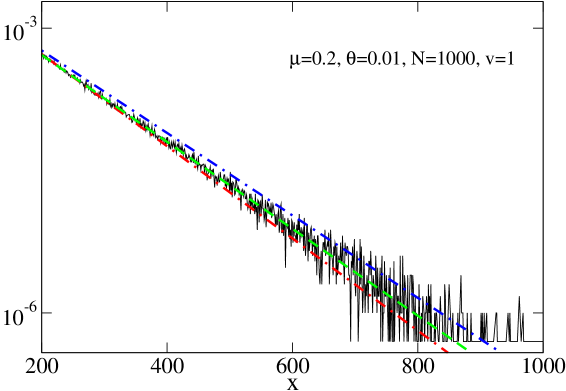
Figure 1: Monte Carlo profile involving $N=10^{3}$ cells at time $t=10^{3}$ (black line), stationary upper bound (56) (blue line) and lower bound (62) (red line) profiles with parameters: the anomalous exponent $\mu=0.2,$ the death rate $\theta=0.01,$ the time unit $\tau_{0}=1$ and the cell velocity $v=1.$

5 Conclusion

We have been motivated by experiments showing non-Markovian subballistic superdiffusive dynamics of cells [6, 7, 8, 9, 10]. The main challenge was to implement the random death process into a non-Markovian transport processes governed by the anomalously persistent random walks. We presented a Markovian model of cell motility that accounts for the effects of a random death process and the dependence of switching rates on the residence time variable $\tau$. Our purpose was to extend the the standard model for the velocity-jump random walk with reactions for the anomalous case of Lévy walks involving intermediate subballistic superdiffusive motion. We derived non-Markovian master equations for the cell densities with the generalized switching terms involving the tempered fractional material derivatives. The cell degradation rate plays the role of a tempering parameter. In the long-time limit we derived stationary master equations in terms of exponentially truncated fractional derivatives in which the rate of death tempers a Lévy jump distribution. We find the upper and  lower bounds for the stationary profiles corresponding to the ballistic transport and diffusion with the death rate dependent diffusion coefficient. Monte Carlo simulations confirm these bounds.

The main advantage of our model is that it can be extended to the case of nonlinear death rate $\theta(\rho)$ that depends on the total density of cells $\rho$. An important application of the results of this paper may be the problem of wave propagation in reaction–transport systems involving random walks with finite jump speed and memory effects [50, 51]. It would also be interesting to explore the long-memory effects in the context of persistent random walks with random velocities [13]. It is also of great interest to analyze the nonlinear tempering phenomenon leading to the nonlinear diffusion [52].

6 Acknowledgment.

This work was funded by EPSRC grant EP/J019526/1. The authors wish to thank Nickolay Korabel and Steven Falconer for very useful discussions.

7 Appendix 1

The purposes of this Appendix are (A) to express the switching functions $i_{+}(x,t)$ and $i_{-}(x,t)$ in terms of $\rho_{+}(x,t)$ and $\rho_{-}(x,t);$ (B) to derive the master equations for the unstructured density $\rho_{+}(x,t),$ $\rho_{-}(x,t)$ (14) and (15); (C) to find the Fourier-Laplace transform of the total density $\rho(x,t)=\rho_{+}(x,t)+\rho_{-}(x,t).$

(A) Substitution of (13) into (4) and (12) together with the initial condition (3) gives

$$i_{+}(x,t)=\int_{0}^{t^{-}}i_{-}(x-v\tau,t-\tau)\psi(\tau)e^{-\theta\tau}d\tau+\rho_{+}^{0}(x-vt)\psi(t)e^{-\theta t},$$

$$i_{-}(x,t)=\int_{0}^{t^{-}}i_{+}(x+v\tau,t-\tau)\psi(\tau)e^{-\theta\tau}d\tau+\rho_{-}^{0}(x+vt)\psi(t)e^{-\theta t}$$ (63)

and

$$\rho_{+}(x,t)=\int_{0}^{t^{-}}i_{-}(x-v\tau,t-\tau)\Psi\left(\tau\right)e^{-\theta\tau}d\tau+\rho_{+}^{0}(x-v\tau)\Psi\left(t\right)e^{-\theta t},$$

$$\rho_{-}(x,t)=\int_{0}^{t^{-}}i_{+}(x+v\tau,t-\tau)\Psi\left(\tau\right)e^{-\theta\tau}d\tau+\rho_{-}^{0}(x+v\tau)\Psi\left(t\right)e^{-\theta t}.$$ (64)

Applying the Fourier-Laplace transform together with shift theorem to above equations, we find expressions for $i_{+}(x,t)$ and $i_{-}(x,t)$ in terms of $\rho_{+}(x,t)$ and $\rho_{-}(x,t).$ By using (19) and (20), we obtain from (63) and (64)

$$\tilde{\imath}_{\pm}(k,s)=\left[\tilde{\imath}_{\mp}(k,s)+\rho_{\pm}^{0}(k)\right]\hat{\psi}(s\mp ikv+\theta),$$ (65)

$$\tilde{\rho}_{\pm}(k,s)=\left[\tilde{\imath}_{\mp}(k,s)+\rho_{\pm}^{0}(k)\right]\hat{\Psi}(s\mp ikv+\theta).$$ (66)

Therefore

$$\tilde{\imath}_{\pm}(k,s)=\frac{\hat{\psi}(s\mp ikv+\theta)}{\hat{\Psi}(s\mp ikv+\theta)}\tilde{\rho}_{\pm}(k,s).$$

The inverse Fourier-Laplace transform gives (16).

(B) It is convenient to introduce the following notations

$$\hat{\Psi}_{\theta}^{\pm}=\hat{\Psi}(s\pm ikv+\theta),\ \hat{\psi}_{\theta}^{\pm}=\hat{\psi}(s\pm ikv+\theta),$$

then solving (65) and (66) for $\tilde{\rho}_{+}$ and $\tilde{\rho}_{-}$ we find

$$\tilde{\rho}_{+}(k,s)=\left[\frac{\hat{\psi}_{\theta}^{+}\tilde{\rho}_{-}(k,s)}{\hat{\Psi}_{\theta}^{+}}+\rho_{+}^{0}(k)\right]\hat{\Psi}_{\theta}^{-},$$ (67)

$$\tilde{\rho}_{-}(k,s)=\left[\frac{\hat{\psi}_{\theta}^{-}\tilde{\rho}_{+}(k,s)}{\hat{\Psi}_{\theta}^{-}}+\rho_{-}^{0}(k)\right]\hat{\Psi}_{\theta}^{+}.$$ (68)

These two equations can be rewritten as

$$\frac{\tilde{\rho}_{+}(k,s)}{\hat{\Psi}_{\theta}^{-}}-\rho_{+}^{0}(k)=\frac{\hat{\psi}_{\theta}^{+}\tilde{\rho}_{-}(k,s)}{\hat{\Psi}_{\theta}^{+}},$$

$$\frac{\tilde{\rho}_{-}(k,s)}{\hat{\Psi}_{\theta}^{+}}-\rho_{-}^{0}(k)=\frac{\hat{\psi}_{\theta}^{-}\tilde{\rho}_{+}(k,s)}{\hat{\Psi}_{\theta}^{-}}.$$

Then

$$\frac{\tilde{\rho}_{+}(k,s)}{\hat{\Psi}_{\theta}^{-}}\left[1-\hat{\psi}_{\theta}^{-}\right]-\rho_{+}^{0}(k)=-\frac{\hat{\psi}_{\theta}^{-}\tilde{\rho}_{+}(k,s)}{\hat{\Psi}_{\theta}^{-}}+\frac{\hat{\psi}_{\theta}^{+}\tilde{\rho}_{-}(k,s)}{\hat{\Psi}_{\theta}^{+}},$$

$$\frac{\tilde{\rho}_{-}(k,s)}{\hat{\Psi}_{\theta}^{+}}\left[1-\hat{\psi}_{\theta}^{+}\right]-\rho_{-}^{0}(k)=-\frac{\hat{\psi}_{\theta}^{+}\tilde{\rho}_{-}(k,s)}{\hat{\Psi}_{\theta}^{+}}+\frac{\hat{\psi}_{\theta}^{-}\tilde{\rho}_{+}(k,s)}{\hat{\Psi}_{\theta}^{-}}.$$

Since $\left[1-\hat{\psi}_{\theta}^{\pm}\right]/\hat{\Psi}_{\theta}^{\pm}=s\mp ikv+\theta$, we obtain

$$\left(s+ikv+\theta\right)\tilde{\rho}_{+}(k,s)-\rho_{+}^{0}(k)=-\frac{\hat{\psi}_{\theta}^{-}\tilde{\rho}_{+}(k,s)}{\hat{\Psi}_{\theta}^{-}}+\frac{\hat{\psi}_{\theta}^{+}\tilde{\rho}_{-}(k,s)}{\hat{\Psi}_{\theta}^{+}},$$

$$\left(s-ikv+\theta\right)\tilde{\rho}_{-}(k,s)-\rho_{-}^{0}(k)=-\frac{\hat{\psi}_{\theta}^{+}\tilde{\rho}_{-}(k,s)}{\hat{\Psi}_{\theta}^{+}}+\frac{\hat{\psi}_{\theta}^{-}\tilde{\rho}_{+}(k,s)}{\hat{\Psi}_{\theta}^{-}}.$$

The left-hand sides are the Fourier-Laplace transforms of $\partial\rho_{\pm}/\partial t\pm\partial\rho_{\pm}/\partial x-\theta\rho_{+},$ therefore, these two equations are the the Fourier-Laplace transforms of the master equations (14) and (15).

(C) From (67) and (68) we find explicit expressions for $\tilde{\rho}_{+}(k,s)$ and $\tilde{\rho}_{-}(k,s):$

$$\tilde{\rho}_{+}(k,s)=\frac{\rho_{+}^{0}(k)\hat{\Psi}_{\theta}^{-}+\rho_{-}^{0}(k)\hat{\Psi}_{\theta}^{-}\hat{\psi}_{\theta}^{+}}{1-\hat{\psi}_{\theta}^{+}\hat{\psi}_{\theta}^{-}},$$ (69)

$$\tilde{\rho}_{-}(k,s)=\frac{\rho_{-}^{0}(k)\hat{\Psi}_{\theta}^{+}+\rho_{+}^{0}(k)\hat{\Psi}_{\theta}^{+}\hat{\psi}_{\theta}^{-}}{1-\hat{\psi}_{\theta}^{+}\hat{\psi}_{\theta}^{-}}.$$ (70)

The Fourier-Laplace transform of the total density $\rho(x,t)=\rho_{+}(x,t)+\rho_{-}(x,t)$ is $\tilde{\rho}_{+}(k,s)+\tilde{\rho}_{-}(k,s).$ Using (69) and (70), we obtain (22).

8 Appendix 2: anomalous switching $\mu<1$.

In this Appendix we consider the case when the death rate $\theta=0$ and all cells start at $t=0$ to move on the right with the velocity $v$ from the point $x=0:$

$$\rho_{+}^{0}(x)=\delta\left(x\right),\quad\rho_{-}^{0}(x)=0.$$

Then $\rho_{+}^{0}(k)=1$ and $\rho_{-}^{0}(k)=0.$ It follows from (22) that

$$\tilde{\rho}(k,s)=\frac{\hat{\Psi}(s-ikv)+\hat{\Psi}(s+ikv)\hat{\psi}(s-ikv)}{1-\hat{\psi}(s+ikv)\hat{\psi}(s-ikv)}.$$

By using this formula, we can find the Laplace transforms of the first moment $\mathbb{E}\left\{x(t)\right\}$ as

$$\mathbb{E}\left\{x(s)\right\}=\frac{\partial\tilde{\rho}(k,s)}{\partial\left(ik\right)}|_{k=0}.$$

When $\mu<1$ the first moment $<T>=\int_{0}^{\infty}\tau\psi(\tau)\tau$ is divergent. We obtain

$$\mathbb{E}\left\{\hat{x}(s)\right\}\simeq\frac{v\Gamma(1-\mu)\tau_{0}^{\mu}}{2s^{2-\mu}}.$$

Inverse Laplace transform gives

$$\mathbb{E}\left\{x(t)\right\}\simeq\frac{v\tau_{0}^{\mu}}{2}t^{1-\mu}.$$ (71)

The same anomalous behaviour of the first moment $\mathbb{E}\left\{x(t)\right\}$ was obtained for the fractional Kramers equation [18] (see also Appendix 4).

9
Appendix 3: anomalous switching $1<\mu<2$.

In this Appendix we discuss the case when the death rate $\theta=0$ and $1<\mu<2.$ The purpose is to show that cell motility exhibits subballistic superdiffusive behaviour. We consider now the symmetrical initial conditions for which $\mathbb{E}\left\{x(t)\right\}=0$. At $t=0$ the cells start to move from the point $x=0$ as follows

$$\rho_{+}^{0}(x)=\frac{1}{2}\delta\left(x\right),\quad\rho_{-}^{0}(x)=\frac{1}{2}\delta\left(x\right).$$

Their Fourier transforms are equal: $\rho_{+}^{0}(k)=\rho_{-}^{0}(k)=1/2.$ Let us find the mean square displacement $\mathbb{E}\left\{x^{2}(t)\right\}$. The formula for $\tilde{\rho}(k,s)$ is

$$\tilde{\rho}(k,s)=\frac{\left(1+\hat{\psi}(s+ikv)\right)\hat{\Psi}(s-ikv)+\left(1+\hat{\psi}(s-ikv)\right)\hat{\Psi}(s+ikv)}{2\left[1-\hat{\psi}(s+ikv)\hat{\psi}(s-ikv)\right]}$$ (72)

which was firstly obtained by CTRW formalism (see Eq. (9) together with (11) in [14]). One can find the Laplace transform of the second moment $\mathbb{E}\left\{x^{2}(t)\right\}$ using $\tilde{\rho}(k,s)$ from (72) as

$$\mathbb{E}\left\{x^{2}(s)\right\}=\frac{\partial^{2}\tilde{\rho}(k,s)}{\partial\left(ik\right)^{2}}_{|k=0}=\frac{2v^{2}}{s^{3}}+\frac{4v^{2}\hat{\psi}^{\prime}(s)}{s^{2}\left(1-\hat{\psi}^{2}(s)\right)}.$$ (73)

We consider the switching rate (8) with $1<\mu<2$ when the first moment $<T>=\int_{0}^{\infty}\tau\psi(\tau)\tau$ is finite, while the variance is divergent. The small $s$ expansion of $\hat{\psi}\left(s\right)$ can be written as

$$\hat{\psi}\left(s\right)\simeq 1-<T>s+A<T>s^{\mu}.$$ (74)

Substitution of (74) into (73) gives

$$\mathbb{E}\left\{x^{2}(s)\right\}\simeq\frac{2A\left(\mu-1\right)v^{2}}{s^{4-\mu}}.$$

This formula allows us to find the mean squared displacement $\mathbb{E}\left\{x^{2}(t)\right\}$ which exhibits subballistic superdiffusive behaviour [14]

$$\mathbb{E}\left\{x^{2}(t)\right\}\simeq\frac{2A\left(\mu-1\right)v^{2}}{\Gamma(4-\mu)}t^{3-\mu}.$$

as $t\rightarrow\infty.$

10 Appendix 4: velocity autocovariance and mean cell position

The purpose of this Appendix is to find the mean cell position and to show that the cell velocity has a long memory for $\mu<1$. Let the cell’s velocity at the initial time be positive, $v(0)=v,$ then the velocity $v(t)$ and the position $x(t)$ of cell can be defined as

$$v(t)=(-1)^{N(t)}v,$$ (75)

$$x(t)=v\int_{0}^{t}(-1)^{N(u)}du,$$ (76)

where $N(t)$ is the random number of switching up to time $t$ [39]. Autocovariance $C_{v}(t)=\mathbb{E}\left(v(t)v(0)\right)$ and the mean cell position $\mathbb{E}\left(x(t)\right)$ can be found as

$$C_{v}(t)=v^{2}\mathbb{E}\left\{(-1)^{N(t)}\right\}=v^{2}\sum_{n=0}^{\infty}(-1)^{n}P(n,t),$$ (77)

$$\mathbb{E}\left\{x(t)\right\}=v\mathbb{E}\left\{\int_{0}^{t}(-1)^{N(u)}du\right\}=v\sum_{n=0}^{\infty}(-1)^{n}\int_{0}^{t}P(n,u)du,$$ (78)

where $P(n,t)=\Pr(N(t)=n).$ We should note that in the anomalous case $\mu<1,$ the random velocity $v(t)$ is non-stationary process. The Laplace transform of $C_{v}(t)$ and $\mathbb{E}\left(x(t)\right)$ are

$$\hat{C}_{v}(s)=v^{2}\sum_{n=0}^{\infty}(-1)^{n}\hat{P}(n,s),$$ (79)

$$\mathbb{E}\left\{\hat{x}(s)\right\}=v\sum_{n=0}^{\infty}(-1)^{n}\frac{\hat{P}(n,s)}{s},$$ (80)

where the Laplace transform of $P(n,t)$ is given by [37]

$$\hat{P}(n,s)=\frac{\tilde{\psi}^{n}(s)(1-\tilde{\psi}(s))}{s}.$$ (81)

The substitution of (81) into (79) gives

$$\hat{C}_{v}(s)=\frac{v^{2}(1-\tilde{\psi}(s)}{s}\sum_{n=0}^{\infty}(-1)^{n}\tilde{\psi}^{n}(s)=\frac{v^{2}(1-\tilde{\psi}(s)}{s\left(1+\tilde{\psi}(s)\right)}.$$

When the mean waiting time $\langle T\rangle=\int_{0}^{\infty}\tau\psi(\tau)d\tau$ is infinite, the Laplace transform $\tilde{\psi}(s)$ can be approximated for small $s$ by Eq. (28). In this case we obtain

$$\hat{C}_{v}(s)\simeq\frac{v^{2}\Gamma(1-\mu)\tau_{0}^{\mu}}{2s^{1-\mu}},$$

$$\mathbb{E}\left\{\hat{x}(s)\right\}\simeq\frac{v\Gamma(1-\mu)\tau_{0}^{\mu}}{2s^{2-\mu}}.$$

Inverse Laplace transform gives the large time asymptotics for $0<\mu<1:$

$$C_{v}(t)\simeq\frac{v^{2}\tau_{0}^{\mu}}{2t^{\mu}},\;\;$$

$$\mathbb{E}\left\{x(t)\right\}\simeq\frac{v\tau_{0}^{\mu}}{2}t^{1-\mu}.$$

References

- [1] A. J. Ridley, M. A. Schwartz, K. Burridge, R. A. Firtel, M. H. Ginsberg, G. Borisy, J. T. Parsons, A. R. Horwitz. Cell migration: integrating signals from front to back. Science 302 (2003), 1704-1709.
- [2] R. Erban, H. Othmer. From individual to collective behaviour in bacterial chemotaxis. SIAM J. Appl. Math. 65 (2004), No. 2, 361–391.
- [3] W. Alt. Biased random walk models for chemotaxis and related diffusion approximations, J. Math. Biology 9 (1980), 147-177.
- [4] H. G. Othmer, A. Stevens. Aggregation, blowup, and collapse: The ABC’s of taxis in reinforced random walks. SIAM J. Appl. Math., 57 (1997), 1044-1081.
- [5] R. E. Baker, Ch. A. Yates, R. Erban. From microscopic to macroscopic descriptions of cell migration on growing domains. Bull. Math. Biology 72 (2010), 719–762.
- [6] A. Upadhyayaa, J-P Rieub, J. A. Glaziera, Y. Sawadac. Anomalous diffusion and non-Gaussian velocity distribution of Hydra cells in cellular aggregates. Physica A 293 (2001) 549–558.
- [7] P. Dieterich, R. Klages, R. Preuss, A. Schwab. Anomalous dynamics of cell migration. PNAS 105 (2008), 459-463.
- [8] H. Takagi, M. J. Sato, T. Yanagida, M. Ueda. Functional analysis of spontaneous cell movement under different physiological conditions. PLoS One 3 (2008), e2648.
- [9] C. T. Mierke, B. Frey, M. Fellner, M. Herrmann and B. Fabry. Integrin facilitates cancer cell invasion through enhanced contractile forces, J. Cell Sci. 124 (2011), 369-383.
- [10] C. T. Mierke, The integrin alphav beta increases cellular stiffness and cytoskeletal remodeling dynamics to facilitate cancer cell invasion, New Journal of Physics 15 (2013), 015003 (23pp).
- [11] J. Klafter, A. Blumen, and M. F. Shlesinger, Stochastic pathway to anomalous diffusion, Phys. Rev. A 35 (1987), 3081-3085.
- [12] R. Metzler, J. Klafter. The random walk’s guide to anomalous diffusion: a fractional dynamics approach. Phys. Rep. 339 (2000), 1-77.
- [13] V. Zaburdaev, S. Denisov, and J. Klafter, Lévy walks, arxiv.org/1410.5100 (2014).
- [14] J. Masoliver, K. Lindenberg, and G. H. Weiss, A continuous-time generalization of the persistent random walk, Physica A 157 (1989), 891–898.
- [15] R. Ferrari, A. J. Manfroi, and W. R. Young, Strongly and weakly self-similar diffusion, Physica D 154 (2001), 111 - 137.
- [16] ] I. M. Sokolov and R. Metzler, Towards deterministic equations for Lévy walks: The fractional material derivative. Phys. Rev. E 67 (2003), 010101 (R).
- [17] B. J. West, P. Grigolini, R. Metzler, Th. F. Nonnenmacher, Fractional diffusion and Lévy stable processes. Phys. Rev. E, 55 (1997), 99-106.
- [18] E. Barkai and R. J. Silby, Fractional Kramers equation, J. Phys. Chem. B 104 (2000), 3866-3874.
- [19] S. Fedotov, G. N. Milstein, and M. V. Tretyakov Superdiffusion of a random walk driven by ergodic Markov process with switching. J. Phys. A: Math. Theor. 40 (2007) 5769-5782 .
- [20] V. Mendez, S. Fedotov, and W. Horsthemke, Reaction-Transport Systems (Springer, Berlin, 2010).
- [21] K. P. Hadeler, in Stochastic and Spatial Structures of Dynamical Systems, edited by S. J. van Strien and S. M. Verduyn Lunel (North-Holland, Amsterdam, 1996), 133–161.
- [22] W. Horsthemke. External Noise and Front Propagation in Reaction-Transport Systems with Inertia: The Mean Speed of Fisher Waves, Fluct. Noise Lett. 2 (2002) R109 - R124.
- [23] T. Hillen. Existence Theory for Correlated Random Walks on Bounded Domains, Canad. Appl. Math. Quart. 18 (2010), 1-40.
- [24] E. Bouin, V. Calvez, G. Nadin. Hyperbolic travelling waves driven by growth, Math. Models Methods, Appl. Sci. 24 (2014), 1165–1195.
- [25] V. Mendez, D. Campos, and W. Horsthemke. Growth and dispersal with Inertia: Hyperbolic reaction-transport systems, Phys. Rev. E (2014), 042114.
- [26] A. Iomin. A toy model of fractal glioma development under RF electric field treatment. Eur. Phys. J. E 35 (2012), 42.
- [27] E. Abad, S. B. Yuste, K. Lindenberg. Reaction-subdiffusion and reaction-superdiffusion equations for evanescent particles performing continuous-time random walks. Phys. Rev. E 81 (2010), 031115.
- [28] S. Fedotov, A. O. Ivanov and A. Y. Zubarev Non-homogeneous Random Walks, Subdiffusive Migration of Cells and Anomalous Chemotaxis, Mathematical Modelling of Natural Phenomena 8 (2013) 28-43.
- [29] C. N. Angstmann, I. C. Donnelly, B. I. Henry, Continuous time random walks with reactions forcing and trapping, Mathematical Modelling of Natural Phenomena 8 (2013), 17-27.
- [30] S. Fedotov and S. Falconer Random death process for the regularization of subdiffusive fractional equations. Phys. Rev. E 87 (2013), 052139.
- [31] D. R. Cox, H. D. Miller. The Theory of Stochastic Processes (Methuen, London, 1965).
- [32] E. Scalas, R. Gorenflo, F. Mainardi, and M. Raberto, Revisiting the derivation of the fractional diffusion equation. Fractals 11 (2003), 281-289.
- [33] S. Fedotov and A. Iomin, Probabilistic approach to a proliferation and migration dichotomy in tumor cell invasion. Phys. Rev. E 77 (2008), 031911 .
- [34] S. Fedotov and V. Mendez, Non-Markovian model for transport and reactions of particles in spiny dendrites. Phys. Rev. Lett. 101 (2008), 218102 .
- [35] S. Fedotov, H. Al-Shamsi, A. Ivanov and A. Zubarev Anomalous transport and nonlinear reactions in spiny dendrites. Phys. Rev. E 82 (2010), 041103.
- [36] V. M. Kenkre, E. W. Montroll, M. F. Shlesinger: Generalized Master Equations for Continuous-Time Random Walks. J. Stat. Phys. 9 (1973), 45-50.
- [37] W. Feller. An Introduction to Probability Theory and Its Applications. (Wiley, New York, 1966).
- [38] S. Goldstein, On diffusion by discontinuous movements and on the telegraph equation. Q. J. Mech. Appl. Math. 4 (1951), 129-156.
- [39] M. Kac. A stochastic model related to the telegrapher’s equation., Rocky Mountain J. Math. 4 (1974), 497-509.
- [40] A. Di Crescenzo, On random motions with velocities alternating at Erlang-distributed random times. Advances in Applied Probability, 33 (2001) 690–701.
- [41] A. Di Crescenzo, B. Martinucci, Random Motion with Gamma-Distributed Alternating Velocities in Biological Modeling, Computer Aided Systems Theory – EUROCAST 2007, Lecture Notes in Computer Science Volume 4739, 2007, 163-170.
- [42] M. M. Meerschaert, D. A. Benson, H. P. Scheffler, and P. Becker-Kern. Governing equations and solutions of anomalous random walk limits, Physical Review E, 66 (2002), 102R-105R.
- [43] P. Becker-Kern, M. M. Meerschaert and H. P. Scheffler. Limit theorems for coupled continuous time random walks. Ann. Probab. 32 (2004), 730–756.
- [44] B. Baeumer, M. M. Meerschaert, J. Mortensen. Space-time fractional derivative operators. Proceedings of the American Mathematical Society 133 (2005), 2273–2282.
- [45] S. G. Samko, A. A. Kilbas, and O. I. Marichev. Fractional Integrals and Derivatives. (Gordon and Breach, Amsterdam, 1993).
- [46] A. Cartea and D. del-Castillo-Negrete. Fluid limit of the continuous-time random walk with general Lévy jump distribution functions, Phys. Rev. E 76, (2007) 041105 .
- [47] B. Baeumer, M. M. Meerschaert. Tempered stable Lévy motion and transient super-diffusion, J. Comput. Appl. Math 233 (2010) 243–248.
- [48] F. Sabzikara, M. M. Meerschaert, and J. Chen. Tempered fractional calculus, J. Comp. Physics (2014, in press).
- [49] J. Beran, Statistics for long-memory processes. (Chapman and Hall, New York, 1994).
- [50] V. Méndez, D Campos, S. Fedotov. Front propagation in reaction-dispersal models with finite jump speed, Phys. Rev. E 70 (2004), 036121.
- [51] A Yadav, S. Fedotov, V. Méndez, W. Horsthemke. Propagating fronts in reaction–transport systems with memory, Physics Letters A 371 (5), 374-378.
- [52] S. Fedotov and S. Falconer. Nonlinear degradation-enhanced transport of morphogens performing subdiffusion. Phys. Rev. E 89 (2014), 012107.